The sensitivity of Fama-French factors to economic uncertainty

HAL Id: hal-01015702https://hal.archives-ouvertes.fr/hal-01015702

Preprint submitted on 26 Jun 2014

HAL is a multi-disciplinary open accessarchive for the deposit and dissemination of sci-entific research documents, whether they are pub-lished or not. The documents may come fromteaching and research institutions in France orabroad, or from public or private research centers.

L’archive ouverte pluridisciplinaire HAL, estdestinée au dépôt et à la diffusion de documentsscientifiques de niveau recherche, publiés ou non,émanant des établissements d’enseignement et derecherche français ou étrangers, des laboratoirespublics ou privés.

The sensitivity of Fama-French factors to economicuncertainty

Amélie Charles, Olivier Darné, Zakaria Moussa

To cite this version:Amélie Charles, Olivier Darné, Zakaria Moussa. The sensitivity of Fama-French factors to economicuncertainty. 2014. �hal-01015702�

https://hal.archives-ouvertes.fr/hal-01015702

https://hal.archives-ouvertes.fr

EA 4272

The sensitivity of Fama-French factors to economic uncertainty

Amélie Charles* Olivier Darné**

Zakaria Moussa**

2014/20

(*) School of Management - Audencia Nantes (**) LEMNA - Université de Nantes

Laboratoire d’Economie et de Management Nantes-Atlantique

Université de Nantes Chemin de la Censive du Tertre – BP 52231

44322 Nantes cedex 3 – France

www.univ-nantes.fr/iemn-iae/recherche

Tél. +33 (0)2 40 14 17 17 – Fax +33 (0)2 40 14 17 49

Do

cum

ent

de

Tra

vail

Wo

rkin

g P

aper

The sensitivity of Fama-French factors

to economic uncertainty∗

Amélie CHARLES†

Audencia Nantes, School of Management

Olivier DARNÉ‡

LEMNA, University of Nantes

Zakaria MOUSSA§

LEMNA, University of Nantes

Preliminary version - Comments welcome

∗We thank Nicholas Bloom, Rüdiger Bachmann, Kenneth French, Sydney Ludvington, and Lubos Pastor for providing their

data. Olivier Darné and Zakaria Moussa gratefully acknowledge financial support from the Chaire Finance of the University

of Nantes Research Foundation.†Audencia Nantes, School of Management, 8 route de la Jonelière, 44312 Nantes Cedex 3. Email: [email protected].‡Corresponding author: LEMNA, University of Nantes, IEMN–IAE, Chemin de la Censive du Tertre, BP 52231, 44322

Nantes, France. Email: [email protected].§LEMNA, University of Nantes, IEMN–IAE, Chemin de la Censive du Tertre, BP 52231, 44322 Nantes, France. Email:

[email protected].

Abstract

This paper analyzes the sensitivity of the three Fama-French factors in relation to the US eco-

nomic uncertainty, by using three proxies of uncertainty measures in macroeconomics, financial

markets or economic policy from January 1985 to December 2011. We examine the extent, speed

and duration of response of the three (market, size and value) risk premia to movements in the

US uncertainties under low and high volatility regimes through the Markov-regime switching VAR

model. We find clearly two (high and low) volatility regimes, where each regime is highly persistent.

The high volatility regime is the prevailing regime between periods of 2000 to 2003, and 2008 to the

end of 2012. We show a negative effect of changes in financial and economic policy uncertainties on

value risk premia during the high volatility regime. This finding imply that investors move to growth

stocks from value stocks in high volatility regime when volatility is expected to increase. The latter

suggests that value firms can be more risky than growth firms during high volatility periods. We

also propose an aggregate measure of economic uncertainty by using Principal Component Analysis

based on the three uncertainty proxies. The results on value risk premia are confirmed. We find a

negative relationship between the market risk premium and the change in the economic uncertainty

index in high volatility regime. Finally, by adding a liquidity risk factor we find a positive effect of

financial uncertainty on liquidity factor during the high volatility regime, suggesting that investors

preferring liquidity stocks when market uncertainty increases.

Keywords: Fama-French factors; Economic uncertainty; Markov-switching model.

JEL Classification: G10; G11; C32.

1 Introduction

The Capital Asset Pricing Model (CAPM) of Sharpe (1964), Lintner (1965), and Mossin (1966) remains

a benchmark asset pricing model for both financial economists and investment practitioners, which

relates required or expected returns to systematic risk (or market beta) and not related to other variables.1

However, some firm-specific characteristics besides the market beta have been documented to have

significant explanatory power for average returns, for example, firm size (e.g., Banz, 1981; Reinganum,

1981, 1982), and book-to-market equity ratio (B/M) (e.g., De Bondt and Thaler, 1985; Fama and French,

1992). Motivated by the growing empirical evidence on these CAPM anomalies, Fama and French

(1993) propose a three-factor model (FF) that adds two factors to the market risk premium, size and

value (premia) factors.

It is considered that value (growth) stocks are riskier than growth (value) stocks in bad (good) times

(e.g., Jagannathan and Wang, 1996; Lettau and Ludvigson, 2001b; Petkova and Zhang, 2005; Zhang,

2005; Chen et al., 2008), suggesting that investors tend to switch from riskier assets to safer ones in bad

times. Further, since small firms are relatively more sensitive to economic downturns than large firms

(e.g., Gertler and Gilchrist, 1994; Fort et al., 2013), investors tend to move out of small stocks in bad

times.

It is also well-known that uncertainty about the future has real implications on economic agents’ be-

havior (e.g., Dixit, 1989; Bernanke, 1983; Bloom et al., 2007; Bloom, 2009). Growing literature provide

evidence that economic uncertainty affect financial markets, especially firm fundamentals, such as cash

flows, risk-adjusted discount factors, and investment opportunities (e.g., Bloom, 2009; Bloom, Bond,

and Van Reenen, 2007), equity portfolios and individual stocks (e.g., Anderson et al., 2009; Bekaert et

al., 2009; Bali and Zhou, 2013), and volatility (e.g., Veronesi, 1999; Bansal and Yaron, 2004; Bloom,

2009). Recently, Brogaard and Detzel (2013) show that uncertainty related specifically to the economic

policy of governments may impact financial markets. Economic uncertainty is difficult to quantify since

it is intrinsically unobservable concept, and there are different sources of uncertainty, but it is possible

to observe uncertainty indirectly using a number of proxy indicators (Bloom, 2013; Bloom et al., 2013).

This paper analyzes the sensitivity of three Fama-French factors (1993) in relation to the US

economic uncertainty, by using three proxies of uncertainty measures in macroeconomics, financial

markets or economic policy.2 We use the index of economic policy uncertainty proposed by Baker,

1See Shih et al. (2014) for a survey on the evolution of CAPM during the last four decades.2Knight (1921) established a distinction between risk and true uncertainty. Risk refers to the possibility of a future outcome

Bloom and Davis (2013), the CBOE volatility index as proxy of financial market uncertainty, and the

macro uncertainty factor developed by Jurado et al. (2013). Specifically, we investigate whether the

uncertainty measures have a direct and systematic effect on equity returns by increasing or decreasing the

returns of the systematically priced factors included in the Fama and French (1993) model. In addition

to specific measures of uncertainty, we use a statistical approach to develop an aggregate measure of

economic uncertainty. To sufficiently capture the common variation among the correlated factors of

economic policy, financial and macroeconomic uncertainty, we apply the principal component analysis

that uses orthogonal transformation to convert a set of highly correlated indicators into a set of linearly

uncorrelated variables called principal components. We then examine the sensitivity of three Fama-

French factors to this economic uncertainty index.

In particular, we examine the extent, speed and duration of response of the three (market, size and value)

risk premia to movements in the US uncertainties under low and high volatility regimes through the

application of Markov regime switching (MS) analysis (Hamilton, 1989). The MS models have become

popular in the financial literature because they can capture the instability of financial time series, such

as sudden (transitory or short-lived) or persistent changes of behavior (Ang and Timmermann, 2011).3

One of the major advantages of this approach is that it does not require prior specifications or dating

of volatility regimes. Thus, the use of the MS model allows a more robust and informative analysis on

the sensitivity of three Fama-French factors. To the knowledge of the authors, no study on the three

Fama-French factors has yet utilized the MS approach.4 In order to measure the extent of the response

of three Fama-French factors to movements in the uncertainty in economic policy, financial markets and

macroeconomics, a Markov Switching Vector Autoregressive Model (MS-VAR) is estimated. With this

model, an impulse response analysis is then conducted afterwards to determine the speed and duration

of the response. This approach allows us to analyze the effects of uncertainty in high and low volatility

periods.

The remainder of this paper is organized as follows: Section 2 briefly describes the methodology

of MS-VAR. The data are presented in Section 3. Section 4 discussed the empirical results. Finally,

Section 5 concludes.

for which the probabilities of the different possible states of the world are known. Uncertainty refers to a future outcome

that has unknown probabilities associated with the different possible states of the world. Note that some of what we call

uncertainty may indeed be risk as defined by Knight (1921). Thus, we use different proxies for economic uncertainty, which

can be different from Knightian uncertainty.3See Guidolin (2012) for a survey on applications of Markov regime switching models in empirical finance.4Durand et al. (2011) and Shamsuddin and Kim (2014) analyze the effect of the market uncertainty (using the VIX index)

on the three Fama-French factors but using a standard VAR model without regime switching.

2 Data

We consider monthly data for three Fama-French factors from January 1985 to December 2011: market

(MKT= Rm−R f )), size (Small Minus Big, SMB) and value (High Minus Low, HML) factors. The

market return (Rm) is the value-weight return of all CRSP firms incorporated in the US and listed on

the NYSE, AMEX, or NASDAQ, and the risk-free rate (R f ) is the one-month Treasury bill rate. The

SMB factor is the difference between the returns on the portfolio of small size stocks and the returns on

the portfolio of big size stocks. The HML factor is the difference between the returns on the portfolio

of high book-to-market stocks and the returns on the portfolio of low book-to-market stocks. The data

for Rm, R f , SMB and HLM come from Kenneth French’s website (see Figure 11).5 We use three

proxies of US uncertainty measures in macroeconomics, financial markets or economic policy. The US

macroeconomic uncertainty variable (UMACRO) is the macro uncertainty factor developed by Jurado et

al. (2013), based on a large number of economic time series. For the uncertainty measure in US financial

markets we employ the CBOE volatility index (VXO), also known as the “fear index” or the “fear

gauge”, based on trading of S&P 100 (OEX) options.6 The VXO reflects market uncertainty associated

with future stock price movements and might proxy risk aversion. The US economic policy uncertainty

variable that we use is the index of economic policy uncertainty (EPU) proposed by Baker, Bloom and

Davis (2013), built on three components: (i) the frequency of newspaper references to economic policy

uncertainty, (ii) the number of federal tax code provisions set to expire, and (iii) the extent of forecaster

disagreement over future inflation and government purchases.7 The span of the data is 1985:1 to 2011:12

which enables us to look at the pre- and post-crisis periods to discover the impact volatility in different

economic environments.

Figure 1 displays the three proxies of uncertainty. All uncertainty measures are higher during the 2001

economic recession and much higher during the 2008 global financial crisis. During the 1990 economic

recession the economic policy uncertainty is higher, and the financial uncertainty is moderately high.

The economic policy and financial uncertainties also present a spike around the LTCM and Russian

5The data are available on mba.tuck.dartmouth.edu/pages/faculty/ken.french/DataLibrary/.6As an alternative to the VXO index, we could have used the newer VIX index, which was introduced by the CBOE on

September 22,2003. The VIX is obtained from the European style S&P500 index option prices and incorporates information

from the volatility skew by using a broader range of strike prices than just at-the-money strike series as in the VXO. However,

the daily data on VIX starts from January 2, 1990, which does not cover our full sample period, beginning in January 1986.

The pre-1986 VXO data are calculated by Bloom (2009). See Whaley (2009) for a history of the VIX and a summary on its

calculation.7See Baker et al. (2013) for a detailed description of the EPU indexes. The data are available on

www.policyuncertainty.com/index.html.

Debt crisis of 1998. Higher uncertainty is also displayed during the October 1987 financial crisis for the

VXO, and the July 2011 debt ceiling dispute.

Table 1 provides summary statistics for the variables used in this study. The mean of the three factors

is positive, except for SMB. The risk premium factor displays the higher mean and volatility, in terms of

standard deviation. ∆VXO is the most volatile among the uncertainty measures. The three factors exhibit

negative skewness, except HML, while the three uncertainty measures display positive skewness. Excess

kurtosis is observed for all variables, showing that their empirical distributions are leptokurtic, i.e. with

substantially fatter tails (than the normal distribution). The Jarque-Bera test statistic is significant at

the 1% level of significance for all series, indicating that the variables are highly non-normal. We also

conduct the LM test of Engle (1982) for ARCH conditional heteroscedasticity.8 This test statistic is

significant for all uncertainty measures, indicating that they show strong conditional heteroscedasticity,

whereas it is non significant for the risk premium and size factors.

Table 1. Descriptive statistics

Min Max Mean S. dev. Med. Kurtosis Skewness JB test ∗ Engle LM test∗∗

MKT -23.2400 12.4600 5.7019e-01 4.6160 1.1500 5.5445 -0.8832 129.1273(1.0000e−03)

4.1559(5.2720e−01)

SMB -22.0200 8.4600 -1.3344e-01 3.2564 -0.1600 11.0036 -1.3584 961.4616(1.0000e−03)

5.5645(3.5092e−01)

HML -9.8600 13.8700 3.9133e-01 3.0884 0.2500 5.6469 0.5737 112.0088(1.0000e−03)

13.8498(1.6592e−02)

∆VXO -12.4161 32.2351 1.7851e-02 4.0333 -0.1995 18.4620 2.3841 3523.4894(1.0000e−03)

12.2971(3.0936e−02)

∆EPU/100 -0.6045 1.0377 2.3627e-03 0.1760 -0.0106 9.0484 1.1105 558.7414(1.0000e−03)

22.9068(3.5170e−04)

∆UMACRO/100 -0.4527 0.5992 1.1506e-03 0.1392 -0.0040 4.6183 0.1877 37.1408(1.0000e−03)

77.5073(2.7756e−15)

∗ In brackets, critical values for the tests. ∗∗ With 5 lags.

Table 2 displays the correlations for the whole sample. The results show a negative correlation

between uncertainty measures and risk premium factors, suggesting that an increasing in economic

uncertainty is associated with a falling market, especially from financial uncertainty (-0.56). This result

is consistent with the findings of Merton (1980), Fleming et al. (1995), Ang et al. (2006), and Durand

et al. (2011). Merton (1980) point out that the market risk premium should be positively related to

the variance of the market portfolio and that greater levels of risk should induce a larger market risk

premium. French et al. (1987) show that the expected market risk premium is positively related to

expected volatility and negatively related to unexpected changes in volatility. Ang et al. (2006) report

a negative relationship between returns and changes in expected volatility, using changes in the VXO.

8The LM test is applied on the residuals of the ARMA model, where the lag length is selected based on the Akaike

information criterion.

Figure 1. Economic policy, Financial and Macroeconomic Uncertainties.

��

��

��

��

��

��

�

��

��

��

��

��

��

��

��

� �

��

��

��

��

��

��

��

��

��

��

��

Notes: Shaded regions are NBER recession dates. The data are monthly and span the period 1985:01-2011:12.

Durand et al. (2011) show that changes in the VIX drive variations in the expected returns of the factors

included in the Fama-French three-factor model. We also find that uncertainty measures are negatively

correlated with SMB, that might also be consistent with a flight-to-quality interpretation as increasing

uncertainty may lead to investors being less willing to hold small stocks. Campbell (1993, 1996) assume

that investors want to hedge against the changes in the forecasts of future market volatilities.9 The

correlations between HML and uncertainty measures are positive and very low, as found in Durand et al.

9Bali and Engle (2010) use implied volatility from the S&P100 index options (VXO) to test whether stocks that have higher

correlation with the changes in future market volatility yield lower expected return in an ICAPM.

(2011). The results show that HML is negatively correlated to MKT (-0.27) and SMB (-0.33). Finally,

the three measures of uncertainty are positively correlated, with the highest correlation between financial

and economic policy uncertainties (0.39).

Table 2. Correlations.

MKT SMB HML ∆VXO ∆EPU/100 ∆UMACRO/100

MKT 1.00 0.19 -0.27 -0.56 -0.27 -0.18

SMB 1.00 -0.33 -0.23 -0.14 -0.10

HML 1.00 0.08 0.05 0.02

∆VXO 1.00 0.39 0.25

∆EPU/100 1.00 0.15

∆UMACRO/100 1.00

3 MS-VAR model

Markov-Switching vector autogressive (MS-VAR) model developed by Krolzig (1997) provides a

convenient framework to analysis multivariate changes in regimes. Applied to the Fama-French factors,

the Markov-switching framework offers the possibility to model high and low volatility periods as

switching regimes of the stochastic process that generates changes in the expectation of market volatility.

The model is described by equation 1. In this general specification all parameters (mean, variance

and autoregressive parameters) are allowed to switch between regimes according to hidden Markov

chain. In the terminology of Krolzig (1997) this specification is a Markov switching intercept

autoregressive heteroskedastic VAR model, MSIAH(m)-VAR(p) model, with m the number of variables

and p the lag order.

Yt =

a1+B11Yt−1+ . . . +Bp1Yt−p +A1ut i f st = 1

...

am +B1mYt−1+ . . .+BpmYt−p +Amut i f st = m

(1)

The Yt is a vector of endogenous variables which depends upon an unobserved regime variable st that

controls the state of the economy. Each regime is characterized by an intercept ai, a K dimensional

vectors of auto-regressive terms B1i, . . . ,Bpi, a matrix Ai, and fundamental disturbance ut , with ut ∼

N(0, IK). Matrix Ai is computed from the regime-dependent variance covariance matrix from the reduced

form VAR, Σi:

Σi = E(

AiUtU′t Ai′

)

= AiIAi′

In order to compute Ai, which has K2 elements and K being the number of variables, from Σi having

onlyK(K+1)

2elements, sufficient restrictions are imposed, to reach a complete identification, based on

the recursive structure using Choleski identification scheme. In this specification, the order of variables

matters. Following Durand et al. (2011), identification is achieved by assuming that Fama-French

factors (MKT, SMB and HML) do not respond contemporaneously neither to the change in the implied

volatility index (∆VIX), nor to the two measures of uncertainty (EPU and UMACRO). In other words,

the ordering of the variables in the MSIAH(4)-VAR(p) is MKT, SMB, HML and either ∆VIX, or one of

the measure of uncertainty (∆EPU or ∆UMACRO).10

According to Turner et al. (1989), Kim et al. (2004), and Abdymomunov and Morley (2011)

who found that stock market volatility follows a two-state Markov-switching process, with the market

risk premium varying across the “low” and “high” volatility regimes, 11 we assume that the number

of regimes m = 2, st .12 These two regimes conventionally corresponds to the low mean change in

volatility or stable state and the high mean change in volatility or volatile state, respectively. st = {1,2}

is assumed to follow the discrete time and discrete state stochastic process of a hidden Markov chain

and controlled by transition probabilities pi, j = Pr(st+1 = j|st = i), and ∑2j=1 pi j = 1∀i, j ∈ (1,2). The

stochastic process is defined by the transition matrix P as follows:

p =

p11 p12

p21 p22

The model is estimated using the Expectation-Maximization (EM) algorithm as suggested by

Krolzig (1997) (and in Hamilton (1994) for the univariate case), which consists of two steps whereby

10In this paper, we estimate three MSIAH(4)-VAR(p) models. In each model we include Fama-French factors and either

∆VIX or one of uncertainty measures, ∆EPU or ∆UMACRO. Of course it would be better to estimate only one model including

all our variables, but we retain this solution in order to estimate a more parsimonious models as possible. Indeed, within VAR

models, the number of variables cannot be enlarged very much, because of both estimation and identification problems. This

problem is even more present within MS-VAR models as the number of parameters to estimate grows not only with the number

of variables included in the model but also with regimes.11Schwert (1989), Schaller and van Norden (1997), Kim et al. (1998, 2001, 2004), Hess (2003) and Mayfield (2004), among

many others, have modeled monthly stock return volatility using a Markov-switching specification, with high volatility regimes

typically corresponding to periods of recession and low volatility regimes typically corresponding to periods of expansion.12We have also estimated a three-state regime models but the third regime is merely capturing a few extreme outliers in the

data, rather than persistent changes in volatility. This result is consistent with the finding of Hamilton and Susmel (1994) and

Abdymomunov and Morley (2011).

the expectation step infers the hidden Markov chain conditioned on a given set of parameters, and the

maximization step re-estimates the parameters based on the inferred unobserved Markov process. These

steps are repeated until convergence.

Our decision to use MS-VAR framework is also motivated by the possibility to derive regime-

dependent Impulse Response Functions (IRFs), which helps to determine the cyclical variation in the

responses of factors to a particular shock. For the MS-VAR models, Ehrmann et al. (2003) have

developed the regime-dependent IRFs which permit to simulate the responses of endogenous variables

to exogenous shocks. Such response functions are conditional on the prevailing regime at the time of the

shock and on the entire horizon of the response. The regime-dependent IRF13 is described by equation

2, which traces the expected path of the endogenous variables at time t + h following a one standard

deviation shock to the kth initial disturbance at time t, conditional on regime i.

θik,h =

∂EtYt+h

∂Uk,t|st = ....= st+h = i, f or h≥ 0 (2)

where θ ik,1 · · ·θ

ik,h are K dimensional response vectors of the responses of the endogenous variables to a

shock to the kth fundamental disturbance. To account for estimation uncertainty, we adopt the standard

bootstrapping method to get the related confidence bands by retaining the mean along with the relevant

percentiles of the numerical approximation of the distribution of the original estimates of the regime

vectors.14

4 Empirical results

4.1 Specific uncertainty measures

In this section, we examine the three MSIAH(4)-VARs, using one of the three proxies of US uncertainty

in financial markets, macroeconomics or economic policy, respectively. The MSIAH(4)-VAR(1)

model15 is considered according to the specification tests (see Technical Appendix). In all MSIAH(4)-

VAR(1) models, the linearity test suggests that the model is significantly non-linear and parameters

switch substantially between regimes. Moreover, for the three MSIAH(4)-VAR(1) models, each regime

is highly persistent according to the transition matrix (Table 6, Appendix A), with transition probabilities

lying between 87% and 96% month-to-month probabilities of remaining in the low and high volatility

regimes, respectively. Inferences regarding the turning points can be obtained from the smoothed

13The estimation method, identification and impulse response are detailed in Ehrmann et al. (2003).14In this analysis, we use 1000 bootstrap replicates.15The number of lags is set equal to one according to all information criteria displayed in the Technical Appendix.

probabilities of regimes (Figure 2). The timing of the change across regimes and the number of months

for which factors were under the two regimes are very similar. These results suggest that there are clearly

two different volatility regimes. Note that the first regime, corresponding to the high volatility regime,

is the prevailing regime between periods of 2000 to 2003, and 2008 to the end of 2012. These periods

correspond the bear market following the burst of the dot-com bubble and Fed’s interventions, and the

2007-2008 financial crisis and the related recession16, respectively. The second regime, corresponding

to the low volatility regime, coincides with the two bull market periods; the first was part of the dot-com

bubble and the second corresponds to the mortgage market bubble.

We also find clear spikes, commune to the three MSIAH(4)-VAR(1) models, corresponding to stock

market crash in October 1987 and the LTCM and Russian Debt crisis of 1998. A specific spike is found

from MSIAH(4)-VAR(1) using EPU in 1992 associated with the presidential election (Figure 17b).

These changes can be considered as extreme outliers, as suggested by Hamilton and Susmel (1994) who

find that “extremely large shocks, such as the October 1987 crash, arise from quite different causes and

have different consequences for subsequent volatility than do small shocks.”

We use MSIAH(4)-VAR(1) to examine the sensitivity of three risk premia (MKT, SMB and HML)

to changes in macroeconomics (∆UMACRO), financial markets (∆VXO) or economic policy (∆EPU)

uncertainties, under low and high volatility regimes. To analyze how changes in uncertainty impact the

risk premia we examine the impulse response functions (IRFs) derived from the MS-VAR, according to

the two volatility regimes. The IRFs are reported in Figure 3 along with 90% confidence band computed

with standard bootstrap. Figures 3 to 5 display how the three risk premia respond to a one standard

deviation innovation in ∆VXO, ∆EPU and ∆UMACRO, respectively. The impulse reaction period is

chosen to be 6 months. Table 3 reports the effect size estimates from the impulse response functions

with the cumulative responses. This indicates the response values of a (risk premia) variable to a standard

deviation innovation (uncertainty) shock to other over the time horizon from 0 to 6 months.

The IRFs show a positive effect of a shock to ∆VXO on SMB only during the low volatility regime

(3), implying that investors prefer larger stocks over smaller stocks in low volatility regime whereas they

move to growth stocks from value stocks in high volatility regime when volatility is expected to increase.

We also find that a negative effect of ∆VXO on HML during the high volatility regime, suggesting that

value firms can be more risky than growth firms during high volatility periods. This is consistent with

the view that value is riskier than growth in bad times when the price of risk is high (e.g., Jagannathan

16This result confirms the findings of Schwert (1989), Hamilton and Lin (1996) and Charles and Darné (2014) that volatility

of stock returns increases during (severe) recessions.

Figure 2. Estimated smoothed probabilities for MSIAH(4)-VAR(1) models

1985 1990 1995 2000 2005 2010

0.5

1.0

Smoothed prob., Regime 2 (a) MSIAH(4)-VAR(1) with VXO

1985 1990 1995 2000 2005 2010

0.5

1.0

Smoothed prob., Regime 1

(b) MSIAH(4)-VAR(1) with EPU

1985 1990 1995 2000 2005 2010

0.5

1.0


Smoothed prob., Regime 2(c) MSIAH(4)-VAR(1) with UMACRO

Note: the timeline of the figure indicates two regimes describing the sample period for different models. Regime 1,

corresponding to the high volatility regime, is represented over periods of 2000 to 2003, and 2008 to the end of 2012.

and Wang, 1996; Lettau and Ludvigson, 2001b; Petkova and Zhang, 2005; Zhang, 2005; Chen et al.,

2008). We do not find evidence of the effect of ∆VXO on MKT, whatever the volatility regime. This

result is in contrast with Durand et al. (2011) and Shamsuddin and Kim (2014) who found a negative

relationship between the market risk premium and unexpected changes in expected volatility.17

Figure 4 displays a negative effect of ∆EPU on MKT during the high volatility regime, suggesting

a negative relationship between the market risk premium and the change in the economic policy

uncertainty in high volatility regime. Contrarily to a shock to ∆VXO, the IRFs show a negative effect of

a shock to ∆EPU on SMB only during the low volatility regime. This result indicates that investors move

to large-cap firms from small-cap firms when the economic policy uncertainty increases in high volatility

regime. Finally, the IRFs displays a negative effect of ∆EPU on HML during the high volatility regime,

as for ∆VXO, with a longer horizon (5 months), and also during the low volatility regime. Note that

17Durand et al. (2011) also find that an effect of VIX is positive on HML but negligible on SMB whereas this effect

is negligible on SMB and HML for Shamsuddin and Kim (2014). These authors use the VIX index (in first-difference for

Durand et al., 2011; in level for Shamsuddin and Kim, 2014) for market uncertainty while we use the VXO index. Durand et

al. (2011) use daily data from February 1, 1993 to July 30, 2007, and Shamsuddin and Kim (2014) employ weekly data from

January 1990 to December 2011.

the impact on HML is larger from a shock to ∆VXO (-16.2%) than from a shock to ∆EPU (-4.2%) (see

Table 3). Further, the impact of EPU shock on HML is both larger and more persistent during periods

when volatility is high as opposed to periods during which volatility is lower. A 1% shock to ∆EPU

leads to 4.3% and 1.6% decline of HML during the high and low volatility regime, respectively. This is

consistent with investors preferring growth stocks over value stocks when economic policy uncertainty

increases.

The results presented in Figure 5 show that the risk premia respond to a shock to ∆UMACRO only

on MKT during the high volatility regime. This shock has very higher impact (-48.8%) than that from

a shock to ∆EPU (-6.4%), and this effect is more persistent. This finding indicates that a negative

relationship between the market risk premium and the change in the macroeconomic uncertainty in high

volatility regime. However, the change in the macroeconomic uncertainty seems to have no effect on

HML and SMB factors.

Figure 3. Response to VXO shock in MSIAH(4)-VAR(1)

3 6−0.2

0

0.2Regime 1

Rm

−R

f

3 6−0.2

0

0.2Regime 2

3 6

−0.1

0

0.1

SM

B

3 6

−0.1

0

0.1

3 6

−0.2

−0.1

0

HM

L

3 6−0.2

−0.1

0

Note: Responses of the risk premia (Rm-Rf), SMB and HML to a positive shock to VXO by one standard

deviation. The impulse reaction period is chosen to be 6 months. Solid lines show impulse responses, while

dashed lines represent confidence intervals using the 10th and 90th percentile values calculated on the basis

of 1000 bootstrap replications.

Figure 4. Response to EPU shock in MSIAH(4)-VAR(1)

3 6−0.1

−0.05

0

Regime 1R

m−

Rf

3 6−0.1

−0.05

0

Regime 2

3 6−0.05

0

0.05

SM

B

3 6−0.05

0

0.05

3 6

−0.04

−0.02

0

HM

L

3 6

−0.04

−0.02

0

Note: Responses of the risk premia (Rm-Rf), SMB and HML to a positive shock to EPU by one standard

deviation. The impulse reaction period is chosen to be 6 months. Solid lines show impulse responses, while

dashed lines represent confidence intervals using the 10th and 90th percentile values calculated on the basis

of 1000 bootstrap replications.

4.2 Economic uncertainty index

Since the three measures of uncertainty are highly positively correlated with each other (Table 2)

and they tend to move together, suggesting there is a common uncertainty component to all the

measures (Figure 1), we propose an aggregate measure of economic uncertainty (UFACTOR) by using

Principal Component Analysis (PCA).18 We use the PCA to extract the common component of the three

uncertainty proxies that capture different dimensions of the economic uncertainty: economic policy,

finance and macroeconomics. The first principal component from PCA sufficiently captures the common

variation among the three uncertainty measures.

Figure 6 presents the economic uncertainty index obtained from the first principal component of the

18Bali et al. (2014) also proposed a newly measure of macroeconomic risk associated to a quantitative indicator of economic

uncertainty, using individual measures of macroeconomic risk obtained from estimating time-varying conditional volatility of

the economic indicators based on a VAR-GARCH model. Their indicator is computed from January 1994 to March 2012.

Haddow et al. (2013) also used PCA to construct an uncertainty index based on four indicators for the UK on the 1985-2013

period.

Figure 5. Response to UMACRO shock in MSIAH(4)-VAR(1)

3 6−0.2

−0.1

0

Regime 1

Rm

−R

f

3 6−0.2

−0.1

0

Regime 2

3 6−0.1

−0.05

0

0.05

SM

B

3 6−0.1

−0.05

0

0.05

3 6−0.1

−0.05

0

0.05

HM

L

3 6−0.1

−0.05

0

0.05

Note: Responses of the risk premia (Rm-Rf), SMB and HML to a positive shock to UMACRO by one

standard deviation. The impulse reaction period is chosen to be 6 months. Solid lines show impulse

responses, while dashed lines represent confidence intervals using the 10th and 90th percentile values

calculated on the basis of 1000 bootstrap replications.

three uncertainty measures. The economic uncertainty index is generally higher during the economic

recessions, especially during the 2008 global financial crisis, and also around the October 1987 financial

crisis and the LTCM and Russian Debt crisis of 1998. This result is consistent with Bloom et al. (2012)

who find that recessions appear in periods of significantly higher economic uncertainty.

Table 4 displays the correlation between the economic uncertainty index and the three uncertainty

measures, showing that they are highly correlated. We find similar correlations between the changes

in the economic uncertainty index and the Fama-French factors, namely ∆UFACTOR is positively

correlated to MKT and SMB, and negatively to HML.

From the MS-VAR model, both regimes are highly persistent according to the transition matrix

(Table 6, Appendix A), with transition probabilities lying between 85% and 94% month-to-month

probabilities of remaining in the low and high volatility regimes, respectively. The timing of the change

across regimes and the number of months for which the economic uncertainty index is under the two

regimes are similar to our findings from specific uncertainty measures.

Table 3. Cumulative responses to shocks from period 0 to 6.

Response MKT SMB HML

Shock High Low High Low High Low

∆VXO -0.019 -0.033 0.040 0.048 -0.162 0.004

∆EPU -0.064 -0.005 0.023 -0.014 -0.043 -0.016

∆UMACRO -0.488 -0.034 -0.226 -0.018 -0.068 0.021

∆UFACTOR3 -1.685 -0.117 0.364 -0.335 -1.312 -0.823

This table reports cumulative responses to different uncertainty shocks to the three Fama-French factors.

High and Low denote high and low volatility regimes, respectively.

Figure 6. Economic Uncertainty Index based on 3 uncertainty proxies.

��

��

��

��

��

��

��

��

��



∆VXO ∆EPU/100 ∆UMACRO/100 ∆UFACTOR3 ∆UFACTOR6

∆VXO 1.00 0.39 0.25 0.82 0.82

∆EPU/100 1.00 0.15 0.83 0.71

∆UMACRO/100 1.00 0.38 0.36

∆UFACTOR3 1.00 0.93

∆UFACTOR6 1.00

MKT SMB HML ∆UFACTOR ∆UFACTOR6

MKT 1.00 0.19 -0.27 -0.50 -0.51

SMB 1.00 -0.33 -0.23 -0.26

HML 1.00 0.08 0.10

∆UFACTOR3 1.00 0.93

∆UFACTOR6 1.00

Figure 8 displays a negative effect of ∆UFACTOR on MKT during the high volatility regime,

suggesting a negative relationship between the market risk premium and the change in the economic

uncertainty index in high volatility regime. This shock to ∆UFACTOR has a higher effect on MKT than

those from ∆EPU and ∆UMACRO, with a short horizon (3 months). The IRFs displays a negative effect

of ∆UFACTOR on HML during both volatility regime, as for ∆EPU, with a longer horizon, namely 6

and 5 months, under the high and low regime, respectively, and a higher impact. This suggests that

the impact of uncertainty shock on HML is larger during periods when volatility is high as opposed to

periods during which volatility is lower. This is consistent with investors preferring growth stocks over

value stocks when global uncertainty increases.

Figure 7. Estimated smoothed probabilities for MSIAH(4)-VAR(1): UFACTOR

1985 1990 1995 2000 2005 2010

0.5

1.0



Figure 8. Response to UFACTOR shock in MSIAH(4)-VAR(1)

3 6

−2

−1

0

Regime 1

Rm

−R

f

3 6

−2

−1

0

Regime 2

3 6−1

0

1

SM

B

3 6−1

0

1

3 6−1.5

−1

−0.5

0

0.5

HM

L

3 6−1.5

−1

−0.5

0

Note: Responses of the risk premia (Rm-Rf), SMB and HML to a positive shock to UFACTOR by one




4.3 Robustness check

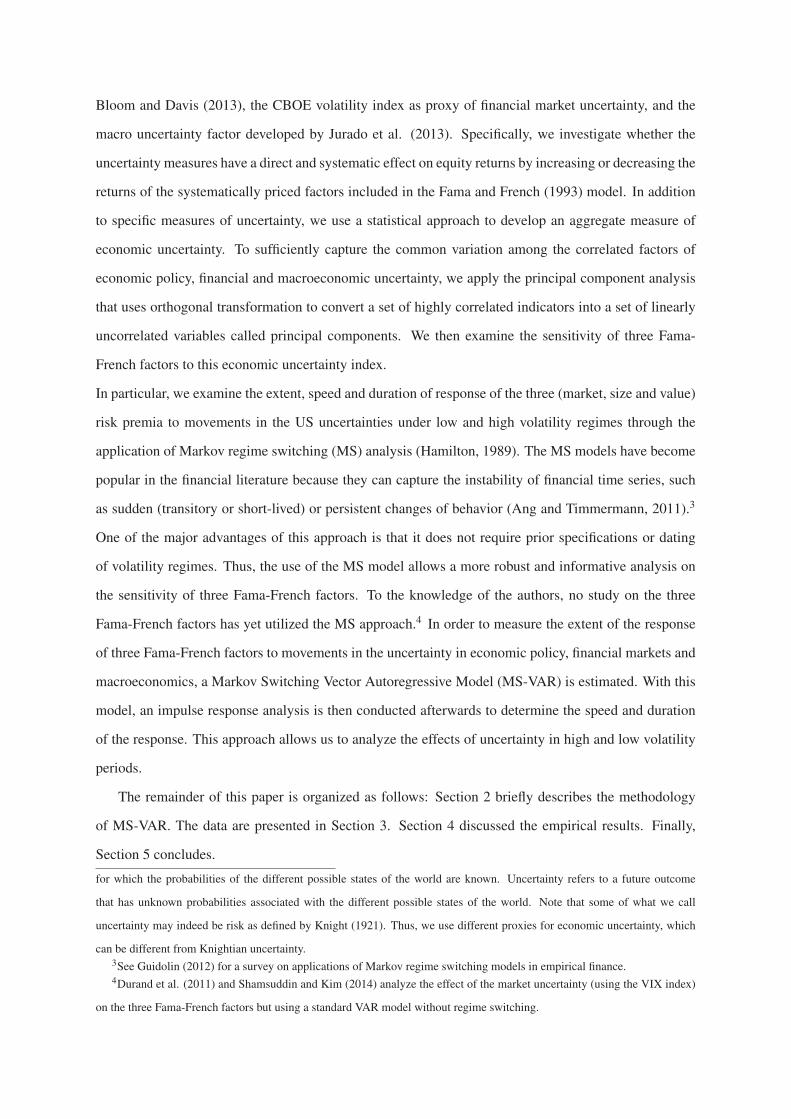
4.3.1 Momentum and Liquidity Factors

As robustness check of our results on IRFs from the MSIAH(4)-VAR(1) models with the different

measures of uncertainty, we add two others risk factors with (i) the momentum factor (Winner Minus

Loser, WML) introduced by Cahart (1997), and (ii) the aggregate liquidity factor (LIQ) proposed by

Pastor and Stambaugh (2003). Cahart (1997) proposes a four-factor model by adding this risk factor

into the Fama-French three-factor model. The phenomenon of price momentum is documented in

several studies (see, e.g., Jegadeesh and Titman, 1993; Chan et al., 1996; Fama and French, 1996;

Jegadeesh and Titman, 2001), and a number of studies show that liquidity-related risks are prices (see,

e.g., Pastor and Stambaugh, 2003; Acharya and Pedersen, 2005; Korajczyk and Sadkha, 2008; Lee,

2011). The data for WML and LIQ comes from Kenneth French’s website and from Lubos Pastor’s

website, respectively (Figure 12).19. We obtain the same results from the MSIAH(5)-VAR(1) model

than from the MSIAH(4)-VAR(1) models for (i) the both highly persistent regimes with the same timing

of the change across regimes and with slightly higher number of months for which the regime remains

in the low or high volatility regimes (Figure 14); (ii) the effects of a shock to uncertainty on risk premia

(MKT, HML and SMB) (Figure 15). These findings show the robustness of our results according to the

number of variables in the MS-VAR model.

More interesting, Figure ?? reports a short negative effect of ∆VXO on WML only during the high

volatility regime, whereas we find a positive effect of ∆EPU (Figure ??) and ∆UMACRO (Figure Figure

??) on the momentum premium, especially a highly persistent effect from a shock of macroeconomic

uncertainty.20 These results suggest that investors appear to move to proven stocks (past winners) rather

than “glamor” stocks when economic policy and macroeconomic uncertainties increase or when market

uncertainty decreases during the high volatility regime.

Further, Figure 15 displays a positive effect of ∆VXO on liquidity factor during the high volatility

regime, with a short horizon (2 months), suggesting that investors preferring liquidity stocks when

market uncertainty increases. This finding is consistent with the flight-to-liquidity phenomenon where

19The data are available on http://faculty.chicagobooth.edu/lubos.pastor/research/.20Information uncertainty has been proposed as an explanation for the abnormal returns earned via momentum strategies.

Faced with greater uncertainty, investors are increasingly unable to accurately determine the true value of an asset and are

more likely to misprice it. Zhang (2006) finds that information uncertainty exacerbates momentum, using forecast dispersion

as a measure of information uncertainty, whereas Verardo (2009) shows that investor uncertainty, based on company’s

fundamentals, is associated with less momentum. Note that Durand et al. (2011) and Kim and Shamsuddin (2014) find

that WML responds positively to a shock in VIX.

investors rebalance their portfolios toward more liquid assets. This is also consistent with Chung and

Chuwonganant (2014) who found that market uncertainty (measured by the VIX) exerts a large market-

wide impact on liquidity. We find the same result with a shock of ∆EPU (Figure 16).21

4.3.2 PCA from 6 uncertainty measures

As robustness check of our results on the aggregate measure of economic uncertainty, we consider three

others proxies of uncertainty measure to construct the economic uncertainty index in our sample. In

this respect, we use a measure of equity market uncertainty with the equity market-related economic

uncertainty (EMEU) proposed by Baker et al. (2013), a measure of financial uncertainty with the

corporate bond spreads (SPREAD), defined as the monthly spread of the 30-year Baa-rated corporate

bond yield index over the 30-year treasury bond yield, and a measure of (micro)economic (firm-specific)

uncertainty with the forecast disagreement index (FDISP) based on the forecast dispersion in the general

business situation question from the Business Outlook Survey proposed by Bachmann et al. (2013).22

These uncertainty measures are significantly correlated with the three previous measures, except for

FDISP (Table 5).


∆VXO ∆EPU/100 ∆UMACRO/100 ∆SPREAD ∆EMEU ∆FDISP ∆UFACTOR6

∆VXO 1.00 0.39 0.25 0.45 0.51 0.07 0.82

∆EPU/100 1.00 0.15 0.07 0.54 0.02 0.71

∆UMACRO/100 1.00 0.29 0.16 0.03 0.36

∆SPREAD 1.00 0.12 0.10 0.49

∆EMEU 1.00 0.02 0.77

∆FDISP 1.00 0.25

∆UFACTOR6 1.00

The economic uncertainty index is obtained by extracting the common component of the six

uncertainty proxies. Figure 13 presents the economic uncertainty index obtained from six uncertainty

measures (UFACTOR6) and also that obtained from three measures (UFACTOR3). The evolution of

both uncertainty indexes are very similar. Further, they are highly correlated (0.93, Table 4).

We find the same results from this economic uncertainty index than from the economic uncertainty

21We obtained the same results for a shock of ∆UMACRO and ∆UFACTOR on the three Fama-French factors from the

MSIAH(4)-VAR(1) and MSIAH(5)-VAR(1) models (see Technical Appendix). However, the responses to ∆UMACRO and

∆UFACTOR on the liquidity factor are non significant.22There are others proxies of uncertainty but they are not available on our sample.

Figure 9. Estimated smoothed probabilities for MSIAH(4)-VAR(1): UFACTOR6

1985 1990 1995 2000 2005 2010

0.5

1.0



index extracted from three measures for the high and low volatility regimes (Figure ??) and the responses

to an aggregate economic uncertainty shock on the three risk premia (Figure 10). These findings show

the robustness of our results on a shock of the economic uncertainty index on the MKT, SMB and HML

factors, whatever the uncertainty measures included in the index.

Figure 10. Response to UFACTOR6 shock in MSIAH(4)-VAR(1)

3 6

−2

−1

0

1

Regime 1

Rm

−R

f

3 6

−2

−1

0

1

Regime 2

3 6−1

0

1

SM

B

3 6−1

0

1

3 6−1.5

−1

−0.5

0

0.5

HM

L

3 6−1.5

−1

−0.5

0

Note: Responses of the risk premia (Rm-Rf), SMB and HML to a positive shock to UFACTOR6 by one




4.3.3 Fama-French portfolios

We study the effect of uncertainty on the 6 Fama-French benchmark portfolios formed on Size and

Book-to-Market: small value (SV), small neutral (SN), small growth (SG), big value (BV), big neutral

(BN), and big growth (BG). These portfolios, which are constructed at the end of each June, are the

intersections of 2 portfolios formed on size (market equity, ME) and 3 portfolios formed on the ratio

of book equity to market equity (BE/ME). The size breakpoint for year t is the median NYSE market

equity at the end of June of year t. BE/ME for June of year t is the book equity for the last fiscal year

end in t−1 divided by ME for December of t−1. The BE/ME breakpoints are the 30th and 70th NYSE

percentiles.

Figure 22 displays the IRFs for the 6 portfolios. The results show that a negative effect of ∆UFACTOR6

on 4 portfolios (SG, SN, SV and BV) during the high volatility regime, suggesting a negative relationship

between these portfolios and the change in the economic uncertainty index in high volatility regime.

This is consistent with the view that the small firms are more sensitive of uncertainty in bad times (high

volatility). This shock to ∆UFACTOR6 has a higher effect on SG and SV portfolios than for SN and BV

portfolios. The uncertainty shock have no effect on BG uncertainty, suggesting that big growth firms

are not affected by economic uncertainty shock, even during high volatility regime. This is consistent

with investors preferring growth stocks when economic uncertainty increases. Finally, We only find a

negative effect of ∆UFACTOR6 on BN portfolio during the low volatility regime.

5 Conclusion

This paper analyzed the sensitivity of the three Fama-French factors in relation to the US economic

uncertainty, by using three proxies of uncertainty measures in macroeconomics, financial markets or

economic policy. We examined the extent, speed and duration of response of the three risk premia to

movements in the US uncertainties under low and high volatility regimes through the MS-VAR model.

We found clearly two different volatility regimes, where each regime is highly persistent. The first

regime, corresponding to the high volatility regime, is the prevailing regime between periods of 2000 to

2003, and 2008 to the end of 2012. These periods correspond to the bear market following the burst of

the dot-com bubble and FedŠs interventions, and the 2007-08 financial crisis and the related recession,

respectively. The low volatility regime coincides with the two bull market periods; the first was part of

the dot-com bubble and the second corresponds to the mortgage market bubble.

Examining the sensitivity of three risk premia (market, size and value) to changes in macroeconomics,

financial markets or economic policy uncertainties under low and high volatility regimes, we showed a

negative effect of changes in financial and economic policy uncertainties on value risk premia during the

high volatility regime. This finding implies that investors move to growth stocks from value stocks in

high volatility regime when volatility is expected to increase. The latter suggests that value firms can be

more risky than growth firms during high volatility periods. This is consistent with the view that value

is riskier than growth in bad times when the price of risk is high (e.g., Jagannathan and Wang, 1996;

Lettau and Ludvigson, 2001b; Petkova and Zhang, 2005; Zhang, 2005; Chen et al., 2008).

Finally, we proposed an aggregate measure of economic uncertainty by using Principal Component

Analysis based on the three uncertainty proxies. The results on value risk premia are confirmed. We

also found a negative relationship between the market risk premium and the change in the economic

uncertainty index in high volatility regime.

Overall, the results of our analysis point to the sensitivity of US market and value risk premia to

economic uncertainty shock, especially during high volatility period, and warrants further research.

Figure 11. Market, size and value risk premia.

��

��

��

��

��

��

��

��

��

��

�

��

��

��

��

��

��

��

��

��

�

��

��

��

��

��

��

��

�


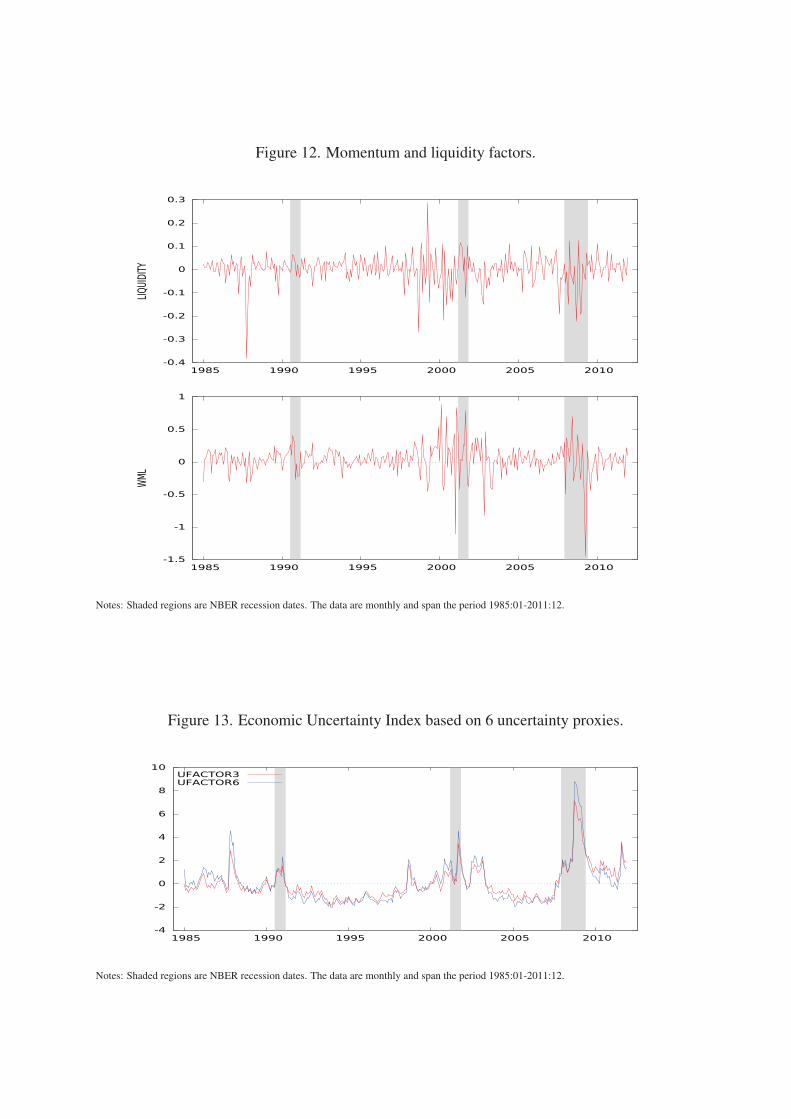
Figure 12. Momentum and liquidity factors.

��

��

��

��

��

��

��

��

��

� ��

��

��

��

��

��

��

��

��


Figure 13. Economic Uncertainty Index based on 6 uncertainty proxies.

��

��

��

��

��

��

��

��

��

��


References

[1] Abdymomunov, A., Morley, J. (2011). Time variation of CAPM betas across market volatility

regimes. Applied Financial Economics, 21, 1463-1478.

[2] Acharya, V.V., Pedersen, L.H. (2005). Asset pricing with liquidity risk. Journal of Financial

Economics, 77, 375-410.

[3] Anderson, E.W., Ghysels, E., Juergens, J.L. (2009). The impact of risk and uncertainty on expected

returns. Journal of Financial Economics, 94, 233-263.

[4] Ang, A., Hodrick, R.J., Xing, Y., Zhang, X. (2006). The cross-section of volatility and expected

returns. Journal of Finance, 61, 259-299.

[5] Ang, A., Timmermann, A. (2011). Regime changes and financial markets. Working paper No.

17182, NBER.

[6] Bachmann, R., Elstner, S., Sims, E. (2013). Uncertainty and economic activity: Evidence from

business survey data. American Economic Journal: Macroeconomics, 5, 217-249.

[7] Baker, S.R., Bloom, N., and Davis S.J. (2012). Measuring Economic Policy Uncertainty, Mimeo.

[8] Bakshi, G., Kapadia, N. (2003). Delta-hedged gains and the negative market volatility risk

premium. Review of Financial Studies, 16, 527-566.

[9] Bali, T.G., Engle, R.F. (2010). The intertemporal capital asset pricing model with dynamic

conditional correlations. Journal of Monetary Economics, 57, 377-390.

[10] Bali, T.G., Brown, S.J., Caglayan, M.O. (2014). Macroeconomic risk and hedge fund returns.

Journal of Financial Economics, forthcoming.

[11] Bali, T.G., Zhou, H. (2013). Risk, uncertainty, and expected returns. Working paper, Georgetown

University.

[12] Banerjee, P., Doran, J., Peterson, D.R. (2007). Implied volatility and future portfolio returns.

Journal of Banking and Finance, 31, 3183-3199.

[13] Bansal, R., Yaron, A. (2004). Risks for the long run: A potential resolution of asset pricing puzzles.

Journal of Finance, 59, 1481-1509.

[14] Banz, R.W. (1981). The relationship between return and market value of common stocks. Journal

of Financial Economics, 9, 3-18.

[15] Bekaert, G., Engstrom, E., Xing, Y. (2009). Risk, uncertainty, and asset prices. Journal of Financial

Economics, 91, 59-82.

[16] Bloom, N. (2009). The impact of uncertainty shocks. Econometrica, 77, 623-685.

[17] Bloom, N. (2013). Fluctuations in uncertainty. Working paper No 19714, NBER.

[18] Bloom, N., Bond, S., Van Reenen, J. (2007). Uncertainty and investment dynamics. Review of

Economic Studies, 74, 391-415.

[19] Bloom, N., Floetotto, M., Jaimovich, N., Saporta-Eksten, I., Terry, S.J. (2012). Really uncertain

business cycles. Working Paper No 18245, NBER.

[20] Bloom, N., Kose, M., Terrones, M. (2013). Held back by uncertainty. Finance and Development,

50, 38-41.

[21] Brogaard, J., Detzel, A. (2013). The asset pricing implications of government economic policy

uncertainty. Working paper, University of Washington.

[22] Campbell, J.Y. (1993). Intertemporal asset pricing without consumption data. American Economic

Review, 83, 487-512.

[23] Campbell, J.Y. (1996). Understanding risk and return. Journal of Political Economy, 104, 298-345.

[24] Chan, L.K.C., Jegadeesh, N., Lakonishok, J. (1996). Momentum strategies. Journal of Finance, 51,

1681-1713.

[25] Charles, A., Darné, O. (2014). Large shocks in the volatility of the Dow Jones Industrial Average

index: 1928-2013. Journal of Banking and Finance, 43, 188-199.

[26] Chen, L., Petkova, R., Zhang, L. (2008). The expected value premium. Journal of Financial

Economics, 87, 269-280.

[27] Chung, K.H., Chuwonganant, C. (2014). Uncertainty, market structure, and liquidity. Journal of

Financial Economics, forthcoming.

[28] De Bondt, W.F.M., Thaler, R.H. (1985). Does the stock market overreact? Journal of Finance, 40,

793-805.

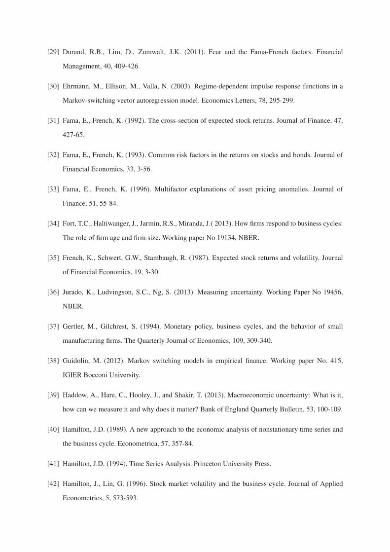
[29] Durand, R.B., Lim, D., Zumwalt, J.K. (2011). Fear and the Fama-French factors. Financial

Management, 40, 409-426.

[30] Ehrmann, M., Ellison, M., Valla, N. (2003). Regime-dependent impulse response functions in a

Markov-switching vector autoregression model. Economics Letters, 78, 295-299.

[31] Fama, E., French, K. (1992). The cross-section of expected stock returns. Journal of Finance, 47,

427-65.

[32] Fama, E., French, K. (1993). Common risk factors in the returns on stocks and bonds. Journal of

Financial Economics, 33, 3-56.

[33] Fama, E., French, K. (1996). Multifactor explanations of asset pricing anomalies. Journal of

Finance, 51, 55-84.

[34] Fort, T.C., Haltiwanger, J., Jarmin, R.S., Miranda, J.( 2013). How firms respond to business cycles:

The role of firm age and firm size. Working paper No 19134, NBER.

[35] French, K., Schwert, G.W., Stambaugh, R. (1987). Expected stock returns and volatility. Journal

of Financial Economics, 19, 3-30.

[36] Jurado, K., Ludvingson, S.C., Ng, S. (2013). Measuring uncertainty. Working Paper No 19456,

NBER.

[37] Gertler, M., Gilchrest, S. (1994). Monetary policy, business cycles, and the behavior of small

manufacturing firms. The Quarterly Journal of Economics, 109, 309-340.

[38] Guidolin, M. (2012). Markov switching models in empirical finance. Working paper No. 415,

IGIER Bocconi University.

[39] Haddow, A., Hare, C., Hooley, J., and Shakir, T. (2013). Macroeconomic uncertainty: What is it,

how can we measure it and why does it matter? Bank of England Quarterly Bulletin, 53, 100-109.

[40] Hamilton, J.D. (1989). A new approach to the economic analysis of nonstationary time series and

the business cycle. Econometrica, 57, 357-84.

[41] Hamilton, J.D. (1994). Time Series Analysis. Princeton University Press.

[42] Hamilton, J., Lin, G. (1996). Stock market volatility and the business cycle. Journal of Applied

Econometrics, 5, 573-593.

[43] Hamilton, J.D., Susmel, R. (1994). Autoregressive conditional heteroskedasticity and changes in

regime. Journal of Econometrics, 64, 307-33.

[44] Hess, M.K. (2003). What drives Markov regime-switching behavior of stock markets? The Swiss

case. International Review of Financial Analysis, 12, 527-43.

[45] Jagannathan, R., Wang, Z. (1996). The conditional CAPM and the cross-section of expected

returns. Journal of Finance, 51, 3-54.

[46] Jegadeesh, N., Titman, S. (1993). Returns to buying winners and selling losers: Implications for

stock market efficiency. Journal of Finance, 48 , 65-91.

[47] Jegadeesh, N., Titman, S. (2001). Profitability of momentum strategies: An evaluation of

alternative explanations. Journal of Finance, 56, 699-720.

[48] Jurado, K., Ludvigson, S.C., Ng, S. (2013). Measuring uncertainty. Working Paper No 19456,

NBER.

[49] Kim, C.J., Morley, J.C., Nelson, C.R. (2001). Does an intertemporal tradeoff between risk and

return explain mean reversion in stock prices? Journal of Empirical Finance, 8, 403-26.

[50] Kim, C.J., Morley, J.C., Nelson, C.R. (2004). Is there a positive relationship between stock market

volatility and the equity premium? Journal of Money, Credit, and Banking, 36, 339-60.

[51] Kim, C.J., Nelson, C.R., Startz, R. (1998). Testing for mean reversion in heteroskedastic data based

on Gibbs-sampling-augmented randomization. Journal of Empirical Finance, 5, 131-54.

[52] Knight, F.H. (1921). Risk, Uncertainty and Profit. Houghton Mifflin Co., Boston, MA.

[53] Korajczyk, R.A., Sadka, R. (2008). Pricing the commonality across alternative measures of

liquidity. Journal of Financial Economics, 87, 45-72.

[54] Krolzig, H.-M. (1997). Markov-Switching Vector Autoregressions: Modelling, Statistical

Inference, and Application to Business Cycle Analysis. Lecture Notes in Economics and

Mathematical Systems, Springer.

[55] Lee, K.-H. (2011). The world price of liquidity risk. Journal of Financial Economics, 99, 136-161.

[56] Lettau, M., Ludvigson, S. (2001). Resurrecting the (C)CAPM: a cross-sectional test when risk

premia are time-varying. Journal of Political Economy, 109, 1238-1287.

[57] Lintner, J. (1965). The valuation of risk assets and the selection of risky investments in stock

portfolio and capital budgets. Review of Economics and Statistics, 47, 13-37.

[58] Mayfield, E.S. (2004). Estimating the market risk premium. Journal of Financial Economics, 73,

465-96.

[59] Merton, R. (1980). On estimating the expected return on the market: An exploratory investigation.

Journal of Financial Economics, 8, 323-361.

[60] Mossin, J. (1966). Equilibrium in a capital asset market. Econometrica, 34, 768-783.

[61] Pastor, L., Stambaugh, R.F. (2003). Liquidity risk and expected stock returns. Journal of Political

Economy, 111, 642-685.

[62] Petkova, R., Zhang, L. (2005). Is value riskier than growth? Journal of Financial Economics, 78,

187-202.

[63] Reinganum, M.R. (1981). Misspecification of capital asset pricing: Empirical anomalies based on

earnings’ yields and market values. Journal of Financial Economics, 9, 19-46.

[64] Reinganum, M.R. (1982). A direct test of Roll’s conjecture on the firm size effect. Journal of

Finance, 37, 27-35.

[65] Schaller, H., van Norden, S. (1997). Regime switching in stock market returns. Applied Financial

Economics, 7, 177-91.

[66] Schwert, G.W. (1989). Business cycles, financial crises, and stock volatility. Carnegie-Rochester

Conference Series on Public Policy, 31, 83-126.

[67] Shamsuddin, A., Kim, J.H. (2008). Market sentiment and the Fama-French factor premia. Working

Paper.

[68] Sharpe, W. (1964). Capital asset prices: A theory of market equilibrium under conditions of risk.

Journal of Finance, 19, 425-42.

[69] Shih, Y-C., Chen, S-S., Lee, C-F., Chen, P-J. (2014). The evolution of capital asset pricing models.

Review of Quantitative Finance and Accounting, 42, 415-448.

[70] Verardo, M. (2009). Heterogeneous beliefs and momentum profits. Journal of Financial and

Quantitative Analysis, 44, 795U822.

[71] Veronesi, P. (1999) Stock market overreaction to bad news in good times: A rational expectations

equilibrium model. Review of Financial Studies, 12, 975-1007.

[72] Whaley, R.E. (2009). Understanding the VIX. Journal of Portfolio Management, 35, 98-105.

[73] Zhang, L. (2005). The value premium. Journal of Finance, 60, 67-103.

[74] Zhang, X.F. (2006). Information uncertainty and stock returns. Journal of Finance, 61, 105-137.

6 Appendix A: MSIAH(4)-VAR models

Table 6. Transition matrix for MSIAH(4)-VAR models

Regime 1 Regime 2

VXO Regime 1 0.8775 0.1225

Regime 2 0.0351 0.9649

UMACRO Regime 1 0.8788 0.1212

Regime 2 0.0282 0.9718

EPU Regime 1 0.8926 0.1074

Regime 2 0.0378 0.9622

UFACTOR Regime 1 0,8532 0,1468

Regime 2 0,0597 0,9403

7 Appendix B: MSIAH(5)-VAR models with liquidity factor

Figure 14. Estimated smoothed probabilities for MSIAH(5)-VAR(1) models with liquidity

factor.

1985 1990 1995 2000 2005 2010

0.5

1.0


Smoothed prob., Regime 2(a) with VXO

1985 1990 1995 2000 2005 2010

0.5

1.0


Smoothed prob., Regime 2(b) with EPU




3 6

−0.2

0

0.2Regime 1

Rm

−R

f

3 6

−0.2

0

0.2Regime 2

3 6−0.1

0

0.1

0.2

SM

B

3 6−0.1

0

0.1

0.2

3 6−0.2

−0.1

0

HM

L

3 6−0.2

−0.1

0

3 6−0.2

00.20.4

Liq

uid

ity

3 6−0.2

00.20.4

Note: Responses of the risk premia (Rm-Rf), SMB, HML and the liquidity factor to a positive shock to

VXO by one standard deviation. The impulse reaction period is chosen to be 6 months. Solid lines show

impulse responses, while dashed lines represent confidence intervals using the 10th and 90th percentile

values calculated on the basis of 1000 bootstrap replications.


3 6−0.1

−0.05

0

0.05Regime 1

Rm

−R

f

3 6−0.1

−0.05

0

0.05Regime 2

3 6−0.05

0

0.05

SM

B

3 6−0.05

0

0.05

3 6

−0.04

−0.02

0

0.02

HM

L

3 6

−0.04

−0.02

0

0.02

3 6

−0.050

0.050.1

Liq

uid

ity

3 6

−0.050

0.050.1


EPU by one standard deviation. The impulse reaction period is chosen to be 6 months. Solid lines show



8 Appendix C: MSIAH(5)-VAR model with momentum factor

Figure 17. Estimated smoothed probabilities for MSIAH(5)-VAR(1) models with

momentum factor.

1985 1990 1995 2000 2005 2010

0.5

1.0

Smoothed prob., Regime 2 (a) With VXO

1985 1990 1995 2000 2005 2010

0.5

1.0


Smoothed prob., Regime 2(b) With EPU

1985 1990 1995 2000 2005 2010

0.5

1.0

Smoothed prob., Regime 2(c) With UMACRO

1985 1990 1995 2000 2005 2010

0.5

1.0

Smoothed prob., Regime 2(d) With Factor 3

Note: the timeline of the figure indicates two regimes describing the sample period for different models.

Regime 1, corresponding to the high volatility regime, is represented over periods of 2000 to 2003, and

2008 to the end of 2012. For different estimations, MSIAH(5)-VAR(1) models contain the four risk

premia (Rm-Rf), SMB, HML and WML along with one of the uncertainty factors, namely, VXO, EPU,

UMACRO and Factor 3.

Figure 18. Response to VXO shock

3 6−0.2

0

0.2Regime 1

Rm

−R

f

3 6−0.2

0

0.2Regime 2

3 6−0.1

00.10.2

SM

B

3 6−0.1

00.10.2

3 6

−0.2

−0.1

0

0.1

HM

L

3 6

−0.2

−0.1

0

0.1

3 6−0.02

−0.01

0

0.01

WM

L

3 6−0.02

−0.01

0

0.01





Figure 19. Response to EPU shock

3 6−0.1

−0.05

0

0.05Regime 1

Rm

−R

f

3 6−0.1

−0.05

0

0.05Regime 2

3 6−0.05

0

0.05

SM

B

3 6−0.05

0

0.05

3 6

−0.04−0.02

00.02

HM

L

3 6

−0.04−0.02

00.02

3 6

024

x 10−3

WM

L

3 6

024

x 10−3





Figure 20. Response to UMACRO shock

3 6−0.2

−0.1

0

0.1Regime 1

Rm

−R

f

3 6

−0.2

−0.1

0

Regime 2

3 6−0.1

−0.05

0

0.05

SM

B

3 6−0.1

−0.05

0

0.05

3 6−0.1

−0.05

0

0.05

HM

L

3 6−0.1

−0.05

0

0.05

3 6−0.01

0

0.01

WM

L

3 6−0.01

0

0.01





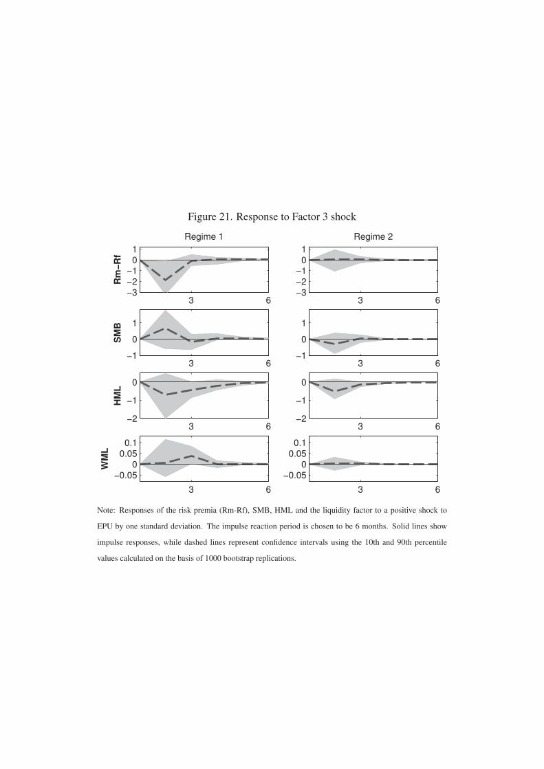
Figure 21. Response to Factor 3 shock

3 6−3−2−1

01

Regime 1

Rm

−R

f

3 6−3−2−1

01

Regime 2

3 6−1

0

1

SM

B

3 6−1

0

1

3 6−2

−1

0

HM

L

3 6−2

−1

0

3 6

−0.050

0.050.1

WM

L

3 6

−0.050

0.050.1





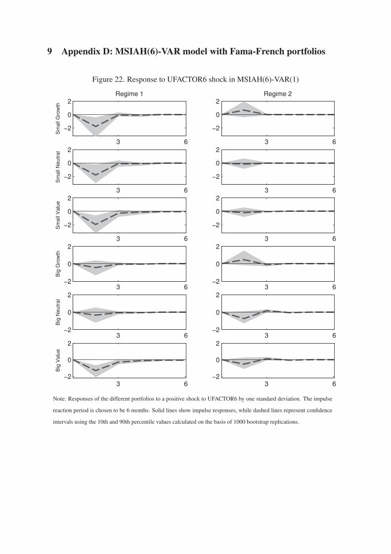
9 Appendix D: MSIAH(6)-VAR model with Fama-French portfolios


3 6

−2

0

2Regime 1

Sm

all

Gro

wth

3 6

−2

0

2Regime 2

3 6

−2

0

2

Sm

all

Neutr

al

3 6

−2

0

2

3 6

−2

0

2

Sm

all

Valu

e

3 6

−2

0

2

3 6−2

0

2

Big

Gro

wth

3 6−2

0

2

3 6−2

0

2

Big

Neutr

al

3 6−2

0

2

3 6−2

0

2

Big

Valu

e

3 6−2

0

2

Note: Responses of the different portfolios to a positive shock to UFACTOR6 by one standard deviation. The impulse

reaction period is chosen to be 6 months. Solid lines show impulse responses, while dashed lines represent confidence

intervals using the 10th and 90th percentile values calculated on the basis of 1000 bootstrap replications.

The sensitivity of Fama-French factors

to economic uncertainty

Online Technical Appendix

Abstract

This paper analyzes the sensitivity of the three Fama-French factors in relation to the US eco-

nomic uncertainty, by using three proxies of uncertainty measures in macroeconomics, financial

markets or economic policy from January 1985 to December 2011. We examine the extent, speed

and duration of response of the three (market, size and value) risk premia to movements in the

US uncertainties under low and high volatility regimes through the Markov-regime switching VAR

model. We find clearly two (high and low) volatility regimes, where each regime is highly persistent.

The high volatility regime is the prevailing regime between periods of 2000 to 2003, and 2008 to the

end of 2012. We show a negative effect of changes in financial and economic policy uncertainties on

value risk premia during the high volatility regime. This finding imply that investors move to growth

stocks from value stocks in high volatility regime when volatility is expected to increase. The latter

suggests that value firms can be more risky than growth firms during high volatility periods. We

also propose an aggregate measure of economic uncertainty by using Principal Component Analysis

based on the three uncertainty proxies. The results on value risk premia are confirmed. We find a

negative relationship between the market risk premium and the change in the economic uncertainty

index in high volatility regime. Finally, by adding a liquidity risk factor we find a positive effect of

financial uncertainty on liquidity factor during the high volatility regime, suggesting that investors

preferring liquidity stocks when market uncertainty increases.

Keywords: Fama-French factors; Economic uncertainty; Markov-switching model.

JEL Classification: G10; G11; C32.

1 Appendix A: MSIAH(4)-VAR models

1.1 MSIAH(4)-VAR(p) estimation results: VXO

Table 1. Linearity test: VAR model

Lags IC Two regimesa single regime

Lag1

AIC 20.1921* 21.1228

HQ 20.4823 * 21.2632

SC 20.9189* 21.4745

Lag2

AIC 20.3035* 21.1397

HQ 20.7445* 21.3555

SC 21.4079* 21.6802

Lag3

AIC 20.3558* 21.0405

HQ 20.9483* 21.3321

SC 21.8396* 21.7707

aAll information criterion (values with an

asterisk (*)) for all number of lags support the

presence of regime shifts.

Table 2. Lag length test: MSIAH(4)-VAR(p) model

AICa HQ SC

Lag = 1 20.1660* 20.3813* 20.7053*

Lag = 2 20.1940 20.4848 20.9224

Lag = 3 20.1991 20.5659 21.1177

aThe lag length supported by the IC (values

with an asterisk (*)) is one.

Table 3. Transition matrix

Regime 1a Regime 2

Regime 1 0.8775 0.1225

Regime 2 0.0351 0.9649

aNote that pi, j = Pr(st+1 = j|st = i)

1.2 MSIAH(4)-VAR(p) estimation results: UMACRO



Lag1

AIC 13.3697* 13.9413

HQ 13.6598* 14.0817

SC 14.0965* 14.2930

Lag2

AIC 13.5314* 13.9615

HQ 13.9723* 14.1773

SC 14.6358 14.5020*

Lag3

AIC 13.5449* 13.9674

HQ 14.1374* 14.2589

SC 15.0287 14.6975*

a All information criterion (values with an

asterisk (*)) for all number of lags support

the presence of regime shifts (except SC for

Lag=2,3).


AICa HQ SC

Lag = 1 13.3697* 13.6598* 14.0965 *

Lag = 2 13.5314 13.9723 14.6358

Lag = 3 13.5449 14.1374 15.0287




Regime 1a Regime 2

Regime 1 0.8788 0.1212

Regime 2 0.0282 0.9718


1.3 MSIAH(4)-VAR(p) estimation results: EPU



Lag1

AIC 23.6659* 24.3413

HQ 23.9561* 24.4817

SC 24.3927* 24.6929

Lag2

AIC 23.9631* 24.3711

HQ 24.4041* 24.5869

SC 25.0675 24.9115*

Lag3

AIC 23.9113* 24.3494

HQ 24.5038* 24.6410

SC 25.3950 25.0795*

aInformation criterion (values with an aster-

isk (*)) for all number of lags (except SC for

Lag=2,3) support the presence of regime shifts.


AICa HQ SC

Lag = 1 23.6328* 23.8481* 24.1721*

Lag = 2 23.8411 24.1320 24.5696

Lag = 3 23.8345 24.2013 24.7531




Regime 1a Regime 2

Regime 1 0.8926 0.1074

Regime 2 0.0378 0.9622


1.4 MSIAH(4)-VAR(p) estimation results: UFACTOR



Lag1

AIC 16,32949* 17,1329

HQ 16,6196* 17,2733

SC 17,0562* 17,4845

Lag2

AIC 16,5494* 17,1895

HQ 16,9903* 17,4053

SC 17,6538* 17,73

Lag3

AIC 16,8641* 17,1853

HQ 17,4566* 17,4768

SC 18,3479 17,9154*





AICa HQ SC

Lag = 1 16,3294* 16,6196* 17,0562*

Lag = 2 16,5494 16,9903 17,6538

Lag = 3 16,8641 17,4566 18,3479




Regime 1a Regime 2

Regime 1 0,8532 0,1468

Regime 2 0,0597 0,9403


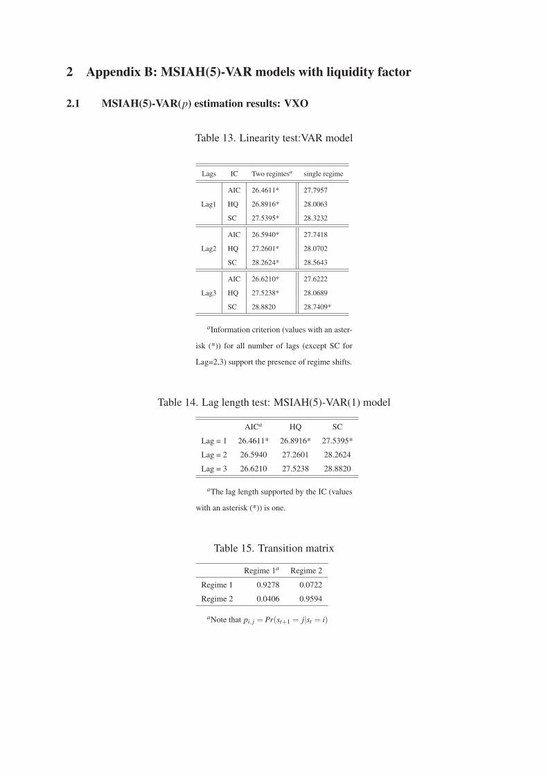
2 Appendix B: MSIAH(5)-VAR models with liquidity factor

2.1 MSIAH(5)-VAR(p) estimation results: VXO

Table 13. Linearity test:VAR model


Lag1

AIC 26.4611* 27.7957

HQ 26.8916* 28.0063

SC 27.5395* 28.3232

Lag2

AIC 26.5940* 27.7418

HQ 27.2601* 28.0702

SC 28.2624* 28.5643

Lag3

AIC 26.6210* 27.6222

HQ 27.5238* 28.0689

SC 28.8820 28.7409*




Table 14. Lag length test: MSIAH(5)-VAR(1) model

AICa HQ SC

Lag = 1 26.4611* 26.8916* 27.5395*

Lag = 2 26.5940 27.2601 28.2624

Lag = 3 26.6210 27.5238 28.8820




Regime 1a Regime 2

Regime 1 0.9278 0.0722

Regime 2 0.0406 0.9594


2.2 MSIAH(5)-VAR(p) estimation results: EPU

Table 16. Linearity test:VAR model


Lag1

AIC 30.0264* 31.0436

HQ 30.4569* 31.2542

SC 31.1048* 31.5711

Lag2

AIC 30.2903* 31.0579

HQ 30.9565* 31.3862

SC 31.9587* 31.8803

Lag3

AIC 30.3923* 31.0152

HQ 31.2951* 31.4619

SC 32.6533 32.1339*




Table 17. Lag length test: MSIAH(5)-VAR(1) model

AICa HQ SC

Lag = 1 30.0264* 30.4569* 31.1048*

Lag = 2 30.2903 30.9565 31.9587

Lag = 3 30.3923 31.2951 32.6533




Regime 1a Regime 2

Regime 1 0.9130 0.0870

Regime 2 0.0396 0.9604


Figure 1. Estimated smoothed probabilities for MSIAH(5)-VAR(1) models with liquidity

factor.

1985 1990 1995 2000 2005 2010

0.5

1.0


Smoothed prob., Regime 2(a) with VXO

1985 1990 1995 2000 2005 2010

0.5

1.0


Smoothed prob., Regime 2(b) with EPU

1985 1990 1995 2000 2005 2010

0.5

1.0


(c) With UMACRO

1985 1990 1995 2000 2005 2010

0.5

1.0

1.0


(d) With Factor 3




3 6

−0.2

0

0.2Regime 1

Rm

−R

f

3 6

−0.2

0

0.2Regime 2

3 6−0.1

0

0.1

0.2

SM

B

3 6−0.1

0

0.1

0.2

3 6−0.2

−0.1

0

HM

L

3 6−0.2

−0.1

0

3 6−0.2

00.20.4

Liq

uid

ity

3 6−0.2

00.20.4






3 6−0.1

−0.05

0

0.05Regime 1

Rm

−R

f

3 6−0.1

−0.05

0

0.05Regime 2

3 6−0.05

0

0.05

SM

B

3 6−0.05

0

0.05

3 6

−0.04

−0.02

0

0.02

HM

L

3 6

−0.04

−0.02

0

0.02

3 6

−0.050

0.050.1

Liq

uid

ity

3 6

−0.050

0.050.1






3 6−0.2

−0.1

0

Regime 1

Rm

−R

f

3 6−0.2

−0.1

0

Regime 2

3 6−0.1

0

0.1

SM

B

3 6−0.1

0

0.1

3 6−0.1

−0.05

0

0.05

HM

L

3 6−0.1

−0.05

0

0.05

3 6−0.2

−0.1

0

Liq

uid

ity

3 6−0.2

−0.1

0






3 6−3

−2

−1

0

Regime 1

Rm

−R

f

3 6−3

−2

−1

0

Regime 2

3 6−1

0

1

SM

B

3 6−1

0

1

3 6

−1.5−1

−0.50

0.5

HM

L

3 6

−1.5−1

−0.50

0.5

3 6

0

2

4

Liq

uid

ity

3 6

0

2

4





3 Appendix C: MSIAH(5)-VAR model with momentum factor

Figure 6. Estimated smoothed probabilities for MSIAH(5)-VAR(1) models with momen-

tum factor.

1985 1990 1995 2000 2005 2010

0.5

1.0

Smoothed prob., Regime 2 (a) With VXO

1985 1990 1995 2000 2005 2010

0.5

1.0


Smoothed prob., Regime 2(b) With EPU

1985 1990 1995 2000 2005 2010

0.5

1.0

Smoothed prob., Regime 2(c) With UMACRO

1985 1990 1995 2000 2005 2010

0.5

1.0

Smoothed prob., Regime 2(d) With Factor 3



2008 to the end of 2012. For different estimations, MSIAH(5)-VAR(1) models contain the four risk

premia (Rm-Rf), SMB, HML and WML along with one of the uncertainty factors, namely, VXO, EPU,

UMACRO and Factor 3.

Figure 7. Response to VXO shock

3 6−0.2

0

0.2Regime 1

Rm

−R

f

3 6−0.2

0

0.2Regime 2

3 6−0.1

00.10.2

SM

B

3 6−0.1

00.10.2

3 6

−0.2

−0.1

0

0.1

HM

L

3 6

−0.2

−0.1

0

0.1

3 6−0.02

−0.01

0

0.01

WM

L

3 6−0.02

−0.01

0

0.01

Note: Responses of the risk premia (Rm-Rf), SMB, HML and the momentum factor to a positive shock to




Figure 8. Response to EPU shock

3 6−0.1

−0.05

0

0.05Regime 1

Rm

−R

f

3 6−0.1

−0.05

0

0.05Regime 2

3 6−0.05

0

0.05

SM

B

3 6−0.05

0

0.05

3 6

−0.04−0.02

00.02

HM

L

3 6

−0.04−0.02

00.02

3 6

024

x 10−3

WM

L

3 6

024

x 10−3






3 6−0.2

−0.1

0

0.1Regime 1

Rm

−R

f

3 6

−0.2

−0.1

0

Regime 2

3 6−0.1

−0.05

0

0.05

SM

B

3 6−0.1

−0.05

0

0.05

3 6−0.1

−0.05

0

0.05

HM

L

3 6−0.1

−0.05

0

0.05

3 6−0.01

0

0.01

WM

L

3 6−0.01

0

0.01






3 6−3−2−1

01

Regime 1

Rm

−R

f

3 6−3−2−1

01

Regime 2

3 6−1

0

1

SM

B

3 6−1

0

1

3 6−2

−1

0

HM

L

3 6−2

−1

0

3 6

−0.050

0.050.1

WM

L

3 6

−0.050

0.050.1





4 Appendix D: MSIAH(6)-VAR model with Fama-French portfolios

Figure 11. Estimated smoothed probabilities for MSIAH(4)-VAR(1) models

1985 1990 1995 2000 2005 2010

0.5

1.0



(a) UFACTOR6 and small value portfolio

1985 1990 1995 2000 2005 2010

0.5

1.0



(b) UFACTOR6 and small neutral portfolio

1985 1990 1995 2000 2005 2010

0.5

1.0



(c) UFACTOR6 and small growth portfolio

1985 1990 1995 2000 2005 2010

0.5

1.0



(d) UFACTOR6 and big value portfolio

1985 1990 1995 2000 2005 2010

0.5

1.0



(e) UFACTOR6 and big neutral portfolio

1985 1990 1995 2000 2005 2010

0.5

1.0



(f) UFACTOR6 and big growth portfolio



2008 to the end of 2012.


3 6

−2

0

2Regime 1

Sm

all

Gro

wth

3 6

−2

0

2Regime 2

3 6

−2

0

2

Sm

all

Neutr

al

3 6

−2

0

2

3 6

−2

0

2

Sm

all

Valu

e

3 6

−2

0

2

3 6−2

0

2

Big

Gro

wth

3 6−2

0

2

3 6−2

0

2

Big

Neutr

al

3 6−2

0

2

3 6−2

0

2

Big

Valu

e

3 6−2

0

2

Note: Responses of the different portfolios to a positive shock to UFACTOR6 by one standard deviation. The impulse

reaction period is chosen to be 6 months. Solid lines show impulse responses, while dashed lines represent confidence

intervals using the 10th and 90th percentile values calculated on the basis of 1000 bootstrap replications.

Les Cahiers de la Chaire Finance rassemblent les documents de travail du LEMNA s'inscrivant dans des projets de recherche qu'elle soutient.

N° 2012-06 Are Islamic Indexes more Volatile than Conventional Indexes?

Evidence from Dow Jones Indexes CHARLES Amélie, DARNÉ Olivier et POP Adrian

N° 2012-07 Large Shocks in the Volatility of the Dow Jones Industrial Average

Index: 1928-2010 CHARLES Amélie et DARNÉ Olivier

N° 2012-08 The Quality of Private Monitoring in European Banking: Completing

the Picture POP Adrian et POP Diana

N° 2012-09 Effets socioéconomiques de la crise financière : implications pour le

Vietnam LAUZANAS Jean-Marc, PERRAUDEAU Yves et POP Adrian

N° 2012-31 Efficiency Gains from Narrowing Banks: A Search-Theoretic Approach TRIPIER Fabien

N° 2012-32 Volatility Persistence in Crude Oil Markets

CHARLES Amélie et DARNÉ Olivier

N° 2012-40 La modélisation en équilibre général et stochastique des cycles

économiques en Afrique Sub-saharienne : une revue de la littérature NOUASSI Claude Francis et TRIPIER Fabien

Les opinions exposées dans ce document n’engagent que les auteurs. Ceux-ci assument la responsabilité de toute

erreur ou omission.

La Chaire Finance est une initiative de la Banque Populaire Atlantique, la Caisse d’Epargne Bretagne-Pays de Loire, la

Caisse des Dépôts, du Crédit Maritime et de l’Université de Nantes, sous l’égide de la Fondation de Projets de

l’Université de Nantes.

Site web : http://www.univ-nantes.fr/fondation/chairefinance

Contact

Chaire Finance, Banque Populaire – Caisse d’Epargne IEMN-IAE, Chemin de Censive du Tertre – BP 52231

44322 Nantes cedex 3 Tél : +33 (0)2 40 14 16 60 Fax : +33 (0)2 40 14 16 50

Email : [email protected]

Les

Cah

iers

de

la C

hai

re F

inan

ce

W

ork

ing

Pap

er S

erie

s

N° 2012-41 The Dynamics of Gasoline Prices: Evidence from Daily French Micro

Data

GAUTIER Erwan et LE SAOUT Ronan N° 2014-07 Stock Exchange Mergers and Market Efficiency CHARLES Amélie, DARNÉ Olivier, KIM Jae et REDOR Etienne N° 2014-08 On the Relationship between the Prices of Oil and the Precious Metals:

Revisiting with a Multivariate Regime-Switching Decision Tree CHARLOT Philippe et MARIMOUTOU Vêlayoudom N° 2014-17 Precious metals shine? A market efficiency perspective CHARLES Amélie, DARNÉ Olivier et KIM Jae N° 2014-18 Sovereign bond yields in emerging Asia: New evidence PHAM Thi Hong Hanh N° 2014-19 Energy management systems and market value: Is there a link? PHAM Thi Hong Hanh N° 2014-20 The sensitivity of Fama-French factors to economic uncertainty CHARLES Amélie, DARNÉ Olivier et MOUSSA Zakaria

Les

Cah

iers

de

la C

hai

re F

inan

ce

W

ork

ing

Pap

er S

erie

s

The sensitivity of Fama-French factors to economic uncertainty

Documents

Transcript of The sensitivity of Fama-French factors to economic uncertainty