Evolution of biological Reaction Diffusion

Equations on various surfaces

by

Hannah WeinmannJonas Kleineisel

supervised by

Prof. Dr. Alfio Borzi

University of WurzburgAugust 2019

Abstract

We use ordinary differential equations to model populations of two interacting bio-logical species, mainly focussing on predator-prey systems. Confining our discussionto predator-prey systems with limit cycle behaviour, we subsequently add a spatialdimension to consider reaction-diffusion equations. This models spatial migrationof the two populations. We observe the emergence of spatial waves as a result ofthe population dynamics in combination with diffusion. Different boundary con-ditions for rectangular domains as well as the surface of a torus are considered.After shortly discussing an additonal convection term in the equation we turn ourattention to the sphere, which requires some more care to be directed towards thenumerical simulation. Many beautiful patterns arise from simulating different initialconditions on the sphere, which concludes our discussion.

Contents

1 Modelling of populations of two species with ODE’s 11.1 Lotka-Volterra equations . . . . . . . . . . . . . . . . . . . . . . . . . 11.2 Logistic growth . . . . . . . . . . . . . . . . . . . . . . . . . . . . . . 31.3 Symbiosis, competition and parasitic behavior . . . . . . . . . . . . . 31.4 Realistic predator-prey equations . . . . . . . . . . . . . . . . . . . . 5

2 Spatial Diffusion 92.1 Discretization and numerical method . . . . . . . . . . . . . . . . . . 92.2 Boundary conditions . . . . . . . . . . . . . . . . . . . . . . . . . . . 11

2.2.1 Dirichlet boundary condition . . . . . . . . . . . . . . . . . . 112.2.2 Neumann boundary condition . . . . . . . . . . . . . . . . . . 112.2.3 Torus boundary condition . . . . . . . . . . . . . . . . . . . . 12

3 Convection 18

4 Simulation on the Sphere 224.1 Discretization and numerical method . . . . . . . . . . . . . . . . . . 224.2 Results . . . . . . . . . . . . . . . . . . . . . . . . . . . . . . . . . . . 244.3 Conclusion and outlook . . . . . . . . . . . . . . . . . . . . . . . . . 29

Appendix 30

List of Figures 46

Bibliography 47

1 Modelling of populations of two species with

ODE’s

A classic example of modelling with ordinary differential equations are populationsizes of biological species, just think of the classical bacterial growth u′ = a u withsolution u(t) = u0 exp(at). Differential equations are well suited to model thesetypes of systems since, at least after making some (more or less realistic) assump-tions, the growth of a population is determined only by the current populationsize and some environmental factors like for example the amount of food available.From this one can often write down a differential equation describing a simplifiedversion of the mechanism of reproduction. A lot of information on this topic isgiven in [Mur04a]. However even when considering just one species, a lot of drasti-cally simplifying assumptions have to be made, to obtain a simple enough equation.Therefore, as always in modelling, one has to constantly weigh mathematical sim-plicity against realisticness.

1.1 Lotka-Volterra equations

The easiest type of model for biological populations is described by the well-knownLotka-Volterra equations

du

dt= u(1− v)

dv

dt= αv(u− 1)

where u represents the population of a species of prey and v that of of predatorsthat eat the prey. One assumes that in absence of predation, the prey just repro-duce exponentially. Additionally, the population of prey is controlled by predationwhich is proportional to the prey population size as well as the predator populationsize. The predators grow proportional to the predation term in the prey equationand in absence of prey just die exponentially for lack of food.

To avoid confusion the system of equations is given in the so-called nondimension-alized form. This means that through a series of subsitutions all variables havebeen normed and parameters expressed in relation to each other to obtain a mini-mal number of parameters. In this case the growth rate of the preys in absence ofpredators is normed to be 1 and the only remaining parameter is α > 0 describingthe relative growth rate of the predators to that of the prey.

Characteristic for Lotka-Volterra equations is the periodicity of the solutions. Forsome given initial condition, the solution in the phase plane plot is always a closedcurve on which the initial condition lies. At the same time, this is a major disad-vantage of this model, since any small perturbation will move the trajectory onto

1

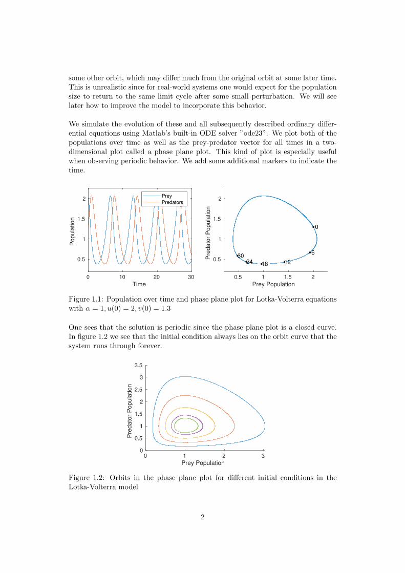
some other orbit, which may differ much from the original orbit at some later time.This is unrealistic since for real-world systems one would expect for the populationsize to return to the same limit cycle after some small perturbation. We will seelater how to improve the model to incorporate this behavior.

We simulate the evolution of these and all subsequently described ordinary differ-ential equations using Matlab’s built-in ODE solver ”ode23”. We plot both of thepopulations over time as well as the prey-predator vector for all times in a two-dimensional plot called a phase plane plot. This kind of plot is especially usefulwhen observing periodic behavior. We add some additional markers to indicate thetime.

0 10 20 30

Time

0.5

1

1.5

2

Po

pu

latio

n

Prey

Predators

0.5 1 1.5 2

Prey Population

0.5

1

1.5

2

Pre

da

tor

Po

pu

latio

n

0

6

12182430

Figure 1.1: Population over time and phase plane plot for Lotka-Volterra equationswith α = 1, u(0) = 2, v(0) = 1.3

One sees that the solution is periodic since the phase plane plot is a closed curve.In figure 1.2 we see that the initial condition always lies on the orbit curve that thesystem runs through forever.

0 1 2 3

Prey Population

0

0.5

1

1.5

2

2.5

3

3.5

Pre

dato

r P

opula

tion

Figure 1.2: Orbits in the phase plane plot for different initial conditions in theLotka-Volterra model

2

1.2 Logistic growth

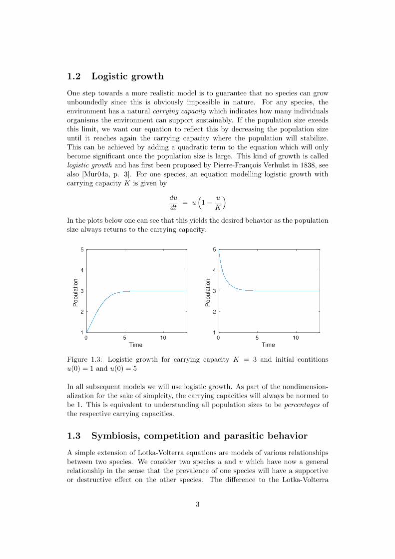
One step towards a more realistic model is to guarantee that no species can growunboundedly since this is obviously impossible in nature. For any species, theenvironment has a natural carrying capacity which indicates how many individualsorganisms the environment can support sustainably. If the population size exeedsthis limit, we want our equation to reflect this by decreasing the population sizeuntil it reaches again the carrying capacity where the population will stabilize.This can be achieved by adding a quadratic term to the equation which will onlybecome significant once the population size is large. This kind of growth is calledlogistic growth and has first been proposed by Pierre-Francois Verhulst in 1838, seealso [Mur04a, p. 3]. For one species, an equation modelling logistic growth withcarrying capacity K is given by

du

dt= u

(1− u

K

)In the plots below one can see that this yields the desired behavior as the populationsize always returns to the carrying capacity.

0 5 10

Time

1

2

3

4

5

Po

pu

latio

n

0 5 10

Time

1

2

3

4

5

Po

pu

latio

n

Figure 1.3: Logistic growth for carrying capacity K = 3 and initial contitionsu(0) = 1 and u(0) = 5

In all subsequent models we will use logistic growth. As part of the nondimension-alization for the sake of simplcity, the carrying capacities will always be normed tobe 1. This is equivalent to understanding all population sizes to be percentages ofthe respective carrying capacities.

1.3 Symbiosis, competition and parasitic behavior

A simple extension of Lotka-Volterra equations are models of various relationshipsbetween two species. We consider two species u and v which have now a generalrelationship in the sense that the prevalence of one species will have a supportiveor destructive effect on the other species. The difference to the Lotka-Volterra

3

equations is that both species can survive alone, while in the Lotka-Volterra modelthe predators can not subsist without prey. We assume that each species to exhibita logistic growth behavior in absence of the other species. Taking the symbiotic orcompetitive effect to be proportional to the population sizes of both species thisleads to the following equations:

du

dt= u (1− u+ av)

dv

dt= ρv (1− v + bu)

As discussed before, the system is nondimensionalized with both carrying capacitiesnormed to 1. The remaining parameters are:

ρ relative growth rate of species v in relation to growth rate of species ua coefficient determining the effect of species v on ub coefficient determining the effect of species u on v

For a, b > 0 we have symbiosis while for a, b < 0 we have competition. The caseswith mixed signs a < 0, b > 0 and a > 0, b < 0 could be interpreted as describingtwo species with one beeing a parasite to the other where one species is beneficialto the other species while having a negative effect on the other species.

0 5 10 15 20

t

0

0.5

1

1.5

Po

pu

latio

n

Competition

u

v

0 5 10 15 20

t

0

0.5

1

1.5

2

2.5

3

Po

pu

latio

n

Symbiosis

u

v

Figure 1.4: Competition with (ρ, a, b) = (1, -0.4, -0.6) and symbiosis with (ρ, a, b)= (0.4, 0.4, 0.6) and in both cases u(0) = 1.5, v(0) = 0.1

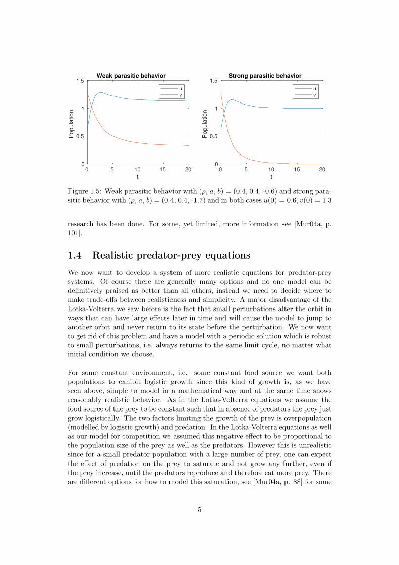
In these models, there is typically no perodic behavior as in the Lotka-Volterra equa-tions, instead the populations tend to stabilize after some time. One can clearlysee the effect of the interaction of the species on the steady states is to raise thelimit population in case of a positive effect and decrease it in case of a negativeeffect. In the parasitic case we see that if the negative effect that the parasite hason the other species is too great (b > 1), this species will die out and just leave theparasite which will then alone just behave in a logistic way.

It is not very hard to see how one can generalize this system of two species to asystem of n interacting species. On these types of systems with n > 3, not much

4

0 5 10 15 20

t

0

0.5

1

1.5

Po

pu

latio

nWeak parasitic behavior

u

v

0 5 10 15 20

t

0

0.5

1

1.5

Po

pu

latio

n

Strong parasitic behavior

u

v

Figure 1.5: Weak parasitic behavior with (ρ, a, b) = (0.4, 0.4, -0.6) and strong para-sitic behavior with (ρ, a, b) = (0.4, 0.4, -1.7) and in both cases u(0) = 0.6, v(0) = 1.3

research has been done. For some, yet limited, more information see [Mur04a, p.101].

1.4 Realistic predator-prey equations

We now want to develop a system of more realistic equations for predator-preysystems. Of course there are generally many options and no one model can bedefinitively praised as better than all others, instead we need to decide where tomake trade-offs between realisticness and simplicity. A major disadvantage of theLotka-Volterra we saw before is the fact that small perturbations alter the orbit inways that can have large effects later in time and will cause the model to jump toanother orbit and never return to its state before the perturbation. We now wantto get rid of this problem and have a model with a periodic solution which is robustto small perturbations, i.e. always returns to the same limit cycle, no matter whatinitial condition we choose.

For some constant environment, i.e. some constant food source we want bothpopulations to exhibit logistic growth since this kind of growth is, as we haveseen above, simple to model in a mathematical way and at the same time showsreasonably realistic behavior. As in the Lotka-Volterra equations we assume thefood source of the prey to be constant such that in absence of predators the prey justgrow logistically. The two factors limiting the growth of the prey is overpopulation(modelled by logistic growth) and predation. In the Lotka-Volterra equations as wellas our model for competition we assumed this negative effect to be proportional tothe population size of the prey as well as the predators. However this is unrealisticsince for a small predator population with a large number of prey, one can expectthe effect of predation on the prey to saturate and not grow any further, even ifthe prey increase, until the predators reproduce and therefore eat more prey. Thereare different options for how to model this saturation, see [Mur04a, p. 88] for some

5

options. We use the term a uvu+d with some a, d > 0 to describe the predation. The

parameter a expresses the negative effect the predation has on the prey populationin relation to the positive effect the predation has on the predator population. Thisis, for large a the predators need to eat many prey to reproduce some amountwhile for small a the predators only need to eat few prey to experience the samegrowth. The parameter d prevents the predation from becoming infinitely largefor small prey population and additionally makes the equation more numericallystable. For the predators we want them to exhibit logistic growth for a constantenvironment, i.e. for a constant prey population. This is actually the same as sayingthe predators grow logistically with a carrying capacity depending monotonicallyon the prey population. We take the carrying capacity to be proportional and evenequal to the prey population.This leads to the following system of equations:

du

dt= u

((1− u)− a v

u+ d

)dv

dt= bv

(1− v

u

)The parameter b > 0 expresses the linear growth rate of the predators in relation tothat of the prey, at least while being away from limiting factors to the populationlike overpopulation and large predation. With b > 1 the predators reproduce fasterthat the prey while for b < 1 it is the other way around.

For the right parameter values, this system posesses a stable limit cycle. One canactually carry out a detailed analysis to determine precisely for which parametersthe system is unstable or admits a stable limit cycle. In the case of the systemhaving a stable limit cycle there is always an unstable equilibrium point encircled(in the phase plane plot) by the limit cycle. This kind of analysis however is not ourmain focus since we are mostly concerned with modelling and numerical simulation.For a detailed treatment of exactly our model equations see [Mur04a, p.88]. For us,it suffices to summarize that the system is always stable for a < 1

2 and for any larger

a we need b and d to be large enough, for example b > 1a or d > (a2 + 4a)

12 − (1 +a)

always suffices (see [Mur04a, p.91]).

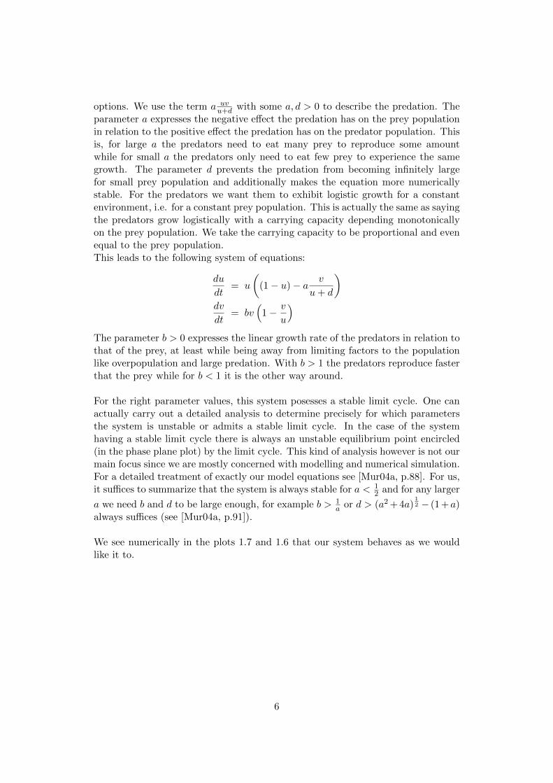
We see numerically in the plots 1.7 and 1.6 that our system behaves as we wouldlike it to.

6

0 50 100

Time

0

0.1

0.2

0.3

0.4

0.5

0.6

0.7

Po

pu

latio

n

Prey

Predators

0 0.2 0.4 0.6

Prey Population

0

0.1

0.2

0.3

0.4

0.5

Pre

da

tor

Po

pu

latio

n

0

20 40

60

80

100

Figure 1.6: Realistic predator-prey equation with a = 1, b = 0.5, d = 0.02 andu(0) = 0.5, v(0) = 0.5

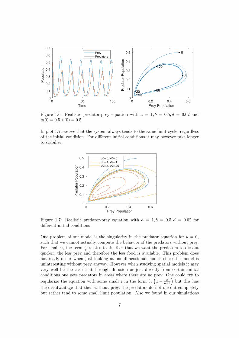
In plot 1.7, we see that the system always tends to the same limit cycle, regardlessof the initial condition. For different initial conditions it may however take longerto stabilize.

0 0.2 0.4 0.6

Prey Population

0

0.1

0.2

0.3

0.4

0.5

Pre

dato

r P

opula

tion

u0=.5, v0=.5

u0=.1, v0=.1

u0=.4, v0=.06

Figure 1.7: Realistic predator-prey equation with a = 1, b = 0.5, d = 0.02 fordifferent initial conditions

One problem of our model is the singularity in the predator equation for u = 0,such that we cannot actually compute the behavior of the predators without prey.For small u, the term u

v relates to the fact that we want the predators to die outquicker, the less prey and therefore the less food is available. This problem doesnot really occur when just looking at one-dimensional models since the model isuninteresting without prey anyway. However when studying spatial models it mayvery well be the case that through diffusion or just directly from certain initialconditions one gets predators in areas where there are no prey. One could try to

regularize the equation with some small ε in the form bv(

1− vu+ε

)but this has

the disadvantage that then without prey, the predators do not die out completelybut rather tend to some small limit population. Also we found in our simulations

7

this ε having to be rather large in order to have any regularizing effect if we didnot want to make the time step dt unresonably small. A more practical solutionis to program the simulation to set the predator population instantly to zero oncethe prey population falls below some small threshold. This does introduce somediscontinuity in the model but gets around the problem of residual populations andmakes it possible to work with initial conditions where there are no prey in someareas.

8

2 Spatial Diffusion

After analyzing the local interaction of population dynamics, we want to extendour model and add a spatial component. Since we assume that each animal of apopulation moves around in a random way we can think of the movement as adiffusion process. Equations that describe processes in which local interaction andadditional diffusion are linked, are called reaction diffusion systems. Mathematicallyseen such systems take the form of a parabolic partial differential equation of secondorder. We consider a two-dimensional spatial domain. The system of reactiondiffusion equations is given by

∂u∂t (x, y, t) = F (u(x, y, t), v(x, y, t)) +σprey (∆u)(x, y, t)∂v∂t (x, y, t) = G(u(x, y, t), v(x, y, t)) +σpredator (∆v)(x, y, t)

The functions u and v depend on the two space variables x, y and time t. Theydescribe the population dynamic of a predator-prey system. As before, u representsthe prey population and v the predator population.

The functions F and G describe the reaction and are given by the previously dis-cussed realistic predator-prey equations from chapter 1.4

F (u, v) = u

((1− u)− a v

u+ d

)G(u, v) = bv

(1− v

u

)whose parameters have already been explained there.

The terms σprey ∆u and σpredator ∆v describe the diffusion with diffusion coeffi-cients σspecies specific to the species. The diffusion coefficients indicate how fast thedispersion from a high to a low density takes place.

2.1 Discretization and numerical method

To solve our PDE numerically the function must be discretized. Consider a two-dimensional quadratic space of length L. Then the step size h is given by h =L

N−1 with N being the number of grid points. At each grid point (xi, yj) a valueis assigned that represents the population of the species. This value is denotedby u(xi, yj) respectively v(xi, yj). As time step size we use dt = T

M with T thetotal simulation time and M the number of time steps. From now on we discusseverything only for the preys u since everything goes analogous for the predators vanyway.

9

As an approximation for the derivative we use the explicit Euler method

∂

∂tu(x, y, t)

∣∣∣∣tk

≈ u(x, y, tk + dt)− u(x, y, tk)

dt

The second derivative can be approximated by

∂2

∂x2u(x, y, t) ≈ u(x+ h, y, t)− 2u(x, y, t) + u(x− h, y, t)

h2

This leads to

4u|(xi,yj) ≈u(xi+1, yj) + u(xi−1, yj)− 4u(xi, yj) + u(xi, yj+1) + u(xi, yj−1)

h2

Combined with the notation of u(xi, yj , tk) by uki,j the discrete reaction diffusionequation is then given by

uk+1i,j − uki,j

dt= F (uki,j , v

ki,j) + σprey 4 u|(xi,yj)

with k ∈ 1, ...,M and i, j ∈ 1, ..., N. Conversion leads to the iteration formula

uk+1i,j = uki,j + dt F (uki,j , v

ki,j) + dt σprey 4 u|(xi,yj)

As we have seen in the previous chapter, for the right parameter values the systemof realistic predator-prey equations possesses a stable limit cycle. By maintainingthese parameters for the reaction diffusion equation the question arises, what kindof spatial pattern formation can possibly occur. Of course this depends on thechosen initial conditions, for which one can for instance pick a Gaussian distribu-tion. This choice is particularly reasonable since the special case of no preys, whoseproblems were discussed above, does not arise. But of course other choices for theinitial conditions are possible.

In order to obtain a stable algorithm, it is important to analyze which stabilityconditions must be satisfied to get a well-conditioned problem. Since our mainfocus is not on the derivation of the stability condition, we only want to state thatsuch a condition is relevant and in our case it must hold σ dt

h2 < 1. However thiscondition is merely necessary and by no means sufficient, since even for very smallvalues of σ dt

h2 the numerical computation can fail due to numerical errors.

10

2.2 Boundary conditions

In the interior of the grid, the values uk+1i,j are well-defined by the above method

with given initial conditions, but not at the boundaries. These grid points mustbe manually adjusted and are called boundary conditions for which different valuescan be chosen. In the following three different possibilities for the prey populationare presented, which can be applied analogously to the predators.

2.2.1 Dirichlet boundary condition

In case of Dirichlet boundary conditions, the boundary values are set equal to zero,this means

u(x1, yj) = 0, u(xN , yj) = 0 for all j = 1, ..., N

u(xi, y1) = 0, u(xi, yN ) = 0 for all i = 1, ..., N

The figure 2.1 shows a simulation with Dirichlet boundary conditions. As initialvalues for both populations a Gaussian distribution with the position of the centercprey = (0.3, 0.3) and cpredator = (0.2, 0.2), height hprey = 0.5 and hpredator = 0.25,and standard deviation dprey = 0.1 and hpredator = 0.1 is chosen. As diffusioncoefficient we choose σ = 0.0001 for both populations.An advantage of Dirichlet boundary conditions is that they are easy to compute.One could say, that this model illustrates island populations, that can not leave theisland, or other szenarios where the species propagation is limited by untraversableboundaries.

2.2.2 Neumann boundary condition

A similar idea like Dirichlet boundary conditions is to consider smoother boundaryvalues. So instead of setting them to zero, in case of Neumann boundary conditions,the boundary values are set as the next inner point value, this means not thefunction values are predefined, but the derivative on the boundary of the grid is setto zero, i.e.

u(x1, yj) = u(x2, yj), u(xN , yj) = u(xN−1, yj) for all j = 1, ..., N

u(xi, y1) = u(xi, y2), u(xi, yN ) = u(xi, yN−1) for all i = 1, ..., N − 1

The value of the corner points u(x1, y1), u(x1, yN ), u(xN , y1), u(xN , yN ) doesn’tmatter, because for the computation of uk+1

i,j by the approximated reaction diffusionmethod the corner points are not involved.Figure 2.2 shows a simulation with Neumann boundary conditions. As initial con-ditions and diffusion coefficient the same values as in the Dirichlet case are chosen.If you compare the Neumann simulation to the Dirichlet simulation one can see,that they are not very different from each other in the interior.

11

2.2.3 Torus boundary condition

Until now we considered a bounded rectangular with untraversable boundaries. Toensure a propagation in every direction the idea is to build a torus by folding theorigin plane along the x and y axis. This means that plotted in two dimensions theleft and right boundary are the same and equivalently the bottom an top boundary.In conclusion in case of torus boundary conditions for the initial values holds

u(xi, y1) = u(xj , yN ) ∀ i = 1, ..., N

u(x1, yj) = u(xN , yj) ∀ j = 1, ..., N

To ensure that the initial condition satisfies the voundary condition the initial valuesare set as the mean value between the two nearest points, i.e.

u(xi, y1) =1

2(u(xi, y2) + u(xi, yN−1)) ∀ i = 1, ..., N

u(x1, yj) =1

2(u(x2, yj) + u(xN−1, yj)) ∀ j = 1, ..., N

This means that the initial corner points must be equal. It follows

u(x1, y1) =1

8(u(x2, y1) + u(x1, y2) + u(xN − 1, y1) + u(xN , y2)

+ u(x1, yN−1) + u(x2, yN ) + u(xN−1, yN ) + u(xN , yN−1))

u(x1, y1) = u(x1, yN ) = u(xN , y1) = u(xN , yN )

Figure 2.3 shows a simulation with Torus boundary conditions. As initial conditionsand diffusion coefficient the same values as in the Dirichlet and Neumann caseare chosen. One can see, that the waves are spreading over the edge, creating acompletely different pattern as in the first two cases.Since in the case of Torus boundary conditions the populations are considered on atorus, this of course leads to the idea of plotting the populations on a torus. To thisend we implemented by another plot function. The disadvantage of such a plot styleis that a large part is not visible and the propagation can not be comprehended sowell. The next figure 2.4 shows a simulation on a torus and figure 2.5 shows thesame simulation in a two dimensional plane plot as before.

12

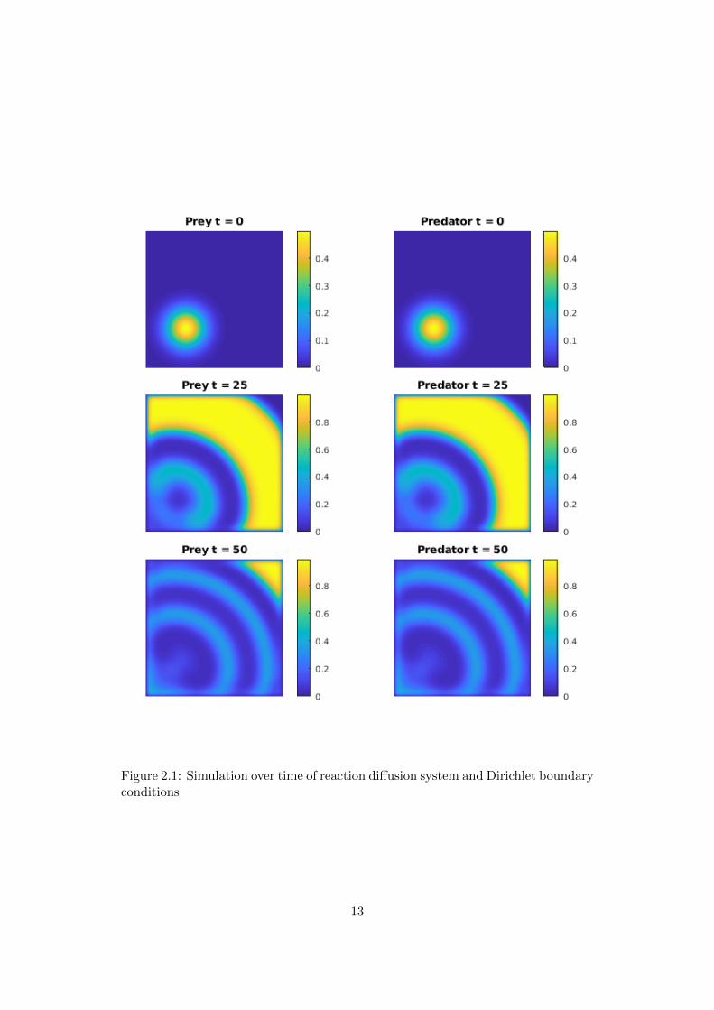
Figure 2.1: Simulation over time of reaction diffusion system and Dirichlet boundaryconditions

13

Figure 2.2: Simulation over time of reaction diffusion system and Neumann bound-ary conditions

14

Figure 2.3: Simulation over time of reaction diffusion system and Torus boundaryconditions

15

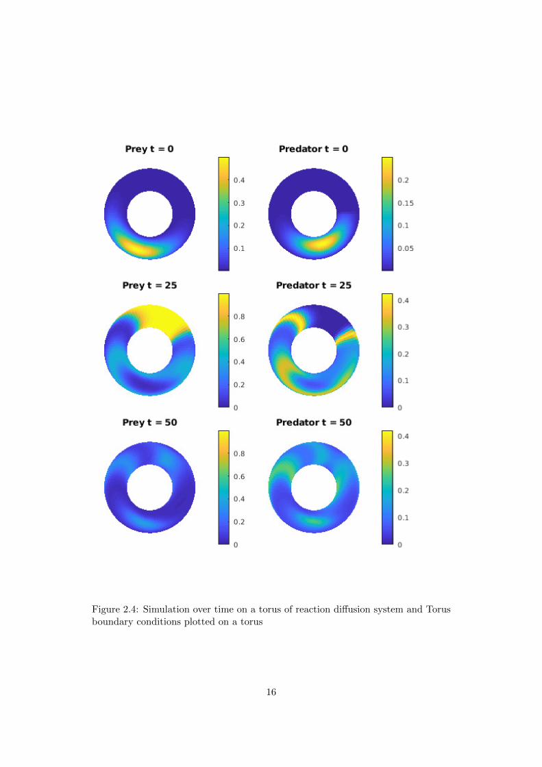
Figure 2.4: Simulation over time on a torus of reaction diffusion system and Torusboundary conditions plotted on a torus

16

Figure 2.5: Simulation over time on a plane of reaction diffusion system and Torusboundary conditions as a planar plot

17

3 Convection

So far our only spatial effect was diffusion, which, as we saw, can be regarded as aconstant drive in the system to equalize the population density in space. Anotherphysical possibility is a force acting (constant in time) on the species. This can beisotropic, meaning the force vector field is constant in space, or anisotropic. Objectssubjected to force of course resist this force in a way proportional to their mass.Here we interpret the population density as mass. If we imagine an isotropic con-vection to be similar to wind blowing things in some direction, then this basicallyjust means that low concentrations are blown away easily while larger amounts areharder to displace.

If the convection force is represented by a vector field ϕ : Ω → R2, then the effectof convection can be modelled by adding the convection term ϕ · ∇u to the par-tial differential equation. We thus obtain a system of reaction-diffusion-convectionequations:

∂u∂t = F (u, v) − cprey ϕ · ∇u +σprey∆u∂v∂t = G(u, v) − cpredator ϕ · ∇v +σpredator∆v

We always take the same convection force to act on both predators and prey, butwe allow for different convection speeds for the species, i.e. we rescale ϕ by a fac-tor cspecies. One could also consider completely different convection fields for thedifferent species.

For the numerical simulation we take the forward Euler method to approximate thederivative. This leaves us with the choice to take the forward difference ∂u

∂x

∣∣(i,j)≈

1h(u(i+1,j) − u(i,j)) or the backward difference ∂u

∂x

∣∣(i,j)

≈ 1h(u(i,j) − u(i−1,j)). To

increase stability, we always take the one, in which the convection direction for thex-component ϕx goes, i.e. for ϕx > 0 we take the forward difference and for ϕx < 0we take the backward difference. We use the expression

∂u

∂x

∣∣∣∣(i,j)

≈ max(0, ϕx)

(1

h(u(i,j) − u(i−1,j))

)+ min(0, ϕx)

(1

h(u(i+1,j) − u(i,j))

)to encapsulate this behavior. Everything goes analogous for ∂u

∂y , ∂v∂x and ∂v

∂y of course.

Concerning the numerical simulation, it is very noticable, how the simulation be-comes significantly less stable. Even for moderate convection speeds one has toreduce the time step dt by a large factor. Of course this has the consequence ofincreasing the computation time considerably and only allowing small simulationtimes T. But for too large time steps the numerics is so inaccurate that in areaswhere there are only small populations the population becomes negative, whichmakes no sense. If decreasing dt is not an option one could always counteract thisproblem by cutting the solution at 0 in every step, which means to always assign at

18

least 0 as population everywhere. While this significantly increases stability it alsodistorts the solution in ways not intended by the model and generates numericalsolutions which may deviate from actual solutions to the PDE arbitrarily much.Therefore we refrain from cutting and instead use small time steps and initial con-ditions that are easier to simulate.

We consider two examples, both with Neumann boundary condition. As an examplefor isotropic convection we take the constant convection direction (−1, 0)T , convec-tion speeds cprey = 1, cpredator = 0.01 and diffusion speeds σprey = 0.00001, σpredator =0.02. This results in the dynamics shown in figure 3.1. Notice how the movementof the prey is almost exclusively driven by convection due to their high convectionand low diffusion speed.

For anisotropic convection we consider a circular swirl around the center (L2 ,L2 )

of the domain. This means that the center remains fixed while any point (i, j)experiences convection with the vector field

ϕ(i, j) =

(−j + L

2

i− L2

).

The parameters we use here are convection speeds cprey = 1, cpredator = 0.1 anddiffusion speeds σprey = 0.00001, σpredator = 0.02. We see nicely in figure 3.2 howthe prey, due to their high convection speed, get pulled in a swirl around the center.The predators have a significantly lower convection speed but we can still make otthe deformation the convection has on the predator population.

19

Figure 3.1: Isotropic convection with convection direction ϕ = (−1, 0)T and con-vection speeds cprey = 1, cpredator = 0.01

20

Figure 3.2: Circular convection with convection speeds cprey = 1, cpredator = 0.1

21

4 Simulation on the Sphere

We will now disregard convection and return to our reaction-diffusion equation

∂u∂t = F (u, v) +σprey∆u∂v∂t = G(u, v) +σpredator∆v

with

F (u, v) = u

((1− u)− a v

u+ d

)G(u, v) = bv

(1− v

u

).

for u, v : Ω× [0, T ]→ R. So far, we discussed a quadratic spatial domain Ω = [0, L]2

with different boundary conditions. Now, we want to take the sphere Ω = r S2 ⊆ R3

for some fixed radius r > 0 as spatial domain.

4.1 Discretization and numerical method

The natural choice for coordinates are spherical coordinates with latitude ϑ ∈ [0, π),longitude ϕ ∈ [0, 2π) and radius r. To write the equation in spherical coordinateswe need to transform the Laplace operator from the usual cartesian coordinates tospherical coordinates. Using the transformation

x = r sinϑ cosϕ

y = r sinϑ sinϕ

z = r cosϑ

we obtain the Laplacian in spherical coordinates

∆u =∂2u

∂x2+∂2u

∂y2+∂2u

∂z2=

=1

r2∂

∂r

(r2∂u

∂r

)+

1

r2 sinϑ

∂

∂ϑ

(sinϑ

∂u

∂ϑ

)+

1

r2(sinϑ)2∂2u

∂ϕ

To discretize the sperical coordinates we define a N1 ×N2 grid by discretizing thelongitude ϕ ∈ [0, 2π) into N1 − 1 and the latitude ϑ ∈ [0, π) into N2 − 1 steps, i.e.we set

ϕi :=(i− 1)2π

(N1 − 1)∀i = 1, ..., N1

ϑj :=(j − 1)π

(N2 − 1)∀j = 1, ..., N2

22

resulting in step sizes

dϕ =2π

(N1 − 1)dϑ =

π

(N2 − 1).

Note that this way of discretizing the sphere has the disadvantage of distortingareas and lengths, since in very high or very low latitudes, one step in the longi-tude or the latitude direction constitutes a significantly shorter distance than at theequator. For the same reason one square in the grid near the poles has a smallerarea than one square around the equator. We treat it though, as if every step in thediscretization has the same physical length by treating every gridpoint equally inthe diffusion. This has the effect of slowing diffusion around the poles and speedingit up near the equator. There are better ways of discretizing a sphere. It is how-ever really simple to work with this discretization, which is why we prefer it for now.

We discretize time by specifying a simulation time T and a number of time stepsM , resulting in a time step

dt :=T

M.

We treat only the prey function u : rS2 × [0, T ]→ R but handle the predators v inexactly the same way. We set

ui,j,k := u(r, ϕi, ϑj , k dt) for k = 1, ...,M

for abbreviation since u depends on both space dimensions as well as time but theradius is constant anyway.

Using the forward Euler method with forward differences in space we proceed todiscretize the Laplacian in spherical coordinates

∆u|(i,j,k) =1

r2 sinϑ

∂

∂ϑ

(sinϑ

∂u

∂ϑ

)∣∣∣∣(i,j,k)

+1

r2(sinϑ)2∂2

∂ϕ2

∣∣∣∣(i,j,k)

=

=1

r2 sinϑi,j,k dϑ

(sinϑ

∂u

∂ϑ

∣∣∣∣(i,j+ 1

2,k)

− sinϑ∂u

∂ϑ

∣∣∣∣(i,j− 1

2,k)

)+

+1

r2(sinϑj)2(dϕ)2(ui+1,j,k − 2ui,j,k + ui−1,j,k) =

=1

r2 sinϑj (dϑ)2

(ui,j+1,k sinϑi,j+ 1

2,k − ui,j,k(sinϑi,j+ 1

2,k + sinϑi,j− 1

2,k)+

+ui,j−1,k sinϑi,j− 12,k

)+

1

r2(sinϑj)2(dϕ)2(ui+1,j,k − 2ui,j,k + ui−1,j,k)

by using

sinϑ∂u

∂ϑ

∣∣∣∣(i,j+ 1

2,k)

≈ sinϑj+ 12

uj+1 − ujdϑ

sinϑ∂u

∂ϑ

∣∣∣∣(i,j− 1

2,k)

≈ sinϑj− 12

uj − uj−1dϑ

23

Since we work on a sphere where the radius is constant, we have ∂u∂r = 0 and thus

can omit the first term in the spherical Laplacian.

For time differentiation we use the explicit Euler method

ui,j,k+1 − ui,j,kdt

= F (ui,j,k) + σ ∆u|i,j,k

In summary, the update formula for the simulation is

ui,j,k+1 = ui,j,k + dt F (ui,j,k) + dt σ ∆u|i,j,k ∀i = 1, ..., N1 − 1, j = 2, ..., N2 − 1

with ∆u|i,j,k given above. Since the longitudes ϕ = 0 and ϕ = 2π both correspondto zero-meridian, we have to set

uN1,j,k := u1,j,k ∀ j = 1, ..., N2

at every time step. Note also that for i = 1 we have to replace ui−1,j,k in the discretelaplacian by uN1−1,j,k in the discrete laplacian since ui−1,j,k is not well-defined fori = 1.

This leaves only the update behavior for the poles (j = 1 and j = N2) to bediscussed. At the north pole for example, i.e. j = N2, we can not meaningfully saywhat an ”eastern” neighbour ui+1,j,k should be, since at the north pole we can gonowhere but south. Since all points with j = N2−1 are neighbours, it is reasonableto instead of the four adjacent neighbour we consider all points with j = N2− 1 forthe diffusion and take the mean of all those values as replacement for the laplacian.This means, we update the north pole via

ui,N2,k+1 = F (u1,N2,k) + dt σ

N1∑i=1

ui,N2,k

N2

and analogously the south pole j = 1.

This concludes the description of our numerical method for the simulation of reaction-diffusion equations on the sphere. Additional information concerning the numericalsolution of differential equations on the sphere with more advanced methods canalso be found in [Bar89].

4.2 Results

With the method described above, we can generate many beautiful pictures. As ini-tial conditions we limit ourselves to taking two Gauss curves with different centersand standard deviations. As already in the planar case, we see the emergence ofspatial waves as a result of the population dynamics in combination with diffusion.But now, the waves traverse aroung the globe and interact with themselves. Thiscan be nicely seen in figure 4.2.

24

Another example is given in figure 4.3. In this simulation, we chose the diffusionspeeds by a factor of 10−2 lower than in figure 4.2. Therefore, the waves have muchmore defined edges and travel slower. If one looks closely, one can see how the wavefront of the preys is always a little bit ahead of the wave of predators, which followsthem. It is rather astonishing to see this behavior of pursuit emerging from only afew partial differential equations.

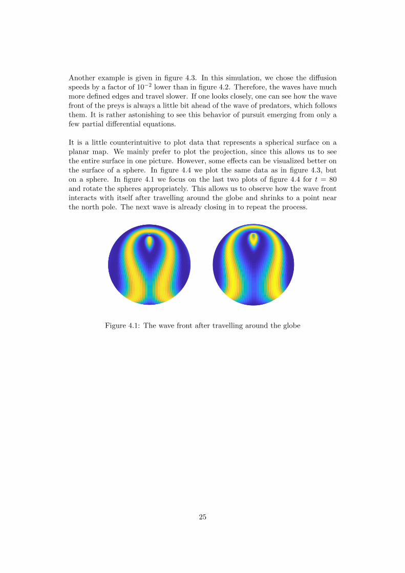
It is a little counterintuitive to plot data that represents a spherical surface on aplanar map. We mainly prefer to plot the projection, since this allows us to seethe entire surface in one picture. However, some effects can be visualized better onthe surface of a sphere. In figure 4.4 we plot the same data as in figure 4.3, buton a sphere. In figure 4.1 we focus on the last two plots of figure 4.4 for t = 80and rotate the spheres appropriately. This allows us to observe how the wave frontinteracts with itself after travelling around the globe and shrinks to a point nearthe north pole. The next wave is already closing in to repeat the process.

Figure 4.1: The wave front after travelling around the globe

25

Figure 4.2: Simulation of two Gauss curves on the sphere with σprey = 0.001,σpredator = 0.0001

26

Figure 4.3: Simulation of two Gauss curves on the sphere with σprey = 0.00001,σpredator = 0.000001

27

Figure 4.4: Simulation of two Gauss curves on the sphere with σprey = 0.00001,σpredator = 0.000001 as a spherical plot

28

4.3 Conclusion and outlook

One could argue that choosing a sphere as spatial domain is a natural choice, con-sidering that we and every form of life we know about lives on the spherical surfaceof the earth. Yet, the realisticness is still doubtful since no organism let alone a sys-tem of predators and prey could possibly diffuse around the entire globe due to forexample oceans or landmasses and other environmental factors like different climatezones. An attempt could be made to incorporate effects like these by, for exampletaking the diffusivities σ dependant on space to model areas like oceans, where nomigration is possible or areas like mountains where migration is aggravated. Alsothe parameters in the reaction term could be taken to depend on space to modeldifferent climate zones where animals reproduce differently or can not survive at alllike for example deserts. With all these effects incorporated, the numerical effortto simulate such a model on an at least somewhat realistic map of the earth wouldbe enormous. And even then is the real world much, much to complicated to besqueezed into a handful of equations. There is after all still an unresolvable conflictbetween realisticness and computability. Nevertheless the pictures generated aboveare very beautiful and the techniques could be used for some other equation on thesphere with more practical value.

29

Appendix

To help readers reproduce our results, we collected here some representative Matlab- codes for our simulations. Any plot we presented above can be generated by somestraightforward modifications of the following code.

Chapter 1

Since we use Matlab’s buit-in solver for ODE’s, the codes for the entire chapter arereally simple and can all be derived from the following example.

”codes/ODEs/simPredPreyReal.m”

% Numerical ly s o l v e s r e a l i s t i c predator−prey equat ions and% d i sp l a y s populat ion over time and phase plane p l o t

% so l v e d i f f e r e n t i a l equat ion numer i c a l l l y[ t , so lxy ] = ode23(@predPreyRealEq , [ 0 : 0 . 0 1 : 1 0 0 ] , [ 0 . 5 ; 0 . 5 ] ) ;f i g u r e ( ' Pos i t i on ' , [ 0 0 700 250 ] )newplot

% d i sp l ay populat ion over time p l o tsubplot (1 , 2 , 1)p l o t ( t , so lxy )x l ab e l ( 'Time ' )y l ab e l ( ' Populat ion ' )l egend ( 'Prey ' , ' Predators ' )yl im ( [ 0 0 . 7 1 ] )

% d i sp l ay phase plane p l o tsubplot (1 , 2 , 2)p l o t ( so lxy ( : , 1 ) , so lxy ( : , 2 ) )x l ab e l ( 'Prey Populat ion ' ) ;y l ab e l ( ' Predator Populat ion ' ) ;hold onylim ( [ 0 0 . 5 5 ] )

% add time l a b e l s to phase plane p l o ts t a r t t ime = 1 ;s tep = round ( l ength ( so lxy ) / 5) ;t ex t ( so lxy ( s t a r t t ime : s tep : end , 1 ) , so lxy ( s t a r t t ime : s tep : end , 2 ) , ...

num2str ( t ( s t a r t t ime : s tep : end ) ) ) ;s c a t t e r ( so lxy ( s t a r t t ime : s tep : end , 1 ) , so lxy ( s t a r t t ime : s tep : end , 2 ) , ...

5 , ”marker ” , ' o ' , ”marke r f aceco l o r ” , ' black ' , ”markeredgeco lor ” , ...' black ' ) ;

”codes/ODEs/predPreyRealEq.m”

% Rea l i s t i c predator−prey equat ionsfunc t i on dxdy = predPreyRealEq ( t , xy )

30

a = 1 ;b = 0 . 5 ;d = 0 . 0 2 ;dxdy=[((1−xy (1 ) )−a∗xy (2 ) /( xy (1 )+d) ) ∗xy (1 ) ; ( b∗(1−xy (2 ) /xy (1 ) ) ) ∗xy (2 ) ] ;end

Chapter 2

The simulation is implemented as described above. To visualize the results, we useMatlab’s surf function for both plot cases, the planar plot and the torus plot.

”codes/Spatial/simulationWithDirichlet.m”

f unc t i on s imu la t i onWithDi r i ch l e t ( )s imulat ionLotkaGenera l (@ comput eD i r i c h l e t I n i t i a l , ...@computeDirichletBoundary ) ;

end

”codes/Spatial/simulationWithNeumann.m”

f unc t i on simulationWithNeumann ( )s imulat ionLotkaGenera l (@computeNeumannInitial , ...@computeNeumannBoundary ) ;

end

”codes/Spatial/simulationWithTorus.m”

f unc t i on simulationWithTorus ( )s imulat ionLotkaGenera l (@computeTorusIn i t ia l ,@computeTorusBoundary ) ;

end

”codes/Spatial/simulationLotkaGeneral.m”

f unc t i on s imulat ionLotkaGenera l ( compute In i t i a l , computeBoundary )T = 50 ; % Simulat ion TimeM = 1000 ; % Number o f Time s t ep sN = 50 ; % Mesh S i z eL = 1 ; % Space S i z eh = L/(N−1) ; % Spa t i a l Stepdt = T/M; % Time Stepsigma = 0 . 0001 ; % D i f f u s i on c o e f f i c i e n t ( f o r both s p e c i e s )plotNumber = 3 ; % Number Of Plot s

% Generate I n i t i a l Condit ionu = ze ro s (N,N, 2 ) ;uplus = ze ro s (N,N, 2 ) ;uSavePlot = ze ro s (N,N, plotNumber , 2 ) ;

f o r i = 1 :N

31

f o r j = 1 :Nu( i , j , 1 ) = 1/(2) ∗ exp(−1/2 ∗ ( ( ( i ∗h−0.3) /0 . 1 ) ˆ2 +...( ( j ∗h−0.3) /0 . 1 ) ˆ2) ) ;u ( i , j , 2 ) = 1/(4) ∗ exp(−1/2 ∗ ( ( ( i ∗h−0.2) /0 . 1 ) ˆ2 +...( ( j ∗h−0.2) /0 . 1 ) ˆ2) ) ;

endend

%I n i t i a l boundary cond i t i onu = compute In i t i a l (u ) ;

uSavePlot ( : , : , 1 , : ) = u ( : , : , : ) ;

% Time loopf o r k = 1 :M

% Loop along x ax i sf o r i = 2 :N−1

% Loop along y ax i sf o r j = 2 :N−1

D i f f = squeeze ( ( u( i +1, j , : )+u( i −1, j , : )−4∗u( i , j , : )+...u ( i , j +1 , : )+u( i , j −1 , : ) ) /(h . ˆ 2 ) ) ;Reac = lotka2D ( squeeze (u( i , j , : ) ) ) ;uplus ( i , j , : )=squeeze (u( i , j , : ) )+dt∗Reac+dt∗ sigma∗Di f f ;i f ( i snan ( uplus ( i , j , 1 ) ) | | i snan ( uplus ( i , j , 2 ) ) )d i sp ( ' e r r o r nan ' ) ;r e turn

end

end

end% Computation o f Boundary va lue suplus = computeBoundary (u , uplus , dt , sigma , h) ;

u = uplus ;

f o r p = 1 : plotNumber −1i f k == f l o o r (p∗M/( plotNumber −1) )

uSavePlot ( : , : , p+1 , : ) = u ( : , : , : ) ;end

end

end

% Plot r e s u l t%plotGenera l (h , L , T, uSavePlot ) ;p lotTorus (T, uSavePlot ) ;

end

”codes/Spatial/computeDirichletInitial.m”

f unc t i on u = compu t eD i r i c h l e t I n i t i a l (u)[N,m, n ] = s i z e (u) ;u ( 1 , : , : ) = ze ro s (1 ,m, n) ;

32

u(N, : , : ) = u ( 1 , : , : ) ;u ( : ,N, : ) = u ( 1 , : , : ) ;u ( : , 1 , : ) = u ( 1 , : , : ) ;

end

”codes/Spatial/computeDirichletBoundary.m”

f unc t i on uplus = computeDirichletBoundary (u , uplus , dt , sigma , h)uplus = compu t eD i r i c h l e t I n i t i a l ( uplus ) ;

end

”codes/Spatial/computeNeumannInitial.m”

f unc t i on u = computeNeumannInitial (u )[N, ˜ , ˜ ] = s i z e (u) ;

u (N, : , : ) = u(N−1 , : , : ) ;u ( : ,N, : ) = u ( : ,N−1 , : ) ;u ( 1 , : , : ) = u ( 2 , : , : ) ;u ( : , 1 , : ) = u ( : , 2 , : ) ;

end

”codes/Spatial/computeNeumannBoundary.m”

f unc t i on uplus = computeNeumannBoundary (u , uplus , dt , sigma , h)uplus = computeNeumannInitial ( uplus ) ;

end

”codes/Spatial/computeTorusInitial.m”

f unc t i on u = computeTorus In i t ia l (u)[N, ˜ , ˜ ] = s i z e (u) ;f o r j = 2 :N−1

% Convolution around y ax i smidval = 0 .5 ∗ (u (2 , j , 1 )+u(N−1, j , 1 ) ) ;u (1 , j , 1 ) = midval ;u (N, j , 1 ) = midval ;midval = 0 .5 ∗ (u (2 , j , 2 )+u(N−1, j , 2 ) ) ;u (1 , j , 2 ) = midval ;u (N, j , 2 ) = midval ;

% Convolution around x ax i smidval = 0 .5 ∗ (u( j , 2 , 1 )+u( j ,N−1 ,1) ) ;u ( j , 1 , 1 ) = midval ;u ( j ,N, 1 ) = midval ;midval = 0 .5 ∗ (u( j , 2 , 2 )+u( j ,N−1 ,2) ) ;u ( j , 1 , 2 ) = midval ;u ( j ,N, 2 ) = midval ;

end% Corner computationu ( 1 , 1 , : ) = 1/8 ∗ (u ( 2 , 1 , : )+u(N−1 ,1 , : )+u ( 1 , 2 , : )+u (1 ,N−1 , : )+...

33

u (2 ,N, : )+u(N−1,N, : )+u(N,N−1 , : )+u(N, 2 , : ) ) ;u (1 ,N, : ) = u ( 1 , 1 , : ) ;u (N, 1 , : ) = u ( 1 , 1 , : ) ;u (N,N, : ) = u ( 1 , 1 , : ) ;

end

”codes/Spatial/computeTorusBoundary.m”

f unc t i on uplus = computeTorusBoundary (u , uplus , dt , sigma , h)[N, ˜ , ˜ ] = s i z e (u) ;% Torus boundary computationi = 1 ;f o r j = 2 :N−1

uplus = computeUPlus ( uplus , i , j ) ;endj = 1 ;f o r i = 2 :N−1

uplus = computeUPlus ( uplus , j , i ) ;end% Corner computationi = 1 ;j = 1 ;D i f f = squeeze ( ( u( i +1, j , : )+u(N−1, j , : )−4∗u( i , j , : )+u( i , j +1 , : )+...u ( i ,N−1 , : ) ) /(h . ˆ 2 ) ) ;Reac = lotka2D ( squeeze (u( i , j , : ) ) ) ;uplus ( i , j , : ) = squeeze (u( i , j , : ) ) + dt ∗ Reac + dt ∗ sigma ∗ Di f f ;

uplus (N, : , : ) = uplus ( 1 , : , : ) ;uplus ( : ,N, : ) = uplus ( : , 1 , : ) ;

uplus (1 ,N, : ) = uplus ( 1 , 1 , : ) ;uplus (N, 1 , : ) = uplus ( 1 , 1 , : ) ;uplus (N,N, : ) = uplus ( 1 , 1 , : ) ;

f unc t i on [ uplus ] = computeUPlus ( uplus , i , j )D i f f = squeeze ( ( u( i +1, j , : )+u(N−1, j , : )−4∗u( i , j , : )+...u ( i , j +1 , : )+u( i , j −1 , : ) ) /(h . ˆ 2 ) ) ;Reac = lotka2D ( squeeze (u( i , j , : ) ) ) ;uplus ( i , j , : ) = squeeze (u( i , j , : ) )+dt∗Reac+dt∗ sigma ∗ Di f f ;

endend

”codes/Spatial/plotGeneral.m”

f unc t i on p lotGenera l (h , L , T, uSavePlot )[X Y] = meshgrid ( 0 : h : L , 0 : h :L) ;[ ˜ , ˜ , plotNumber , ˜ ] = s i z e ( uSavePlot ) ;newplotf o r s p e c i e s = 1 :2

f o r i = 1 : plotNumbersubplot ( plotNumber , 2 , 2∗ ( i −1)+sp e c i e s ) ;hold on ;s u r f (X,Y, uSavePlot ( : , : , i , s p e c i e s ) , ' FaceColor ' , ' i n t e rp ' ) ;shading i n t e rp

34

hold o f f ;c = co l o rba r ;ax i s ( [ 0 L 0 L 0 1 ] ) ;ax i s square ;ax i s o f f ;

t = ( i −1)∗T/( plotNumber−1) ;i f ( s p e c i e s == 1)

t i t l e ( [ ' \ f o n t s i z e 6Prey t = ' , num2str ( t ) ] )e l s e

t i t l e ( [ ' \ f o n t s i z e 6Predator t = ' , num2str ( t ) ] )ends e t ( c , ' FontSize ' , 5 ) ;

view (2) ;end

endend

”codes/Spatial/plotTorus.m”

f unc t i on plotTorus (T, uSavePlot )

aminor = 1 . ; % Torus minor rad iu sRmajor = 3 . ; % Torus major rad iu s[ s1 , s2 , plotNumber , ˜ ] = s i z e ( uSavePlot ) ;

theta = l i n s p a c e (−pi , pi , s1 ) ; % Po lo ida l ang lephi = l i n s p a c e ( 0 . , 2 .∗ pi , s2 ) ; % Toro ida l ang le

[ t , p ] = meshgrid ( phi , theta ) ;

X = (Rmajor + aminor .∗ cos (p) ) .∗ cos ( t ) ;Y = (Rmajor + aminor .∗ cos (p) ) .∗ s i n ( t ) ;Z = aminor .∗ s i n (p) ;

newplotf o r s p e c i e s = 1 :2

f o r i = 1 : plotNumbersubplot ( plotNumber , 2 , 2∗ ( i −1)+sp e c i e s ) ;hold on ;s u r f (X,Y, Z , uSavePlot ( : , : , i , s p e c i e s ) ' , ' LineSty l e ' , ' none ' ) ;hold o f f ;c = co l o rba r ;ax i s square ;

ax i s o f f ;

t = ( i −1)∗T/( plotNumber−1) ;i f ( s p e c i e s == 1)

t i t l e ( [ ' \ f o n t s i z e 6Prey t = ' , num2str ( t ) ] )e l s e

t i t l e ( [ ' \ f o n t s i z e 6Predator t = ' , num2str ( t ) ] )ends e t ( c , ' FontSize ' , 5 ) ;

35

view (2) ;

endend

end

Chapter 3

The code for convection is similar to the codes used in chapter 2 with an addedconvection term. The convection force field is given as a function, allowing for easyswitching between different fields. For display, we additionally plot the convectionvector field using Matlab’s quiver3 plot.

”codes/Convection/main.m”

% Parametersplot number = 3 ; % Number o f P lo t s

% I s o t r o p i c Convection% M = 20000; % Number o f Time Steps% T = 1 . 1 ; % Simulat ion Time% N = 100 ; % Mesh S i z e% L = 1 ; % Space s i z e% sigma = [ 0 . 0 0 0 0 1 ; 0 . 0 1 ] ; % D i f f u s i on Speeds [ Prey , Predator ]% c = [ 1 , 0 . 0 1 ] ; % Convection speed [ Prey , Predator ]% %I n i t i a l Condit ion parameters% preyCenter = [ round (N/2)+10, round (N/2) ] ;% preySdtDev = 0 . 8 ;% preyM = 0 . 4 5 ;% predCenter = [ round (N/2)+5, round (N/2) ] ;% predSdtDev = 0 . 2 ;% predM = 1 ;% convec t i onF i e ld = @i so t r op i cConvec t i on ;

%Ci r cu l a r ConvectionM = 1000 ; % Number o f Time StepsT = 1 . 1 ; % Simulat ion TimeN = 30 ; % Mesh S i z eL = 1 ; % Space s i z esigma = [ 0 . 0 0 0 0 1 ; 0 . 0 2 ] ; % D i f f u s i on Speeds [ Prey , Predator ]c = [ 1 , 0 . 1 ] ; % Convection speed [ Prey , Predator ]%I n i t i a l Condit ion parameterspreyCenter = [ round (N/2)+10, round (N/2) ] ;preySdtDev = 0 . 8 ;preyM = 0 . 4 5 ;predCenter = [ round (N/2)+15, round (N/2) ] ;predSdtDev = 0 . 2 ;predM = 1 ;convec t i onF i e ld = @c i r cu l a rConvec t i on ;

% Generate I n i t i a l Condit ionh = L/(N−1) ;u = ze ro s (N, N, 2) ;

36

f o r i = 2 :N−1f o r j = 2 :N−1

u( i , j , 1 )=preyM∗exp(−(power (norm(h ∗ ( [ i , j ]−preyCenter ) ) /...preySdtDev , 2 ) ) ) ;

u ( i , j , 2 )=predM∗exp(−(power (norm(h ∗ ( [ i , j ]−predCenter ) ) /...predSdtDev , 2 ) ) ) ;

endend% Neumann boundary cond i t i on f o r i n i t i a l c ond i t i onu ( : , 1 , : ) = u ( : , 2 , : ) ;u ( : ,N, : ) = u ( : ,N−1 , : ) ;u ( 1 , : , : ) = u ( 2 , : , : ) ;u (N, : , : ) = u(N−1 , : , : ) ;% I n i t i a l Condit ion done

p l o t s = simConvection (u ,T,M,L ,N, convect ionFie ld , c , sigma , plot number ) ;

p laneConvect ionPlot ( p lo t s , T,L , convec t i onF i e ld ) ;

”codes/Convection/simConvection.m”

f unc t i on p l o t s = simConvection (u , T, M,L , ...N, convect ionFie ld , c , sigma , plot number )

dt = T / M;h = L/(N) ;

un = ze ro s (N, N, 2) ;uo = u ;

p l o t s = ze ro s (N,N, 2 , plot number ) ;p l o t s ( : , : , : , 1 ) = u ;

f o r k = 1 :Mf o r i = 2 :N−1

f o r j = 2 :N−1D i f f = squeeze ( ( uo ( i +1, j , : ) + uo ( i −1, j , : ) −...

4∗uo ( i , j , : ) + uo ( i , j +1 , : ) + uo ( i , j −1 , : ) ) /(h∗h) ) ;Reac = lotka2D ( squeeze ( uo ( i , j , : ) ) ) ;

phi = convec t i onF i e ld ( i , j , L , N) ;

% f o r phi (1 ) < 0 take (u( i +1, j , : ) − u( i , j , : ) ) ∗(1/h) and% f o r phi (1 ) > 0 take (u( i , j , : ) − u( i −1, j , : ) ) ∗(1/h)Conv = max(0 , phi (1 ) ) ∗ (u( i , j , : ) − u( i −1, j , : ) ) ∗(1/h)...

+ min (0 , phi (1 ) ) ∗ (u( i +1, j , : ) − u( i , j , : ) ) ∗(1/h) + ...max(0 , phi (2 ) ) ∗ (u( i , j , : ) − u( i , j −1 , : ) ) ∗(1/h)...+ min (0 , phi (2 ) ) ∗ (u( i , j +1 , : ) − u( i , j , : ) ) ∗(1/h) ;

f o r g = 1 :2un( i , j , g ) = uo ( i , j , g ) + dt ∗ Reac ( g ) +...

dt∗ sigma ( g ) ∗ Di f f ( g ) − dt∗c ( g ) ∗Conv( g ) ;i f ( i snan (un( i , j , g ) ) | | un( i , j , g ) <0)

f p r i n t f ( s t r c a t (” Error at k = ” , num2str ( k ) , ...” / t = ” , num2str ( k∗dt ) , ”\n”) ) ;

r e turn ;

37

endend

endend

%Neumann−Randbedingungun ( : , 1 , : ) = un ( : , 2 , : ) ;un ( : ,N, : ) = un ( : ,N−1 , : ) ;un ( 1 , : , : ) = un ( 2 , : , : ) ;un (N, : , : ) = un(N−1 , : , : ) ;

uo = un ;f o r p = 1 : plot number−1

i f ( k == f l o o r (p∗M/( plot number−1) ) )p l o t s ( : , : , : , p+1) = un ;

endend

endend

”codes/Convection/lotka2D.m”

f unc t i on dxdy = lotka2D (xy )a = 1 ;b = 0 . 5 ;d = 0 . 0 2 ;dxdy = [((1−xy (1 ) )−a∗xy (2 ) /( xy (1 )+d) ) ∗xy (1 ) ; ( b∗(1−xy (2 ) /xy (1 ) ) ) ∗xy (2 ) ] ;end

”codes/Convection/circularConvection.m”

f unc t i on phi = c i r cu l a rConvec t i on ( i , j , L , N)h = L/N;phi = [ − ( j ∗h − L/2) ; ( i ∗h − L/2) ] ;

end

”codes/Convection/isotropicConvection.m”

f unc t i on phi = i s o t r op i cConvec t i on ( i , j , L , N)phi = [ −1 ,0 ] ;

end

”codes/Convection/planeConvectionPlot.m”

f unc t i on planeConvect ionPlot ( p lo t s , T,L , convec t i onF i e ld )

S = s i z e ( p l o t s ) ;N = S (1) ;plot number = S (4) ;

h = L/(N−1) ;

38

[X,Y] = meshgrid ( h ∗ ( 0 : 1 :N−1) ,h ∗ ( 0 : 1 :N−1) ) ;maxprey = max(max(max(max( p l o t s ( : , : , 1 , : ) ) ) ) ,1 e−99) ∗ 1 . 1 ;minprey = min (min (min (min ( p l o t s ( : , : , 1 , : ) ) ) ) , 0 ) ∗ 0 . 9 ;maxpred = max(max(max(max( p l o t s ( : , : , 2 , : ) ) ) ) ,1 e−99) ∗ 1 . 1 ;minpred = min (min (min (min ( p l o t s ( : , : , 2 , : ) ) ) ) , 0 ) ∗ 0 . 9 ;

extrema = [ minprey , maxprey , minpred , maxpred ] ;

f i g u r e ( ' Pos i t i on ' , [ 0 0 750 150+225∗plot number ] )hold o f f

K = 5 ; % Take every Kth gr id po int to draw convect ion speed arrow% save convect ion d i r e c t i o n s as matr i ce sNK = f l o o r (N/K) ;xConvDirs = ze ro s (NK,NK) ;yConvDirs = ze ro s (NK,NK) ;f o r a=1:NK

f o r b=1:NKphi = convec t i onF i e ld ( a∗K, b∗K, L , N) ;xConvDirs ( a , b ) = phi (2 ) ;yConvDirs ( a , b ) = phi (1 ) ;

endend

f o r s p e c i e s = 1 :2f o r j = 1 : plot number

% sp e c i e s ho r i z on t a l% subplot (2 , plot number , j+(plot number ∗( sp e c i e s −1) ) )% sp e c i e s v e r t i c a lsubplot ( plot number , 2 , 2∗( j−1)+sp e c i e s )hold onsu r f (X,Y, p l o t s ( : , : , s p e c i e s , j ) , ”FaceColor ” , ” i n t e rp ”) ;shading i n t e rp% p lo t convect ion vec to r f i e l dqu iver3 (X( 1 :K:N−1 ,1:K:N−1)∗NK/(NK−1) ,Y( 1 :K:N−1 ,1:K:N−1)...

∗NK/(NK−1) , ones (NK,NK) ∗ extrema (2 + 2∗( sp e c i e s −1) )+...ones (NK,NK) ,0 . 9∗ xConvDirs , 0 . 9 ∗ yConvDirs , z e r o s (NK,NK) , ...”Color ” , ”white ”) ;

hold o f fview (2)i f ( s p e c i e s == 1)

spName = ”Prey t= ” ;e l s e i f ( s p e c i e s ==2)

spName = ”Predator t= ” ;endt i t l e ( s t r c a t ( spName , num2str ( ( j−1)∗T/( plot number−1) ) ) ) ;ax i s ( [ 0 , L , 0 ,L , extrema (1 + 2∗( sp e c i e s −1) ) , ...

extrema (2 + 2∗( sp e c i e s −1) ) ] )ax = gca ;ax . Cl ipp ing = ' o f f ' ;x t i c k s ( )y t i c k s ( )%cax i s manual ;%cax i s ( [ 0 extrema (2 + 2∗( sp e c i e s −1) ) ] ) ;c o l o rba rview (2)

39

endend

end

Chapter 4

The basic structure for the simulation on the sphere is the same as before. Howeverthe computation of the diffusion is more complicated and we need to handle thecomputation for the zero-meridian and the poles separately in every step. For thevisualization we implement both the planar plot as well as the plot on the sphere.

”codes/Sphere/main.m”

% Parametersplot number = 3 ; % Number o f P lo t sM = 5000 ; % Number o f Time StepsT = 50 ; % Simulat ion TimeN = 50 ; % Mesh S i z eN1 = N; % X = Longitude Mesh S i z eN2 = N; % Y = Lat i tude Mesh S i z er = 1 ; % Radiussigma = [ 0 . 0 1 ; 0 . 0 1 ] ; % D i f f u s i on Speeds [ Prey , Predator ]%I n i t i a l cond i t i on parameterspreyCenter = [ round (N1/2) , round (N2/2) ] ;preySdtDev = 1 ;preyM = 1 ;predCenter = [ round (5∗N1/6) , round (N2/2) ] ;predSdtDev = 0 . 5 ;predM = 1 ;

% Generate I n i t i a l Condit ionu = ze ro s (N1 , N2 , 2) ;dth = pi /N2 ;dph = 2∗ pi /N1 ;% ro ta t e g lobe to get n i c e i n i t i a l cond i t i on i f the gauss curves% are c l o s e to the zero−meridianf o r i = 1 :N1

f o r j = 1 :N2prey = 0 ;pred = 0 ;f o r k = −1:1

preyCandidate = preyM∗exp(−( power (norm( dth∗ ...( [ i +(N1−1)∗k , j ]−preyCenter ) ) / preySdtDev , 2 ) ) ) ;

i f ( preyCandidate > prey )prey = preyCandidate ;

endpredCandidate = predM∗exp(−( power (norm( dth∗ ...

( [ i +(N1−1)∗k , j ]−predCenter ) ) / predSdtDev , 2 ) ) ) ;i f ( predCandidate > pred )

pred = predCandidate ;end

40

endu( i , j , 1 ) = prey ;u( i , j , 2 ) = pred ;

endend

% Take mean on zero−meridian so that the data s a t i s f i e s% the sphere boundary cond i t i on% Donut f o r Meridianf o r q = 1 :N2

Zmean = 0 .5∗ ( u (2 , q , : ) + u(N1−1,q , : ) ) ;u (1 , q , : ) = Zmean ;u(N1 , q , : ) = Zmean ;

end%Set po l e s to mean o f ad jacent l ong i tude sf o r q = 1 :N1

u(q , N2 , : ) = squeeze (mean(u ( 1 :N1−1,N2−1 , : ) ) ) ;u (q , 1 , : ) = squeeze (mean(u ( 1 :N1−1 ,2 , : ) ) ) ;

end% I n i t i a l Condit ion done

p l o t s = s imSpher i ca l (u , T, M, N1 , N2 , r , sigma , plot number ) ;

p lanePlot ( p lo t s , T) ;spherePlot ( p lo t s , T, r ) ;

”codes/Sphere/simSpherical.m”

f unc t i on p l o t s = s imSpher i ca l (u , T, M, N1 , N2 , r , sigma , plot number )

dt = T / M;dth = pi /N2 ;dph = 2∗ pi /N1 ;

un = ze ro s (N1 , N2 , 2) ;uo = u ;

p l o t s = ze ro s (N1 ,N2 , 2 , plot number ) ;p l o t s ( : , : , : , 1 ) = u ;

f o r k = 1 :Mf o r i = 1 :N1−1

f o r j = 2 :N2−1i f ( i == 1)

e = squeeze ( uo (N1−1, j , : ) ) ;e l s e

e = squeeze ( uo ( i −1, j , : ) ) ;endD i f f = Ca l cD i f f ( ( j−1)∗dth , ( i −1)∗dph , squeeze ( uo ( i , j , : ) ) ,

squeeze ( uo ( i , j +1 , : ) ) , squeeze ( uo ( i , j −1 , : ) ) , squeeze ( uo( i +1, j , : ) ) , e , dth , dph , r ) ;

Reac = lotka2D ( squeeze ( uo ( i , j , : ) ) ) ;f o r g = 1 :2

un( i , j , g ) = uo ( i , j , g ) + dt ∗ Reac ( g ) + dt∗ sigma ( g ) ∗Di f f ( g ) ;

41

% Set predator s to 0 i f preys very smal l%i f uo ( i , j , 1 ) < 1e−10% un( i , j , 2 ) = 0 ;%end

i f ( i snan (un( i , j , g ) ) | | i s i n f (un ( i , j , g ) ) )f p r i n t f ( s t r c a t (” Error at k = ” , num2str ( k ) , ” / t =

” , num2str ( k∗dt ) , ”\n”) ) ;r e turn ;

endend

endend

% mirror nu l l−meridian in the ea s tun(N1 , : , : ) = un ( 1 , : , : ) ;

% Ca lcu la t e Poles s t a r t% North po le :nDi f f = squeeze (mean( uo ( 1 :N1−1,N2−1 , : ) ) ) ;nReac = lotka2D ( squeeze ( uo (1 ,N2 , : ) ) ) ;f o r g = 1 :2

f o r q = 1 :N1un(q , N2 , g ) = uo (1 ,N2 , g ) + dt∗nReac ( g ) + dt ∗ (1/( p i ∗( r ∗dth )

ˆ2) ) ∗ sigma ( g ) ∗ nDi f f ( g ) ;end

end% South Pole :sD i f f = squeeze (mean(un ( 1 :N1−1 ,2 , : ) ) ) ;sReac = lotka2D ( squeeze ( uo ( 1 , 1 , : ) ) ) ;f o r g = 1 :2

f o r q = 1 :N1un(q , 1 , g ) = uo (1 , 1 , g ) + dt∗ sReac ( g ) + dt ∗ (1/( p i ∗( r ∗dth ) ˆ2)

) ∗ sigma ( g ) ∗ sD i f f ( g ) ;end

end% Calc Poles done

uo = un ;f o r p = 1 : plot number−1

i f ( k == f l o o r (p∗M/( plot number−1) ) )p l o t s ( : , : , : , p+1) = un ;

endend

endend

func t i on d = Ca l cD i f f ( th , ph , prev , n , s , e ,w, dth , dph , r )d = (n∗ s i n ( th + dth /2) − prev ∗( s i n ( th+0.5∗dth )+s i n ( th−0.5∗dth ) ) + ...

s ∗ s i n ( th−0.5∗dth ) ) /( r ˆ2∗ s i n ( th ) ∗dth ˆ2) + 1/( r ˆ2 ∗ s i n ( th ) ˆ2) ∗( e −2∗prev + w) /(dphˆ2) ;

end

”codes/Sphere/lotka2D.m”

42

f unc t i on dxdy = lotka2D (xy )a = 1 ;b = 0 . 5 ;d = 0 . 0 2 ;dxdy = [ ((1−xy (1 ) ) − a∗xy (2 ) /( xy (1 )+d) ) ∗ xy (1 ) ; (b∗(1− xy (2 ) /( xy (1 ) ) )

) ∗xy (2 ) ] ;end

”codes/Sphere/planePlot.m”

f unc t i on p lanePlot ( p lo t s , T )

S = s i z e ( p l o t s ) ;N1 = S (1) ;N2 = S (2) ;plot number = S (4) ;

dth = pi /N2 ;dph = 2∗ pi /N1 ;

[X,Y]=meshgrid ( (N1/(N1−1) ) ∗dth ∗ ( 0 : 1 :N1−1) , (N2/(N2−1) ) ∗dph ∗ ( 0 : 1 :N2−1) ) ;maxprey = max(max(max(max( p l o t s ( : , : , 1 , : ) ) ) ) ,1 e−99) ∗ 1 . 1 ;minprey = min (min (min (min ( p l o t s ( : , : , 1 , : ) ) ) ) , 0 ) ∗ 0 . 9 ;maxpred = max(max(max(max( p l o t s ( : , : , 2 , : ) ) ) ) ,1 e−99) ∗ 1 . 1 ;minpred = min (min (min (min ( p l o t s ( : , : , 2 , : ) ) ) ) , 0 ) ∗ 0 . 9 ;

extrema = [ minprey , maxprey , minpred , maxpred ] ;

f i g u r e ( ' Pos i t i on ' , [ 0 0 750 150+225∗plot number ] )hold o f f

f o r s p e c i e s = 1 :2f o r j = 1 : plot number

% sp e c i e s ho r i z on t a l% subplot (2 , plot number , j+(plot number ∗( sp e c i e s −1) ) )%ssubplot ( plot number , 2 , 2∗( j−1)+sp e c i e s ) % sp e c i e s v e r t i c a ls u r f (Y,X, p l o t s ( : , : , s p e c i e s , j ) , ”FaceColor ” , ” i n t e rp ”) ;shading i n t e rpview (2)i f ( s p e c i e s == 1)

spName = ”Prey t= ” ;e l s e i f ( s p e c i e s ==2)

spName = ”Predator t= ” ;endt i t l e ( s t r c a t ( spName , num2str ( ( j−1)∗T/( plot number−1) ) ) ) ;ax i s ( [ 0 , 2∗ pi , 0 , pi , extrema (1 + 2∗( sp e c i e s −1) ) , ...

extrema (2 + 2∗( sp e c i e s −1) ) ] )ax = gca ;ax . Cl ipp ing = ' o f f ' ;%cax i s manual ;%cax i s ( [ 0 extrema (2 + 2∗( sp e c i e s −1) ) ] ) ;x t i c k s ( )y t i c k s ( )c o l o rba r

43

view (2)end

endend

”codes/Sphere/spherePlot.m”

f unc t i on spherePlot ( p lo t s , T, r )

S = s i z e ( p l o t s ) ;N1 = S (1) ;N2 = S (2) ;plot number = S (4) ;

dth = pi /N2 ;dph = 2∗ pi /(N1−1) ;

phs = ( 0 : 1 :N1−1)∗dph ;ths = ( 0 : 1 :N2) ∗dth ;[ ph , th ] = meshgrid ( phs , ths ) ;X = r .∗ s i n ( th ) .∗ cos (ph) ;Y = r .∗ s i n ( th ) .∗ s i n (ph) ;Z = r ∗ cos ( th ) ;

maxprey = max(max(max(max( p l o t s ( : , : , 1 , plot number ) ) ) ) ,1 e−99) ∗ 1 . 1 ;minprey = min (min (min (min ( p l o t s ( : , : , 1 , plot number ) ) ) ) , 0 ) ∗ 0 . 9 ;maxpred = max(max(max(max( p l o t s ( : , : , 2 , plot number ) ) ) ) ,1 e−99) ∗ 1 . 1 ;minpred = min (min (min (min ( p l o t s ( : , : , 2 , plot number ) ) ) ) , 0 ) ∗ 0 . 9 ;

extrema = [ minprey , maxprey , minpred , maxpred ] ;

f i g u r e ( ' Pos i t i on ' , [ 0 0 750 150+225∗plot number ] )hold o f f

f o r s p e c i e s = 1 :2f o r j = 1 : plot number

% sp e c i e s ho r i z on t a l% subplot (2 , plot number , j+(plot number ∗( sp e c i e s −1) ) )subplot ( plot number , 2 , 2∗( j−1)+sp e c i e s ) % sp e c i e s v e r t i c a ls u r f (X,Y, Z , p l o t s ( 2 : end , : , s p e c i e s , j ) ' , ” L ineSty l e ” , ”none ”) ;i f ( s p e c i e s == 1)

spName = ”Prey t= ” ;e l s e i f ( s p e c i e s ==2)

spName = ”Predator t= ” ;endt i t l e ( s t r c a t ( spName , num2str ( ( j−1)∗T/( plot number−1) ) ) ) ;ax = gca ;ax . Cl ipp ing = ' o f f ' ;%cax i s manual ;%cax i s ( [ 0 extrema (2 + 2∗( sp e c i e s −1) ) ] ) ;x t i c k s ( )y t i c k s ( )z t i c k s ( )c o l o rba rg r id o f f

44

endendend

45

List of Figures

1.1 Population over time and phase plane plot for Lotka-Volterra equa-tions with α = 1, u(0) = 2, v(0) = 1.3 . . . . . . . . . . . . . . . . . . 2

1.2 Orbits in the phase plane plot for different initial conditions in theLotka-Volterra model . . . . . . . . . . . . . . . . . . . . . . . . . . . 2

1.3 Logistic growth for carrying capacity K = 3 and initial contitionsu(0) = 1 and u(0) = 5 . . . . . . . . . . . . . . . . . . . . . . . . . . 3

1.4 Competition with (ρ, a, b) = (1, -0.4, -0.6) and symbiosis with (ρ, a,b) = (0.4, 0.4, 0.6) and in both cases u(0) = 1.5, v(0) = 0.1 . . . . . 4

1.5 Weak parasitic behavior with (ρ, a, b) = (0.4, 0.4, -0.6) and strongparasitic behavior with (ρ, a, b) = (0.4, 0.4, -1.7) and in both casesu(0) = 0.6, v(0) = 1.3 . . . . . . . . . . . . . . . . . . . . . . . . . . 5

1.6 Realistic predator-prey equation with a = 1, b = 0.5, d = 0.02 andu(0) = 0.5, v(0) = 0.5 . . . . . . . . . . . . . . . . . . . . . . . . . . . 7

1.7 Realistic predator-prey equation with a = 1, b = 0.5, d = 0.02 fordifferent initial conditions . . . . . . . . . . . . . . . . . . . . . . . . 7

2.1 Simulation over time of reaction diffusion system and Dirichlet bound-ary conditions . . . . . . . . . . . . . . . . . . . . . . . . . . . . . . . 13

2.2 Simulation over time of reaction diffusion system and Neumann bound-ary conditions . . . . . . . . . . . . . . . . . . . . . . . . . . . . . . . 14

2.3 Simulation over time of reaction diffusion system and Torus boundaryconditions . . . . . . . . . . . . . . . . . . . . . . . . . . . . . . . . . 15

2.4 Simulation over time on a torus of reaction diffusion system andTorus boundary conditions plotted on a torus . . . . . . . . . . . . . 16

2.5 Simulation over time on a plane of reaction diffusion system andTorus boundary conditions as a planar plot . . . . . . . . . . . . . . 17

3.1 Isotropic convection with convection direction ϕ = (−1, 0)T and con-vection speeds cprey = 1, cpredator = 0.01 . . . . . . . . . . . . . . . . 20

3.2 Circular convection with convection speeds cprey = 1, cpredator = 0.1 21

4.1 The wave front after travelling around the globe . . . . . . . . . . . 254.2 Simulation of two Gauss curves on the sphere with σprey = 0.001,

σpredator = 0.0001 . . . . . . . . . . . . . . . . . . . . . . . . . . . . . 264.3 Simulation of two Gauss curves on the sphere with σprey = 0.00001,

σpredator = 0.000001 . . . . . . . . . . . . . . . . . . . . . . . . . . . 274.4 Simulation of two Gauss curves on the sphere with σprey = 0.00001,

σpredator = 0.000001 as a spherical plot . . . . . . . . . . . . . . . . . 28

46

Bibliography

[Bar89] Barros, Saolo R. M.: Multigrid methods for Two- and Three- Dimen-sional Poisson-Type Equations on the Sphere. In: Journal of Computa-tional Physics (1989), 10, Nr. 92, S. 313–348

[Mur04a] Murray, James D.: Mathematical biology /1: An introduction. 3rdEdition. New York : Springer, 2004

[Mur04b] Murray, James D.: Mathematical biology /2: Spatial models andbiomedical applications. 3rd Edition. New York : Springer, 2004

47