EVALUATION OF POTENTIAL IMPACTS OF ALTERNATIVE...

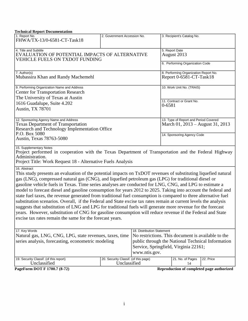
i

Technical Report Documentation 1. Report No.

FHWA/TX-13/0-6581-CT-Task18 2. Government Accession No.

3. Recipient's Catalog No.

4. Title and Subtitle

EVALUATION OF POTENTIAL IMPACTS OF ALTERNATIVE VEHICLE FUELS ON TXDOT FUNDING

5. Report Date

August 2013

6. Performing Organization Code

7. Author(s)

Mubassira Khan and Randy Machemehl 8. Performing Organization Report No.

Report 0-6581-CT-Task18

9. Performing Organization Name and Address

Center for Transportation Research

The University of Texas at Austin

1616 Guadalupe, Suite 4.202

Austin, TX 78701

10. Work Unit No. (TRAIS)

11. Contract or Grant No.

0-6581

12. Sponsoring Agency Name and Address

Texas Department of Transportation Research and Technology Implementation Office P.O. Box 5080 Austin, Texas 78763-5080

13. Type of Report and Period Covered

March 01, 2013 – August 31, 2013

14. Sponsoring Agency Code

15. Supplementary Notes

Project performed in cooperation with the Texas Department of Transportation and the Federal Highway Administration. Project Title: Work Request 18 - Alternative Fuels Analysis

16. Abstract

This study presents an evaluation of the potential impacts on TxDOT revenues of substituting liquefied natural

gas (LNG), compressed natural gas (CNG), and liquefied petroleum gas (LPG) for traditional diesel or

gasoline vehicle fuels in Texas. Time series analyses are conducted for LNG, CNG, and LPG to estimate a

model to forecast diesel and gasoline consumption for years 2012 to 2025. Taking into account the federal and

state fuel taxes, the revenue generated from traditional fuel consumption is compared to three alternative fuel

substitution scenarios. Overall, if the Federal and State excise tax rates remain at current levels the analysis

suggests that substitution of LNG and LPG for traditional fuels will generate more revenue for the forecast

years. However, substitution of CNG for gasoline consumption will reduce revenue if the Federal and State

excise tax rates remain the same for the forecast years.

17. Key Words

Natural gas, LNG, CNG, LPG, state revenues, taxes, time

series analysis, forecasting, econometric modeling

18. Distribution Statement

No restrictions. This document is available to the

public through the National Technical Information

Service, Springfield, Virginia 22161;

www.ntis.gov.

19. Security Classif. (of this report)

Unclassified 20. Security Classif. (of this page)

Unclassified 21. No. of Pages

54 22. Price

PageForm DOT F 1700.7 (8-72) Reproduction of completed page authorized

i

EVALUATION OF POTENTIAL IMPACTS OF ALTERNATIVE

VEHICLE FUELS ON TXDOT FUNDING

by

Mubassira Khan

Graduate Research Assistant

The Center for Transportation Research

The University of Texas

and

Randy Machemehl, P.E.

Professor

The Center for Transportation Research

The University of Texas

Project 0-6581-CT-Task18

TxDOT Administration Research: Task 18 (FY13) Alternative Fuels Analysis

Performed in cooperation with the

Texas Department of Transportation

and the

Federal Highway Administration

August 2013

CENTER FOR TRANSPORTATION RESEARCH

The University of Texas at Austin

1616 Guadalupe Street, Suite 4.200

Austin, Texas 78701

ii

DISCLAIMER

The contents of this report reflect the views of the author(s), who are responsible for the facts

and the accuracy of the data presented herein. The contents do not necessarily reflect the official

view or policies of the Federal Highway Administration (FHWA) or the Texas Department of

Transportation (TxDOT). This report does not constitute a standard, specification, or regulation.

ACKNOWLEDGEMENTS

This project was conducted in cooperation with the Texas Department of Transportation. The

authors also acknowledge the valuable contributions of Shannon Crum and Cary Choate for their

input and feedback during the development of this research.

iii

TABLE OF CONTENTS

CHAPTER 1. BACKGROUND 1

CHAPTER 2. LIQUEFIED NATURAL GAS (LNG) 6

1. INTRODUCTION TO LNG 6

2. METHODOLOGY 7

Model Performance Evaluation 8

3. ANALYSIS AND RESULTS 9

Explanatory Variables 9

Data Sources 9

Model Estimation 10

Validation/Model Performance Evaluation 11

Forecasting 12

4. REVENUE CALCULATION 13

5. CONCLUSIONS 16

CHAPTER 3. COMPRESSED NATURAL GAS (CNG) 17

1. INTRODUCTION TO CNG 17


Model Estimation 19

Validation/Model Performance Evaluation 21

Forecasting 23

Revenue Calculation 25

3. CONCLUSION 29

CHAPTER 4. LIQUEFIED PETROLEUM GAS (LPG) 31

1. INTRODUCTION TO LPG 31


Revenue Forecast 34

3. CONCLUSIONS 36

CHAPTER 5. CONCLUSIONS AND RECOMMENDATIONS 38

REFERENCES 41

APPENDIX 45

iv

LIST OF FIGURES

Figure 1. Annual Diesel Consumption Model and Forecast (Trend Stationary Process)…………9

Figure 2. Annual Diesel Consumption Model and Forecast (Time Series Model Including

Exogenous Variables). .................................................................................................................. 13

Figure 3. Annual Diesel Consumption Model and Forecast (First-Order Autoregressive Time

Series Model). ............................................................................................................................... 13 Figure 4. Estimated Average Revenue......................................................................................... 15 Figure 5. Added Revenue from LNG Conversion. ...................................................................... 15 Figure 7. Residual Plot for Time Series Model with Explanatory Variables (Model 2). ........... 22

Figure 8. Residual Plot for First-Order Autoregressive Error Model (Model 3). ........................ 22 Figure 9. Annual Gasoline Consumption Model and Forecast (Trend Stationary Process, Model

1). .................................................................................................................................................. 24 Figure 10. Annual Gasoline Consumption Model and Forecast (Time Series Model including

Exogenous Variables, Model 2). ................................................................................................... 25 Figure 11. Annual Gasoline Consumption Model and Forecast (First-Order Autoregressive Error

Model, Model 3). .......................................................................................................................... 25 Figure 12. Estimated Annual Revenue. ....................................................................................... 27

Figure 13. Forecast Years Annual Revenue Estimates. ............................................................... 28 Figure 14. Total revenue for different state tax on CNG. ............................................................ 28 Figure 15. Differences in revenue for different state tax rates on CNG for year 2015. .............. 29

Figure 16. Estimated Annual Revenue. ...................................................................................... 35 Figure 17. Forecast Years Annual Revenue Estimates. ............................................................... 36

Figure 18. Annual Diesel Consumption Historical Data. ........................................................... 46 Figure 19. Projected Per Capita Income ($)................................................................................. 46 Figure 20. Projected Texas Population. ....................................................................................... 47

Figure 21. Projected Texas GDP. ................................................................................................ 47

Figure 22. Residual Plot for Time Stationary Model (Model 1).................................................. 48 Figure 23. Residual Plot for Time Series Model with Explanatory Variables (Model 2). .......... 48 Figure 24. Residual Plot for First-Order Autoregressive Model (Model 3). ............................... 49

Figure 25. Annual Gasoline Consumption Historical Data. ........................................................ 53 Figure 26. Projected Texas Population. ....................................................................................... 53

Figure 27. Projected Texas GDP. ................................................................................................ 54

v

LIST OF TABLES

Table 1. Trend-Stationary Model Results. .................................................................................... 10 Table 2. Time Series Model Results, Including Explanatory Variables. ..................................... 10 Table 3. First-Order Autoregressive Model Results. .................................................................... 11

Table 4. Tax Rates Used in Revenue Calculation........................................................................ 14 Table 5. Estimated Revenue from LNG Conversion. .................................................................. 16 Table 6. Trend-Stationary Model Results. ................................................................................... 19 Table 7. Time Series Model Results, Including Explanatory Variables. ..................................... 20 Table 8. First-Order Autoregressive Error Model Results. ......................................................... 21

Table 9. Model 1 Performance Measures. ................................................................................... 23 Table 10. Model 2 Performance Measures. ................................................................................. 23 Table 11. Model 3 Performance Measures. ................................................................................. 23 Table 12. Tax Rates Used in Revenue Calculation...................................................................... 26

Table 13. Tax rates used in revenue calculation. ......................................................................... 34 Table 14. Estimated Revenue from LNG Conversion. ................................................................ 36

Table 15. Listing of Texas Diesel Consumption, Per Capita Personal Income and Population

Data (1984–2011). ........................................................................................................................ 45

Table 16. Model 1 Performance Measures .................................................................................. 49 Table 17. Model 2 Performance Measures. ................................................................................. 49 Table 18. Model 3 Performance Measures. ................................................................................. 50

Table 19. Listing of Texas Gasoline Consumption, Population, and GDP Data (1981–2011). .. 51 Table 20. CNG State Tax Rates. .................................................................................................. 52

1

CHAPTER 1. BACKGROUND

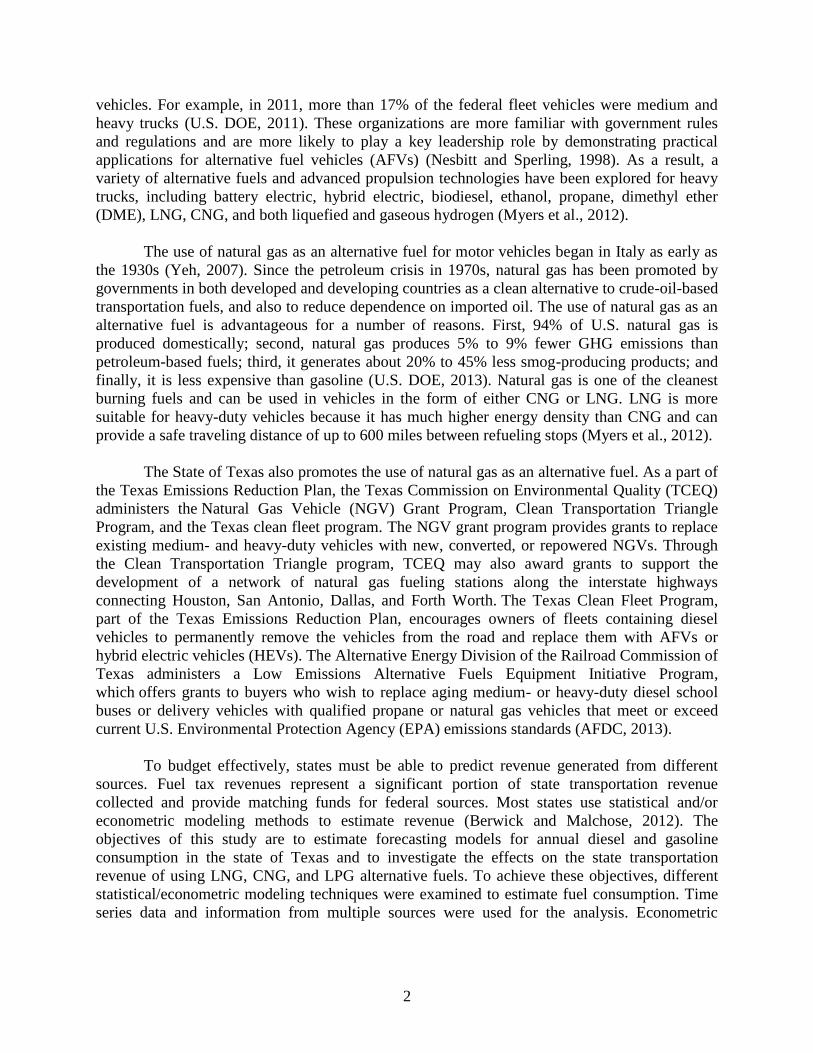
The transportation sector accounts for more than half of world oil consumption (Hirsch et al.,

2005). In the United States, about 90% of the fuel used for on-road vehicular travel is petroleum-

based, which includes gasoline and diesel (Ribeiro et al., 2007). In 2010, the transportation

sector was responsible for 27% of greenhouse gas (GHG) emissions in the U.S.—the second

largest source of GHG emissions, exceeded only by electrical energy generation (EPA, 2010). In

addressing both the transportation sector’s dependence on oil and air quality concerns,

alternative fuel vehicles (AFV) offer opportunities.

Alternative fuels are derived from resources other than crude oil and they usually produce

less pollution than gasoline and diesel. Some alternative fuels are produced domestically. The

Energy Policy Act (EPAct) of 1992 defines alternative fuels to include ethanol (blends of 85% or

more), electricity, biodiesel (B100), compressed natural gas (CNG), liquefied natural gas (LNG),

liquefied petroleum gas (LPG or propane), P-Series fuels, hydrogen, methanol (blends of 85% or

more), and coal-derived liquid fuels (U.S. DOE, 2009). Traditionally, the preferred fuels for

motorized vehicles have been petroleum-based because of their high energy density and low

cost. However, the worldwide increased demand for oil and the perceived unreliability of foreign

oil supplies have resulted in fluctuating and steadily increasing petroleum fuel prices. Studies on

the 1970s energy crisis indicate that the cost to the U.S. economy from a future oil price crisis

could be enormous. These studies estimate the macroeconomic impacts as reducing U.S.

economic activity by an average of over 2% per year for three to four years or more, which

translates into gross national product (GNP) reductions in the range of $600 billion over three

years, up to possibly $3 trillion over fifteen years if the lost economic growth were not

subsequently made up (see NHTSA, 2002; EMF, 1992; Greene and Leiby, 1993). Therefore,

substituting gasoline and diesel with alternative fuels could play a major role in reducing the

vulnerability of the U.S. transportation sector to the disruption and fluctuation of the petroleum

supply and significantly benefit the U.S. economy. The federal government—specifically the

Department of Energy (DOE), the General Services Administration, and the Department of

Agriculture—are involved in efforts to promote the use and expansion of alternative fuels and

the alternative fuel infrastructure.

Vehicle characteristics and movement behavior of freight hauling trucks make them an

attractive market for promoting alternative fuels. The 2007 Commodity Flow Survey reports that

70% of all shipments made via single mode were shipped by truck. Policymakers prefer trucks to

promote the use of alternative fuels for a number of reasons. First, the average annual vehicle

miles driven by trucks are much higher compared to household personal vehicles (FHWA,

2010). In 2010, the average annual vehicle miles traveled (VMT) per passenger vehicle

(including both passenger cars and light-duty trucks) was 11,492 miles. The average VMT for

trucks (all classes) was 26,604 miles (FHWA, 2010). For a class 8 truck (weight ≥ 33,001), the

average annual VMT was 68,907 miles (U.S. DOE, 2012). Therefore, the potential energy and

emissions benefits of alternative fueling are greater per converted truck than per converted

passenger vehicle. Second, while trucks made up only 4.3% of the vehicles on the road in 2010,

they accounted for more than 26% of the fuel consumed in the U.S. (FHWA, 2010). Per-vehicle

fuel consumption and fuel cost are key drivers for adopting new technology for heavy trucks.

Third, government agencies or regulated companies purchase a significant number of fleet

2

vehicles. For example, in 2011, more than 17% of the federal fleet vehicles were medium and

heavy trucks (U.S. DOE, 2011). These organizations are more familiar with government rules

and regulations and are more likely to play a key leadership role by demonstrating practical

applications for alternative fuel vehicles (AFVs) (Nesbitt and Sperling, 1998). As a result, a

variety of alternative fuels and advanced propulsion technologies have been explored for heavy

trucks, including battery electric, hybrid electric, biodiesel, ethanol, propane, dimethyl ether

(DME), LNG, CNG, and both liquefied and gaseous hydrogen (Myers et al., 2012).

The use of natural gas as an alternative fuel for motor vehicles began in Italy as early as

the 1930s (Yeh, 2007). Since the petroleum crisis in 1970s, natural gas has been promoted by

governments in both developed and developing countries as a clean alternative to crude-oil-based

transportation fuels, and also to reduce dependence on imported oil. The use of natural gas as an

alternative fuel is advantageous for a number of reasons. First, 94% of U.S. natural gas is

produced domestically; second, natural gas produces 5% to 9% fewer GHG emissions than

petroleum-based fuels; third, it generates about 20% to 45% less smog-producing products; and

finally, it is less expensive than gasoline (U.S. DOE, 2013). Natural gas is one of the cleanest

burning fuels and can be used in vehicles in the form of either CNG or LNG. LNG is more

suitable for heavy-duty vehicles because it has much higher energy density than CNG and can

provide a safe traveling distance of up to 600 miles between refueling stops (Myers et al., 2012).

The State of Texas also promotes the use of natural gas as an alternative fuel. As a part of

the Texas Emissions Reduction Plan, the Texas Commission on Environmental Quality (TCEQ)

administers the Natural Gas Vehicle (NGV) Grant Program, Clean Transportation Triangle

Program, and the Texas clean fleet program. The NGV grant program provides grants to replace

existing medium- and heavy-duty vehicles with new, converted, or repowered NGVs. Through

the Clean Transportation Triangle program, TCEQ may also award grants to support the

development of a network of natural gas fueling stations along the interstate highways

connecting Houston, San Antonio, Dallas, and Forth Worth. The Texas Clean Fleet Program,

part of the Texas Emissions Reduction Plan, encourages owners of fleets containing diesel

vehicles to permanently remove the vehicles from the road and replace them with AFVs or

hybrid electric vehicles (HEVs). The Alternative Energy Division of the Railroad Commission of

Texas administers a Low Emissions Alternative Fuels Equipment Initiative Program,

which offers grants to buyers who wish to replace aging medium- or heavy-duty diesel school

buses or delivery vehicles with qualified propane or natural gas vehicles that meet or exceed

current U.S. Environmental Protection Agency (EPA) emissions standards (AFDC, 2013).

To budget effectively, states must be able to predict revenue generated from different

sources. Fuel tax revenues represent a significant portion of state transportation revenue

collected and provide matching funds for federal sources. Most states use statistical and/or

econometric modeling methods to estimate revenue (Berwick and Malchose, 2012). The

objectives of this study are to estimate forecasting models for annual diesel and gasoline

consumption in the state of Texas and to investigate the effects on the state transportation

revenue of using LNG, CNG, and LPG alternative fuels. To achieve these objectives, different

statistical/econometric modeling techniques were examined to estimate fuel consumption. Time

series data and information from multiple sources were used for the analysis. Econometric

http://www.propane.tx.gov/Rebates_and_Incentives

3

models were developed to estimate annual diesel consumption, based on historical data from

1981 to 2011 for annual fuel sales, VMT, fuel price, per capita personal income, and population.

Report Summary

This study presents an evaluation of the potential impacts on TxDOT revenues of substituting

liquefied natural gas (LNG), compressed natural gas (CNG) and liquefied petroleum gas (LPG)

for diesel fuel in heavy-duty vehicles in Texas. Time series analysis is conducted to estimate a

model to forecast diesel and gasoline consumption for years 2012 to 2025. Taking into account

the federal and state fuel taxes, the revenue generated from diesel and gasoline consumption is

compared to revenue that could be generated for LNG, CNG and LPG substitution scenarios.

Overall, the result of the analysis suggests that substitution of LNG and LPG for diesel

consumption will generate more revenue if the federal and state excise tax rates remain the same

for the forecast years. Substitution of CNG for gasoline will decrease state revenue unless the

CNG gas tax is raised.

The following points highlight the results:

Regarding LNG substitution for Diesel Fuel

Due to cost of fuel conversion and physical size of LNG on-board vehicle fuel tanks,

trucks rather than passenger cars are the most suitable vehicle type for LNG fueling.

Since the truck fleet is largely fueled by diesel, this report forecasts diesel consumption

through 2025 and then considers the impacts of converting from diesel to LNG at the

rates of 10, 20, and 50%.

Current tax rates for diesel and LNG fuel are $0.44 and $0.269 per liquid gallon,

including both Texas state and federal excise taxes. However, Texas receives

approximately 87.9% of the federal tax collected in Texas for both fuels, yielding the

effective tax rates of $0.4145 and $0.2546 for diesel and LNG, respectively.

LNG provides only about 60% of the energy of an equivalent volume of diesel, meaning

the user must purchase 1.67 gallons of LNG to travel the same distance as on 1 gallon of

diesel.

Because users must buy more LNG to go the same distance, after adjusting for the

fraction of federal tax received by Texas, the effective tax rates are $0.414 per gallon of

diesel and $0.424 per energy equivalent gallon for LNG.

Although the trucking community has some interest in LNG, this interest seems to be

based primarily on LNG prices being less than diesel fuel. Current pump prices at Texas

retail outlets selling LNG fuel are approximately $2.75 per gallon compared to about

$3.90 per gallon for diesel. However, the LNG energy equivalent price (computed by

dividing $2.75 by 0.6) is $4.58 per gallon.

Current federal law (through December 31, 2013) provides a $0.50 per gallon tax rebate

for LNG purchases. This rebate is paid from general revenue, not the Highway Trust

Fund.

4

Regarding CNG Substitution for Gasoline

Light-duty vehicles, including passenger cars and light-duty trucks, are the most suitable

vehicles for CNG fueling because the driving ranges of CNG-fueled vehicles are limited.

CNG has only 25% of the energy density of diesel fuel.

Since the light-duty vehicle fleet is largely fueled by gasoline, this report forecasts gasoline

consumption through 2025 and then considers the impacts of converting from gasoline to

CNG at the rates of 10, 20, and 50%.

The tax rates and consumer “pump” prices are based on “gasoline gallon equivalents”

(GGE) because CNG is sold in a gaseous form—not as a liquid. In other words, CNG is sold

in a quantity containing approximately the same energy as one gallon of gasoline.

The current tax rate for gasoline is $0.384 per liquid gallon and for CNG fuel is $0.333 per

GGE (this figure includes both Texas state and federal excise taxes). However, Texas

receives approximately 83.9% of the federal tax collected in Texas for gasoline and

approximately 93.3% of the federal CNG tax collected in Texas. Applying these

adjustments, the effective tax rates are $0.354 and $0.321 for gasoline and CNG,

respectively.

Given the current effective excise tax rates for gasoline versus CNG, TxDOT will lose

revenue as CNG replaces gasoline as a vehicle fuel. Based upon current federal and state tax

rates and percentages of federal taxes returned to Texas, increasing the current $0.15 per

GGE CNG state tax rate to $0.1836 per GGE will provide equivalent effective tax rates for

gasoline and CNG.

Interest in CNG within the light-duty vehicle community seems to be based primarily on

CNG reducing consumer costs.

o Current pump prices are favorable. Texas retail outlets are selling CNG fuel for $2.10

per GGE compared to about $3.50 per gallon for gasoline. In Texas, the state excise tax

is not collected at the pump, so adding $0.15 per gallon brings the actual price to about

$2.25 per GGE.

o Additionally, current federal law (through December 31, 2013) provides a $0.50 per

GGE Alternative Fuel Excise Tax Credit for CNG purchases. This rebate is paid from

general revenue, not the Highway Trust Fund.

o The cost to convert a currently owned or newly purchased light-duty vehicle to CNG is

approximately $10,000 or more. If an LNG user drives 12,000 miles per year, has an

overall fuel economy of 28 miles per gallon, saves $1.25 per gallon using CNG instead

of gasoline, and receives the $0.50 per GGE federal tax credit, then (ignoring inflation)

almost seven years will be required to amortize the CNG conversion cost.

5

Regarding LPG Substitution for Diesel

The driving range and performance of LPG-fueled vehicles is similar to gasoline fueled

vehicles. Although the primary market for LPG has traditionally been residential heating, it

is a viable fuel for light and medium duty vehicles including passenger cars, as well as,

light-and-medium duty trucks since the energy content of LPG is generally about 73% that

of gasoline or 64% of diesel fuel.

Since the light duty vehicle fleet is largely fueled by gasoline, this report forecasts gasoline

consumption through 2025 and LPG use as 10, 20, or 50 percent conversions from gasoline

to LPG.

Current nominal tax rates for gasoline and LPG fuel are $0.384 and $0.286 per liquid gallon

including both Texas State and federal excise taxes. However, Texas receives approximately

83.9 percent of the federal gasoline tax collected in Texas and approximately 88.4 percent of

the federal LPG tax collected in Texas. Adjusting the nominal rates for the fractions of

federal taxes returned to Texas and adjusting for the fact that LPG contains about 73 percent

of the energy of gasoline per unit volume the effective tax rates are $0.354 and $0.370 for

gasoline and LPG, respectively.

Interest within the light- and medium-duty vehicle community in LPG seems to be based

primarily on LPG reducing consumer costs.

o Current pump prices are slightly favorable. Gulf coast retail outlets are selling LPG

fuel for $2.17 per gallon. In Texas, the State excise tax is not collected at the pump

for LPG so adding $0.15 per gallon brings the actual price to about $2.32 per gallon.

The federal tax credit of $0.50 per gallon of LPG fuel reduces the price per gallon to

$1.82. Taking into account the energy density of LPG fuel the gasoline gallon

equivalent price of LPG fuel is $2.49 compared to about $3.11 per gallon for

gasoline.

o Additionally, the federal tax credit (through 31 December 2013) of $0.50 per gallon

of LPG is paid from general revenue not the Highway Trust Fund.

o Conversion costs for either currently owned or newly purchased light duty vehicles

are not so favorable at approximately $4,000 or more. If one drives 12,000 miles per

year, has overall fuel economy of 28 miles per gallon, saves $0.62 per gallon using

LPG instead of gasoline (this includes the $0.50 per GGE federal tax credit) ignoring

inflation, almost fifteen years will be required to amortize the LPG conversion cost.

6

CHAPTER 2. LIQUEFIED NATURAL GAS (LNG)

1. INTRODUCTION TO LNG

LNG is an odorless, colorless, noncorrosive, and nontoxic fuel. LNG is composed of almost

100% methane derived from natural gas after extraction from underground shale reserves.

During the liquefaction process, oxygen, carbon dioxide, sulfur compounds, and water are

removed, purifying the fuel. As a result, LNG-fueled vehicles can offer significant emissions

benefits compared with diesel-powered vehicles, and can significantly reduce carbon monoxide

and particulate emissions as well as nitrogen oxide emissions (EPA 2002). Moreover, LNG is

domestically produced in the U.S., while diesel is manufactured using oil, of which nearly two-

thirds is imported (AFDC, 2012). Advances in horizontal drilling and fracturing technology that

facilitate the extraction of natural gas have resulted in an abundance of domestic natural gas,

such that its price has decoupled from petroleum (Myers et al., 2012) and is currently

significantly lower than the diesel price (Silverstein, 2013; Sutherland, 2011 ). However, LNG is

a cryogenic fuel that will gradually degrade; as a perishable product in storage, it must be

consumed in a timely manner (Myers et al., 2012). As LNG must be stored at extremely low

temperatures, the tanks required to maintain these temperatures on vehicles are large. On

average, LNG tanks require 70% more volume than diesel tanks for the same energy storage

(TIAX, 2013).

Early research regarding the viability of LNG for heavy trucks was conducted based on a

fleet of LNG-fueled refuse trucks operated in 1997 in Pittsburg, Pennsylvania, by a private

company, Waste Management, Inc. The driver responses regarding the LNG fuel were very

positive, in part because LNG-fueled engines generate less noise than diesel-powered engines.

The use of cleaner fuel also helped the company when bidding on waste hauling contracts in

cities trying to improve air quality (EPA, 2002). Recent research on alternative fuel suggests the

use of LNG as a feasible alternative fuel for long-haul commercial trucks (Myers et al., 2012).

In recent years, oil prices have fluctuated while the price of natural gas has remained

steady and lower in comparison. Increasing diesel prices have motivated trucking companies to

operate trucks that run on natural gas and buy new trucks that are powered by natural gas—even

though LNG-fueled trucks can cost as much as $30,000 more than diesel-fueled trucks (The Wall

Street Journal, 2012). Additionally, LNG gas use is also encouraged by a tax incentive. A tax

credit of $0.50 per gallon is available for LNG users between January 1, 2005, and December 31,

2013 (U.S. DOE). From the trucking company perspective, this tax incentive can be used to

offset higher initial vehicle purchase or conversion costs. Diesel-fueled trucks can be converted

to use LNG through a process available from several vendors; currently approximate costs run

from $10,000 to $18,000 depending on the engine size and desired vehicle range (which affects

the size of the LNG fuel tanks). At least two vendors, EcoDual LLC and Peake Fuel Solutions

LLC, have conversions kits available that allow diesel trucks to run on a mixture of diesel and up

to 85% or 70% natural gas but retain the ability to run on 100% diesel when natural gas fuels are

not available. Due to the current lack of LNG or CNG fueling stations, the dual fuel capability

offered by these kits seems to be very desirable. The Peake kit has only recently been approved

by the EPA and is becoming commercially available during spring 2013.

7

The likelihood of LNG consuming a significant fraction of the diesel motor fuel market

is, of course, dependent upon the market prices of the two competing products. A check of LNG

prices at the pump in the Houston area in mid-March 2013 indicates that the prices were

approximately $2.75 per liquid gallon. Diesel fuel at the same outlets was priced around $3.90

per gallon. While this might appear to be a significant LNG price advantage, if we adjust for the

energy density of the two fuels (dividing the LNG price by 0.60 to reach the energy density of

diesel), the LNG price becomes $4.58 per equivalent gallon. Applying the $0.50 per gallon

federal tax credit, the LNG price becomes $4.08 per gallon—or very close to that of diesel fuel.

(By the way, under current law, the $0.50 per gallon tax credit is being paid from the federal

general fund, not the Highway Trust Fund, so it does not currently affect the transportation

revenue available to Texas.) We can reasonably expect that retail outlets will price LNG near the

price they charge for diesel fuel since it is the competing product and they have little incentive to

reduce their potential profit margins. Wholesale prices for LNG—the prices paid by retail

vendors and very large consumers—are rumored to be approximately half the Houston pump

prices. If that is true, we might expect pump prices to moderate as more vendors enter the market

and more consumers seek LNG fuel.

2. METHODOLOGY

Forecasting plays a key role for state government agencies to predict revenues and estimate cash

flow. A sound forecasting method can help improve future investment planning and maximize

investment returns. Most states employ statistical and/or econometric models to estimate and

forecast fuel consumption. In most cases, observed historical data is used to find the parameters

of a specified relationship that fit the observed data most closely. The parameters obtained using

observations from the past are used to forecast future estimates. In this study we employ time

series analysis to estimate annual diesel consumption model parameters that can be used for

forecasting. A brief description of the model is presented in the following sub-section.

Time Series Analysis

Model Structure. A traditional time series model was used to model annual diesel sales.

Let t be the index for annual time period, is the diesel consumption at time t, is a

corresponding vector of coefficients to be estimated (including a constant), denotes the

sequence of errors or disturbances, denotes the set of all independent

variables in the equation at time t, and further X denotes the collection of all independent

variables in the equation at time t.

The following assumptions are required for the time series model.

Assumptions

1. The time series process follows a model that is linear in parameters.

2. In the sample (and therefore in the underlying time series process), no independent

variable is constant and no independent variable is a perfect linear combination of the

others.

ty

tu

),....,,,( 321 tkttt xxxxtx

tt uy tx

8

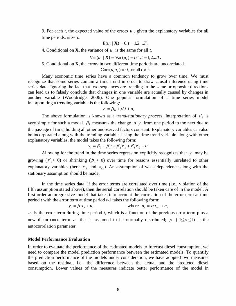
3. For each t, the expected value of the errors , given the explanatory variables for all

time periods, is zero.

4. Conditional on X, the variance of is the same for all t.

5. Conditional on X, the errors in two different time periods are uncorrelated.

Many economic time series have a common tendency to grow over time. We must

recognize that some series contain a time trend in order to draw causal inference using time

series data. Ignoring the fact that two sequences are trending in the same or opposite directions

can lead us to falsely conclude that changes in one variable are actually caused by changes in

another variable (Wooldridge, 2006). One popular formulation of a time series model

incorporating a trending variable is the following:

The above formulation is known as a trend-stationary process. Interpretation of is

very simple for such a model. measures the change in from one period to the next due to

the passage of time, holding all other unobserved factors constant. Explanatory variables can also

be incorporated along with the trending variable. Using the time trend variable along with other

explanatory variables, the model takes the following form:

Allowing for the trend in the time series regression explicitly recognizes that may be

growing ( > 0) or shrinking ( < 0) over time for reasons essentially unrelated to other

explanatory variables (here and ). An assumption of weak dependence along with the

stationary assumption should be made.

In the time series data, if the error terms are correlated over time (i.e., violation of the

fifth assumption stated above), then the serial correlation should be taken care of in the model. A

first-order autoregressive model that takes into account the correlation of the error term at time

period t with the error term at time period t-1 takes the following form:

is the error term during time period t, which is a function of the previous error term plus a

new disturbance term that is assumed to be normally distributed; (-1≤ ≤1) is the

autocorrelation parameter.

Model Performance Evaluation

In order to evaluate the performance of the estimated models to forecast diesel consumption, we

need to compare the model prediction performance between the estimated models. To quantify

the prediction performance of the models under consideration, we have adopted two measures

based on the residual, i.e., the difference between the actual and the predicted diesel

consumption. Lower values of the measures indicate better performance of the model in

tu

.,...2,1,0)|(E Ttut X

tu

.,...2,1,)(Var)|(Var 2 Ttuu tt X

stuu st allfor ,0)(Corr

tt uty 10

1

1 ty

tttt uxxty 231210

ty

1 1

1tx 2tx

ttttt uu uy 1 wheretx

tu

t

9

forecasting future share prices. The first measure is the sum of the absolute residual for the two-

year time period, which can be expressed as

The next performance measure is the sum of the square of the residual for the forecasted

two years and can be expressed as

3. ANALYSIS AND RESULTS

To estimate the diesel consumption model, we reviewed various combinations of independent

variables and two different functional forms of time series analysis to arrive at the best

alternative annual forecast model. The study examines data issues, model specifications, critical

assumptions, and forecast performance. Two different forms of dependent variables are

analyzed. The first one is the diesel consumption in million gallons and the second one is the loge

of diesel consumption in gallons. The second model gives a better R-squared value for all the

models and is presented in the report. Time series data for the dependent and explanatory

variables are collected from 1984 to 2011. The diesel consumption model is estimated using data

from 1984 to 2009. Two years of data (year 2010 and 2011) are used to validate the model

results and to evaluate model performance. The data used in the analysis is shown in the

Appendix A.

Explanatory Variables

Different explanatory variables are considered for estimating the diesel consumption model. The

fuel demand (gasoline and/or diesel) models used by other state DOTs and state agencies are

reviewed to get a clear picture about the state of practice. Explanatory variables used to estimate

the fuel consumption model include fuel efficiency, real per-capita personal income, population,

population growth, wages, salary growth, VMT, real gasoline price, real disposable income,

vehicle fleet size, and employment data (Berwick and Malchose, 2012, WSDOT, 2010). Fuel

price and VMT variables appear very tempting to use as explanatory variables for estimating fuel

demand. However, estimating future gas prices and VMT are very difficult tasks. Moreover,

these variables are more likely to be endogenous to the response variable diesel consumption.

The variables tested to obtain the final model specification include population, per capita

personal income, and gross domestic product (GDP).

Data Sources

Multiple sources of data and information are used to support the analyses and conclusions in this

report. The dependent variable of this study is the annual diesel sales to on-highway consumers

in Texas. The diesel consumption data from 1984 to 2011 is collected from the U.S. Energy

Information Administration (EIA). Yearly population data is obtained from the Texas

Department of State Health Services. Per capita personal income and GDP data are collected

from the Bureau of Economic Analysis (BEA). Federal and state tax data are collected from the

FHWA website to estimate revenue generated from diesel consumption.

The estimated model specification and results are presented in the following section.

2011

2010 , ||T

t Forecasttt yy

2011

2010

2

, )(T

t Forecasttt yy

10

Model Estimation

Model 1: Trend Stationary Model

The first model we estimate is a trend-stationary model where time is the only explanatory

variable used in the analysis. We assume there is no serial correlation between the error terms.

The parameter estimates of the trend-stationary model are presented in Table 1.

Table 1. Trend-Stationary Model Results.

Dependent Variable: loge(Diesel Consumption in Gallons)

Variable Parameter Estimate t-Value Pr > |t|

Intercept -80.143 -14.98 <0.0001

Year 0.051 19.01 <0.0001

R-square value 0.938

The coefficient of the trend variable (year) is statistically significant (p-value <0.0001). The year

variable can be interpreted as the average per year growth rate in diesel consumption. That

means the diesel consumption grows about 5.1% per year on average, holding all other factors

fixed. The incorporation of time as an independent variable to explain the variation in diesel

consumption performs very well with an R-square value of 0.9377 and root mean square error of

0.10244.

Model 2: Time Series Model with Explanatory Variables

We incorporated three exogenous variables in addition to the trend variable in the regression

equation. The variables considered are loge(population), loge(per capita personal income), and

loge(GDP). The parameter estimate of the ln (GDP) variable is found to have a negative sign,

which is very counterintuitive. The variable is also not statistically significant at a 0.05

significance level and was removed from the model. The model specification with statistically

significant parameter estimates is presented in Table 2.

Table 2. Time Series Model Results, Including Explanatory Variables.

Dependent Variable: loge(Diesel Consumption in gallons)

Variable Parameter

Estimate

t-Value Pr > |t|

Intercept 209.034 6.49 <0.0001

Year -0.109 6.09 <0.0001

ln (Per Capita Personal Income $) 1.599 5.18 <0.0001

ln (Population in millions) 4.865 7.91 <0.0001


After incorporating exogenous variables, the model is able to explain most of the

timewise variation in diesel consumption. The R-squared value of this model is 0.988 and the

root mean square is 0.0479. As expected, per capita personal income and population are

positively correlated with the diesel consumption. The estimated parameter for the ln(per capita

personal income) variable is 1.599, which in a log-log model is also the income elasticity for

11

diesel consumption. The estimated parameter of the ln(population) variable is 4.865, which in the

log-log model is the population elasticity for diesel consumption. After accommodating the

explanatory variables in the model, the trend variable exhibits a shrinking nature. That means the

diesel consumption shrinks about 10.9% per year on average, holding all other factors fixed.

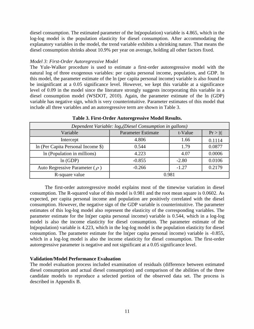
Model 3: First-Order Autoregressive Model

The Yule-Walker procedure is used to estimate a first-order autoregressive model with the

natural log of three exogenous variables: per capita personal income, population, and GDP. In

this model, the parameter estimate of the ln (per capita personal income) variable is also found to

be insignificant at a 0.05 significance level. However, we kept this variable at a significance

level of 0.09 in the model since the literature strongly suggests incorporating this variable in a

diesel consumption model (WSDOT, 2010). Again, the parameter estimate of the ln (GDP)

variable has negative sign, which is very counterintuitive. Parameter estimates of this model that

include all three variables and an autoregressive term are shown in Table 3.

Table 3. First-Order Autoregressive Model Results.

Dependent Variable: loge(Diesel Consumption in gallons)


Intercept 4.806 1.66 0.1114

ln (Per Capita Personal Income $) 0.544 1.79 0.0877

ln (Population in millions) 4.223 4.07 0.0006

ln (GDP) -0.855 -2.80 0.0106

Auto Regressive Parameter ( ) -0.266 -1.27 0.2179


The first-order autoregressive model explains most of the timewise variation in diesel

consumption. The R-squared value of this model is 0.981 and the root mean square is 0.0602. As

expected, per capita personal income and population are positively correlated with the diesel

consumption. However, the negative sign of the GDP variable is counterintuitive. The parameter

estimates of this log-log model also represent the elasticity of the corresponding variables. The

parameter estimate for the ln(per capita personal income) variable is 0.544, which in a log-log

model is also the income elasticity for diesel consumption. The parameter estimate of the

ln(population) variable is 4.223, which in the log-log model is the population elasticity for diesel

consumption. The parameter estimate for the ln(per capita personal income) variable is -0.855,

which in a log-log model is also the income elasticity for diesel consumption. The first-order

autoregressive parameter is negative and not significant at a 0.05 significance level.

Validation/Model Performance Evaluation

The model evaluation process included examination of residuals (difference between estimated

diesel consumption and actual diesel consumption) and comparison of the abilities of the three

candidate models to reproduce a selected portion of the observed data set. The process is

described in Appendix B.

12

The sum of the absolute residuals for the two-year model-testing period is much lower for

the second model compared to the first model. The sum of the squares of the residuals for the

forecasted two years is also smaller for Model 2 compared to Model 1 and Model 3. Both of the

measures show that Model 2 (the model with explanatory variables) performs better in

forecasting diesel consumption compared to the other two models.

Forecasting

Using the estimated parameters for the trend stationary model, the diesel consumption is

forecasted for year 2012 to 2025. For the second and third models, the population and the per

capita personal income variables must be estimated using separate models. We use a time

stationary model to estimate and consequently forecast those exogenous variables. For

population, a linear time trend model gives the best model fit. For per capita personal income, a

quadratic time trend model gives the best fit. For GDP, an exponential time trend model gives

the best model fit. Figures 1, 2, and 3 show the diesel consumption model for the estimation

years (labeled 1 in the circle), validation years (labeled 2 in the circle), and forecast year (labeled

3 in the circle) for the three models under consideration. The first model seems to over-estimate

the diesel consumption, especially during the periods of economic recession. The second model

and third models follow the actual diesel consumption data for the estimation and validation

periods very well and therefore are more likely to forecast the diesel consumption better than the

trend stationary model. However, the second model is preferred for the revenue estimation based

on the model performance measures, the intuitive parameter estimates, and the R-squared

statistic. Since statistical models are simplified representations of reality based upon observed

data, economic shocks of recession or spiking oil/fuel prices may render usually reliable

forecasts worthless. Therefore, the expected variation of the diesel consumptions are calculated

for all the models at 95% confidence and shown in the figures with small dashed lines for the

forecast periods.

Figure 1. Annual Diesel Consumption Model and Forecast (Trend Stationary Process).

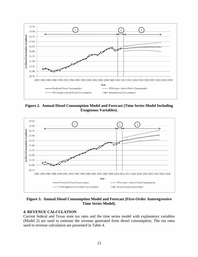
13

Figure 2. Annual Diesel Consumption Model and Forecast (Time Series Model Including

Exogenous Variables).

Figure 3. Annual Diesel Consumption Model and Forecast (First-Order Autoregressive

Time Series Model).

4. REVENUE CALCULATION

Current federal and Texas state tax rates and the time series model with explanatory variables

(Model 2) are used to estimate the revenue generated from diesel consumption. The tax rates

used in revenue calculation are presented in Table 4.

14

Table 4. Tax Rates Used in Revenue Calculation.

Texas and Federal Motor Fuel Excise Taxes

Current Nominal Rates

Diesel LNG

$/gallon $/gallon

Federal 0.244 0.119

State 0.2 0.15

Adjusting for Taxes Received by Texas

[Texas receives 87.9% of federal tax.]

Federal 0.2145 0.1046

State 0.2 0.15

Adjusting for Energy Equivalent Volumes

[LNG contains 60% of the energy per diesel gallon]

Federal 0.2145 0.1743

State 0.2 0.25

Effective Texas Rate Per Liquid Gallon

Total $/gallon 0.4145 0.4243

Table 4 shows that the current nominal excise tax rates are adjusted to account for the

87.9% of federal taxes that actually return to Texas. Because diesel and LNG excise taxes are

based upon liquid gallons, the LNG rate must be adjusted to account for the fact that LNG

contains approximately 60% of the energy in a gallon of diesel. Therefore, roughly speaking, a

vehicle will use 1.667 gallons of LNG to travel the same distance as it could travel on 1 gallon of

diesel. Therefore, the effective tax rates show that almost 1¢ more tax would be collected for

each diesel equivalent gallon of LNG compared to each gallon of diesel fuel.

Based on the estimated diesel consumption and the revenue generated from diesel

consumption, we estimate the revenue for three scenarios where 10%, 20%, and 50% of diesel

consumption would be replaced by LNG consumption. The revenue calculation takes into

account the diesel gallon equivalents (DGE) energy of LNG fuel and the current state and federal

tax rates. The revenue calculation assumes that Texas receives about $0.879 per dollar of

collected federal tax (FHWA, 2010). Inflation rates are not considered in the revenue calculation.

In this study, we assume the tax rates will remain the same for the forecast periods. We also

assume the price of LNG will be competitive with the diesel price. Figure 4 shows the estimated

average revenue for four scenarios from 1984 to 2025.

15

Figure 4. Estimated Average Revenue.

Figure 5 shows the revenue comparison only for the forecast years. The forecast shows

the LNG conversion results in an increase in Texas state revenues. The magnitude of increased

revenue increases as more LNG replaces diesel consumption. The added benefit arises because

1.67 gallons of LNG are required to get the same energy as 1 gallon of diesel.

Figure 5. Added Revenue from LNG Conversion.

The added revenue generated after conversion is calculated for all three scenarios and

presented in Table 5. The LNG conversion can potentially increase the revenues more than $4

million if the LNG substitutes for 10% of diesel consumption in 2013. For the same year, a 20%

substitution yields added revenue of slightly more than $8 million and a 50% substitution results

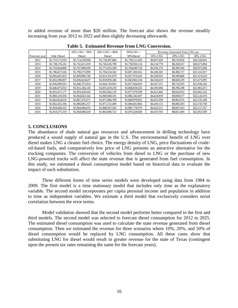
16

in added revenue of more than $20 million. The forecast also shows the revenue steadily

increasing from year 2012 to 2022 and then slightly decreasing afterwards.

Table 5. Estimated Revenue from LNG Conversion.

5. CONCLUSIONS

The abundance of shale natural gas resources and advancement in drilling technology have

produced a sound supply of natural gas in the U.S. The environmental benefit of LNG over

diesel makes LNG a cleaner fuel choice. The energy density of LNG, price fluctuations of crude-

oil-based fuels, and comparatively low price of LNG presents an attractive alternative for the

trucking companies. The conversion of vehicles from diesel to LNG or the purchase of new

LNG-powered trucks will affect the state revenue that is generated from fuel consumption. In

this study, we estimated a diesel consumption model based on historical data to evaluate the

impact of such substitution.

Three different forms of time series models were developed using data from 1984 to

2009. The first model is a time stationary model that includes only time as the explanatory

variable. The second model incorporates per capita personal income and population in addition

to time as independent variables. We estimate a third model that exclusively considers serial

correlation between the error terms.

Model validation showed that the second model performs better compared to the first and

third models. The second model was selected to forecast diesel consumption for 2012 to 2025.

The estimated diesel consumption was used to calculate the state revenue generated from diesel

consumption. Then we estimated the revenue for three scenarios where 10%, 20%, and 50% of

diesel consumption would be replaced by LNG consumption. All these cases show that

substituting LNG for diesel would result in greater revenue for the state of Texas (contingent

upon the present tax rates remaining the same for the forecast years).

10% LNG 20% LNG 50% LNG

2012 $1,710,172,010 $1,714,239,938 $1,718,307,866 $1,730,511,650 $4,067,928 $8,135,856 $20,339,641

2013 $1,738,276,241 $1,742,411,019 $1,746,545,798 $1,758,950,134 $4,134,779 $8,269,557 $20,673,894

2014 $1,763,664,869 $1,767,860,039 $1,772,055,208 $1,784,640,718 $4,195,170 $8,390,340 $20,975,849

2015 $1,786,027,636 $1,790,275,999 $1,794,524,362 $1,807,269,452 $4,248,363 $8,496,727 $21,241,817

2016 $1,805,601,823 $1,809,896,746 $1,814,191,670 $1,827,076,442 $4,294,924 $8,589,848 $21,474,619

2017 $1,822,290,007 $1,826,624,627 $1,830,959,246 $1,843,963,104 $4,334,619 $8,669,239 $21,673,097

2018 $1,836,008,563 $1,840,375,814 $1,844,743,065 $1,857,844,819 $4,367,251 $8,734,503 $21,836,256

2019 $1,846,873,032 $1,851,266,126 $1,855,659,220 $1,868,838,503 $4,393,094 $8,786,188 $21,965,471

2020 $1,855,017,177 $1,859,429,643 $1,863,842,110 $1,877,079,509 $4,412,466 $8,824,933 $22,062,332

2021 $1,860,218,504 $1,864,643,342 $1,869,068,181 $1,882,342,697 $4,424,839 $8,849,677 $22,124,193

2022 $1,862,824,633 $1,867,255,671 $1,871,686,709 $1,884,979,822 $4,431,038 $8,862,076 $22,155,189

2023 $1,862,452,106 $1,866,882,257 $1,871,312,409 $1,884,602,864 $4,430,152 $8,860,303 $22,150,758

2024 $1,859,660,522 $1,864,084,033 $1,868,507,545 $1,881,778,079 $4,423,511 $8,847,023 $22,117,557

2025 $1,854,275,319 $1,858,686,020 $1,863,096,722 $1,876,328,828 $4,410,702 $8,821,404 $22,053,509

Revenue Generated from LNG use

Forecast year Only Diesel

10% LNG + 90%

Diesel

20% LNG + 80%

Diesel

50%LNG +

50%Diesel

17

CHAPTER 3. COMPRESSED NATURAL GAS (CNG)

1. INTRODUCTION TO CNG

Compressed natural gas (CNG) is an alternative fuel derived from natural gas and contains about

95% methane. CNG has become a viable alternative fuel in many countries around the globe in

response to higher gasoline prices and concerns over the environmental impact of petroleum

consumption for transportation. The U.S. Department of Energy (U.S. DOE) reports that CNG

vehicles produce 60% to 90% less smog-producing pollutants and reduce greenhouse gas

emissions by 30% to 40%. In the United States, the price of CNG is less volatile compared with

gasoline because 94% of U.S. natural gas is produced domestically (U.S. DOE). In 2011, about

45% of the petroleum consumed was imported from foreign countries (U.S. EIA). The U.S.

Congress strongly supports reducing petroleum use and has passed laws to provide incentives for

natural gas users.

The State of Texas also promotes the use of CNG as an alternative to gasoline. As a part

of the Texas Emissions Reduction Plan, the Texas Commission on Environmental Quality

(TCEQ) administers the Clean Transportation Triangle Program, which awards grants to support

the development of a network of natural gas fueling stations along the interstate highways

connecting Houston, San Antonio, Dallas, and Forth Worth (U.S. DOE). The Texas Gas Service

Conservation Program offers commercial and residential customers in the Austin and Sunset

Valley area a $2,000 rebate for the purchase of a natural gas vehicle or $3,000 for conversion of

a gasoline-powered vehicle to operate on natural gas, and a $1,000 rebate for the purchase of a

natural gas forklift. The program also offers a $2,000 incentive for the installation of a vehicle-

refueling unit (Texas gas service). CNG gas use is further encouraged by a tax incentive. A tax

credit of $0.50 per gasoline gallon equivalent (GGE) is available for CNG users between January

1, 2005, and December 31, 2013 (U.S. DOE).

CNG vehicles may be safer than traditional vehicles for a number of reasons. The

cylinders that hold the compress natural gas are significantly stronger than gasoline tanks,

making them less likely to ignite after a collision. They have withstood impact and bonfire

testing and meet U.S. Department of Transportation safety standards. Additionally, natural gas is

lighter than air and will dissipate upward rapidly in the unlikely event of a leak (Bakar, 2008;

Texas Gas Service). The long term engine performance of CNG-powered vehicles may also be

better compared with the performance of gasoline-powered vehicles because natural gas does not

produce sludge, acids, and residue, as gasoline does (CNG California).

In the U.S., the price of CNG fuel has remained steady and significantly lower than

gasoline. However, the purchase prices for new CNG-powered vehicles are currently higher

compared with those of gasoline-powered vehicles, although the fuel cost savings of CNG

vehicles can make up the incremental cost over the life of CNG vehicles (Yacobucci, 2011).

Honda manufactures dedicated CNG-powered sedans that are comparable to its gasoline-

powered sedans. The purchase price difference between a conventional Honda Civic EX and a

dedicated CNG-powered Honda Civic GX is roughly $6,000. Gasoline-fueled vehicles can be

converted to use CNG through conversion processes that currently cost approximately $10,000

18

to $18,000 and include the retrofit system, fuel tanks and related tubing/brackets, and installation

(NGV America, 2012).

The likelihood of CNG consuming a significant fraction of the gasoline motor fuel

market is, of course, dependent upon the market prices of the two competing products. A check

on CNG prices at the pump in the Austin area in early April 2013 indicates that the prices were

approximately $2.10 per GGE plus $0.15 state fuel tax. (In Texas, CNG users buy an annual

prepaid tax label based on vehicle weight and miles traveled; this label’s cost is based on $0.15

per GGE state tax). Gasoline fuel at the same time was priced around $3.50 per gallon. Applying

the $0.50 per gallon federal tax credit, the CNG price becomes $1.75 per gallon, which is half

the gasoline price. As already mentioned, under current law, the $0.50 per gallon tax credit is

being paid from the federal general fund, not the Highway Trust Fund, so it does not currently

affect the transportation revenue available to Texas. Assuming the average retail price of

gasoline remains between $1 to $1.75 per gallon greater than CNG, the annual fuel cost savings

of a vehicle using CNG with energy efficiency of 28 miles per gallon and usage of 12,000 miles

per year would be roughly $429 to $750 (U.S. DOE).

Although CNG-fueled vehicles have been in the U.S. market for a long time, their

number is quite small compared to gasoline-fueled vehicles. In 2009, the U.S. had about 114,270

CNG vehicles and 69,018 of them (slightly more than 60%) were light-duty vehicles (U.S. EIA,

2011). This compares with roughly 240 million conventional (mostly gasoline) light-duty

vehicles (Davis et al., 2011). Currently, 574 public CNG stations in the U.S. compete with more

than 120,000 retail gasoline stations (U.S. DOE, Statistics Brain). The market share of CNG

vehicles is not significant because of the higher price of new CNG vehicles, conversion cost,

concerns about vehicle performance, and limited fuel infrastructure (Yacobucci, 2011).

However, the abundance of natural gas in the U.S., the volatile price of gasoline, substantial

price differences between CNG and gasoline, automobile manufacturer interest in CNG light-

duty vehicles, federal and state incentives for CNG infrastructure, and observed environmental

benefits are likely to increase the market share of CNG vehicles. Thus, evaluating the potential

impact on the state economy is crucial.


Because CNG energy density is roughly 25% compared to gasoline, CNG-fueled vehicles need

large on-board storage tanks but still have limited mileage ranges. Range is a significant issue for

heavy-duty long-haul trucks, but it is much less important for light-duty passenger cars and

trucks. Therefore, CNG is generally considered primarily as an alternative fuel for light-duty

gasoline-powered vehicles. If CNG primarily competes with gasoline in the vehicle fuel market,

estimates of its market intrusion might be related to the overall gasoline fuel market.

A gasoline fuel usage prediction model for Texas was developed. To estimate the

gasoline consumption model, combinations of independent variables and three different

functional forms of time series analysis were examined to arrive at the best alternative annual

forecast model. Data issues, model specifications, critical assumptions, and forecast performance

are described. Two different forms of dependent variables were considered: gasoline

consumption in millions of gallons and the loge of gasoline consumption in gallons. The second

model gives a better R-squared value for all the models considered. Time series data for the

19

dependent and explanatory variables were collected from 1981 to 2011. The gasoline

consumption model is estimated using data from 1981 to 2009. Two years of data (2010 and

2011) are used to validate the model results and to evaluate model performance. Appendix C

provides the data used in the analysis.


The gasoline consumption model development process included a review of the fuel demand

(gasoline and/or diesel) models used by other state DOTs and agencies to get a clear picture of

the state of practice. Explanatory variables were considered to estimate the fuel consumption

model include fuel efficiency, real per-capita personal income, population, population growth,

wages, salary growth, vehicle miles traveled (VMT), real gasoline price, real disposable income,

vehicle fleet size, and employment data (Berwick and Malchose, 2012, WSDOT, 2010). Fuel

price and VMT variables are excluded in order to avoid the complexity of their estimation for

future periods. Moreover, these variables are more likely to be endogenous to the response

variable for gasoline consumption. The variables tested to obtain the final model specification

include population, per capita personal income, and gross domestic product (GDP).

Data Sources


report. The dependent variable of this study is the annual gasoline sales to on-highway

consumers in Texas. The gasoline consumption data from year 1981 to 2011 is collected from

the U.S. Energy Information Administration (EIA). Yearly population data is obtained from the

Texas Department of State Health Services. Per capita personal income and GDP data are

collected from the Bureau of Economic Analysis (BEA). Federal and state tax data are collected

from the FHWA website to estimate revenue generated from gasoline consumption.The

estimated model specification and results are presented in the following section.

Model Estimation

Model 1: Trend Stationary Model

The first model we estimate is a trend-stationary model where time is the only explanatory

variable used in the analysis. We assume there is no serial correlation between the error terms.

The parameter estimates of the trend-stationary model are presented in Table 6.

Table 6. Trend-Stationary Model Results.

Dependent Variable: loge(Gasoline Consumption in Gallons)


Intercept -10.6845 -5.59 <0.0001

Year 0.0169 17.60 <0.0001


The coefficient of the trend variable (year) is statistically significant (p-value <0.0001).

The year variable can be interpreted as the average per year growth rate in gasoline consumption.

That means the gasoline consumption grows about 1.7% per year on average, holding all other

factors fixed. The incorporation of time as an independent variable to explain the variation in

20

gasoline consumption performs very well with an R-squared value of 0.9198 and root mean

square error of 0.04318.

Model 2: Time Series Model with Explanatory Variables

We incorporated three exogenous variables in addition to the trend variable in the regression

equation. The variables considered are loge(population), loge(per capita personal income), and

loge(GDP). The per capita personal income variable was not significant and was removed from

the model. The parameter estimates of ln(GDP) and ln(Population) are positive as expected.

Although the GDP variable is not significant at a 0.05 level, we kept it as a proxy of economic

growth over time. The model specification is presented in Table 7.

Table 7. Time Series Model Results, Including Explanatory Variables.

Dependent Variable: loge(Gasoline Consumption in gallons)

Variable Parameter

Estimate t-Value Pr > |t|

Intercept 71.0300 6.84 <0.0001

Year -0.0281 -4.86 <0.0001

ln (GDP in million $) 0.1751 1.73 0.0963



After incorporating exogenous variables, the model is able to explain most of the

timewise variation in gasoline consumption. The R-squared value of this model is 0.9808 and the

root mean square is 0.02199. As expected, GDP and population are positively correlated with

gasoline consumption. The estimated parameter for the ln (GDP in million $) variable is 0.1751,

which in a log-log model is also the GDP elasticity for gasoline consumption. Similarly, the

estimated parameter of the ln(population) variable is 1.9268 and in the log-log model is the

population elasticity for gasoline consumption. After accommodating the explanatory variables

in the model, the trend variable exhibits a shrinking nature. That means the gasoline consumption

shrinks about 2.81% per year on average, holding all other factors fixed.

Model 3: First-Order Autoregressive Error Model

The Yule-Walker procedure is used to estimate a first-order autoregressive error model with the

natural log of three exogenous variables: per capita personal income, population, and GDP. In

this model, the population and the auto regressive parameters are found to be statistically

significant at a 0.05 level.

21

Table 8. First-Order Autoregressive Error Model Results.

Dependent Variable: loge(Gasoline Consumption in gallons)


Intercept 20.2627 103.04 <0.0001


Auto Regressive Parameter ( ) -0.6631 -4.52 <0.0001


The first-order autoregressive model explains most of the timewise variation in gasoline

consumption. The R-squared value of this model is 0.9793 and the root mean square is 0.02235.

As expected, population is positively correlated with the gasoline consumption. However, the

GDP variable is found statistically not significant for the first-order auto-regressive error model.

The parameter estimates of this log-log model also represent the elasticities of the corresponding

variables. The parameter estimate of the ln(population) variable is 0.9190, which in the log-log

model is the population elasticity for gasoline consumption. The first-order autoregressive

parameter is negative and significant at the 0.05 significance level.

Validation/Model Performance Evaluation

We first plot the residuals (difference between the estimated gasoline consumption and the actual

gasoline consumption) of the estimated models to visually examine the residuals’ distribution.

The residual plot for the first model (Figure 6) shows that the residuals of the adjacent periods

have the same sign and also exhibit stickiness between the adjacent periods, indicating the

presence of serial correlation between the error terms of this model. On the other hand, the

residual distribution for Model 2 and Model 3 (Figures 7 and 8) show a fairly random scatter plot

around zero. Very few adjacent residuals are observed to have similar values and display less

stickiness compared to the first model, indicating that the explanatory variables remove most of

the serial correlation. The magnitudes of the residuals are also smaller for both Model 2 and

Model 3 compared to the first model’s residuals.

Figure 6. Residual Plot for Trend Stationary Model (Model 1).

22

Figure 7. Residual Plot for Time Series Model with Explanatory Variables (Model 2).

Figure 8. Residual Plot for First-Order Autoregressive Error Model (Model 3).

The estimated coefficients for the models are used to forecast the gasoline consumption

for year 2010 and 2011. The forecasted values are compared with the actual gasoline

consumption data to calculate the performance measures. The calculated performance measures

for the models are presented in Tables 9-11.

23

Table 9. Model 1 Performance Measures.

Model 1: Trend-Stationary Model

ln (Gasoline Consumption)

∑

∑

Forecasted Actual

23.2208 23.2217 0.000905008 0.00000819

23.2377 23.1988 0.038903329 0.00151347

0.039808337 0.00151428


Model 2: Time Series Model with Exogenous Variable

ln (Gasoline Consumption) ∑

∑

Forecasted Actual

23.2329 23.2217 0.011195 0.000125

23.2568 23.1988 0.058003 0.003364

0.069198 0.003490


Model 3: First-Order Autoregressive Time Series Model

ln (Gasoline Consumption)

∑

∑

Forecasted Actual

23.2224 23.2217 0.000695 0.0000048

23.2442 23.1988 0.045403 0.002061

0.046098 0.002062

The sum of the absolute residuals for the two-year model-testing period is the lowest for

the first model. The sum of the squares of the residuals for the forecasted two-year period is also

smaller for Model 1 compared to Model 2 and Model 3. However, serial autocorrelation is more

likely to be present in the first model compared to the other models. Moreover, a two-year time

period provides a small number of observations for validating the models. However, the sum of

the absolute residuals and the sum of the squares of the residuals for the two-year validation

periods show a better performance of Model 3 compared to Model 2.

Forecasting

Using the estimated parameters for the trend stationary model and the time series model with

exogenous variables, gasoline consumption is forecasted for years 2012 to 2025. For the second

and third models, the population and GDP variables must be estimated using separate models.

We use a trend stationary model to estimate and consequently forecast those exogenous

variables. For population and also for GDP, the exponential trend stationary model gives the best

model fits. Figures 9, 10, and 11 show the gasoline consumption model for the estimation years

(labeled 1 in the circle), validation years (labeled 2 in the circle), and forecast years (labeled 3 in

the circle) for the three models under consideration. The first model seems to over-estimate

24

gasoline consumption, especially during the periods of economic recession. The second and third

models follow the actual gasoline consumption data for the estimation periods very well, but the

third model performs better for the validation periods and therefore is more likely to forecast

future gasoline consumption better than Model 1 or Model 2. Therefore, the third model is

preferred for revenue estimation based on the model performance measures, the intuitive

parameter estimates, and a good R-squared statistic. Since statistical models are simplified

representations of reality using observed data, economic shocks of recession or spiking oil/fuel

prices may render usually reliable forecasts worthless. The expected variations of gasoline

consumption are calculated for all the models at a 95% confidence level and are shown in the

figure as small dotted line bands about the model forecast.

Figure 9. Annual Gasoline Consumption Model and Forecast (Trend Stationary Process,

Model 1).

25

Figure 10. Annual Gasoline Consumption Model and Forecast (Time Series Model

including Exogenous Variables, Model 2).

Figure 11. Annual Gasoline Consumption Model and Forecast (First-Order

Autoregressive Error Model, Model 3).

Revenue Calculation

The models use current federal and Texas state tax rates and the time series model with

explanatory variables (Model 3) to estimate the revenue generated from gasoline consumption.

The tax rates used in revenue calculation are presented in Table 12.

26

Table 12. Tax Rates Used in Revenue Calculation.



Gasoline CNG

$/gallon $/GGE

Federal 0.184 0.183

State 0.200 0.150


Texas receives 83.9% of

federal tax for gasoline.

Texas receives 93.3%

of federal tax for CNG.

Federal 0.154 0.171

State 0.200 0.150

Effective Texas Rate Per Gallon

Total $/gallon 0.354 0.321

Table 12 shows that the current nominal excise tax rates are adjusted to account for the

83.9% of federal tax for gasoline and 93.3% of federal tax for CNG that is actually returned to

Texas. The effective tax rates show that almost 3.36¢ more tax would be collected for each

gallon of gasoline compared to each GGE of CNG fuel. Additionally, although current federal

law (through December 31, 2013) provides a $0.50 per GGE Alternative Fuel Excise Tax Credit

for CNG purchases, this rebate is paid from general revenue, not the Highway Trust Fund.

Therefore, the Alternative Fuel Excise Tax Credit for CNG is excluded from the transportation

revenue calculations.

Based on the estimated gasoline consumption and the revenue generated from gasoline

consumption, we estimate the revenue for three scenarios where 10%, 20%, and 50% of gasoline

consumption would be replaced by CNG consumption. The revenue calculation takes into

account the current state and federal tax rates. The revenue calculation for Texas assumes that

Texas receives about $0.839 per dollar of collected federal tax from gasoline consumption and

$0.933 per dollar of collected federal tax from CNG consumption. Inflation rates are not

considered in the revenue calculation. In this study, we assume the tax rates will remain the same

for the forecast periods. Figure 12 shows the estimated average revenue for four scenarios from

1981 to 2025.

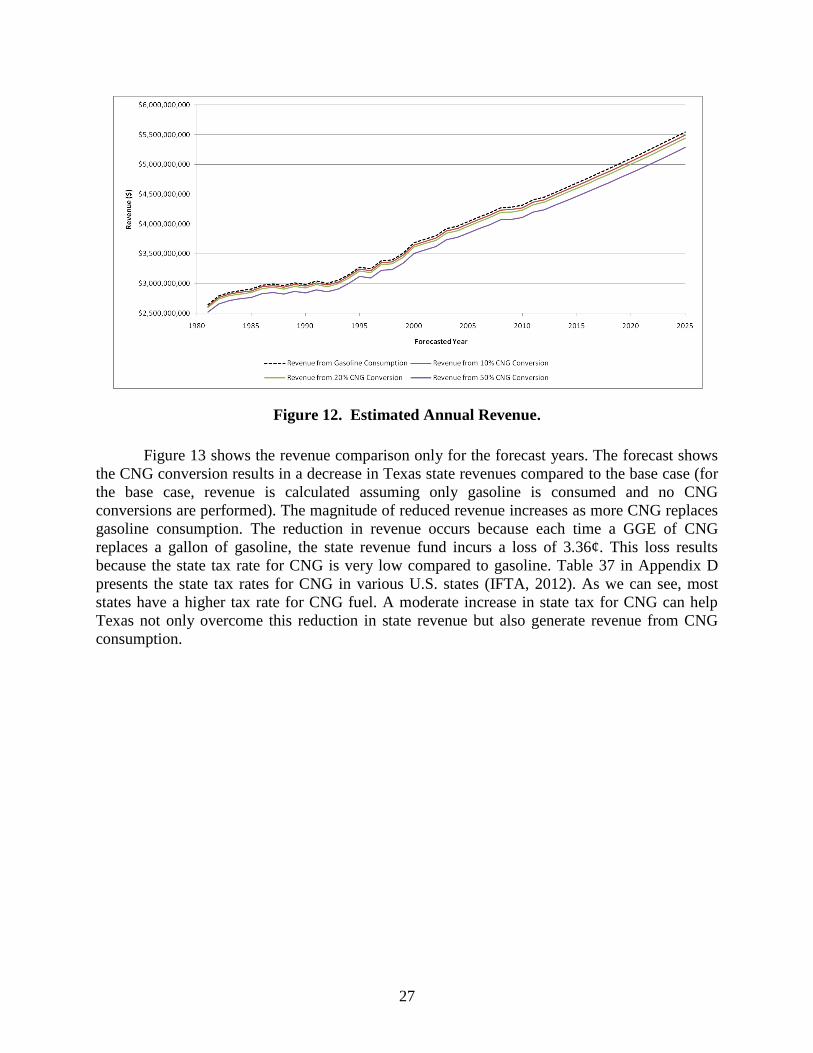
27

Figure 12. Estimated Annual Revenue.

Figure 13 shows the revenue comparison only for the forecast years. The forecast shows

the CNG conversion results in a decrease in Texas state revenues compared to the base case (for

the base case, revenue is calculated assuming only gasoline is consumed and no CNG

conversions are performed). The magnitude of reduced revenue increases as more CNG replaces

gasoline consumption. The reduction in revenue occurs because each time a GGE of CNG

replaces a gallon of gasoline, the state revenue fund incurs a loss of 3.36¢. This loss results

because the state tax rate for CNG is very low compared to gasoline. Table 37 in Appendix D

presents the state tax rates for CNG in various U.S. states (IFTA, 2012). As we can see, most

states have a higher tax rate for CNG fuel. A moderate increase in state tax for CNG can help

Texas not only overcome this reduction in state revenue but also generate revenue from CNG

consumption.

28

Figure 13. Forecast Years Annual Revenue Estimates.

Figure 14 shows the revenue comparison for the forecast year 2015 for various state tax

rate scenarios. As we can see, if the state tax rate increased from 15¢ to 18.4¢ per GGE (actually

18.36¢ per GGE), the revenue earned from CNG conversion breaks even with the gasoline tax

revenue, producing no revenue impact. If the tax rate increased from 15¢ to 20¢ per GGE, which

is the current tax rate for gasoline, more revenue can be generated compared to the base case.

The differences in revenue for different tax rate scenarios are presented in Figure 15.

Figure 14. Total revenue for different state tax on CNG.

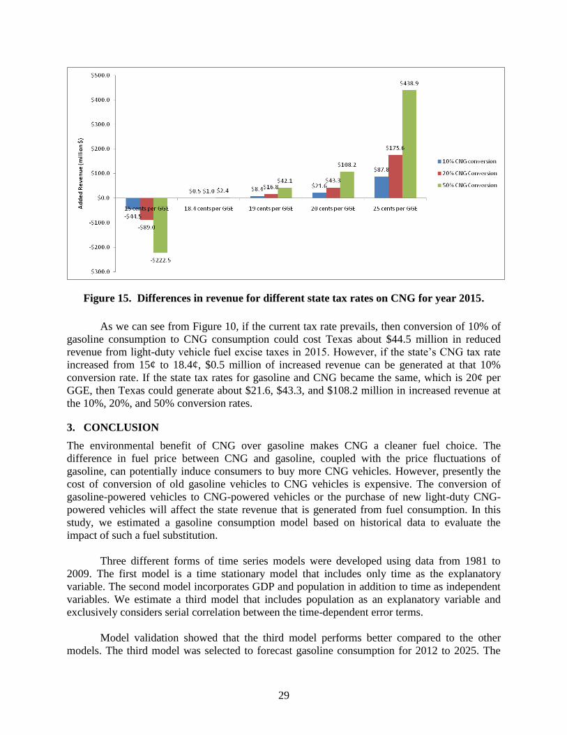
29

Figure 15. Differences in revenue for different state tax rates on CNG for year 2015.

As we can see from Figure 10, if the current tax rate prevails, then conversion of 10% of

gasoline consumption to CNG consumption could cost Texas about $44.5 million in reduced

revenue from light-duty vehicle fuel excise taxes in 2015. However, if the state’s CNG tax rate

increased from 15¢ to 18.4¢, $0.5 million of increased revenue can be generated at that 10%

conversion rate. If the state tax rates for gasoline and CNG became the same, which is 20¢ per

GGE, then Texas could generate about $21.6, $43.3, and $108.2 million in increased revenue at

the 10%, 20%, and 50% conversion rates.

3. CONCLUSION

The environmental benefit of CNG over gasoline makes CNG a cleaner fuel choice. The

difference in fuel price between CNG and gasoline, coupled with the price fluctuations of

gasoline, can potentially induce consumers to buy more CNG vehicles. However, presently the

cost of conversion of old gasoline vehicles to CNG vehicles is expensive. The conversion of

gasoline-powered vehicles to CNG-powered vehicles or the purchase of new light-duty CNG-

powered vehicles will affect the state revenue that is generated from fuel consumption. In this

study, we estimated a gasoline consumption model based on historical data to evaluate the

impact of such a fuel substitution.



variable. The second model incorporates GDP and population in addition to time as independent

variables. We estimate a third model that includes population as an explanatory variable and

exclusively considers serial correlation between the time-dependent error terms.

Model validation showed that the third model performs better compared to the other

models. The third model was selected to forecast gasoline consumption for 2012 to 2025. The

30

estimated gasoline consumption was used to calculate the state revenue generated from gasoline

consumption. Then we estimated the revenue for three scenarios where 10%, 20%, and 50% of

gasoline consumption would be replaced by CNG consumption. All these cases show that

substituting gasoline consumption with CNG would result in lower revenue for the state of Texas

if the current tax rates remain the same for the forecast years. A moderate increase in the Texas

state tax rate for CNG fuel has the potential to overcome the loss in revenue. Applying the same

state tax rate to both CNG and gasoline would result in added Texas excise tax revenue from

light-duty vehicles because Texas receives a slightly higher percentage of collected federal

excise taxes for CNG compared to gasoline.

31

CHAPTER 4. LIQUEFIED PETROLEUM GAS (LPG)

1. INTRODUCTION TO LPG

Liquefied petroleum gas (LPG), also known as propane, or butane is another alternative fuel

derived as a bi-product of natural gas production and the oil refining process. LPG is composed

of mostly propane and butane. Natural gas purification produces about 55 percent of all LPG,

while crude oil refining produces about 45 percent (Texas Comptroller of Public Accounts,

2008). Like other alternative fuels, LPG is a cleaner-burning fuel than diesel and gasoline and

90% of propane used in the U.S. comes from domestic sources (U.S. Department of Energy,

2013). LPG-fueled vehicles produce significantly lower greenhouse gas (GHG) emission

compared to conventional gasoline powered vehicles; of course, the emission reduction benefit

varies with the engine design.

The state of Texas is a proponent of the use of LPG as an alternative to gasoline. As a part of

Texas Emissions Reduction Plan, the Texas Commission on Environmental Quality (TCEQ)

administers programs that provide grants to the owners of vehicle fleets to permanently remove

diesel vehicles from the road and replace them with alternative fuel vehicles (AFVs) or hybrid

electric vehicles (HEVs). TCEQ programs include the “Alternative Fueling Facilities Program”

that provides grants for alternative fueling infrastructure and the “Emissions Reduction Incentive

Grants (ERIG) Program” that allows grants for clean vehicles and infrastructure, and the “Texas

Clean Fleet Program.” The Railroad Commission of Texas Alternative Energy Division's “Low

Emissions Alternative Fuels Equipment Initiative Program” also offers grants to buyers who

wish to replace aging medium- or heavy-duty diesel school buses or delivery vehicles with

qualified propane or natural gas vehicles that meet or exceed current U.S. Environmental

Protection Agency (EPA) emissions standards (AFDC, 2013). Additionally, LPG gas use is

encouraged by a federal tax incentive. A tax credit of $0.50 per gallon is available for LPG users

between January 1, 2005, and December 31, 2013 (U.S. DOE).

LPG is used as a fuel in the residential, commercial, industrial, and transportation sectors.

The state of Texas is the nation’s largest producer and consumer of LPG. In year 2011, Texas

consumed 500.98 million barrels of LPG for fuel, 60.4 percent of all LPG consumed in the U.S.

(U.S. Energy Information Administration, 2011). Although the transportation sector accounts for

only 0.115 percent of LPG consumption in Texas, LPG is one of the most commonly used

alternative fuels in the U.S. (EIA, 2012; NHTSA, 2002). Texas is a strong proponent of

alternative fuels and alternative fuel vehicles and mandates state agencies to purchase alternative

fuel vehicles (U.S. Department of Energy, 1999). Texas is among the three states in the U.S. that

consume the most LPG as transportation fuel and has the highest number (457) of LPG fuel

stations in the nation (AFDC, 2013). Motivated in part by the state law, the largest fleet in Texas,

operated by Texas Department of Transportation (TxDOT), has been using hundreds of LPG-

fueled and bi-fuel (LPG and gasoline) vehicles for their fleet since 1992 (U.S. DOE, 1999;

Huang et al., 1999; Werpy et al., 2010; TxDOT, 2012). However, the number of the LPG

vehicles in TxDOT’s fleet has fallen sharply from year 2001 to 2010. In fiscal year 2001,

TxDOT’s fleet included 4,677 LPG vehicles, which remained relatively stable until 2004. The

number of LPG vehicles started to drop in year 2005 (3869 LPG vehicles) and by fiscal 2010,

this portion of the fleet had dropped by 77.6 percent from 3,269 to 1,048 vehicles (Texas

Comptroller of Public Accounts, 2008; TxDOT, 2012). The availability of other alternative fuels,

http://www.tceq.state.tx.us/implementation/air/terp/tcf.html

http://www.tceq.state.tx.us/implementation/air/terp/tcf.html



32

the limited availability of public LPG fueling stations, and decisions by some equipment

manufacturers to stop producing and selling LPG vehicles, have contributed to the decreased size

of LPG fleets (Texas Comptroller of Public Accounts, 2008).

LPG is a colorless, odorless, and nontoxic gas whose boiling point is below room

temperature. The pressure at which LPG becomes liquid, called its vapor pressure, varies

depending on composition and temperature; for example, it is approximately 32 psi (220

kilopascals) for pure butane at 68 °F (20 °C), and approximately 320 psi (2.2 megapascals) for

pure propane at 131 °F (55 °C). LPG is heavier than air, unlike natural gas, and thus will flow

along floors and tend to settle in low spots. For easy transportation and storage, LPG is stored as

a liquid in a moderately low-pressure vehicle fuel tank (about 150 pounds per square inch)

(AFDC, 2013). LPG has a high-octane value compared to gasoline (104 to 112 compared with

87 to 92 for gasoline) that allows for a higher compression ratio in the engine and greater engine

efficiency (EPA, 2002; AFDC, 2013). The service life of LPG vehicles is 2-3 years longer

compared to gasoline powered vehicles and requires less frequent maintenance (AFDC, 2013). In

liquid state, LPG has the lowest flammability range of any alternative fuel and is not harmful to

soil or water. However, overfilled LPG fuel tanks have potential safety and emissions

implications (Werpy et al., 2010). The energy density of LPG is about 73% that of gasoline, thus

requiring more fuel to travel an equivalent distance (AFDC, 2013). LPG vehicles have longer

driving ranges compared to CNG vehicles. LPG vehicles can either be conversions from gasoline

vehicles or purchased from authorized vehicle dealers. Auto-manufacturers such as Ford and

General Motors offer light- and medium-duty dedicated and bi-fueled LPG vehicles (U.S. DOE,

2013). Gasoline powered vehicles can also be converted to LPG fuel use. The conversion cost of

a light-duty vehicle from gasoline to propane use ranges from $4,000 to $12,000 (AFDC, 2013).

In converted vehicles, the propane fuel system increases the weight of the vehicle by

approximately 100 pounds (EPA, 2002). There are also two types of fuel-injection systems

available: vapor injection and liquid propane injection. In both types, LPG is stored as a liquid in

a relatively low-pressure tank (AFDC, 2013).

The price of LPG fuel is relatively lower than gasoline, but higher than compressed natural

gas (CNG). U.S. DOE reported that the average LPG price in the Gulf Coast area in January

2013 was $2.17 per liquid gallon. In Texas, the State excise tax is not collected at the pump so

adding $0.15 per gallon brings the actual price to about $2.32 per gallon. If one applies the $0.50

per gallon federal tax credit, the LPG price becomes $1.80 per gallon. Gasoline fuel in the same

region was priced around $3.11 per gallon. While this might appear to be a significant LPG

price advantage, if one adjusts for the energy density of the two fuels by dividing the LPG price

by 0.73, the LPG energy density compared to gasoline, the LPG price becomes $2.49 per

equivalent gallon or about $0.62 less than gasoline fuel. However, like gasoline the price of

LPG fuel also fluctuates as it depends on a number of factors, some of them are common to all

petroleum products, and others are specific to propane (EIA, 2012). Since LPG is used not only

as a vehicle fuel but also as an energy source for home heating, and cooking, as well as, as a

replacement for chlorofluorocarbon or hydrofluorocarbon refrigerants, the market price for LPG

fuel is influenced by the product demand in the other LPG market segments. Although some

LPG is derived from natural gas, the primary source of LPG is crude oil so its cost is clearly

influenced by the cost of crude oil. The production of LPG by refineries and gas processing

plants is relatively steady year-round, however, the demand for it is subject to changes in

https://en.wikipedia.org/wiki/Vapour_pressure

https://en.wikipedia.org/wiki/Butane

https://en.wikipedia.org/wiki/Propane

https://en.wikipedia.org/wiki/Air

https://en.wikipedia.org/wiki/Natural_gas

https://en.wikipedia.org/wiki/Chlorofluorocarbon

https://en.wikipedia.org/wiki/Hydrofluorocarbon

https://en.wikipedia.org/wiki/Refrigerant

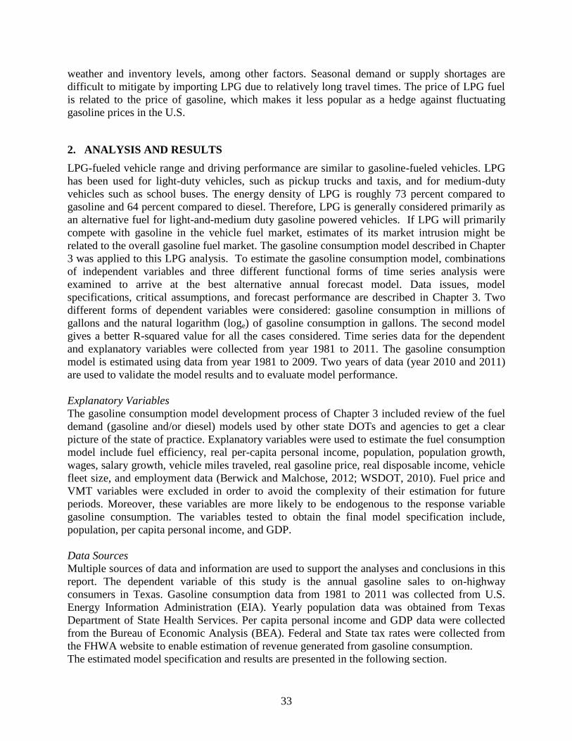
33

weather and inventory levels, among other factors. Seasonal demand or supply shortages are

difficult to mitigate by importing LPG due to relatively long travel times. The price of LPG fuel

is related to the price of gasoline, which makes it less popular as a hedge against fluctuating

gasoline prices in the U.S.


LPG-fueled vehicle range and driving performance are similar to gasoline-fueled vehicles. LPG

has been used for light-duty vehicles, such as pickup trucks and taxis, and for medium-duty

vehicles such as school buses. The energy density of LPG is roughly 73 percent compared to

gasoline and 64 percent compared to diesel. Therefore, LPG is generally considered primarily as

an alternative fuel for light-and-medium duty gasoline powered vehicles. If LPG will primarily

compete with gasoline in the vehicle fuel market, estimates of its market intrusion might be

related to the overall gasoline fuel market. The gasoline consumption model described in Chapter

3 was applied to this LPG analysis. To estimate the gasoline consumption model, combinations

of independent variables and three different functional forms of time series analysis were

examined to arrive at the best alternative annual forecast model. Data issues, model

specifications, critical assumptions, and forecast performance are described in Chapter 3. Two

different forms of dependent variables were considered: gasoline consumption in millions of

gallons and the natural logarithm (loge) of gasoline consumption in gallons. The second model

gives a better R-squared value for all the cases considered. Time series data for the dependent

and explanatory variables were collected from year 1981 to 2011. The gasoline consumption

model is estimated using data from year 1981 to 2009. Two years of data (year 2010 and 2011)

are used to validate the model results and to evaluate model performance.


The gasoline consumption model development process of Chapter 3 included review of the fuel

demand (gasoline and/or diesel) models used by other state DOTs and agencies to get a clear

picture of the state of practice. Explanatory variables were used to estimate the fuel consumption

model include fuel efficiency, real per-capita personal income, population, population growth,

wages, salary growth, vehicle miles traveled, real gasoline price, real disposable income, vehicle

fleet size, and employment data (Berwick and Malchose, 2012; WSDOT, 2010). Fuel price and

VMT variables were excluded in order to avoid the complexity of their estimation for future

periods. Moreover, these variables are more likely to be endogenous to the response variable

gasoline consumption. The variables tested to obtain the final model specification include,

population, per capita personal income, and GDP.

Data Sources


report. The dependent variable of this study is the annual gasoline sales to on-highway

consumers in Texas. Gasoline consumption data from 1981 to 2011 was collected from U.S.

Energy Information Administration (EIA). Yearly population data was obtained from Texas

Department of State Health Services. Per capita personal income and GDP data were collected

from the Bureau of Economic Analysis (BEA). Federal and State tax rates were collected from

the FHWA website to enable estimation of revenue generated from gasoline consumption.

The estimated model specification and results are presented in the following section.

34

Revenue Forecast

Using the gasoline consumption forecast presented in Chapter 3, current Federal and Texas State

tax rates and the time series model with explanatory variables (model 3) are used to estimate the

revenue generated from gasoline consumption. The tax rates used in revenue calculation are

presented in Table 19.

Table 13. Tax rates used in revenue calculation.



Gasoline LPG

$/gallon $/gallon

Federal 0.184 0.136

State 0.200 0.150


[Texas receives 83.9% of Federal Tax from

Gasoline and 88.4% of Federal Tax from LPG]

Federal 0.154 0.120

State 0.200 0.150

Adjusting for Energy Equivalent Volumes

[LPG contains 73% of the energy per gasoline

gallon]

Federal 0.154 0.165

State 0.200 0.205

Effective Texas Rate Per Liquid Gallon

Total $/gallon 0.354 0.370

The current nominal excise tax rates shown in Table 19 are adjusted to account for the

fractions of collected federal taxes that are currently being returned to the State of Texas,

specifically 83.9% of federal gasoline taxes and 88.4% of federal taxes for LPG. Additionally,

LPG is taxed and sold as a liquid like gasoline, but an LPG gallon contains approximately 73

percent of the energy contained in a gallon of gasoline, so consumers must purchase more than a

gallon of LPG to travel the same distance as would be possible with a gallon of gasoline. This

adjustment for “energy density” is also applied in Table 4 and the cumulative effect of the two

“adjustments” produces an effective excise tax for LPG that is higher than gasoline. The

effective tax rates show that almost 1.6 cents more tax would be collected for each gasoline

gallon equivalent (GGE) of LPG fuel compared to each gallon of gasoline. Additionally,

although current federal law (through 31 December 2013) provides a $0.50 per GGE Alternative

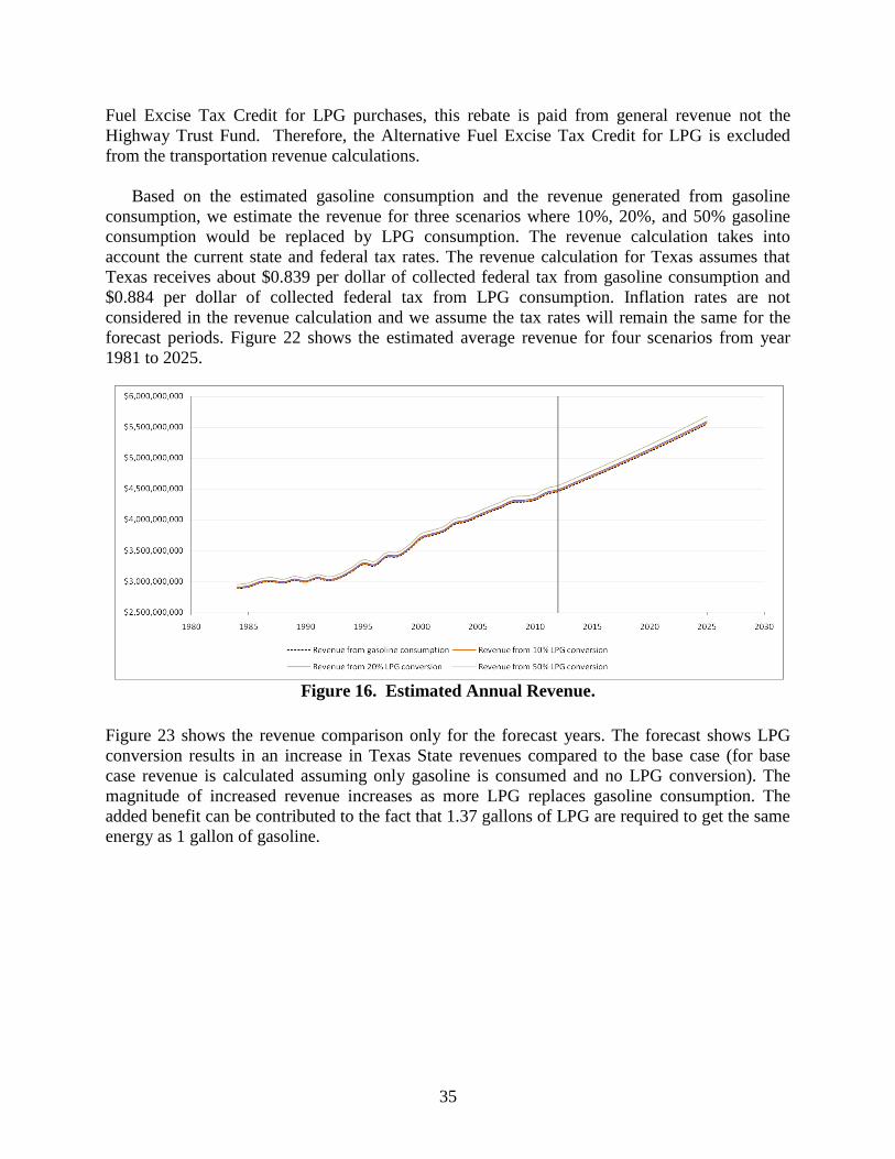
35

Fuel Excise Tax Credit for LPG purchases, this rebate is paid from general revenue not the

Highway Trust Fund. Therefore, the Alternative Fuel Excise Tax Credit for LPG is excluded

from the transportation revenue calculations.

Based on the estimated gasoline consumption and the revenue generated from gasoline

consumption, we estimate the revenue for three scenarios where 10%, 20%, and 50% gasoline

consumption would be replaced by LPG consumption. The revenue calculation takes into

account the current state and federal tax rates. The revenue calculation for Texas assumes that

Texas receives about $0.839 per dollar of collected federal tax from gasoline consumption and

$0.884 per dollar of collected federal tax from LPG consumption. Inflation rates are not

considered in the revenue calculation and we assume the tax rates will remain the same for the

forecast periods. Figure 22 shows the estimated average revenue for four scenarios from year

1981 to 2025.

Figure 16. Estimated Annual Revenue.

Figure 23 shows the revenue comparison only for the forecast years. The forecast shows LPG

conversion results in an increase in Texas State revenues compared to the base case (for base

case revenue is calculated assuming only gasoline is consumed and no LPG conversion). The

magnitude of increased revenue increases as more LPG replaces gasoline consumption. The

added benefit can be contributed to the fact that 1.37 gallons of LPG are required to get the same

energy as 1 gallon of gasoline.

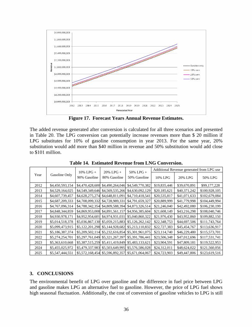
36

Figure 17. Forecast Years Annual Revenue Estimates.

The added revenue generated after conversion is calculated for all three scenarios and presented

in Table 20. The LPG conversion can potentially increase revenues more than $ 20 million if

LPG substitutes for 10% of gasoline consumption in year 2013. For the same year, 20%

substitution would add more than $40 million in revenue and 50% substitution would add close

to $101 million.

Table 14. Estimated Revenue from LNG Conversion.

3. CONCLUSIONS

The environmental benefit of LPG over gasoline and the difference in fuel price between LPG

and gasoline makes LPG an alternative fuel to gasoline. However, the price of LPG fuel shows

high seasonal fluctuation. Additionally, the cost of conversion of gasoline vehicles to LPG is still

10% LPG 20% LPG 50% LPG

2012 $4,450,593,154 $4,470,428,600 $4,490,264,046 $4,549,770,382 $19,835,446 $39,670,891 $99,177,228 2013 $4,529,164,025 $4,549,349,646 $4,569,535,266 $4,630,092,129 $20,185,621 $40,371,242 $100,928,105 2014 $4,607,739,457 $4,628,275,274 $4,648,811,091 $4,710,418,541 $20,535,817 $41,071,633 $102,679,084 2015 $4,687,209,333 $4,708,099,332 $4,728,989,331 $4,791,659,327 $20,889,999 $41,779,998 $104,449,994 2016 $4,767,096,314 $4,788,342,354 $4,809,588,394 $4,873,326,514 $21,246,040 $42,492,080 $106,230,199 2017 $4,848,344,859 $4,869,953,008 $4,891,561,157 $4,956,385,604 $21,608,149 $43,216,298 $108,040,746 2018 $4,930,978,171 $4,952,954,601 $4,974,931,031 $5,040,860,322 $21,976,430 $43,952,860 $109,882,150 2019 $5,014,518,378 $5,036,867,130 $5,059,215,883 $5,126,262,142 $22,348,753 $44,697,506 $111,743,764 2020 $5,099,473,915 $5,122,201,298 $5,144,928,682 $5,213,110,832 $22,727,383 $45,454,767 $113,636,917 2021 $5,186,387,374 $5,209,502,114 $5,232,616,854 $5,301,961,075 $23,114,740 $46,229,480 $115,573,701 2022 $5,274,254,701 $5,297,761,049 $5,321,267,397 $5,391,786,441 $23,506,348 $47,012,696 $117,531,741 2023 $5,363,610,668 $5,387,515,259 $5,411,419,849 $5,483,133,621 $23,904,591 $47,809,181 $119,522,953 2024 $5,455,025,972 $5,479,337,983 $5,503,649,995 $5,576,586,028 $24,312,011 $48,624,022 $121,560,056 2025 $5,547,444,551 $5,572,168,454 $5,596,892,357 $5,671,064,067 $24,723,903 $49,447,806 $123,619,516

10% LPG + 90% Gasoline

Gasoline Only 20% LPG +

80% Gasoline 50% LPG +

50% Gasoline

Additional Revenue generated from LPG use Year

37

expensive. The conversion of gasoline powered vehicles to LPG powered vehicles or the

purchase of new LPG vehicles will change the State revenue that is generated from fuel taxes.

In this study, we estimate a gasoline consumption model based on historical data to evaluate

the impact of such substitution. Three different forms of time series models are developed using

data from years 1981 to 2009. The first model is a trend stationary model that includes only time

as the explanatory variable. The second model incorporates per capita personal income and

population in addition to time as independent variables. We estimate a third model that

exclusively considers serial correlation between the error terms.

Model validation shows that the third model performs better compared to the first and second

models. The third model is selected to forecast gasoline consumption for year 2012 to 2025. The

estimated gasoline consumption is used to calculate the state revenue generated. Then we

estimate the revenue for three scenarios where 10%, 20%, and 50% gasoline consumption would

be replaced by LPG consumption. All these cases show that substitution of gasoline demand by

LPG would result in higher revenue for the state of Texas contingent upon present tax rates

remaining the same for the forecast years.

38

CHAPTER 5. CONCLUSIONS AND RECOMMENDATIONS

The transportation sector accounts for more than half of world oil consumption (Hirsch et al.,

2005). In the United States, about 90% of the fuel used for on-road vehicular travel is petroleum-

based, which includes gasoline and diesel (Ribeiro et al., 2007). Alternative fuel vehicles (AFV)

offer solutions to both the transportation sector’s dependence on oil and air quality concerns.

Vehicle characteristics and movement behavior of freight hauling trucks make them an

attractive market for promoting alternative fuels. A variety of alternative fuels and advanced

propulsion technologies have been explored for heavy trucks, including battery electric, hybrid

electric, biodiesel, ethanol, propane, dimethyl ether (DME), LNG, CNG, and both liquefied and

gaseous hydrogen (Myers et al., 2012). Natural gas is one of the cleanest burning fuels and can

be used in vehicles in the form of either CNG or LNG. LNG is more suitable for heavy-duty

vehicles because it has much higher energy density than CNG and can provide a safe traveling

distance of up to 600 miles between refueling stops (Myers et al., 2012).



variable. The second model incorporates per capita personal income and population in addition

to time as independent variables. We estimate a third model that exclusively considers serial

correlation between the error terms.

Due to cost of fuel conversion and physical size of LNG on-board vehicle fuel tanks,

trucks rather than passenger cars are the most suitable vehicle type for LNG fueling. Since the

truck fleet is largely fueled by diesel, this report forecasts diesel consumption through 2025 and

then considers the impacts of converting from diesel to LNG at the rates of 10, 20, and 50%.

Current tax rates for diesel and LNG fuel are $0.44 and $0.269 per liquid gallon, including both

Texas state and federal excise taxes. However, Texas receives approximately 87.9% of the

federal tax collected in Texas for both fuels, yielding the effective tax rates of $0.4145 and

$0.2546 for diesel and LNG, respectively. LNG provides only about 60% of the energy of an

equivalent volume of diesel, meaning the user must purchase 1.67 gallons of LNG to travel the

same distance as on 1 gallon of diesel. Because users must buy more LNG to go the same

distance, after adjusting for the fraction of federal tax received by Texas, the effective tax rates

are $0.414 per gallon of diesel and $0.424 per energy equivalent gallon for LNG. Although the

trucking community has some interest in LNG, this interest seems to be based primarily on LNG

prices being less than diesel fuel. Current pump prices at Texas retail outlets selling LNG fuel

are approximately $2.75 per gallon compared to about $3.90 per gallon for diesel. However, the

LNG energy equivalent price (computed by dividing $2.75 by 0.6) is $4.58 per gallon. Current

federal law (through December 31, 2013) provides a $0.50 per gallon tax rebate for LNG

purchases. This rebate is paid from general revenue, not the Highway Trust Fund. All these cases

show that substituting LNG for diesel would result in greater revenue for the state of Texas

(contingent upon the present tax rates remaining the same for the forecast years).

Light-duty vehicles, including passenger cars and light-duty trucks, are the most suitable

vehicles for CNG fueling because the driving ranges of CNG-fueled vehicles are limited. CNG

has only 25% of the energy density of diesel fuel. Since the light-duty vehicle fleet is largely

39

fueled by gasoline, this report forecasts gasoline consumption through 2025 and then considers

the impacts of converting from gasoline to CNG at the rates of 10, 20, and 50%. The current tax

rate for gasoline is $0.384 per liquid gallon and for CNG fuel is $0.333 per GGE (this figure

includes both Texas state and federal excise taxes). However, Texas receives approximately

83.9% of the federal tax collected in Texas for gasoline and approximately 93.3% of the federal

CNG tax collected in Texas. Applying these adjustments, the effective tax rates are $0.354 and

$0.321 for gasoline and CNG, respectively. Given the current effective excise tax rates for

gasoline versus CNG, TxDOT will lose revenue as CNG replaces gasoline as a vehicle fuel.

Based upon current federal and state tax rates and percentages of federal taxes returned to Texas,

increasing the current $0.15 per GGE CNG state tax rate to $0.1836 per GGE will provide

equivalent effective tax rates for gasoline and CNG.

Interest in CNG within the light-duty vehicle community seems to be based primarily on

CNG reducing consumer costs. Current pump prices are favorable: Texas retail outlets are

selling CNG fuel for $2.10 per GGE compared to about $3.50 per gallon for gasoline. In Texas,

the state excise tax is not collected at the pump, so adding $0.15 per gallon brings the actual

price to about $2.25 per GGE. Additionally, current federal law (through December 31, 2013)

provides a $0.50 per GGE Alternative Fuel Excise Tax Credit for CNG purchases. This rebate is

paid from general revenue, not the Highway Trust Fund. The cost to convert a currently owned

or newly purchased light-duty vehicle to CNG is approximately $10,000 or more. If an LNG user

drives 12,000 miles per year, has an overall fuel economy of 28 miles per gallon, saves $1.25 per

gallon using CNG instead of gasoline, and receives the $0.50 per GGE federal tax credit, then

(ignoring inflation) almost seven years will be required to amortize the CNG conversion cost.

The difference in fuel price between CNG and gasoline, coupled with the price fluctuations of

gasoline, can potentially induce consumers to buy more CNG vehicles. However, presently the

cost of conversion of old gasoline vehicles to CNG vehicles is expensive.

All these cases show that substituting gasoline consumption with CNG would result in

lower revenue for the state of Texas if the current tax rates remain the same for the forecast

years. A moderate increase in the Texas state tax rate for CNG fuel has the potential to overcome

the loss in revenue. Applying the same state tax rate to both CNG and gasoline would result in

added Texas excise tax revenue from light-duty vehicles because Texas receives a slightly higher

percentage of collected federal excise taxes for CNG compared to gasoline.

Although the primary market for LPG has traditionally been residential heating, it is a

viable fuel for light and medium duty vehicles including passenger cars, and light-and-medium

duty trucks since the energy content of LPG is generally about 73% that of gasoline or 64% of

diesel fuel. Current nominal tax rates for gasoline and LPG fuel are $0.384 and $0.286 per liquid

gallon including both Texas State and federal excise taxes. However, Texas receives

approximately 83.9 percent of the federal gasoline tax collected in Texas and approximately 88.4

percent of the federal LPG tax collected in Texas. Adjusting the nominal rates for the fractions

of federal taxes returned to Texas and adjusting for the fact that LPG contains about 73 percent

of the energy of gasoline per unit volume the effective tax rates are $0.354 and $0.370 for

gasoline and LPG, respectively. Interest within the light- and medium-duty vehicle community in

LPG seems to be based primarily on LPG reducing consumer costs. Current pump prices are

slightly favorable. Gulf coast retail outlets are selling LPG fuel for $2.17 per gallon. In Texas,

the State excise tax is not collected at the pump for LPG so adding $0.15 per gallon brings the

actual price to about $2.32 per gallon. The federal tax credit of $0.50 per gallon of LPG fuel

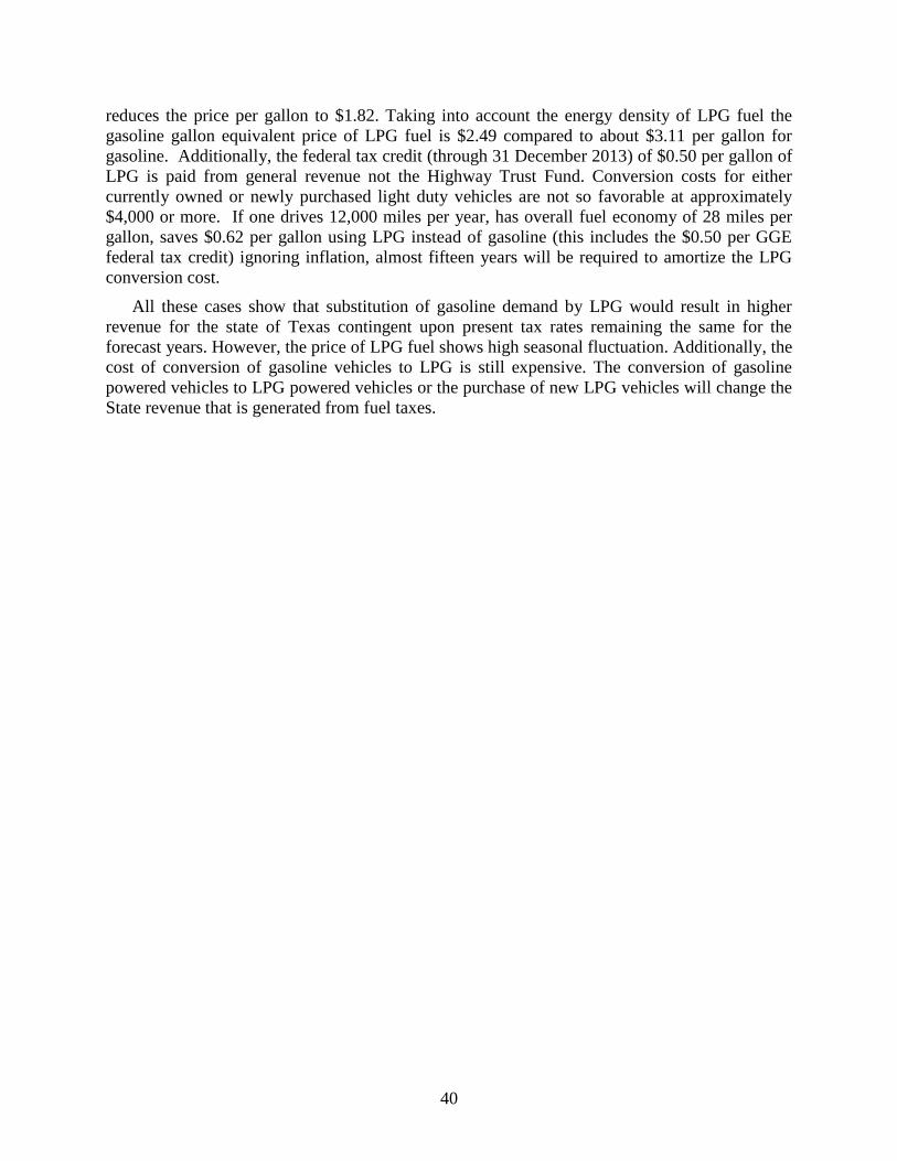
40

reduces the price per gallon to $1.82. Taking into account the energy density of LPG fuel the

gasoline gallon equivalent price of LPG fuel is $2.49 compared to about $3.11 per gallon for

gasoline. Additionally, the federal tax credit (through 31 December 2013) of $0.50 per gallon of

LPG is paid from general revenue not the Highway Trust Fund. Conversion costs for either

currently owned or newly purchased light duty vehicles are not so favorable at approximately

$4,000 or more. If one drives 12,000 miles per year, has overall fuel economy of 28 miles per

gallon, saves $0.62 per gallon using LPG instead of gasoline (this includes the $0.50 per GGE

federal tax credit) ignoring inflation, almost fifteen years will be required to amortize the LPG

conversion cost.

All these cases show that substitution of gasoline demand by LPG would result in higher

revenue for the state of Texas contingent upon present tax rates remaining the same for the

forecast years. However, the price of LPG fuel shows high seasonal fluctuation. Additionally, the

cost of conversion of gasoline vehicles to LPG is still expensive. The conversion of gasoline

powered vehicles to LPG powered vehicles or the purchase of new LPG vehicles will change the

State revenue that is generated from fuel taxes.

41

REFERENCES

Alternative Fuel Data Center (AFDC), U.S. DOE, 2013. Texas Laws and Incentives. Retrieved

March 20, 2013, from http://www.afdc.energy.gov/laws/laws/TX

Alternative Fuel Data Center (AFDC), U.S. DOE, 2013, Natural Gas Vehicles, Retrieved March

25, 2013, from http://www.afdc.energy.gov/vehicles/natural_gas.html

Alternative fuels data center (AFDC), 2013. Retrieved April 23, 2013 from

http://www.afdc.energy.gov/vehicles/propane_conversions.html

Alternative fuel data center (AFDC), 2013. Retrieved April 23, 2013 from

http://www.afdc.energy.gov/vehicles/propane.html

Berwick, M., Malchose, D., 2012, Forecasting North Dakota fuel tax revenue and license and

registration fee revenue, Upper Great Plains Transportation Institute, North Dakota State

University, Fargo, North Dakota.

BEA, 2013, Regional data, Retrieved March 20, 2013,

from http://www.bea.gov/newsreleases/regional/lapi/lapi_newsrelease.htm

BTS, 2009, 2007 Commodity Flow Survey United States, Retrieved March 20, 2013, from

http://www.rita.dot.gov/bts/sites/rita.dot.gov.bts/files/publications/commodity_flow_survey/final

_tables_december_2009/index.html

CNG California Retrieved March 20, 2013, from http://www.cngcalifornia.com/cng-faqs.asp

Davis, Stacy C., Susan W. Diegel, and Robert G. Boundy. 2012. Transportation Energy Data

Book: Edition 30, Retrieved April 14, 2013, from

http://cta.ornl.gov/data/tedb31/Edition31_Full_Doc.pdf

Department of Energy Alternative Fuel Data Center, 2013. LPG Incentives, retrieved April 23,

2013 from http://www.afdc.energy.gov/laws/laws/TX/tech/3254

EIA, 2013, Texas No 2 Diesel Sales/Deliveries to On-highway Consumers, Retrieved March 20,

2013, from http://www.eia.gov/tools/faqs/faq.cfm?id=10&t=10

Energy Information Administration (EIA), 2009, Propane from natural gas or Oil, in Propane

Explained. Retrieved April 23, 2013 from,

http://tonto.eia.doe.gov/energyexplained/index.cfm?page=propane_home

Energy Modeling Forum (EMF), 1992, International Oil Supplies and Demands, EMF Report 11

(II), Stanford University.

EPA, 2010, Sources of Greenhouse Gas Emissions, Retrieved March 20, 2013, from

http://www.epa.gov/climatechange/ghgemissions/sources.html

EPA, 2002, Clean Alternative Fuels: Liquefied Natural Gas, Retrieved March 20, 2013, from

http://www.afdc.energy.gov/pdfs/epa_lng.pdf

http://www.afdc.energy.gov/laws/laws/TX

http://www.afdc.energy.gov/vehicles/propane_conversions.html

http://www.afdc.energy.gov/vehicles/propane.html

http://www.bea.gov/newsreleases/regional/lapi/lapi_newsrelease.htm

http://www.cngcalifornia.com/cng-faqs.asp

http://cta.ornl.gov/data/tedb31/Edition31_Full_Doc.pdf

http://www.afdc.energy.gov/laws/laws/TX/tech/3254

http://www.eia.gov/tools/faqs/faq.cfm?id=10&t=10

http://www.epa.gov/climatechange/ghgemissions/sources.html

http://www.afdc.energy.gov/pdfs/epa_lng.pdf

42

FHWA, 2012, Highway statistics 2010. Retrieved March 20, 2013, from

http://www.fhwa.dot.gov/policyinformation/statistics/2010/vm1.cfm

FHWA, 2012, Highway statistics 2011. Retrieved March 20, 2013, from

http://www.fhwa.dot.gov/policyinformation/statistics/2011/mf121t.cfm

FHWA, 2011, Financing Federal-aid Highways, Retrieved March 20, 2013,

http://www.fhwa.dot.gov/reports/fifahiwy/fifahi05.htm

Freightliner Trucks, 2013, Natural Gas: Technology You Can Bank On, Retrieved March 25,

2013, from http://www.freightlinertrucks.com/Trucks/Alternative-Power-Trucks/Natural-

Gas/Cascadia-113-NG

GAO, 2010, Report to the Congressional Requesters, Retrieved March 20, 2013, from

http://www.gao.gov/new.items/d10780.pdf

Greene, D. L., Leiby, P. N., 1993, The Social Costs to the U.S. of Monopolization of the World

Oil Market, 1972–1991, Oak Ridge National Laboratory, ORNL-6744.

Hirsch, R. L., Bezdek, R.; Wendling, R., 2005, Peaking of World Oil Production: Impacts,

Mitigation, and Risk Management. Science Applications International

Corporation/U.S.Department of Energy, National Energy Technology Laboratory.

IFTA Fuel Tax Rate Sheet, 2012, Retrieved March 20, 2013, from

http://tax.illinois.gov/taxforms/misc/mft/MFUT-15-T.pdf

IFTA Fuel Tax Rate Sheet, 2012, Retrieved March 20, 2013, from


National Highway Traffic Safety Administration (NHTSA), 2002, Retrieved April 23, 2013 from

http://stnw.nhtsa.gov/cars/rules/rulings/cafe/alternativefuels/

Nesbitt, K., Sperling, D., 1998, Myths regarding alternative fuel vehicle demand by light-duty

vehicle fleets. Transportation Research Part D, 3( 4), 259-269, 1998

NHTSA, 2002, Report to congress, Effects of alternative fuels act CAFÉ incentives policy,

Retrieved March 20, 2013, from

http://www.nhtsa.gov/cars/rules/rulings/cafe/alternativefuels/index.htm

NGV America, 2012, Fact sheet: Converting light duty vehicles to natural gas, Retrieved April

14, 2013, from http://www.ngvc.org/pdfs/FAQs_Converting_to_NGVs.pdf

Ribeiro, K. S., Kobayashi,S., Beuthe, M., Gasca, J., Greene, D., Lee, D. S. , Muromachi, Y. ,

Newton, P. J. , Plotkin, S. , Sperling, D. , Wit, R. , Zhou, P. J. ,2007, Transport and its

Infrastructure. In Climate Change 2007: Mitigation. Contribution of Working Group III to

the Fourth Assessment Report of the Intergovernmental Panel on Climate Change [B. Metz,

O.R. Davidson, P.R. Bosch, R. Dave, L.A. Meyer (eds)], Cambridge University Press,

Cambridge, United Kingdom and New York, NY, USA. Retrieved March 20, 2013,

from http://www.ipcc.ch/publications_and_data/ar4/wg3/en/ch5.html

http://www.fhwa.dot.gov/policyinformation/statistics/2010/vm1.cfm

http://www.fhwa.dot.gov/reports/fifahiwy/fifahi05.htm


http://stnw.nhtsa.gov/cars/rules/rulings/cafe/alternativefuels/

http://www.nhtsa.gov/cars/rules/rulings/cafe/alternativefuels/index.htm

http://www.ngvc.org/pdfs/FAQs_Converting_to_NGVs.pdf

http://www.ipcc.ch/publications_and_data/ar4/wg3/en/ch5.html

43

Semin, R. A., 2008. A technical review of compressed natural gas as an alternative fuel for

internal combustion engines, American Journal of Engineering and Applied Sciences 1 (4):

302–311.

Silverstein, K., 2013, Forbes, Retrieved March 20, 2013, from

http://www.forbes.com/sites/kensilverstein/2012/12/15/all-roads-lead-to-natural-gas-fueled-

cars-and-trucks/.

Statistics Brain, Retrieved April 14, 2013, from

http://www.statisticbrain.com/gas-station-statistics/

Sutherland, T. F., 2011, National Geographic, Retrieved March 20, 2013, from

http://www.greatenergychallengeblog.com/2011/05/04/lng-for-truck-fuel%E2%80%A6the-

time-is-right/#comments

Texas Gas Service, Retrieved April 14, 2013, from

https://www.texasgasservice.com/en/SaveEnergyAndMoney/NaturalGasVehicles/FAQ.aspx

Texas railroad commission alternative fuels research and education division, Retrieved April 14,

http://www.propane.tx.gov/rebate_program/rebatepdfs/save55cents.pdf

Texas comptroller of public accounts, 2008. Research and Analysis Division, Chapter 6,

Liquefied Petroleum Gas in The Energy Report, pp. 81–88, Retrieved April 23 from

http://www.window.state.tx.us/specialrpt/energy/pdf/96-1266EnergyReport.pdf

Texas Department of Health Statistics, 2012, Population Data for Texas, Retrieved March 20,

2013, from http://soupfin.tdh.state.tx.us/people.htm

Texas department of transportation (TxDOT), 2012. Inside TxDOT, retrieved April 23, 2013

from http://www.txdot.gov/inside-txdot/division/environmental/programs/alternative-

fuels.html

Texas railroad commission alternative fuels research and education division, 2013. Retrieved

April 23 from, http://www.rrc.state.tx.us/programs/save55cents.pdf

TIAX, 2013, U.S. and Canadian Natural Gas Vehicle Market Analysis: Liquefied natural gas

Market Infrastructure. Retrieved March 20, 2013, from

http://anga.us/media/content/F7D3861D-9ADE-7964-

0C27B6F29D0A662B/files/LNG%20Infrastructure.pdf

U.S. DOE, 2009, Research and Development Opportunities for Heavy Duty Trucks,

http://www1.eere.energy.gov/vehiclesandfuels/pdfs/truck_efficiency_paper_v2.pdf

U.S. DOE, 2013, Natural Gas, Retrieved March 20, 2013, from

http://www.fueleconomy.gov/feg/bifueltech.shtml

U.S. DOE, 2009, Alternative Fuels and Federal Fleet Vehicle FAQs. Retrieved March 20, 2013,

from http://www1.eere.energy.gov/femp/pdfs/federal_fleet_faq.pdf

http://www.forbes.com/sites/kensilverstein/2012/12/15/all-roads-lead-to-natural-gas-fueled-cars-and-trucks/

http://www.forbes.com/sites/kensilverstein/2012/12/15/all-roads-lead-to-natural-gas-fueled-cars-and-trucks/

http://www.statisticbrain.com/gas-station-statistics/

http://www.greatenergychallengeblog.com/2011/05/04/lng-for-truck-fuel%E2%80%A6the-time-is-right/#comments

http://www.greatenergychallengeblog.com/2011/05/04/lng-for-truck-fuel%E2%80%A6the-time-is-right/#comments

https://www.texasgasservice.com/en/SaveEnergyAndMoney/NaturalGasVehicles/FAQ.aspx

http://www.propane.tx.gov/rebate_program/rebatepdfs/save55cents.pdf

http://www.txdot.gov/inside-txdot/division/environmental/programs/alternative-fuels.html

http://www.txdot.gov/inside-txdot/division/environmental/programs/alternative-fuels.html

http://www.rrc.state.tx.us/programs/save55cents.pdf

http://www1.eere.energy.gov/vehiclesandfuels/pdfs/truck_efficiency_paper_v2.pdf

http://www.fueleconomy.gov/feg/bifueltech.shtml

http://www1.eere.energy.gov/femp/pdfs/federal_fleet_faq.pdf

44

U.S. Department of Energy, 2013. Save money. Retrieved April 14, 2013, from

http://www.fueleconomy.gov/feg/savemoney.shtml

U.S. Department of Energy, 2013. Clean cities 2013 vehicle buyer’s guide. Retrieved April 23

from, http://www.afdc.energy.gov/uploads/publication/55873.pdf

U.S. Energy Information Administration. State Energy Data 2011: Consumption. Retrieved July

29, 2013 from http://www.eia.gov/state/seds/sep_use/notes/use_print.pdf

U.S. Department of Energy, Retrieved April 14, 2013, from


U.S. Energy Information Administration, Retrieved April 14, 2013, from

http://www.eia.gov/energy_in_brief/article/foreign_oil_dependence.cfm

U.S. Government Accountability Office, 2010, Report to the Congressional Requesters,

Retrieved March 20, 2013, from http://www.gao.gov/new.items/d10780.pdf

U.S. Government Accountability Office, 2010, Report to the Congressional Requesters,

Retrieved March 20, 2013, from http://www.gao.gov/new.items/d10780.pdf

U.S. Department of Energy Alternative Fuel Data Center, Retrieved March 20, 2013, from

http://www.afdc.energy.gov/laws/law/TX/9457

The Wall Street Journal, 2012, Retrieved March 20, 2013, from

http://online.wsj.com/article/SB10001424052702304707604577422192910235090.html.

Washington State Department of Transportation (WSDOT). 2010, Statewide Fuel Consumption

Forecast Models 2010.

Werpy, M. R., Burnham,A., Bertram, K., 2010. Propane vehicles: status, challenges, and

opportunities, Center for transportation research, Energy systems division, Argonne national

laboratory.

Wooldridge, J. M., 2006, Introductory Econometrics—A Modern Approach, Thomson South

Western.

Yacobucci, B. D., 2011, Natural Gas Passenger Vehicles: Availability, Cost, and Performance,

Congressional Research Service Report to Congress. Retrieved April 14, 2013, from

http://waxman.house.gov/sites/waxman.house.gov/files/CRS_Report_Natural_Gas_Vehicles.

pdf

Yeh, S., 2007, An Empirical Analysis on the Adoption of Alternative Fuel Vehicles: The Case of

Natural Gas Vehicles. Energy Policy, 35:5865–75.


http://www.afdc.energy.gov/uploads/publication/55873.pdf

http://www.eia.gov/state/seds/sep_use/notes/use_print.pdf


http://www.eia.gov/energy_in_brief/article/foreign_oil_dependence.cfm

http://www.afdc.energy.gov/laws/law/TX/9457

http://waxman.house.gov/sites/waxman.house.gov/files/CRS_Report_Natural_Gas_Vehicles.pdf

http://waxman.house.gov/sites/waxman.house.gov/files/CRS_Report_Natural_Gas_Vehicles.pdf

45

APPENDIX

APPENDIX A

Table 15. Listing of Texas Diesel Consumption, Per Capita Personal Income and

Population Data (1984–2011).

year Texas Diesel Consumption

(Gallons)

Per Capita Income

($)

Population

(million)

GDP

($Million)

1984 1514092000 13377 16.007 2030.73

1985 1550447000 14110 16.273 2452.35

1986 1437192000 14182 16.561 2600.85

1987 1319054000 14453 16.622 2648.83

1988 1296067000 15245 16.667 2886.37

1989 1387059000 16165 16.807 3072.24

1990 1384705000 17260 16.987 2957.21

1991 1554493000 17763 17.349 3006.67

1992 1575936000 18765 17.656 3273.54

1993 1686844000 19413 18.031 3499.52

1994 1916678000 20161 18.378 3789.43

1995 1946843000 21070 18.724 3935.74

1996 2156993000 22260 19.128 4164.01

1997 2250646000 23812 19.439 4437.75

1998 2433408000 25376 19.760 4759.90

1999 2538263000 26399 20.044 5077.25

2000 2793809000 28506 20.852 5515.13

2001 2976807000 29185 21.325 6021.60

2002 3093602000 28966 21.780 6342.86

2003 2991379000 29622 22.119 6706.04

2004 3464411000 31115 22.490 7310.64

2005 3611156000 33220 22.860 7628.85

2006 3962862000 35287 23.508 7827.80

2007 4234133000 37098 23.904 8244.89

2008 4186631000 39615 24.327 9036.79

2009 3711173000 36595 24.782 9685.53

2010 3849991000 38222 25.146 10544.14

2011 4114193000 40147 25.675 11474.04

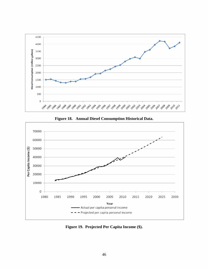
46

Figure 18. Annual Diesel Consumption Historical Data.

Figure 19. Projected Per Capita Income ($).

47

Figure 20. Projected Texas Population.

Figure 21. Projected Texas GDP.

0.000

5.000

10.000

15.000

20.000

25.000

30.000

35.000

1980 1985 1990 1995 2000 2005 2010 2015 2020 2025 2030

Po

pu

lati

on

(m

illio

n)

Year

Actual Population

Projected Population

48

APPENDIX B

Diesel ConsumptionValidation/Model Performance Evaluation

We first plot the residuals (difference between the estimated diesel consumption and the actual

diesel consumption) of the estimated models to visually examine the residuals’ distribution. The

residual plot for the first model (Figure B1) shows that most of the residuals for the first model

are located above zero (over-estimating consumption). The residuals of the adjacent periods are

observed to have the same sign and also exhibit stickiness between the adjacent periods,

indicating the presence of serial correlation between the error terms of this model. On the other

hand, the residual distribution for Model 2 (Figure B2) shows a fairly random scatter plot around

zero. Very few adjacent residuals are observed to have similar values and display less stickiness

compared to the first model, indicating that the explanatory variables remove most of the serial

correlation. The magnitudes of the residuals are also smaller compared to the first model

residuals. The third model residual plot (Figure B3) also shows a random scatter plot around

zero. However, the magnitudes of the residuals are higher compared to the second model.

Figure 22. Residual Plot for Time Stationary Model (Model 1).

Figure 23. Residual Plot for Time Series Model with Explanatory Variables (Model 2).

49

Figure 24. Residual Plot for First-Order Autoregressive Model (Model 3).

The estimated coefficients for the models are used to forecast the diesel consumption for

year 2010 and 2011. The forecasted values are compared with the actual diesel consumption data

to calculate the performance measures. The calculated performance measures for the models are

presented in Tables 22-24.

Table 16. Model 1 Performance Measures

Model 1: Trend-Stationary Model

ln (Diesel Consumption)

∑

∑

Forecasted Actual

22.218 22.071 0.146 0.021

22.268 22.138 0.131 0.017

0.277 0.038


Model 2: Time Series Model with Exogenous Variable

ln (Diesel Consumption) ∑

∑

Forecasted Actual

22.108 22.071 0.037 0.001

22.179 22.138 0.041 0.002

0.078 0.003

50


Model 3: First-Order Autoregressive Time Series Model

ln (Diesel Consumption)

∑

∑

Forecasted Actual

22.123 22.071 0.051 0.002

22.183 22.138 0.046 0.002

0.096 0.004

The sum of the absolute residuals for the two-year model-testing period is much lower for

the second model compared to the first model. The sum of the squares of the residuals for the

forecasted two-year period is also smaller for Model 2 compared to Model 1 and Model 3. Both

of the measures show that Model 2 (the model with explanatory variables) performs better in

forecasting diesel consumption compared to the other two models.

51

APPENDIX C

Table 19. Listing of Texas Gasoline Consumption, Population, and GDP Data (1981–2011).

Year Gasoline (million gallons) Population (million) GDP (million $)

1981 7713.05 14.746 245.235

1982 7944.55 15.331 260.085

1983 8066.31 15.752 264.883

1984 8095.84 16.007 288.637

1985 8347.96 16.273 307.224

1986 8521.13 16.561 295.721

1987 8350.31 16.622 300.667

1988 8488.87 16.667 327.354

1989 8260.14 16.807 349.952

1990 8348.47 16.986 378.943

1991 8086.64 17.340 393.574

1992 8185.84 17.650 416.401

1993 8561.45 17.997 443.775

1994 9024.16 18.338 475.99

1995 8791.40 18.680 507.725

1996 9331.43 19.006 551.513

1997 9265.16 19.355 602.16

1998 9729.51 19.712 634.286

1999 10093.69 20.044 670.604

2000 10377.19 20.852 731.064

2001 10573.25 21.335 762.885

2002 11058.85 21.723 782.78

2003 11092.66 22.103 824.489

2004 11319.97 22.490 903.679

2005 11440.97 22.929 968.553

2006 11723.67 23.508 1054.414

2007 11997.47 23.904 1147.404

2008 11924.26 24.327 1209.267

2009 11950.39 24.782 1129.537

2010 12163.49 25.146 1222.904

2011 11888.02 25.675 1308.132

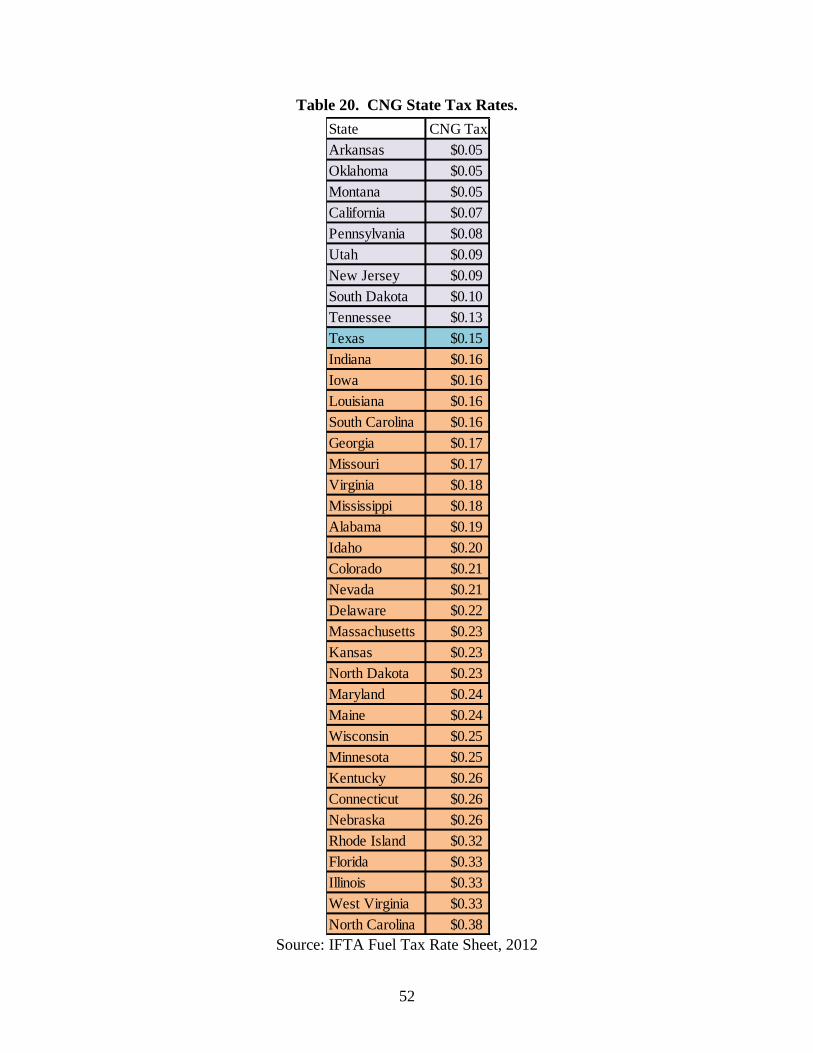
52

Table 20. CNG State Tax Rates.

Source: IFTA Fuel Tax Rate Sheet, 2012

State CNG Tax

Arkansas $0.05

Oklahoma $0.05

Montana $0.05

California $0.07

Pennsylvania $0.08

Utah $0.09

New Jersey $0.09

South Dakota $0.10

Tennessee $0.13

Texas $0.15

Indiana $0.16

Iowa $0.16

Louisiana $0.16

South Carolina $0.16

Georgia $0.17

Missouri $0.17

Virginia $0.18

Mississippi $0.18

Alabama $0.19

Idaho $0.20

Colorado $0.21

Nevada $0.21

Delaware $0.22

Massachusetts $0.23

Kansas $0.23

North Dakota $0.23

Maryland $0.24

Maine $0.24

Wisconsin $0.25

Minnesota $0.25

Kentucky $0.26

Connecticut $0.26

Nebraska $0.26

Rhode Island $0.32

Florida $0.33

Illinois $0.33

West Virginia $0.33

North Carolina $0.38

53

Figure 25. Annual Gasoline Consumption Historical Data.

Figure 26. Projected Texas Population.

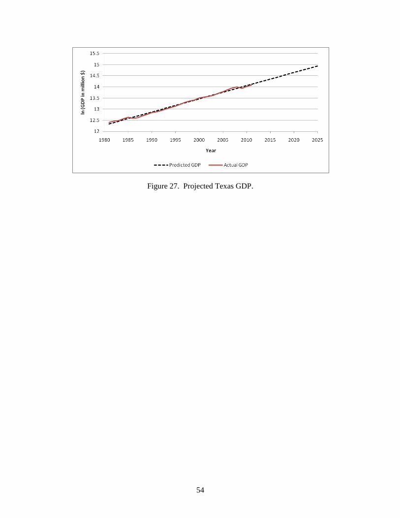
54

Figure 27. Projected Texas GDP.

EVALUATION OF POTENTIAL IMPACTS OF ALTERNATIVE...

Documents

Transcript of EVALUATION OF POTENTIAL IMPACTS OF ALTERNATIVE...