Evaluating the relative operational efficiency of large … · data envelopment analysis D. I....

Evaluating the relative operational efficiency of large-scale computer networks: an approach via data envelopment analysis

D. I. Giokas and G. C. Pentzaropoulos

Department of Economics, University of Athens, Athens, Greece

The objective of the present study was the development of a methodology to be used as an aid in decision making for the attainment of optimum operational eficiency in large-scale computer communications networks. The above methodology is realized in two stages. In the first stage, a queueing model (M/M/I/K) of a typical network is developed, and analytical results for the main performance indicators are obtained. The results are used, in the second stage, as a starting point for the application of a data envelopment analysis (DEA) procedure to obtain characteristics of network operational efficiency. Emphasis is placed on suggestions for improving the efficiency level of (relatively) inefficient nodes: numerical examples are also provided to illustrate the applicability of various options. Finally, possible routes for achieving a higher level of overah network efficiency are discussed, within the context of a performance tuning procedure, which are aimed at reducing the effects of performance bottlenecks.

Keywords: computer networks, queueing theory, operational efficiency, data envefopment analysis

1. Introduction

The primary role of a large-scale computer network is to distribute all available resources among its user community fairly and efficiently. In an active user environment, requests for service appear at random intervals, and the workload thus generated may, at certain periods of time, drive the network away from its steady state. As a result, stability problems may arise, at least in some of the network’s regions, which may undermine its operating capability.’ It is therefore necessary to study the effects that a variable traffic pattern may have on the network’s performance and, whenever possible, to suggest options that would result in a more efficient operation. In this effort, several possibilities may be considered, which range from the upgrading of network nodes to the regulation of local traffic at certain points. Economies of scale could be achieved by adopting a step-wise approach through which the options available for operational improve- ments are measured against the cost of their implementation. In this paper we examine the problem of overall network efficiency through the study of the relative efficiency levels of its main constituent parts (i.e., the

Address reprint requests to Dr. G. C. Pentzaropoulos at the Department of Economics, University of Athens, 8 Pesmazoglou & Stadiou Str, 105 59 Athens, Greece.

Received 28 July 1994; revised 19 December 1994; accepted 16 January 1995

Appl. Math. Modelling 1995, Vol. 19, June 0 1995 by Elsevier Science Inc. 655 Avenue of the Americas, New York, NY 10010

processing nodes); this is done by means of queueing theory modelling and the implementation of operational research techniques, as explained below.

A network node may be thought of as a semi- autonomous processing unit that accepts inputs from its environment and, by utilizing its own resources, produces outputs according to rules implemented in the unit’s structural system. This implies that a certain degree of intelligence is accommodated in such a unit, and this in fact may be observed in many of today’s networking structures. The decisions that are made locally are expected to have an impact within a wider region and as such could make overall network performance change in time. Accordingly, the kind and level of output produced by each unit (node) characterize its efficiency as regards the processing of tasks. In the following analysis we assume that all participating units (nodes) work according to the same rules (homogeneous processing environment); therefore, the outcome of a certain decision depends only on different levels of workload as well as variable traffic patterns.

The efficiency of decision-making units (DMUs) has traditionally been measured by means of ratio analysis. Such an approach gives a great deal of information about a unit’s performance in a distributed system but it also has several shortcomings. First, each ratio is limited to only two factors, one input and one output, and it is difficult to accommodate situations where multiple outputs are produced using multiple inputs; then, to formulate a ratio, one has to use relative weights, which

0307-904x/95/.$10.00 SSDI 0307-904X(95)00010-H

Evaluating relative network operational efficiency: D. 1. Giokas and G. C. Pentzaropoulos

are not always available for all such units. Second, a unit may occupy the first position when compared with a certain ratio, while it may occupy the last position when compared with another ratio; as a result, relative weights for each ratio are needed when large sets of ratios are calculated. Third, ordering efficiency across many DMUs, for a given ratio, makes it difficult to explain the behavior of individual DMUs. If the unit with the largest value is efficient, how far below this value (cut-off point) another unit is also efficient is not easy to detect.

Data envelopment analysis (DEA) was originally introduced by Charnes et al.’ for assessing the relative efficiency of DMUs that utilize multiple incommensurate inputs to produce multiple incommensurate outputs. The technique is based on an efficiency concept proposed by Farrell some years ago.3 DEA is capable of overcoming most of the difficulties associated with ratio analysis, and it is, therefore, a useful complement of this type of analysis. With DEA, one can consider simultaneously the case of multiple inputs and outputs to gain an overall evaluation of a unit’s efficiency, without the need to calculate relative weights. Using as a reference the so-called peer group members, this technique measures existing inefficiencies and suggests the adjustments needed (input reduction and/or output augmentation) that could make an inefficient unit efficient. This is done on a quantitative basis, by reallocating available resources among the DMUs being evaluated in order to improve overall efficiency. The data used in a DEA approach (inputs and outputs) may be measured or estimated in their natural physical units, without the need for a unified measurements environment. In fact, DEA may objectively rank the available units by their efficiency outcomes, without introducing an (arbitrary) cut-off point that separates efficient and inefficient units. In that respect, DEA measures efficiency by making comparisons among the whole spectrum of the available units, thus avoiding comparisons that are based on an average relationship that simply reflects a mixture of efficient and inefficient behavior.

The flexibility and versatility of DEA has been demonstrated in numerous applications since its first appearance in 1978. Environments evaluated include schools4 and universities,5 hospitals,6V7 insurance offices,* as well as branches in a distributed banking environment.9-‘3 The significant advantages that DEA offers have not, to our knowledge, been utilized in the performance management of computer networks (either large-scale or local ones). In this study we combine analytical modelling techniques from queueing theory with the predictive capabilities of DEA to obtain, in the first instance, a characterization of the operational efficiency of large-scale computer networks. Then we examine in more detail the reasons that could make a certain node exhibit suboptimal performance, when compared with other more efficient network nodes. Finally, we suggest possible alternatives for improving network node efficiency and show how such options may be applied in a typical situation. These options aim at reducing the effects of performance bottlenecks, thereby contributing to a better flow of information.

364 Appl. Math. Modelling, 1995, Vol. 19, June

2. Queueing network modelling

The general network topology includes N nodes, where N + 1 and an integer, as well as the necessary links between the nodes. For such a network, we define a virtual path to be a series of links that connect a specified number of nodes; moreover, an end-to-end virtual path has a source and a sink that are both located at the boundary of the network topology. As a matter of notation z,(, i, j,k,, , N1 represents an end-to-end virtual path which extends from node 1 (source) to node N (destination) also including some intermediate nodes like i, j, k, etc.

2.1 Network operational characteristics

Let us assume that Izi is the total flow into node i (measured in packets/set) from all adjacent nodes; this is the sum of all flow rates of the links that traverse node i and may be expressed in terms of the elements [rjk] of the network traffic matrix. The expression for Ai is, therefore:

li = i Yjk where j, k: Ljk~qiJ (1) 1 <j.k

that is, the link (channel) Ljk carries traffic converging to node i.

Each node in the network may be represented by the M/M/l/K queueing model, i.e., a system with exponential interarrival and service times and finite waiting room. These assumptions are common in many performance studies of computer communications networks14*15 (in which K is sometimes taken as infinite). Here, the presence of a finite K (but of variable value throughout the network) reflects the situation of nodes with memory constraints; such nodes are assumed to contain a limited number of buffers to accommodate the incoming messages (in the form of packets). The service discipline at node i is assumed to be in order of arrival, i.e., FCFS, and it is also assumed that l/pi represents the mean service time (in seconds) at the same node.

When the above network is formed by a series of exponential nodes (servers in queueing theory terms), i= 1,2,..., N, an analytical solution for the steady-state is available in closed-form expressions.‘6,‘7 A general measure of traffic intensity at node i is given by ri = ~i/~i. In the following analysis, we also use the measure &(w) = &l(p), where l(p) is the mean packet length (in Kbits), which denotes the mean workload (in Kbits/sec) placed on i. Also, the general expression of l/cLi may be adjusted to include network overheads, and this gives the following expression:

I/Pi(h) = (l/Pi) + (hRi) (2)

where h is the average network overhead, and Ri is a random number in the interval [0, l] which we have used to distribute h among the network nodes in a nonuniform way. From the above analysis we may now obtain:

ri(h) = Ai(w)lPi(h) = ~il(p){(IlPJ + (hRJ1 (3)

which is an adjusted traffic intensity expression. The values of lIpi and h may be calculated from known

Evaluating relative network operational efficiency: D. I. Giokas and G. C. Pentzaropoulos

network characteristics. Examples are given later in this section.

Of particular importance in this study is the estimation of the probability that all buffers of node i are full at a given time. For the nontrivial case, i.e., where li # pi, this probability is,

PK(~) = {Cl - ri(h)lri(hF)lC1 - ri(V+ ‘I (4)

with r,(h) as before. Because of space limitations (number of buffers available) the actual traffic entering node i, n,(e), will be:

k(e) = ni(w){ l - h&)1 = ni4P){ l - PAi)) (9 and the actual server (node i) utilization, pi, will be:

Pi = 4(eYPi(h) = ni(w){ 1 -Pdi))lPi(~) = (1 -Pfdi))ri(h) (6)

which represents the fraction of time node i is busy. One important measure in a network with limited

storage capacity is the number of packets that are turned away from node i, because all buffers are full at the time of arrival of the next packet. This may be expressed in percentage form by taking account of probability &I’) as follows:

Fi = loop,(i) (7)

and high values of Fi indicate a relative storage inefficiency of node i.

For nodes with significant memory constraints, and possibly large values of arrival rates, we may also expect large queue sizes, which again from the same model are estimated as:

Qi = {ri(h)lCl - r,(h)]) - {[(K + l)ri(h)“+‘]/(l - ri(h)K+l)) (8)

which as in the case of pK(i) in equation (4) is also true for the nontrivial case of ,$ # pi. Further, the mean waiting time r/r/;. is easily obtained by Little’s lawI and equation (5) as follows:

W = QJUe) (9)

and this is also measured in seconds. Since we prefer to use an expression of relative efficiency of node i, we introduce via equation (2) a normalized equivalent of & above as follows:

si = W/{(l/Pi) + (hRi)} (10) which we may call the stretch factor Si of node i. This is a useful measure that has been used to characterize processing efficiency in performance comparisons of various computer systems in a network” and shows how many times (over some required minimum time for service) a stream of packets may be delayed as a result of a large queue size. High values of this measure indicate a relative processing inefficiency of node i.

In summary, a network node i may be characterized by the following quantities:

(iI) Ai, total flow from all adjacent nodes (in packets/set);

(iZ) l/pi, mean service time (in seconds); (i3) Ki, memory capacity (in number of buffers

available); (ol) Pit mean node utilization (fraction between 0 and 1); (oJ Fi, packets turned away (%); (oJ Si, mean stretch factor (real number above 1).

In the context of DEA (iI), (iJ, and (Q (inherent measures) are the “input” parameters and (ol), (oJ, and (03) (productivity measures) are the “output” parameters. This definition is not unique but it is considered appropriate for our purposes.

2.2 Example of large-scale computer network

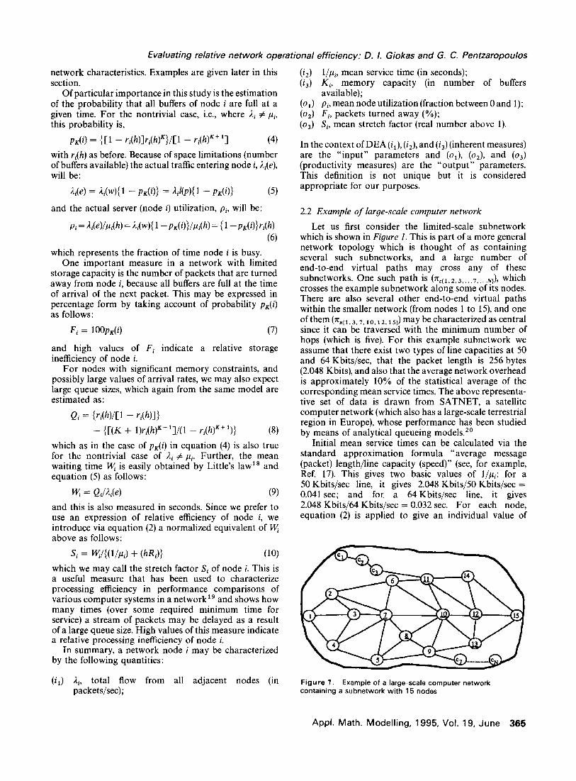
Let us first consider the limited-scale subnetwork which is shown in Figure 1. This is part of a more general network topology which is thought of as containing several such subnetworks, and a large number of end-to-end virtual paths may cross any of these subnetworks. One such path is (7~,(~,~, 3,, .7,, &, which crosses the example subnetwork along some of its nodes. There are also several other end-to-end virtual paths within the smaller network (from nodes 1 to 15), and one ofthem(~,~1,3,7,10,12,15) ) may be characterized as central since it can be traversed with the minimum number of hops (which is five). For this example subnetwork we assume that there exist two types of line capacities at 50 and 64 Kbits/sec, that the packet length is 256 bytes (2.048 Kbits), and also that the average network overhead is approximately 10% of the statistical average of the corresponding mean service times. The above representa- tive set of data is drawn from SATNET, a satellite computer network (which also has a large-scale terrestrial region in Europe), whose performance has been studied by means of analytical queueing models.*’

Initial mean service times can be calculated via the standard approximation formula “average message (packet) length/line capacity (speed)” (see, for example, Ref. 17). This gives two basic values of l/pi: for a 50 Kbits/sec line, it gives 2.048 Kbits/SO Kbits/sec = 0.041 set; and for. a 64 Kbits/sec line, it gives 2.048 Kbits/64 Kbits/sec = 0.032 sec. For each node, equation (2) is applied to give an individual value of

Figure 1. Example of a large-scale computer network containing a subnetwork with 15 nodes

Appl. Math. Modelling, 1995, Vol. 19, June 365


Table 1. Input/output performance parameters used for DEA

Inputs outputs

Node 1, K, 14 4 PI 6 s

Nl 7 10 24.390 0.590 0.213 2.393 N2 6 6 22.727 0.534 1.163 2.023 N3 10 7 23.256 0.815 7.790 3.511 N4 9 9 22.727 0.783 3.237 3.671 N5 9 7 22.727 0.772 5.559 3.219 N6 8 7 31.250 0.524 0.539 2.035 N7 11 11 30.303 0.734 0.987 3.440 N8 10 8 31.250 0.655 1.296 2.659 N9 8 8 28.571 0.566 0.475 2.230 NIO 14 15 30.303 0.903 3.716 6.830 Nil 10 10 29.412 0.686 0.783 2.984 N12 13 9 30.303 0.834 5.281 4.170 N13 12 10 28.571 0.825 3.757 4.280 N14 9 6 23.256 0.744 6.495 2.854 N15 11 12 23.256 0.904 6.048 6.044

l/pi(h) which, because of the presence of h, also includes network overheads. The inverse expressions of these values, i.e., pi(h), give the corresponding mean service rate values. With these assumptions under consideration, we may assign some typical values of input flows (&) and buffer sizes (Ki) for the 15 nodes and then obtain estimates for pi, F, and Si from equations (6), (7), and (10) respectively. The results of this analysis are summarized in Table 1; further, this input/output table is used for the DEA modelling procedure that follows.

3. Data envelopment analysis

The relative efficiency of a node (DMU in DEA terminology) may be defined as the ratio of the weighted sum of its outputs to the weighted sum of its inputs; the weights are determined so as to maximize the efficiency rating H, of the kth node being evaluated. Various mathematical forms of the original modelling scheme have appeared in the literature,21-23 which reflect situations where a particular DEA application was considered as more appropriate.

3.1 Overall modelling approach

The formulation used in this study is based on the so-called CCR model introduced by Charnes, Cooper, and Rhodes,’ and it is as follows:

Maximize H, = i u, . y,, f vi’~ik (Model A) I.=1 I i=l

(11) subject to

=;: U,’ Yrj

I

~ Vi. Xij I 1 ci = 1, 2,. . . ) N) (12)

r=l i=l

Up, Vi 2 E (i=1,2 ,..., m;r=l,2 ,..., s) (13)

where H, is the relative efficiency of the kth node; k is the node being assessed; N is the number of nodes; r

is the number of outputs, r = 1,2,. . . , s; i is the number of inputs, i = 1,2,. . . , m; Y,~ are the observed amounts of output r from nodej = 1,2,. . . , N; xij are the observed amounts of input i to node j = 1,2,. . . , N; E is a small positive number to ensure that all inputs and outputs have at least some weighting in the efficiency measure; and vi, u, are virtual multipliers (the weights to be determined) for input i and output r, respectively.

The above fractional programming model may be converted into a linear programming (LP) formz*22 so that the methods of LP can be applied. The equivalent DEA model can, thus, be stated as follows:

Maximize H, = i u,. y,, r=1

subject to

(Model B) (14)

it, Vi ’ Xik = 1 (15)

s

C U,'Y*j - ~ Vi' Xij IO o’= 1,2,..., N) (16) r=t i=l

u,, Vi 2 E (i = 1, 2,. . . , m; r = 1, 2,. . . , s) (17)

This model is run repetitively, with each unit node in the objective function, so as to derive an efficiency rating for all nodes. Thus, for each node, the observations from the outputs (y,j) and inputs (Xij) are used to estimate the respective coefficients (u, and vi) that maximize the objective function. In this study, because of the particular choice of the input/output parameters, it was thought better to formulate the dual model of B, Model C henceforth, which is as follows:

Minimize Z, - .@r s, + $i si) (Model C) (18)

subject to

f ‘pjY,j - y,k - S, = 0 (r = 1, 2,. . . , S) (19)

j=l

zkxik - ~ 'pjXij - Si = 0 (i = 1, 2,. . . , m) j=l

(20) Cpj, %, SC 2 O

(j=l,2 ,..., N;r=l,2 ,..., s;i=l,2 ,..., m) (21)

Z, unrestricted in sign

where ‘pj are the dual variables corresponding to constraints (16); s,, si are the slack variables corresponding to constraints (17); and Zk is the “efficiency” variable corresponding to constraints (15). The kth node is efficient if s,, si are equal to zero and Z, is equal to one. If the kth node is relatively inefficient, it must use less of each input by a quantity equal to:

z, * Xik - si

and increase output by

(22)

Yrk+ % (23)



Table 2. Overall network performance as characterized by node efficiency

Slacks

Node

Nl N2 N3 N4 N5 N6 N7 N8 N9 NIO Nil N12 N13 N14 N15

DEA Efficiency efficiency reference

score set

1.000 Nl 1.000 N2 1.000 N3 1 .ooo N4 1.000 N5 1.000 N6 0.975 Nl, N2, N4 0.951 N2, N6, N9 1.000 N9 0.867 Nl, N4 0.989 Nl, N2, N9 0.875 N2, N5, N14 0.899 N2, N4, N5 1 .ooo N14 1.000 N15

A,

2.186 1.706

1.757 1.835 1.706 1.303

Inputs

Ki

0.000 0.000

2.601 0.000

Pi(h) Pi

0.000 0.000

outputs

F,

0.000

si

0.467 0.166 0.000 2.599 0.283 0.752 0.621

in order to become efficient. With this set of targets, input enhancement is emphasized, as the main changes are to be in the input levels. (If preference is given to output enhancement, similar formulas to (22) and (23) may be derived.)

3.2 Numerical results for example network

The application of Model C requires that the more the outputs produced the better the efficiency. However, in the case of Fi and Si the opposite is true; for this reason, we reverse the sign of the corresponding constraints in equation (19).

Model C developed above provides several analytical interpretations which refer to: (a) the identification of the relative efficient and inefficient nodes, (b) the relative efficiency scores, (c) the peer groups (efficiency reference sets), and (d) the changes in the inputs and outputs for all relatively inefficient nodes that are necessary to make them efficient.

The results in Table 2 indicate that 6 nodes (N7, N8, NlO, Nil, N12, and N13) of the subnetwork in Figure I are relatively inefficient as they have an efficiency score of less than 1; for these nodes their respective numbers in the circles are underlined. Inefficiency reflects the proportion of the inputs (resources) a node should be using in principle, in order to secure its output levels, if it is to be efficient in comparison with other nodes. The analysis has identified a combination of one or more efficient nodes (the efficiency reference set) that can be used to secure the output levels of an inefficient node by using a proportion of its inputs equal to its efficiency score. As an example, node NlO is about 87% efficient compared with nodes Nl and N4; node N12 is also about 87% efficient but when compared with nodes N2, N5, and N14. Generally, this means that both NlO and N12 could reduce the inputs (resources) they utilize by

approximately 13% without having to reduce their outputs. Further, it can also be observed (from Table 2) that only seven nodes (Nl, N2, N4, N5, N6, N9, and N14) consistently appear in the peer groups (reference sets), implying that these nodes are the efficient ones. Nodes N3 and N15 are also considered as efficient, despite the fact that they do not appear in the reference sets of Table 2. We assume that these nodes have a distinctly different profile as regards their input/output variables.

The efficiency scores may also be interpreted in terms of output maximization. Hence, the performance of inefficient nodes may be improved either by increasing outputs (output enhancement is emphasized) or by cutting inputs (input reduction is emphasized) or by cutting inputs and increasing outputs simultaneously. There are infinite combinations of input-output levels that would make a relatively inefficient node efficient. To show a detailed node analysis, we next focus on node N12, which is identified as inefficient with Ii, = 0.875, compared with nodes N2, N5, and N14 (its efficiency reference set).

Let us clarify that, for each inefficient node (e.g., N12), DEA first identifies its corresponding efficiency reference set. This is a set of relatively efficient nodes to which the current inefficient node has been most directly compared in calculating its efficiency score. The above reference set, which is a convex combination of the actual inputs and outputs with respect to (e.g., N2, N5, N14), also identifies a “composite node” which is the hypothetical efficient node that we would like the nonefficient node N12 to become. This information is a result of DEA. Therefore, the amounts of inputs that node N12 should have been using are given by application of formula (22) as follows:

X, = 13 *0.875 - 1.706 = 9.67 (24) X, = 9 * 0.875 - 0.0 = 7.87 (25) X,, = 30.3 * 0.875 - 0.0 = 26.51 (26)

Appl. Math. Modelling, 1995, Vol. 19, June 367

Evaluating relative network operational efficiency: D.

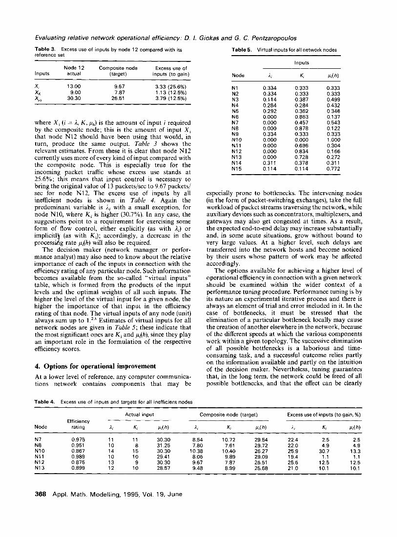
Table 3. Excess use of inputs by node 12 compared with its reference set

Inputs

x;

xK

xWl

Node 12 actual

13.00

9.00 30.30

Composite node (target)

9.67 7.87

26.51

Excess use of inputs (to gain)

3.33 (25.6%) 1 .13 (12.5%) 3.79 (12.5%)

where Xi (i = 2, K, p,,) is the amount of input i required by the composite node; this is the amount of input Xi that node N12 should have been using that would, in turn, produce the same output. Table 3 shows the relevant estimates. From these it is clear that node N12 currently uses more of every kind of input compared with the composite node. This is especially true for the incoming packet traffic whose excess use stands at 25.6%; this means that input control is necessary to bring the original value of 13 packets/set to 9.67 packets/ set for node N12. The excess use of inputs by all inefficient nodes is shown in Table 4. Again the predominant variable is J.; with a small exception, for node NlO, where Ki is higher (30.7%). In any case, the suggestions point to a requirement for exercising some form of flow control, either explicitly (as with &) or implicit1 (as with K,); accordingly, a decrease in the

J process’ g rate pi(h) will also be required. The decision maker (network manager or perfor-

mance analyst) may also need to know about the relative importance of each of the inputs in connection with the efficiency rating of any particular node. Such information becomes available from the so-called “virtual inputs” table, which is formed from the products of the input levels and the optimal weights of all such inputs. The higher the level of the virtual input for a given node, the higher the importance of that input in the efficiency rating of that node. The virtual inputs of any node (unit) always sum up to 1. 23 Estimates of virtual inputs for all network nodes are given in Table 5; these indicate that the most significant ones are Ki and pi(h), since they play an important role in the formulation of the respective efficiency scores.

4. Options for operational improvement

At a lower level of reference, any computer communications network contains components that may be

Table 4. Excess use of inputs and targets for all inefficient nodes

‘. Giokas and G. C. Pentzaropoulos

Table 5. Virtual inputs for all network nodes

Inputs

Node A; K, vi(h)

Nl 0.334 0.333 0.333 N2 0.334 0.333 0.333 N3 0.114 0.387 0.499 N4 0.284 0.284 0.432 N5 0.292 0.362 0.346 N6 0.000 0.863 0.137 N7 0.000 0.457 0.543 N8 0.000 0.878 0.122 N9 0.334 0.333 0.333 NIO 0.000 0.000 1.000 Nil 0.000 0.696 0.304 N12 0.000 0.834 0.166 N13 0.000 0.728 0.272 N14 0.311 0.378 0.311 N15 0.114 0.114 0.772

especially prone to bottlenecks. The intervening nodes (in the form of packet-switching exchanges), take the full workload of packet streams traversing the network, while auxiliary devices such as concentrators, multiplexers, and gateways may also get congested at times. As a result, the expected end-to-end delay may increase substantially and, in some acute situations, grow without bound to very large values. At a higher level, such delays are transferred into the network hosts and become noticed by their users whose pattern of work may be affected accordingly.

The options available for achieving a higher level of operational efficiency in connection with a given network should be examined within the wider context of a performance tuning procedure. Performance tuning is by its nature an experimental iterative process and there is always an element of trial and error included in it. In the case of bottlenecks, it must be stressed that the elimination of a particular bottleneck locally may cause the creation of another elsewhere in the network, because of the different speeds at which the various components work within a given topology. The successive elimination of all possible bottlenecks is a laborious and time- consuming task, and a successful outcome relies partly on the information available and partly on the intuition of the decision maker. Nevertheless, tuning guarantees that, in the long term, the network could be freed of all possible bottlenecks, and that the effect can be clearly

Node Efficiency

rating

Actual input Composite node (target) Excess use of inputs (to gain, %)

K, Pi(h) 1 I, K p,(h) A, K, p,(h)

N7 0.975 11 11 30.30 8.54 10.72 29.54 22.4 2.5 2.5 N8 0.951 10 8 31.25 7.80 7.61 29.72 22.0 4.9 4.9 NIO 0.867 14 15 30.30 10.38 10.40 26.27 25.9 30.7 13.3 Nil 0.989 10 10 29.41 8.06 9.89 29.09 19.4 1 .l 1 .l N12 0.875 13 9 30.30 9.67 7.87 26.51 25.6 12.5 12.5 N13 0.899 12 10 28.57 9.48 8.99 25.68 21 .o 10.1 10.1



seen in the values of any suitable performance indices (e.g., end-to-end delay or received throughput).

From the previous analysis, several possibilities for improving overall network efficiency have been shown to exist. The search for options, on the part of the decision-maker, could be directed toward the following routes:

(4

0.4

(4

(4

(4

The identification of all network nodes that may constitute bottlenecks; these have an efficiency rating of less than 1 and may be considered as suboptimal in relation to the efficient nodes; The identification of optimal end-to-end paths, i.e., those that connect optimal nodes, if any such paths exist; The estimation of the smallest number of hops that are needed to traverse the network along all of its optimal paths, if any such number exists; The identification of the node(s) with the lowest efficiency score(s); and The identification of possible bottlenecks around any central node, i.e., one that carries traffic from source to sink along a central circuit.

The above procedures should aim at reallocating existing capacities to the estimated volume and pattern of flow within a given network topology.

Returning to the example subnetwork of Figure 1, we first note that there are six suboptimal nodes (N7, N8, NlO, Nil, N12, Ni3) and that there are no optimal end-to-end paths present, since the region formed by nodes Nil, N12, and N13 is currently blocking (optimal) entrance to the sink node (N15). As a consequence, there is at present no way to traverse the network optimally (irrespective of a possible number of hops). It also happens that the node with the lowest efficiency rating (NlO) is central, which points to a possible bottleneck located in middle of this subnetwork structure. Finally, two more central nodes (N7 and N12) are also suboptimal and therefore suspected to form bottlenecks there. From the suggestions that have been derived in the previous sections, one may give a priority to those that could, in some sense, help free nodes that carry a sizeable amount of traffic (e.g., NlO, N12, N13) but not necessarily all of them at the same time. The first candidate might be the node with the lowest efficiency rating (again, NlO), and the search could subsequently be directed as to:

(1) Create at least one optimal end-to-end path (with any number of hops, at first);

(2) Successively eliminate all bottlenecks along a central path on an end-to-end basis; and

(3) Estimate the cost of the implementation of any other feasible actions and consider alternative ones (equivalent in terms of efficiency) if some are too costly to implement.

By referring to the example subnetwork once again, we note that a peripheral path such as rrn(1,2,6,11,14,15) could be made optimal if node Nil is made efficient.

From Table 4, we note that this is achieved if 1, 1, K 1 1, and prr(h) are reduced by 19.4, 1.1, and l.l%, respectively. This means that it is necessary to shift 19.4% of the incoming traffic away from node Nil, perhaps to a less congested part of the network, and to make some rather minor adjustments in the node’s memory and processing rate. For the central path rc,(, 3 ,, i0 r2, 15) to become optimal, a series of actions is required involving nodes N7, NlO, and N12. The suggestions given in Table 4 call for some major adjustments toward controlling the input flow at node N7 and substantial adjustments across all variables for nodes NlO and N12.

At this point it should be noted that the type of action adopted in a real situation will largely depend on specific priorities; this is an important constraint as it is known from experience that the implementation of certain types of action is often outside managerial control and sometimes prohibitively expensive, especially in a large-scale capacity planning exercise. A useful option in such cases would be to estimate the level of improvement that might be achieved by the implementation of a series of limited-scale modifications, which could be done selectively rather than fully. In such cases, the result sought is not 100% optimality for all inefficient network nodes, but rather an acceptable improvement on the observed efficiency ratings. The relative significance of virtual input values, as they appear in Table 5, could be used as a guide toward the achievement of near-optimal ratings; thus, Ki should be selected for nodes N8, N12, and N13, pi(h) for node NlO, and both Ki and pi(h) for nodes N7 and Nil. The results from the above selection are summarized in Table 6. We note that the level of improvement is significant for all six inefficient network nodes and this is especially true for node NlO (central), which was from the beginning the one with the lowest efficiency score. We should therefore expect an efficiency level of no less than 97% for all network nodes.

For the special problem of flow balancing with reference to the network received (or end-to-end) throughput, more elaborate techniques such as linear goal programming may be employed, in which cost is an integral part of the overall optimization procedure.24 If the complete network is too complex to be considered as a single entity, the decision maker may wish to partition it in a number of smaller subnetworks, of manageable proportions, and then apply the previous analysis. Each subnetwork could be studied separately, and the results could be applied to the entire network using standard decomposition/aggregation techniquesz5

Table 6. Improvement for the limited-scale option

Efficiency Efficiency Improvement Node rating (old) rating (new) W)

N7 0.975 0.9999 2.55 N8 0.951 0.9988 5.03 NlO 0.867 0.9998 15.32 Nil 0.989 0.9992 1.03 N12 0.875 0.9739 11.30 N13 0.899 0.9693 7.82

APPI. Math. Modelling, 1995, Vol. 19, June 369


Care should be taken to preserve the relative identity of each isolated subnetwork for the aggregation exercise to be applicable. In the case where the object network contains a satellite segment (as in the case of SATNET mentioned in the example), the partitioning may be applied at first to give a terrestrial and a satellite environment; the results may subsequently be combined to give estimates of overall network efficiency.

References

1

2

Fontecha, F., Wang, X., Onozato, Y. and Noguchi, S. Structural stability in communication networks. Stochastic Analysis of Computer and Communication Systems, ed. H. Takagi, IFIP Publication, North-Holland, Amsterdam, 1990, pp. 767-805 Charnes, A., Cooper, W. W. and Rhodes, E. Measuring the efficiency of decision-making units. Eur. J. Opl. Res. 1978, 2, 4299444

3

4

Farrell, M. J. The measurement of productive efficiency. J. Roy. Stat. Sot. Series A 1957, 120(3), 2533281 Bessent, A., Bessent, W., Kennington, J. and Reagan, B. An application of mathematical programming to assess productivity in the Houston independent school district. Mgmt. Sci. 1982, 28(12), 1355-1367 Beasly, J. E. Comparing university departments. Omega Int. J. Mgmr. Sci. 1990, 18(2), 171-183 Morey, R. C., Fine, D. J. and Loree, S. W. Comparing the allocative efficiencies of hospitals. Omega Int. J. Mgmt. Sci. 1990, 18(l), 71-83 Sherman, H. D. Hospital efficiency measurement and evaluation. Medical Care 1984, 22(10), 922-938 Bjurek, H., Hjalmarsson, L. and Forsund, F. R. Deterministic parametric and non-parametric estimation of efficiency in service production: A comparison. J. Econometrics 1990,46(1/2), 213-227 Berg, S. A., Forsund, F. R. and Jansen, E. S. Bank output measurement and the construction of best practice frontiers. J. Producliv. Analysis 1991, 2, 127-142 Ferrier, G. and Lovell, C. Measuring cost efficiency in banking: Econometric and linear programming evidence. J. Economet. 1990,46(/2), 229-245 Giokas, D. Bank branch operating efficiency: A comparative application of DEA and the Loglinear Model. Omega. Inf. J. Mgmt. Sci. 1991, 19(6), 549-557 Sherman, H. D. and Gold, F. Bank branch operating efficiency: Evaluation with Data Envelopment Analysis. J. Bank. Finance 1985, 9, 297-315 Vassiloglou, M. and Giokas, D. A study of the relative efficiency of bank branches: An application of Data Envelopment Analysis. J. Opl. Res. Sot. 1990, 41, 591-597 Hayes, J. F. Modelling and Analysis of Computer Communications Nelworks. Plenum Press, New York, 1984 Daigle, J. N. Queueing Theory for Telecommunications. Addison- Wesley, Reading, MA, 1992 Kleinrock, L. Queueing Systems, Vol. 2: Computer Applications. Wiley, New York, 1976 Allen, A. 0. Probability, Statistics, and Queueing Theory with Computer Science Applications, Second Edition. Academic Press, London, 1990 Little, J. D. C. A proof of the queueing formula “I?, = IW”. Opns. Res. 1961,9, 3833387 Barney, G. C., Pentzaropoulos, G. C. and Swindells, W. Performance comparisons within a computer network of Prime systems. Proc. IEEE Melecon ‘83 (No A506), Athens, Greece 2426 May 1983 Pentzaropoulos, G. C. Steady-state and asymptotic performance of SATNET under variable packet flow conditions. Compuf. Commun. 1991, 14(3), 157-165 Seiford, L. M. and Thrall, R. M. Recent developments in DEA: The mathematical programming approach to frontier analysis. J. Economefrics 1990, 46(/2), 7-38 Banker, R. D., Charnes, A. and Cooper, W. W. Some models for estimating technical and scale inefficiencies in Data Envelopment Analysis. Mgmr. Sci. 1984, 30(9), 107881092 Boussotiane, A., Dyson, R. G. and Thanassoulis, E. Applied data envelopment analysis. Eur. J. Opl. Res. 1991, 52, 1-15 Pentzaropoulos, G. C. and Giokas, D. I. Cost- performance modelling and optimization of network flow balance via linear goal programming analysis. Comput. Commun. 1993, 16(10), 645-652 Courtois, P. J. Decomposability: Queueing and Computer Systems Applicaiions. Academic Press, New York, 1977

5. Conclusions

The objective of this study has been the development of a methodology for evaluating the operational efficiency of large-scale computer communications networks. This was made possible (to a certain degree) by the formulation of a two-stage analytical procedure. In the first stage, the object network was modelled as a typical store-and-forward queueing network with limited storage capacity (M/M/l/K), and results for the main performance indicators such as source (node) utilization and stretch factor were obtained in closed-form expressions. The input/output table of this analysis was subsequently used as the starting point for the application of a Data Envelopment Analysis (DEA) procedure, which occupied the second stage.

Using a typical network as an example, some numerical results were next obtained which illustrated the applicability of the method and its versatility in producing estimates that could form the basis of a subsequent decision-making process. Several tables were produced to show a complete characterization of network node efficiency, including estimates for trans- forming a currently inefficient node to an efficient one. The concept of “virtual inputs” table, which points out the relative importance of the variables chosen for the analysis, was used as a guide for establishing sensitivity areas that could be explored in the first instance. Possible routes for utilizing options for network operational improvement were also given, and these might prove useful in identifying and, whenever possible, eliminating performance bottlenecks.

The end result of an investigation into alternative solutions for obtaining better network efficiency should be the formulation of a suitable decision-making process that would finally lead to the most appropriate route, using the choices available. Some of the resulting actions may imply the need for financial commitments, especially during a network reconstruction or expansion phase; therefore, these should be measured against the cost of their implementation. After an examination of all available solutions, a decision could be reached on whether or not some particular type of action would be operationally useful and financially feasible in terms of the expected performance gains.

Acknowledgments

The authors would like to express their thanks to P. Germanou for providing help with programming and file management.

5

6

7

8

9

10

11

12

13

18

19

20

21

22

23

24

25


Evaluating the relative operational efficiency of large … · data envelopment analysis D. I....

Documents

Transcript of Evaluating the relative operational efficiency of large … · data envelopment analysis D. I....