
Data Envelopment Analysis.ppt
128
Data Envelopment Analysis Robert M. Hayes 2005
-
Upload
oluwadolapo-dolapo -
Category
Documents
-
view
207 -
download
9
Transcript of Data Envelopment Analysis.ppt

Data Envelopment Analysis
Robert M. Hayes2005

Overview
Introduction Data Envelopment Analysis DEA Models Extensions to include a priori Valuations Strengths and Weaknesses of DEA Implementation of DEA The Example of Libraries Annals of Operations Research 66 Annals of Operations Research 73

Introduction
Utility Functions Cost/Effectiveness Interpretation for Libraries

Utility Functions A fundamental requirement in applying operations research models is the
identification of a "utility function" which combines all variables relevant to a decision problem into a single variable which is to be optimized. Underlying the concept of a utility function is the view that it should represent the decision-maker's perceptions of the relative importance of the variables involved rather than being regarded as uniform across all decision-makers or externally imposed.
The problem, of course, is that the resulting utility functions may bear no relationship to each other and it is therefore difficult to make comparisons from one decision context to another. Indeed, not only may it not be possible to compare two different decision-makers but it may not be possible to compare the utility functions of a single decision-maker from one context to another.
Cost/Effectiveness
A traditional way to combine variables in a utility function is to use a cost/effectiveness ratio, called an "efficiency" measure. It measures utility by the "cost per unit produced". On the surface, that would appear to make comparison between two contexts possible by comparing the two cost/effectiveness ratios. The problem, though, is that two different decision-makers may place different emphases on the two variables.
Cost/Effectiveness It also must be recognized that effectiveness will usually entail
consideration of a number of products and services and costs a number of sources of costs. Cost/effectiveness measurement requires combining the sources of cost into a single measure of cost and the products and services into a single measure of effectiveness.
Again, the problem of different emphases of importance must be recognized. This is especially the case for the several measures of effectiveness. But it may also be the case with the several measure of costs, since some costs may be regarded as more important than others even though they may all be measured in dollars. When some costs cannot be measured in dollars, the problem is compounded.
Cost/Effectiveness
More generally, instead of costs and effectiveness, the variables may be identified as "input" and "output". The efficiency ratio is then no long characterized as cost/effectiveness but as "output/input", but the issues identified above are the same.

Interpretation for Libraries
This issue can be illustrated by evaluating library performance. Effectiveness here is the extent to which library services meet the expectations or goals set by the organization served. It is likely to be measured by several services which are the outputs of library operations—making a collection available for use, circulation or other uses of materials, answering of information questions, instructing and consulting.
Inputs are represented by acquisitions, staff, and space, to which evident costs can be assigned, but they are also represented by measures of the populations served.
Interpretation for Libraries
Efficiency measures the library’s ability to transform its inputs (resources and demands) into production of outputs (services). The objective in doing so is to optimize the balance between the level of outputs and the level of inputs. The success of the library, like that of other organizations, depends on its ability to behave both effectively and efficiently.
The issue at hand, then is how to combine the several measures of input and output into a single measure of efficiency. The method we will examine is that called "data envelopment analysis".
Data Envelopment Analysis
Data Envelopment Analysis (DEA) measures the relative efficiencies of organizations with multiple inputs and multiple outputs. The organizations are called the decision-making units, or DMUs.
DEA assigns weights to the inputs and outputs of a DMU that give it the best possible efficiency. It thus arrives at a weighting of the relative importance of the input and output variables that reflects the emphasis that appears to have been placed on them for that particular DMU.
At the same time, though, DEA then gives all the other DMUs the same weights and compares the resulting efficiencies with that for the DMU of focus.
Data Envelopment Analysis
If the focus DMU looks at least as good as any other DMU, it receives a maximum efficiency score. But if some other DMU looks better than the focus DMU, the weights having been calculated to be most favorable to the focus DMU, then it will receive an efficiency score less than maximum.
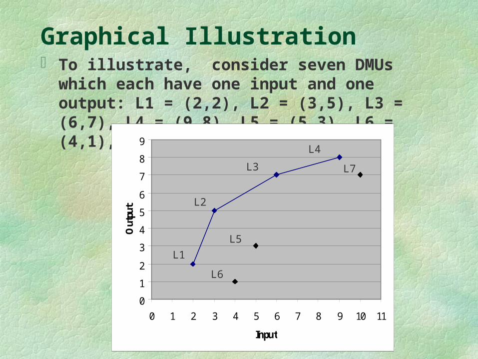
Graphical Illustration To illustrate, consider seven DMUs which each have
one input and one output: L1 = (2,2), L2 = (3,5), L3 = (6,7), L4 = (9,8), L5 = (5,3), L6 = (4,1), L7 = (10,7).
0
1
2
3
4
5
6
7
8
9
0 1 2 3 4 5 6 7 8 9 10 11
Input
Out
put
L1
L2
L3
L4
L5
L6
L7
Graphical Illustration
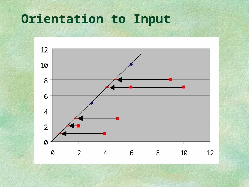
DEA identifies the units in the comparison set which lie at the top and to the left, as represented by L1, L2, L3, and L4. These units are called the efficient units, and the line connecting them is called the "envelopment surface" because it envelops all the cases.
DMUs L5 through L7 are not on the envelopment surface and thus are evaluated as inefficient by the DEA analysis. There are two ways to explain their weakness. One is to say that, for example, L5 could perhaps produce as much output as it does, but with less input (comparing with L1 and L2); the other is to say it could produce more output with the same input (comparing with L2 and L3).
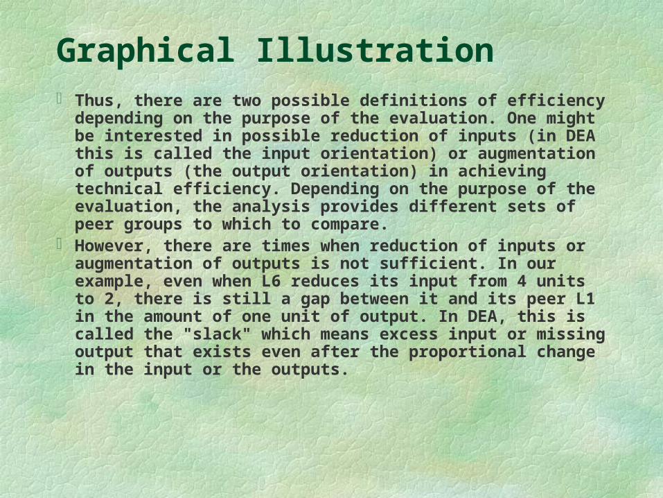
Graphical Illustration Thus, there are two possible definitions of efficiency depending
on the purpose of the evaluation. One might be interested in possible reduction of inputs (in DEA this is called the input orientation) or augmentation of outputs (the output orientation) in achieving technical efficiency. Depending on the purpose of the evaluation, the analysis provides different sets of peer groups to which to compare.
However, there are times when reduction of inputs or augmentation of outputs is not sufficient. In our example, even when L6 reduces its input from 4 units to 2, there is still a gap between it and its peer L1 in the amount of one unit of output. In DEA, this is called the "slack" which means excess input or missing output that exists even after the proportional change in the input or the outputs.
Graphical Illustration
This example will be used to illustrate the several forms that the DEA model can take.
In each case, the results presented are based on the implementation of DEA that will be discussed later in this presentation. It is an Excel spreadsheet using the add-in Solver capability.
The spreadsheet is identical for all of the forms, but the application of Solver differs in the target optimized and in the values to be varied, so for each form the target and the values to be varied will be identified.
DEA Models
The Basic EDA Concept Variations of DEA Formulation Formulation: Primal or Dual Orientation: Input or Output Returns to Scale: Fixed or Variable
The Basic EDA Concept
Assume that each DMU has values for a set of inputs and a set of outputs.
Choose non-negative weights to be applied to the inputs and outputs for a focus DMU so as to maximize the ratio of weighted outputs divided by weighted inputs
But do so subject to the condition that, if the same weights are applied to each of the DMUs (including the focus DMU), the corresponding ratios are not greater than 1
Do that for each DMU. The resulting value of the ratio for each DMU is its EDA
efficiency. It is 1 if the DMU is efficient and less than 1 if it is not.
Formulation
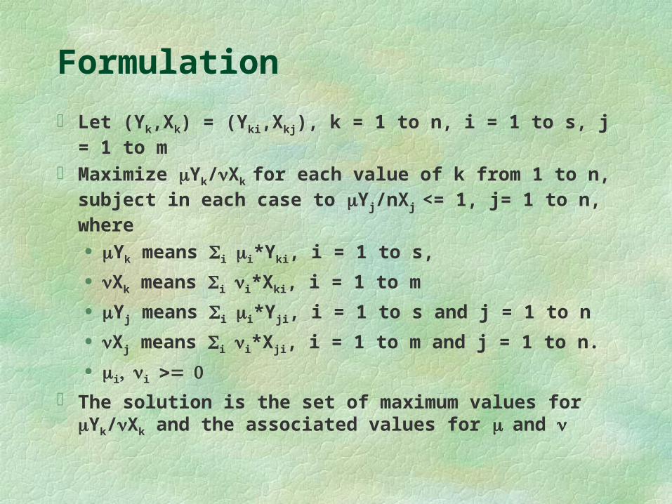
Let (Yk,Xk) = (Yki,Xkj), k = 1 to n, i = 1 to s, j = 1 to m
Maximize Yk/Xk for each value of k from 1 to n, subject in each case to Yj/nXj <= 1, j= 1 to n, where
Yk means ii*Yki, i = 1 to s,
Xk means ii*Xki, i = 1 to m
Yj means ii*Yji, i = 1 to s and j = 1 to n
Xj means ii*Xji, i = 1 to m and j = 1 to n.
ii The solution is the set of maximum values for Yk/Xk
and the associated values for and
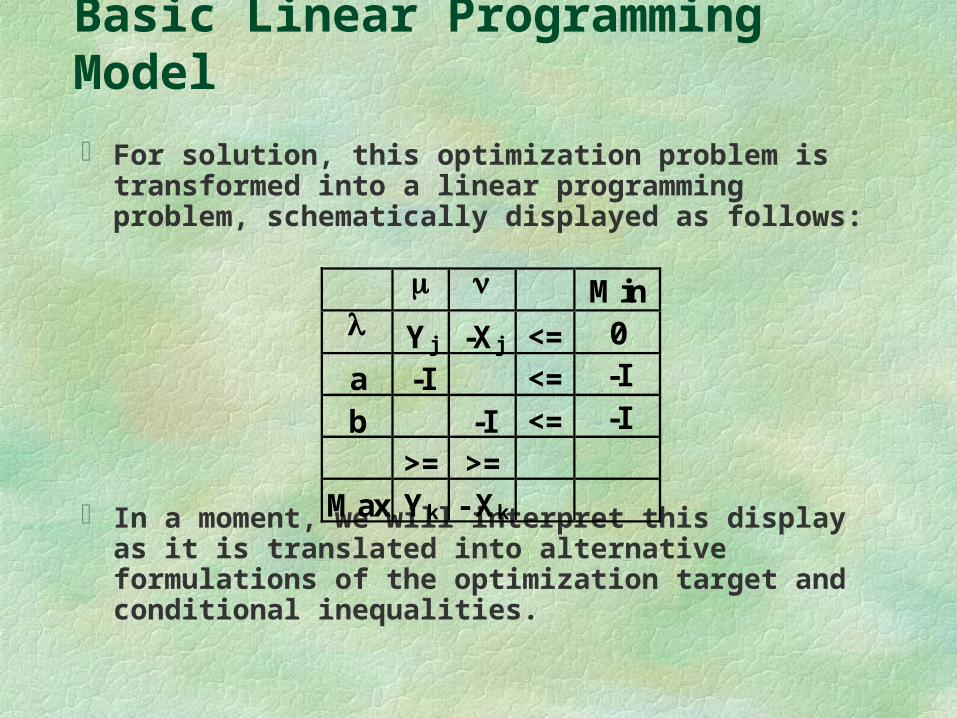
Basic Linear Programming Model
For solution, this optimization problem is transformed into a linear programming problem, schematically displayed as follows:
In a moment, we will interpret this display as it is translated into alternative formulations of the optimization target and conditional inequalities.
Min Yj -Xj <= 0
a -I <= -I
b -I <= -I
>= >=
Max Yk - Xk
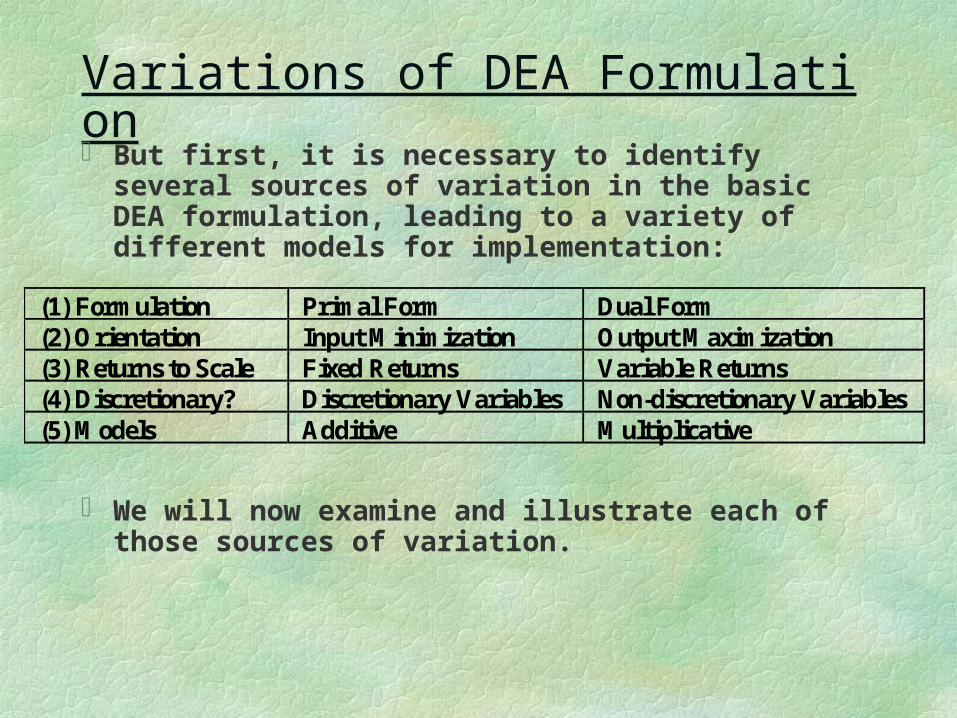
Variations of DEA Formulation But first, it is necessary to identify several sources of
variation in the basic DEA formulation, leading to a variety of different models for implementation:
We will now examine and illustrate each of those sources of variation.
(1) Formulation Primal Form Dual Form (2) Orientation Input Minimization Output Maximization (3) Returns to Scale Fixed Returns Variable Returns (4) Discretionary? Discretionary Variables Non-discretionary Variables (5) Models Additive Multiplicative
(1) Formulation: Primal or Dual
The first source of variation is interpretation of the display for the linear programming model.
One interpretation, called the Primal, treats the rows of the display as representing the model.
The other interpretation, called the Dual, treats the columns as representing the model.
Let’s examine each of those in turn.
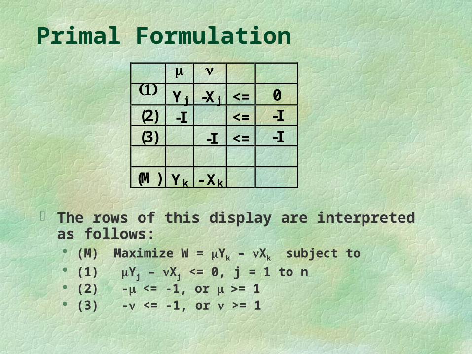
Primal Formulation
The rows of this display are interpreted as follows: (M) Maximize W = Yk – Xk subject to (1) Yj – Xj <= 0, j = 1 to n (2) -<= -1, or = 1 (3) - <= -1, or >= 1
Yj -Xj <= 0 (2) -I <= -I (3) -I <= -I
(M) Yk - Xk
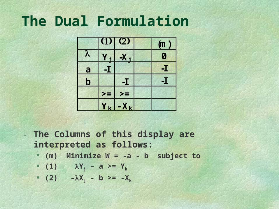
The Dual Formulation
The Columns of this display are interpreted as follows: (m) Minimize W = -a - b subject to (1) Yj – a >= Yk
(2) –Xj - b >= -Xk
(m) Yj -Xj 0
a -I -I
b -I -I
>= >=
Yk - Xk
The Choice of Formulation
Since the results from the two formulation are equal, though expressed differently, the choice between them is based on computational efficiency or, perhaps, ease of interpretation.
The Dual form is more efficient in computation if the number of DMUs is large compared to the number of input and output variables. Note that the Primal form entails n conditions (n being the number of DMUs) which, in the Dual form, are replaced by just m + s conditions (m being the number of input variables and s, the number of output variables)
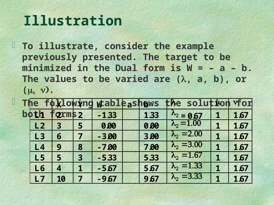
Illustration
To illustrate, consider the example previously presented. The target to be minimized in the Dual form is W = – a – b. The values to be varied are (, a, b), or ( .
The following table shows the solution for both forms: X Y W a b L1 2 2 - 1.33 1.33 = 0.67 1 1.67 L2 3 5 0.00 0.00 1 1.67 L3 6 7 - 3.00 3.00 1 1.67 L4 9 8 - 7.00 7.00 1 1.67 L5 5 3 - 5.33 5.33 1 1.67 L6 4 1 - 5.67 5.67 1 1.67 L7 10 7 - 9.67 9.67 1 1.67
Illustration
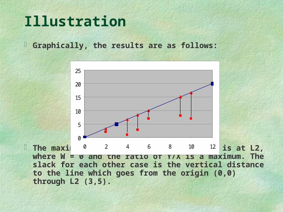
Graphically, the results are as follows:
The maximum value for W, over all cases, is at L2, where W = 0 and the ratio of Y/X is a maximum. The slack for each other case is the vertical distance to the line which goes from the origin (0,0) through L2 (3,5).
0
5
10
15
20
25
0 2 4 6 8 10 12
(2) Orientation: Input or Output
The second source of variation, orientation, provides the means for focusing on minimizing input or on maximizing output.
These represent two quite different objectives in making assessments of efficiency. Is the objective to be minimally expensive (e.g., to save money) or is it to be maximally effective?
Orientation to Input
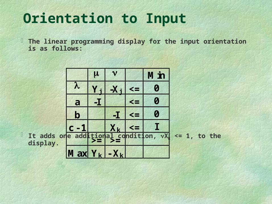
The linear programming display for the input orientation is as follows:
It adds one additional condition, Xk <= 1, to the display.
Min Yj -Xj <= 0
a -I <= 0
b -I <= 0
c - 1 Xk <= I
>= >=
Max Yk - Xk
Orientation to Input
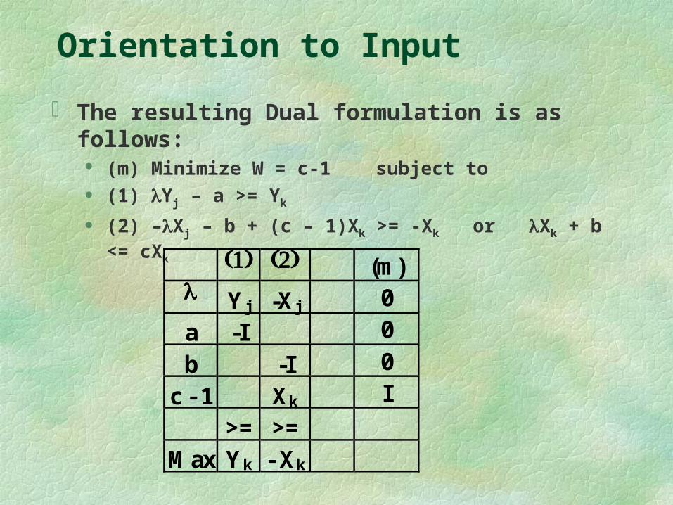
The resulting Dual formulation is as follows: (m) Minimize W = c-1 subject to (1) Yj – a >= Yk
(2) –Xj – b + (c – 1)Xk >= -Xk or Xk + b <= cXk
(m) Yj -Xj 0
a -I 0
b -I 0
c - 1 Xk I
>= >=
Max Yk - Xk

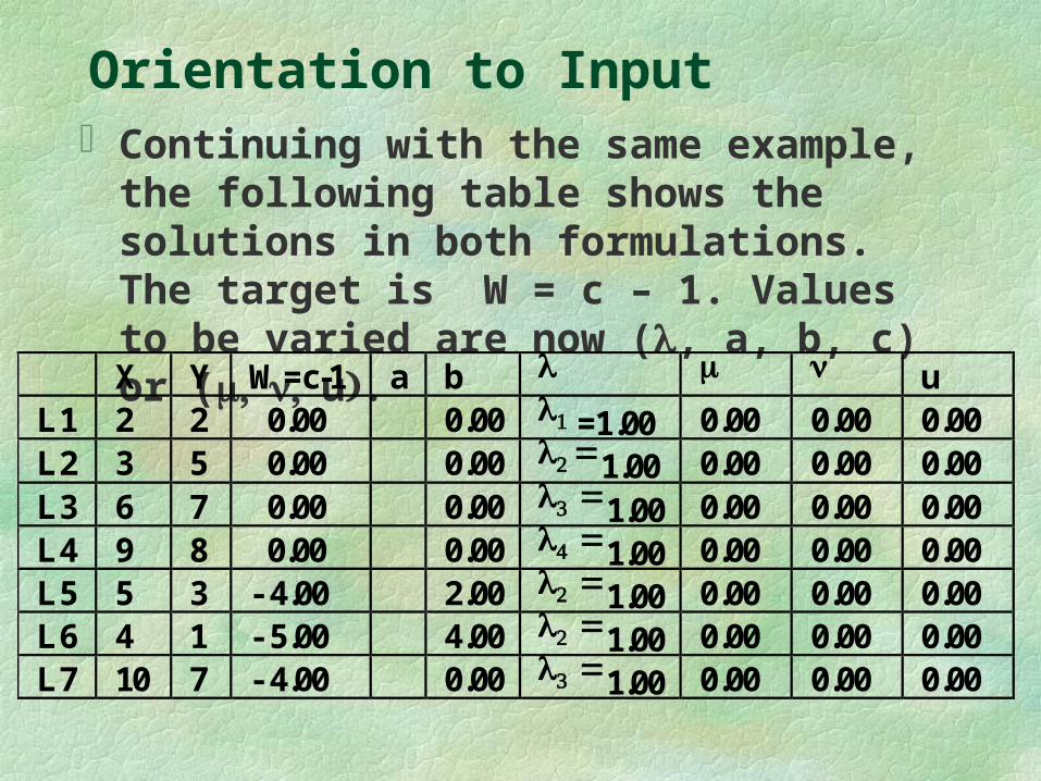
Orientation to Input Continuing with the same example, the following table shows the
solutions in both formulations. The target is W = c – 1. Values to be varied are now (, a, b, c) or ( and .
Note that L2 still dominates the solution, but the graph is now quite different,
X Y W=c-1 a b L1 2 2 - 0.40 = 0.40 0.30 0.50 L2 3 5 0.00 0.20 0.33 L3 6 7 - 0.30 0.10 0.17 L4 9 8 - 0.46 0.07 0.11 L5 5 3 - 0.64 0.12 0.20 L6 4 1 - 0.85 0.15 0.25 L7 10 7 - 0.58 0.06 0.10
Orientation to Input
0
2
4
6
8
10
12
0 2 4 6 8 10 12
Orientation to Output
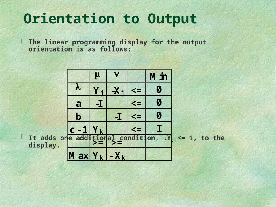
The linear programming display for the output orientation is as follows:
It adds one additional condition, Yk <= 1, to the display.
Min Yj -Xj <= 0
a -I <= 0
b -I <= 0
c - 1 Yk <= I
>= >=
Max Yk - Xk
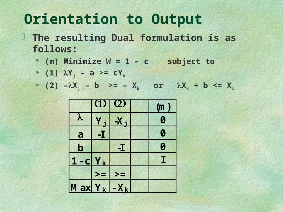
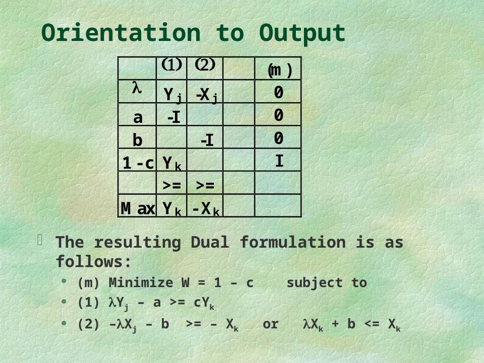
Orientation to Output The resulting Dual formulation is as follows:
(m) Minimize W = 1 – c subject to (1) Yj – a >= cYk
(2) –Xj – b >= – Xk or Xk + b <= Xk
(m) Yj -Xj 0
a -I 0
b -I 0
1 - c Yk I
>= >=
Max Yk - Xk
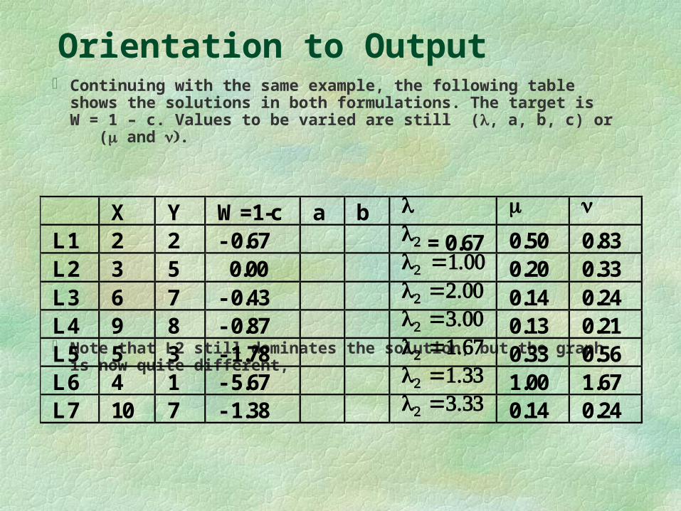
Orientation to Output Continuing with the same example, the following table shows the
solutions in both formulations. The target is W = 1 – c. Values to be varied are still (, a, b, c) or ( and .
Note that L2 still dominates the solution, but the graph is now quite different,
X Y W=1-c a b L1 2 2 - 0.67 = 0.67 0.50 0.83 L2 3 5 0.00 0.20 0.33 L3 6 7 - 0.43 0.14 0.24 L4 9 8 - 0.87 0.13 0.21 L5 5 3 - 1.78 0.33 0.56 L6 4 1 - 5.67 1.00 1.67 L7 10 7 - 1.38 0.14 0.24

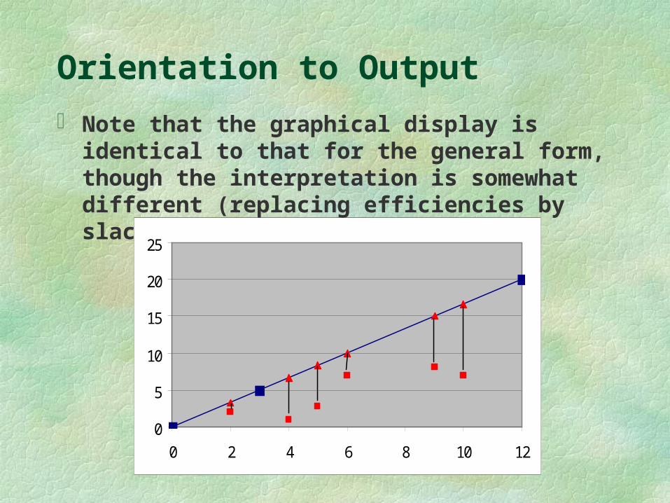
Orientation to Output
Note that the graphical display is identical to that for the general form, though the interpretation is somewhat different (replacing efficiencies by slacks).
0
5
10
15
20
25
0 2 4 6 8 10 12
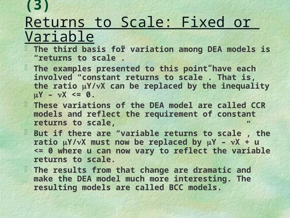
(3) Returns to Scale: Fixed or Variable
The third basis for variation among DEA models is “returns to scale”.
The examples presented to this point have each involved “constant returns to scale”. That is, the ratio Y/X can be replaced by the inequality Y – X <= 0.
These variations of the DEA model are called CCR models and reflect the requirement of constant returns to scale,
But if there are “variable returns to scale”, the ratio Y/X must now be replaced by Y – X + u <= 0 where u can now vary to reflect the variable returns to scale.
The results from that change are dramatic and make the DEA model much more interesting. The resulting models are called BCC models.
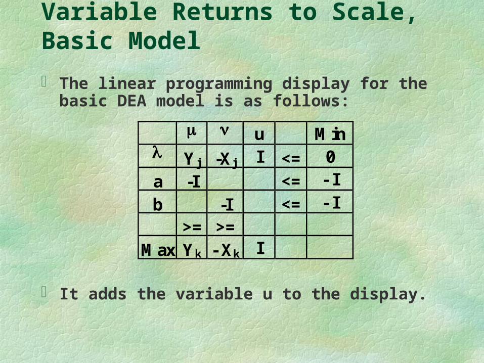
Variable Returns to Scale, Basic Model
The linear programming display for the basic DEA model is as follows:
It adds the variable u to the display.
u Min Yj -Xj I <= 0
a -I <= - I
b -I <= - I
>= >=
Max Yk - Xk I
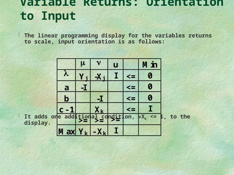
Variable Returns: Orientation to Input
The linear programming display for the variables returns to scale, input orientation is as follows:
It adds one additional condition, Xk <= 1, to the display.
u Min Yj -Xj I <= 0
a -I <= 0
b -I <= 0
c - 1 Xk <= I
>= >= >=
Max Yk - Xk I
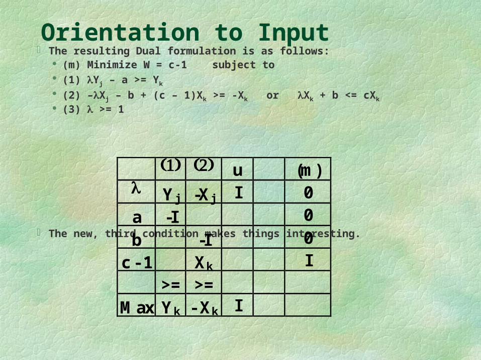
Orientation to Input The resulting Dual formulation is as follows:
(m) Minimize W = c-1 subject to (1) Yj – a >= Yk
(2) –Xj – b + (c – 1)Xk >= -Xk or Xk + b <= cXk
(3) >= 1
The new, third condition makes things interesting.
u (m) Yj -Xj I 0
a -I 0
b -I 0
c - 1 Xk I
>= >=
Max Yk - Xk I
Orientation to InputContinuing with the same example, the
following table shows the solutions in both formulations. The target is W = c – 1. Values to be varied are now (, a, b, c) or (u.
X Y W=c-1 a b u L1 2 2 0.00 0.00 =1.00 0.00 0.00 0.00 L2 3 5 0.00 0.00 1.00 0.00 0.00 0.00 L3 6 7 0.00 0.00 1.00 0.00 0.00 0.00 L4 9 8 0.00 0.00 1.00 0.00 0.00 0.00 L5 5 3 - 4.00 2.00 1.00 0.00 0.00 0.00 L6 4 1 - 5.00 4.00 1.00 0.00 0.00 0.00 L7 10 7 - 4.00 0.00 1.00 0.00 0.00 0.00

Orientation to Input
0
2
4
6
8
10
12
0 2 4 6 8 10 12

Orientation to Output
The linear programming display for the output orientation is as follows:
It adds one additional condition, Yk <= 1, to the display.
Min Yj -Xj <= 0
a -I <= 0
b -I <= 0
c - 1 Yk <= I
>= >=
Max Yk - Xk
Orientation to Output
The resulting Dual formulation is as follows: (m) Minimize W = 1 – c subject to (1) Yj – a >= cYk
(2) –Xj – b >= – Xk or Xk + b <= Xk
(m) Yj -Xj 0
a -I 0
b -I 0
1 - c Yk I
>= >=
Max Yk - Xk

Orientation to Output Continuing with the same example, the following table shows the
solutions in both formulations. The target is W = 1 – c. Values to be varied are still (, a, b, c) or ( and .
Note that L2 still dominates the solution, but the graph is now quite different,
X Y W=1-c a b L1 2 2 - 0.67 = 0.67 0.50 0.83 L2 3 5 0.00 0.20 0.33 L3 6 7 - 0.43 0.14 0.24 L4 9 8 - 0.87 0.13 0.21 L5 5 3 - 1.78 0.33 0.56 L6 4 1 - 5.67 1.00 1.67 L7 10 7 - 1.38 0.14 0.24
Orientation to Output
Note that the graphical display is identical to that for the general form, though the interpretation is somewhat different (replacing efficiencies by slacks).
0
5
10
15
20
25
0 2 4 6 8 10 12
Extensions to include a priori Valuations
To this point, DEA has been essentially a mathematical process in which the data for input and output are taken as given, without further interpretation with respect to the reality of operations.
But reality needs to be recognized, so there are several extensions that can be made to the basic DEA model, applicable to any of the variations.
They fall into seven categories: (1) Discretionary and Non-discretionary Variables (2) Categorical Variables (3)A priori restrictions on Weights (4) Relationships between Weights on Variables (5) A priori assessments of Efficient Units (6) Substitutability of Variables (7) Discrimination among Efficient Units
Discretionary & Non-discretionary
In identifying input and output variables, one wants to include all that are relevant to the operation. For example, the level of output is determined not only by what the unit itself does but by the size of the market to which the output is delivered.
The result, though, is that some relevant variables, such as the size of the market, are not under the control of management. Such variables, called non-discretionary, are in contrast to those that are under management control, called discretionary.
In assessing efficiency, all variables are considered, but in determining the criterion function to be maximized or minimized, only the discretionary variables are included.
Categorical Variables
In the DEA model as so far presented, the variables are treated as essentially quantitative, but sometimes one would like to identify non-quantitative variables, such as ordinal or nominal variables.
For example, one might like to compare institutions of the same type, such as public or private universities.
This is accomplished by introducing categorical variables containing numbers for order or identifiers for names.
A priori Restrictions on Weights
In the model as presented, the weights are limited only by the requirements that they be non-negative.
However, there may be reason to require that weights be further limited.
For example, it may be felt that a given variable must be included in the assessment so its weight must have at least a minimal value greater than zero. This might represent an output that is essential in assessment.
As another example, a variable may be such a large weight would over-emphasize its a priori importance so that there should be an upper limit on the weight. This might represent an output variable that is counter-productive.
Relationships between Weights
Sometimes, a priori knowledge may imply that there is a necessary relationship among variables. For example, an output variable may absolutely require some level of an input variable.
Such a priori knowledge may be expressed as a ratio between the weights assigned to the related variables.
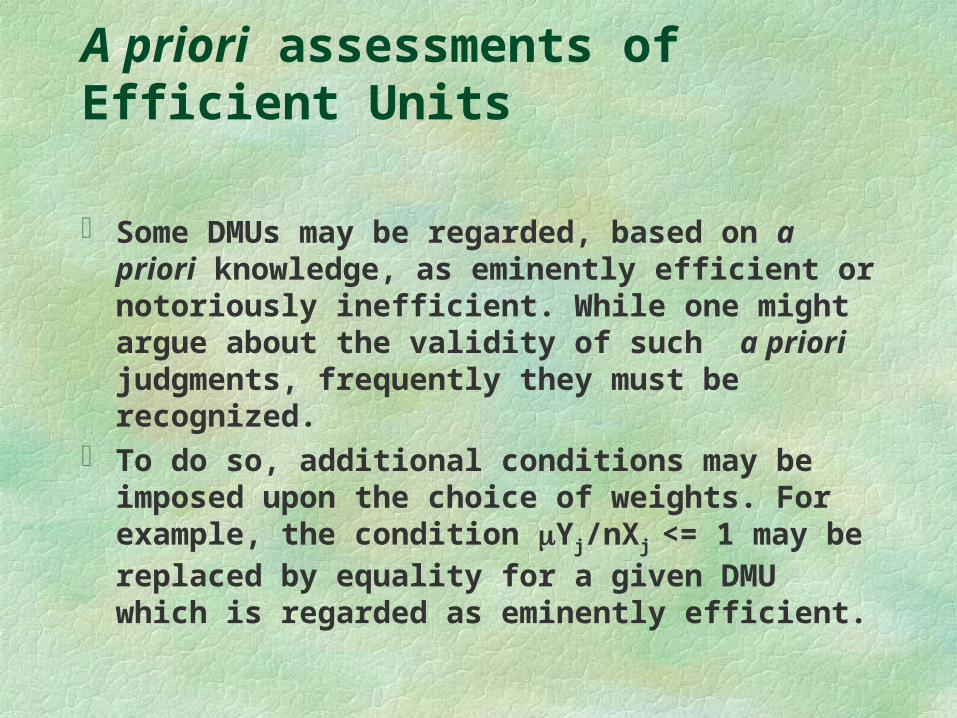
A priori assessments of Efficient Units
Some DMUs may be regarded, based on a priori knowledge, as eminently efficient or notoriously inefficient. While one might argue about the validity of such a priori judgments, frequently they must be recognized.
To do so, additional conditions may be imposed upon the choice of weights. For example, the condition Yj/nXj <= 1 may be replaced by equality for a given DMU which is regarded as eminently efficient.
Substitutability of Variables
A still unresolved issue is the means for representing substitutability of variables. For example, two input variables may represent two different type of labor which may be, to some extent, substitutable for each other.
How is such substitutability to be incorporated? Let’s explore this issue a bit further since, by doing so,
we can illuminate some additional perspectives on the basic DEA model.

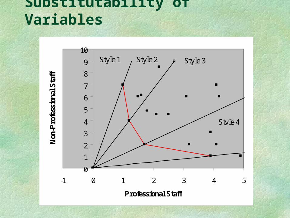
Substitutability of Variables
For simplicity in description, consider two input variables and a single output variable that has the same value for all DMUs. The graphic representation of the envelopment surface can now best be presented not in terms of the relationship between output and input, as previously shown, but between the variables of input.
The two variables are “Professional Staff” and “Non-Professional Staff”. The assumption is that they are completely substitutable and that physicians differ only in their “styles” of providing service, represented by the mix of the two means for doing so.
The “efficient” DMUs are located on the red envelopment surface, which shows the minimums in use of variables.
Substitutability of Variables
0
1
2
3
4
5
6
7
8
9
10
-1 0 1 2 3 4 5
Professional Staff
Non
-Pro
fess
iona
l Sta
ffStyle 1
Style 4
Style 2 Style 3

Discrimination among Efficient Units
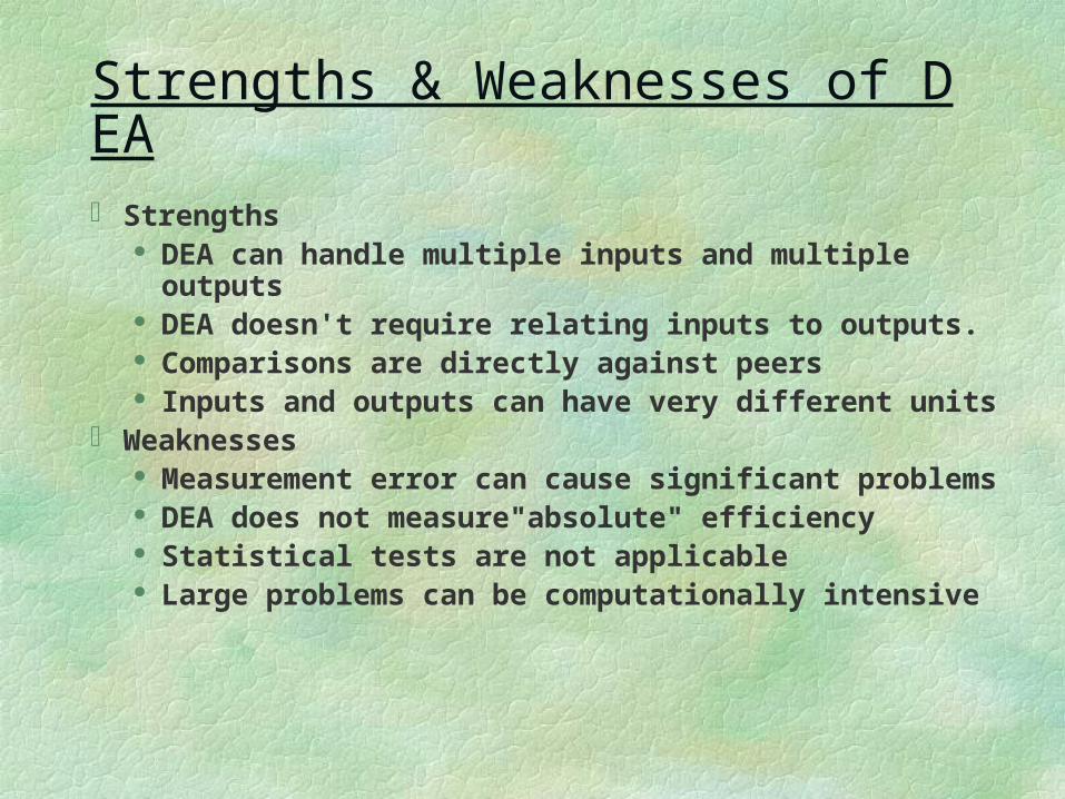
Strengths & Weaknesses of DEA
Strengths DEA can handle multiple inputs and multiple outputs DEA doesn't require relating inputs to outputs. Comparisons are directly against peers Inputs and outputs can have very different units
Weaknesses Measurement error can cause significant problems DEA does not measure"absolute" efficiency Statistical tests are not applicable Large problems can be computationally intensive
Implementation of DEA
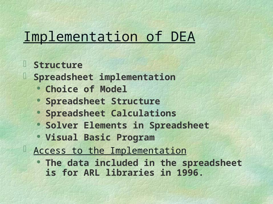
Structure Spreadsheet implementation
Choice of Model Spreadsheet Structure Spreadsheet Calculations Solver Elements in Spreadsheet Visual Basic Program
Access to the Implementation The data included in the spreadsheet is for ARL
libraries in 1996.
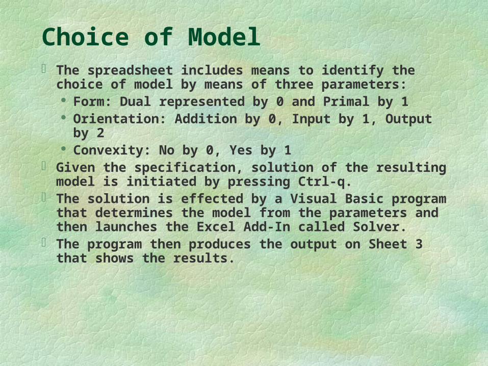
Choice of Model The spreadsheet includes means to identify the choice of
model by means of three parameters: Form: Dual represented by 0 and Primal by 1 Orientation: Addition by 0, Input by 1, Output by 2 Convexity: No by 0, Yes by 1
Given the specification, solution of the resulting model is initiated by pressing Ctrl-q.
The solution is effected by a Visual Basic program that determines the model from the parameters and then launches the Excel Add-In called Solver.
The program then produces the output on Sheet 3 that shows the results.
Spreadsheet Structure
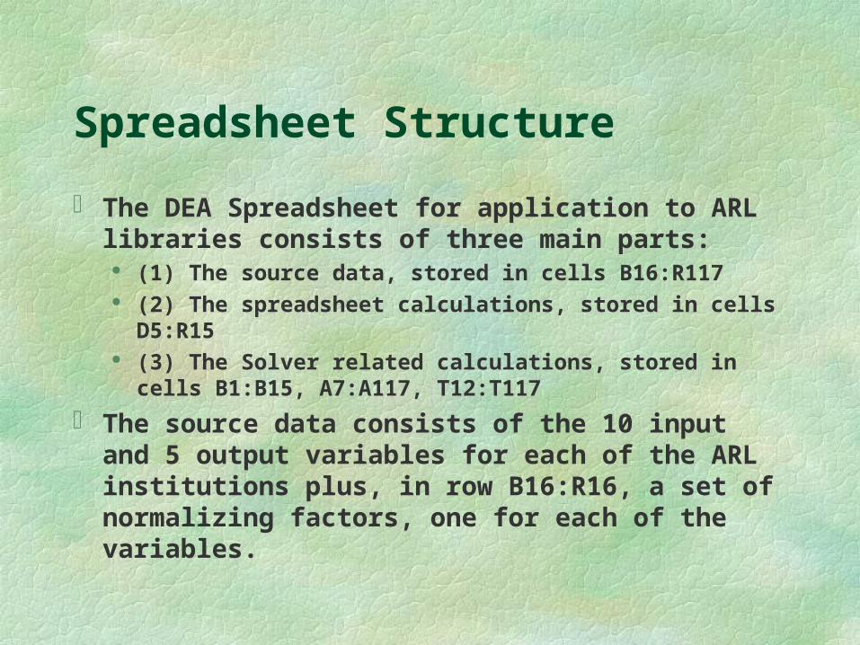
The DEA Spreadsheet for application to ARL libraries consists of three main parts:
(1) The source data, stored in cells B16:R117 (2) The spreadsheet calculations, stored in cells D5:R15 (3) The Solver related calculations, stored in cells
B1:B15, A7:A117, T12:T117
The source data consists of the 10 input and 5 output variables for each of the ARL institutions plus, in row B16:R16, a set of normalizing factors, one for each of the variables.
Spreadsheet Calculations
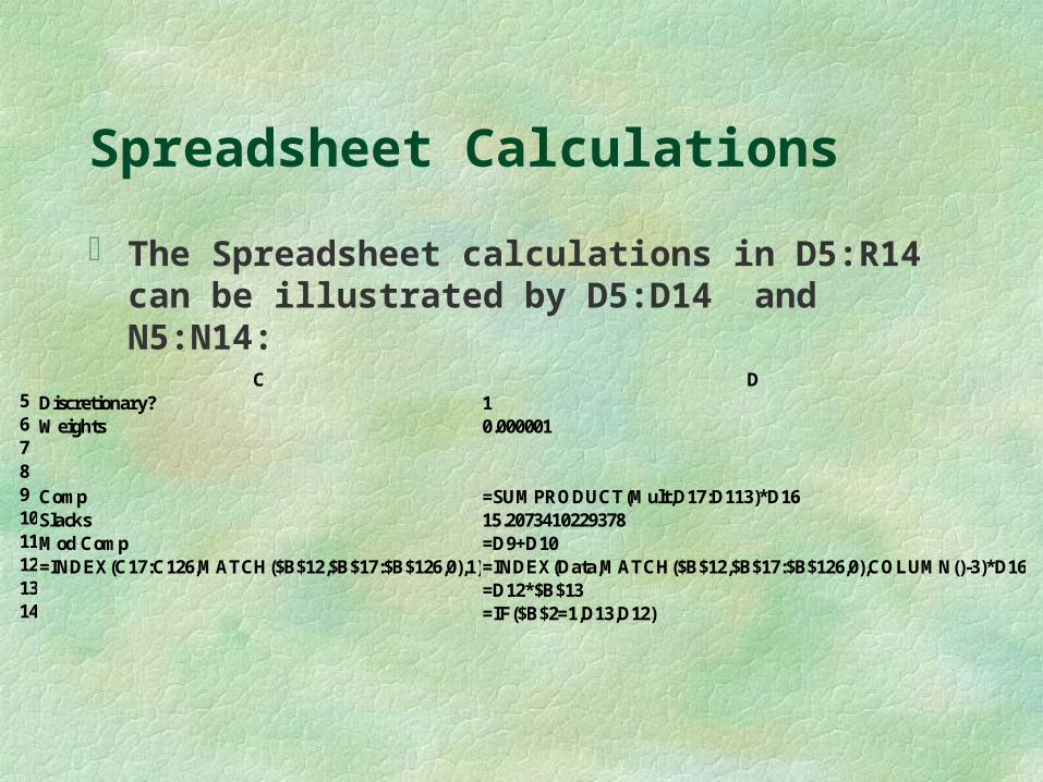
The Spreadsheet calculations in D5:R14 can be illustrated by D5:D14 and N5:N14:
C D 5 Discretionary? 1 6 Weights 0.000001 7 8 9 Comp =SUMPRODUCT(Mult,D17:D113)*D16 10 Slacks 15.2073410229378 11 Mod Comp =D9+D10 12 =INDEX(C17:C126,MATCH($B$12,$B$17:$B$126,0),1) =INDEX(Data,MATCH($B$12,$B$17:$B$126,0),COLUMN()-3)*D16 13 =D12*$B$13 14 =IF($B$2=1,D13,D12)
Spreadsheet Calculations
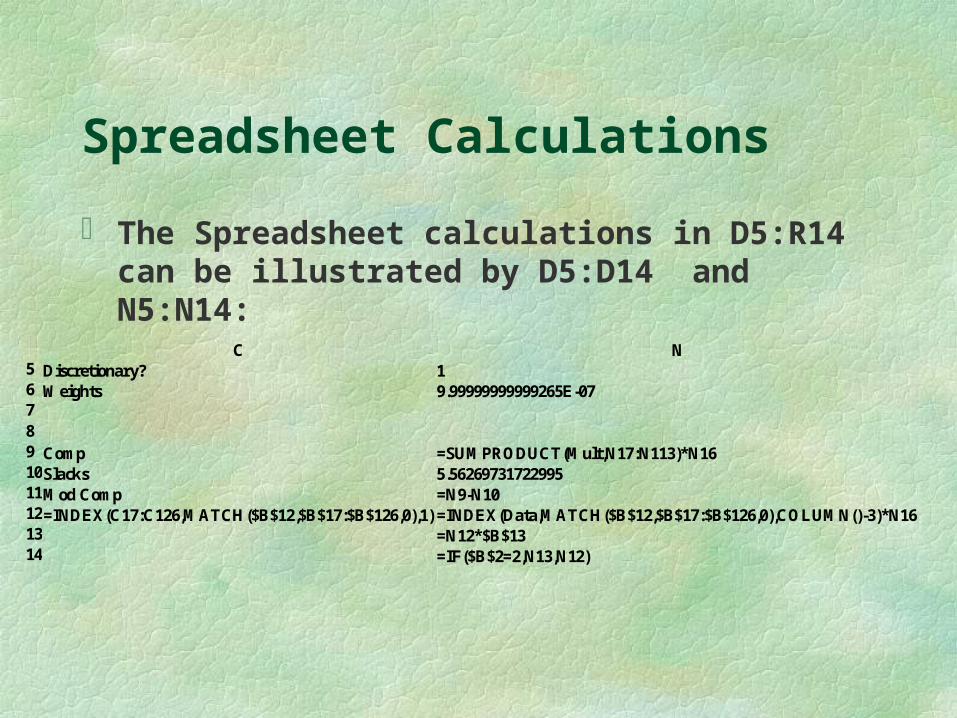
The Spreadsheet calculations in D5:R14 can be illustrated by D5:D14 and N5:N14:
C N 5 Discretionary? 1 6 Weights 9.99999999999265E-07 7 8 9 Comp =SUMPRODUCT(Mult,N17:N113)*N16 10 Slacks 5.56269731722995 11 Mod Comp =N9-N10 12 =INDEX(C17:C126,MATCH($B$12,$B$17:$B$126,0),1) =INDEX(Data,MATCH($B$12,$B$17:$B$126,0),COLUMN()-3)*N16 13 =N12*$B$13 14 =IF($B$2=2,N13,N12)
Solver Elements in Spreadsheet
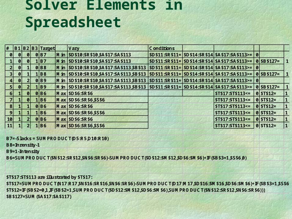
# B1 B2 B3 Target Vary Conditions0 0 0 0 B7 Min $D$10:$R$10,$A$17:$A$113 $D$11:$R$11= $D$14:$R$14 $A$17:$A$113>= 01 0 0 1 B7 Min $D$10:$R$10,$A$17:$A$113 $D$11:$R$11= $D$14:$R$14 $A$17:$A$113>= 0 $B$127= 12 0 1 0 B8 Min $D$10:$R$10,$A$17:$A$113,$B$13 $D$11:$R$11= $D$14:$R$14 $A$17:$A$113>= 03 0 1 1 B8 Min $D$10:$R$10,$A$17:$A$113,$B$13 $D$11:$R$11= $D$14:$R$14 $A$17:$A$113>= 0 $B$127= 14 0 2 0 B9 Min $D$10:$R$10,$A$17:$A$113,$B$13 $D$11:$R$11= $D$14:$R$14 $A$17:$A$113>= 05 0 2 1 B9 Min $D$10:$R$10,$A$17:$A$113,$B$13 $D$11:$R$11= $D$14:$R$14 $A$17:$A$113>= 0 $B$127= 16 1 0 0 B6 Max $D$6:$R$6 $T$17:$T$113<= 0 $T$12= 17 1 0 1 B6 Max $D$6:$R$6,$S$6 $T$17:$T$113<= 0 $T$12= 18 1 1 0 B6 Max $D$6:$R$6 $T$17:$T$113<= 0 $T$12= 19 1 1 1 B6 Max $D$6:$R$6,$S$6 $T$17:$T$113<= 0 $T$12= 1
10 1 2 0 B6 Max $D$6:$R$6 $T$17:$T$113<= 0 $T$12= 111 1 2 1 B6 Max $D$6:$R$6,$S$6 $T$17:$T$113<= 0 $T$12= 1
B7=-Slacks = SUMPRO DUCT(D5:R5,D10:R10)B8=Inrensity-1B9=1-IntensityB6=SUMPRO DUCT($N$12:$R$12,$N$6:$R$6)-SUMPRO DUCT($D$12:$M$12,$D$6:$M$6)+IF($B$3=1,$S$6,0)
$T$17:$T$113 are il lustrated by $T$17:$T$17=SUMPRO DUCT(N17:R17,$N$16:$R$16,$N$6:$R$6)-SUMPRO DUCT(D17:M17,$D$16:$M$16,$D$6:$M$6)+IF($B$3=1,$S$6,0)$T$12=IF($B$2=0,1,IF($B$2=1,SUMPRO DUCT($D$12:$M$12,$D$6:$M$6),SUMPRO DUCT($N$12:$R$12,$N$6:$R$6)))$B$127=SUM($A$17:$A$117)
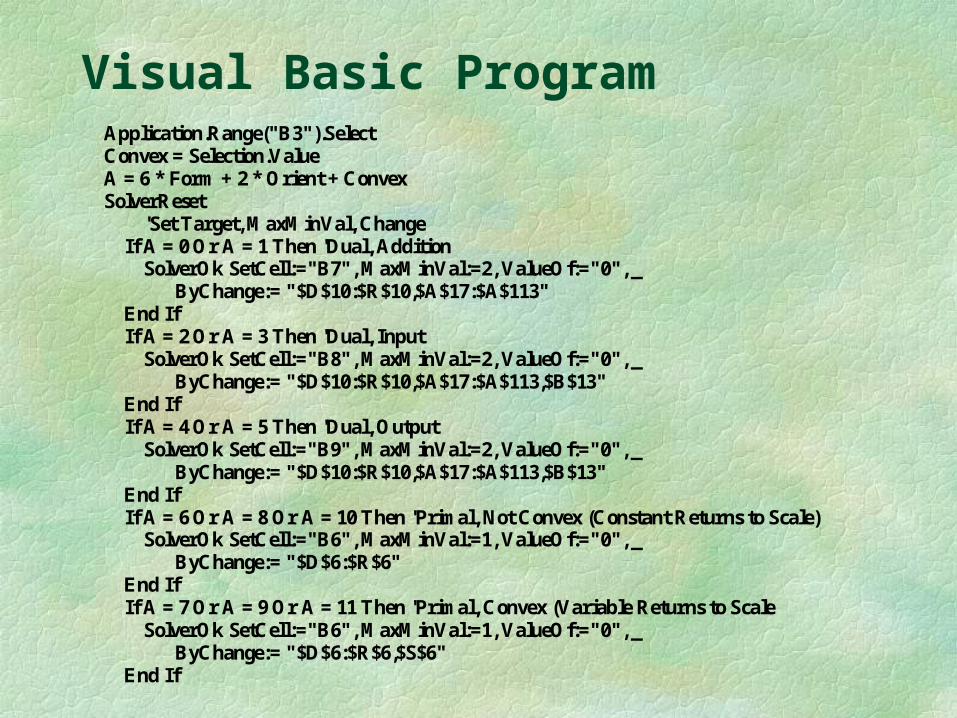
Visual Basic ProgramApplication.Range("B3").Select Convex = Selection.Value A = 6 * Form + 2 * Orient + Convex SolverReset 'Set Target, MaxMinVal, Change If A = 0 Or A = 1 Then 'Dual, Addition SolverOk SetCell:="B7", MaxMinVal:=2, ValueOf:="0", _
ByChange:= "$D$10:$R$10,$A$17:$A$113" End If If A = 2 Or A = 3 Then 'Dual, Input SolverOk SetCell:="B8", MaxMinVal:=2, ValueOf:="0", _
ByChange:= "$D$10:$R$10,$A$17:$A$113,$B$13" End If If A = 4 Or A = 5 Then 'Dual, Output SolverOk SetCell:="B9", MaxMinVal:=2, ValueOf:="0", _
ByChange:= "$D$10:$R$10,$A$17:$A$113,$B$13" End If If A = 6 Or A = 8 Or A = 10 Then 'Primal, Not Convex (Constant Returns to Scale) SolverOk SetCell:="B6", MaxMinVal:=1, ValueOf:="0", _
ByChange:= "$D$6:$R$6" End If If A = 7 Or A = 9 Or A = 11 Then 'Primal, Convex (Variable Returns to Scale SolverOk SetCell:="B6", MaxMinVal:=1, ValueOf:="0", _
ByChange:= "$D$6:$R$6,$S$6" End If
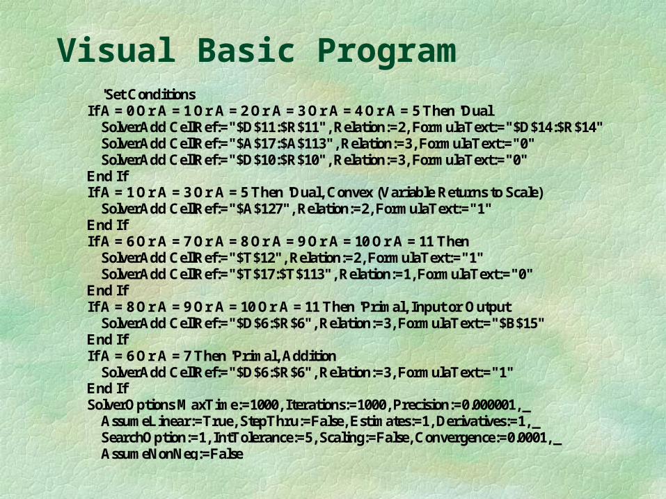
Visual Basic Program 'Set Conditions If A = 0 Or A = 1 Or A = 2 Or A = 3 Or A = 4 Or A = 5 Then 'Dual SolverAdd CellRef:="$D$11:$R$11", Relation:=2, FormulaText:="$D$14:$R$14" SolverAdd CellRef:="$A$17:$A$113", Relation:=3, FormulaText:="0" SolverAdd CellRef:="$D$10:$R$10", Relation:=3, FormulaText:="0" End If If A = 1 Or A = 3 Or A = 5 Then 'Dual, Convex (Variable Returns to Scale) SolverAdd CellRef:="$A$127", Relation:=2, FormulaText:="1" End If If A = 6 Or A = 7 Or A = 8 Or A = 9 Or A = 10 Or A = 11 Then SolverAdd CellRef:="$T$12", Relation:=2, FormulaText:="1" SolverAdd CellRef:="$T$17:$T$113", Relation:=1, FormulaText:="0" End If If A = 8 Or A = 9 Or A = 10 Or A = 11 Then 'Primal, Input or Output SolverAdd CellRef:="$D$6:$R$6", Relation:=3, FormulaText:="$B$15" End If If A = 6 Or A = 7 Then 'Primal, Addition SolverAdd CellRef:="$D$6:$R$6", Relation:=3, FormulaText:="1" End If SolverOptions MaxTime:=1000, Iterations:=1000, Precision:=0.000001, _ AssumeLinear:=True, StepThru:=False, Estimates:=1, Derivatives:=1, _ SearchOption:=1, IntTolerance:=5, Scaling:=False, Convergence:=0.0001, _ AssumeNonNeg:=False
Visual Basic Program
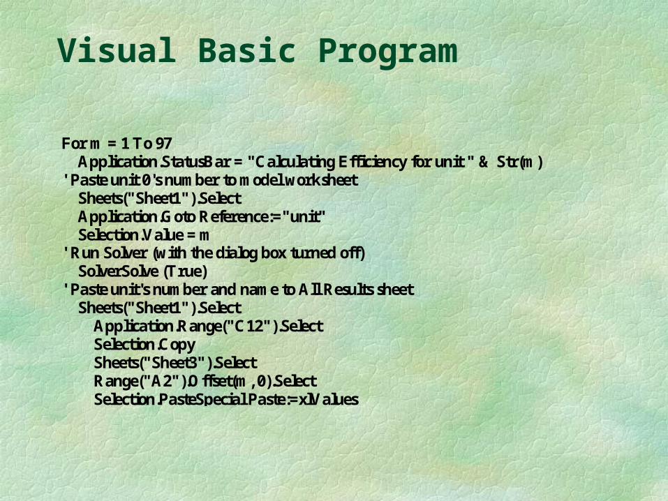
For m = 1 To 97 Application.StatusBar = "Calculating Efficiency for unit " & Str(m) ' Paste unit 0's number to model worksheet Sheets("Sheet1").Select Application.Goto Reference:="unit" Selection.Value = m ' Run Solver (with the dialog box turned off) SolverSolve (True) ' Paste unit's number and name to All Results sheet Sheets("Sheet1").Select Application.Range("C12").Select Selection.Copy Sheets("Sheet3").Select Range("A2").Offset(m, 0).Select Selection.PasteSpecial Paste:=xlValues
Visual Basic Program
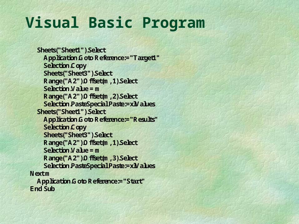
Sheets("Sheet1").Select Application.Goto Reference:="Target1" Selection.Copy Sheets("Sheet3").Select Range("A2").Offset(m, 1).Select Selection.Value = m Range("A2").Offset(m, 2).Select Selection.PasteSpecial Paste:=xlValues Sheets("Sheet1").Select Application.Goto Reference:="Results" Selection.Copy Sheets("Sheet3").Select Range("A2").Offset(m, 1).Select Selection.Value = m Range("A2").Offset(m, 3).Select Selection.PasteSpecial Paste:=xlValues Next m Application.Goto Reference:="Start" End Sub
The Example of Libraries
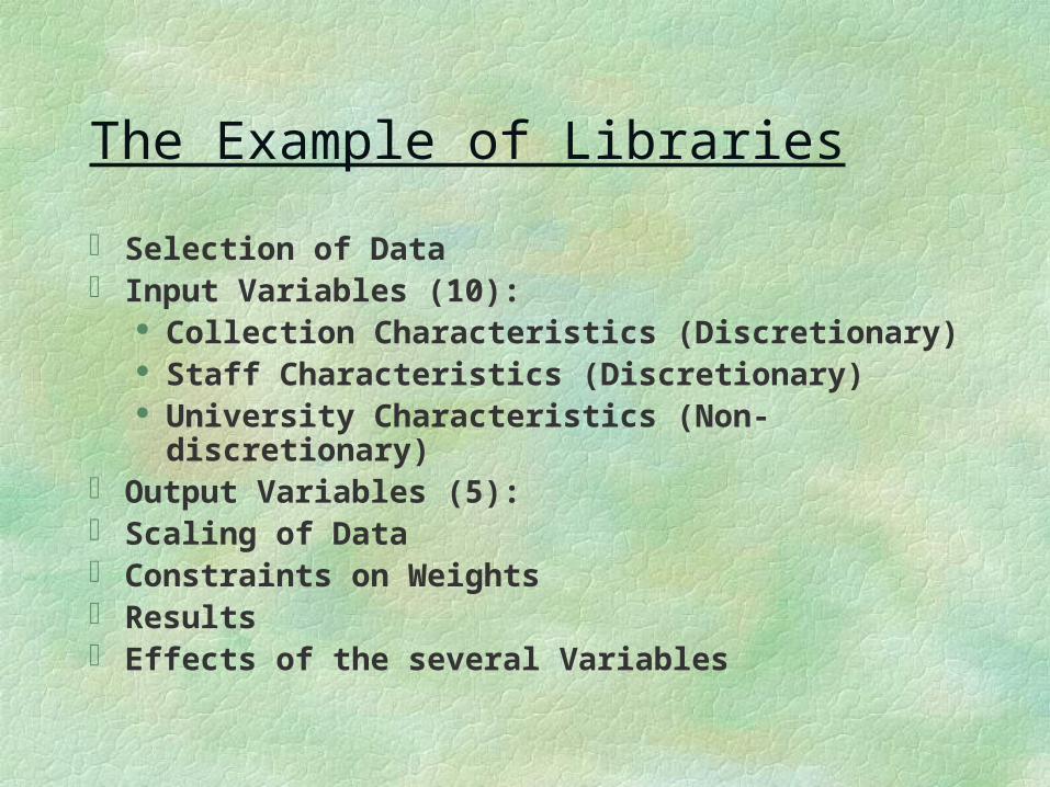
Selection of Data Input Variables (10):
Collection Characteristics (Discretionary) Staff Characteristics (Discretionary) University Characteristics (Non-discretionary)
Output Variables (5): Scaling of Data Constraints on Weights Results Effects of the several Variables

Selection of Data

The Variables

Scaling of the Variables

Constraints on Weights

Results
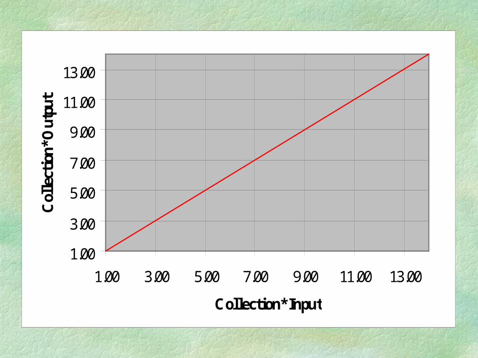
Efficiency Distribution
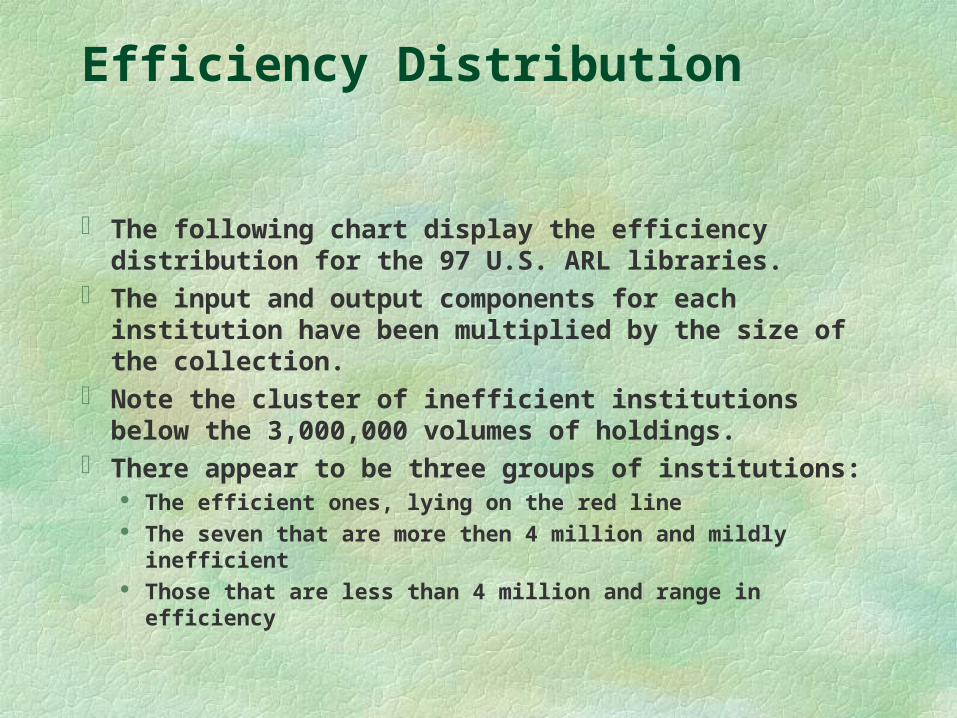
The following chart display the efficiency distribution for the 97 U.S. ARL libraries.
The input and output components for each institution have been multiplied by the size of the collection.
Note the cluster of inefficient institutions below the 3,000,000 volumes of holdings.
There appear to be three groups of institutions: The efficient ones, lying on the red line The seven that are more then 4 million and mildly inefficient Those that are less than 4 million and range in efficiency
1.00
3.00
5.00
7.00
9.00
11.00
13.00
1.00 3.00 5.00 7.00 9.00 11.00 13.00
Collection*Input
Col
lect
ion*
Out
put
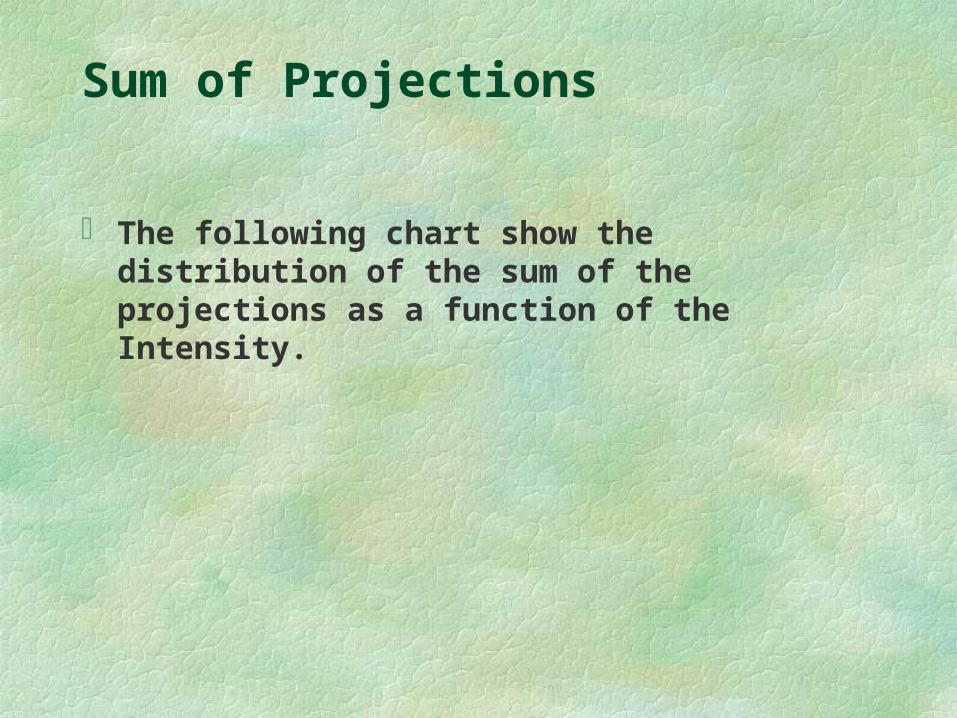
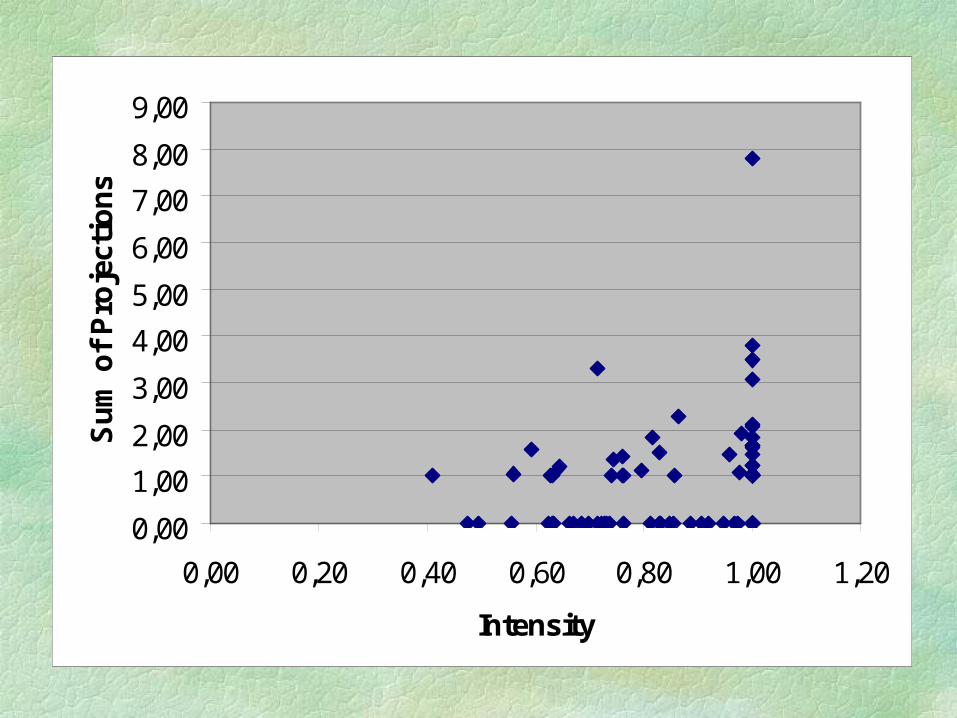
Sum of Projections
The following chart show the distribution of the sum of the projections as a function of the Intensity.
0,00
1,00
2,00
3,00
4,00
5,00
6,00
7,00
8,00
9,00
0,00 0,20 0,40 0,60 0,80 1,00 1,20
Intensity
Su
m o
f P
roje
ctio
ns
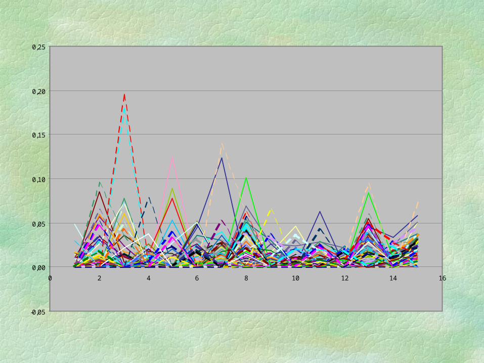
Distribution of Weights
The following chart shows the magnitudes of the weights on each of the Input and Output components
-0,05
0,00
0,05
0,10
0,15
0,20
0,25
0 2 4 6 8 10 12 14 16

Annals of Operations Research 66 (1996)
Preface
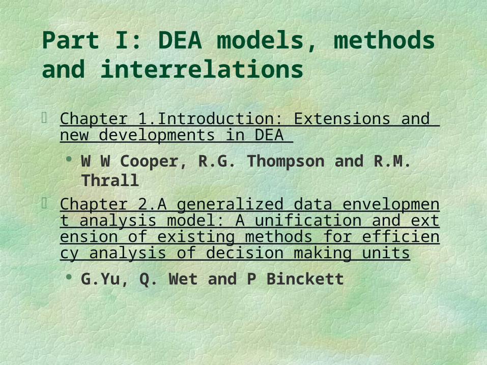
Part I: DEA models, methods and interrelations
Chapter 1.Introduction: Extensions and new developments in DEA
W W Cooper, R.G. Thompson and R.M. Thrall Chapter 2.A generalized data envelopment analysis model:
A unification and extension of existing methods for efficiency analysis of decision making units
G.Yu, Q. Wet and P Binckett
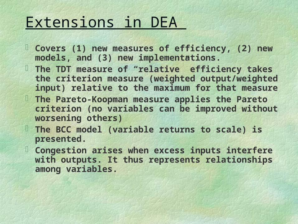
Extensions in DEA
Covers (1) new measures of efficiency, (2) new models, and (3) new implementations.
The TDT measure of “relative” efficiency takes the criterion measure (weighted output/weighted input) relative to the maximum for that measure
The Pareto-Koopman measure applies the Pareto criterion (no variables can be improved without worsening others)
The BCC model (variable returns to scale) is presented. Congestion arises when excess inputs interfere with
outputs. It thus represents relationships among variables.
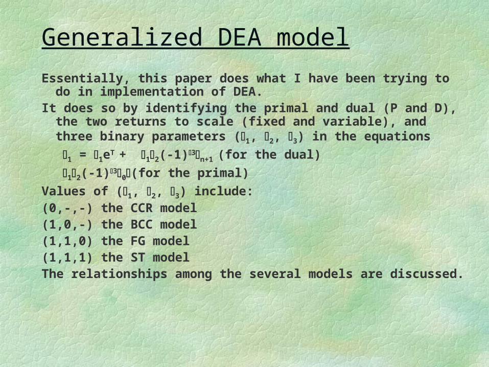
Generalized DEA modelEssentially, this paper does what I have been trying to do in implementation
of DEA.It does so by identifying the primal and dual (P and D), the two returns to
scale (fixed and variable), and three binary parameters (1, 2, 3) in the equations
1 = 1eT + 12(-1)3n+1 (for the dual)
12(-1)30(for the primal)
Values of (1, 2, 3) include:(0,-,-) the CCR model(1,0,-) the BCC model(1,1,0) the FG model(1,1,1) the ST modelThe relationships among the several models are discussed.

Part II: Desirable properties of models, measures and solutions (1)
Chapter 3. Translation invariance in data envelopment analysis: A generalization
J.T Pastor Chapter 4. The lack of invariance of optimal dual solutions
under translation R.M. Thrall
Chapter 5. Duality, classification and slacks in DEA R.M. Thrall
Translation invariance
This paper proves that several of the DEA model are translation invariant (i.e., optimal solutions are not changed if the original variable values are “translated”, that is all values for a variable are replaced by some constant minus the values).
Specifically, the primal additive model is translation invariant.
The BCC input oriented primal model is output translation invariant.
The CCR models are not translation invariant.
Lack of invariance
This paper supplements the prior one. It shows that in neither the BCC model nor the additive model are the optimal solutions for the dual (i.e., multipler) formulation invariant under translation.
Duality, classification and slack This paper considers the role of slacks especially in the context of
radial measures of efficiency. The effect of alternative optima is to make slacks difficult to deal with; the theory presented resolves the difficulties.
The CCT model presented eliminates the need for non-Archimedean models and permits dealing with zero values for the variables.
The concept of an “admissible virtual multiplier” is introduced and the maximizing virtual multiplier w* is the basis for categorizing efficient DMUs into 3 groups:
Extreme Efficient: all variables are included in w* Efficient: the variables in w* are all positive Weak efficient: w* has at least one zero variable
Similarly for non-efficient DMUs
Part II: Desirable properties of models, measures and solutions (2)
Chapter 6. On the construction of strong complementarity slackness solutions for DEA linear programming problems using a primal-dual interior-point method
M.D. Gonzdlez-Ltma, R.A. Tapta and R.M. Thralt Chapter 7. DEA multiplier analytic center sensitivity with
an illustrative application to independent oil companies R.C. Thompson, PS. Ditarmapala, f Diaz, M.D.
Gonzdlez-Lima and R.M. Thrall
Complementarity Slackness Solutions This paper proposes use of “primary-dual interior-point
methods” for solution of the DEA linear programming problem (an iterative process that generates interior point that converge to the solution).
The primary form minimizes C’x; the dual form maximizes B’y.
The condition for solution is that C’x = B’y, called the complementarity slackness condition.
These methods attempt to solve the primary and dual linear programs simultaneously.
Solutions are classified as radially efficient or inefficient using the CCT model.
Multiplier Sensitivity
The stability of the set E of extreme efficient DMUs is examined to determine the sensitivity to changes in the data,

Part III: Frontier shifts and efficiency evaluations
Chapter 8. Estimating production frontier shifts: An application of DEA to technology assessment
R.D. Banker and R.C. Morey Chapter 9. Moving frontier analysis: An application of
data envelopment analysis for competitive analysis of a high-technology manufacturing plant
K.K. Sinha Chapter 10. Profitability and productivity changes: An
application to Swedish pharmacies R. Aithin, R. Fare and S. Grosskopf 219

Production Frontier Shifts
This paper divides the set of DMUs into two categories (representing the use or non-use of a technology). For a DMU without the technology, comparison is made only with others without the technology; for those with the technology, comparison is made with all DMUs.
The result is a basis for assessment of the impact of the technology.
Moving Frontier Analysis
This paper proposes a method for assessing when some data may not be available. It uses aggregate data on “best practices”. It depends upon time series data

Profitability & productivity changes
It is not evident how this relates to DEA.
Part IV: Statistical and stochastic characterizations
Chapter 11. Simulation studies of efficiency, returns to scale and misspecification with nonlinear functions in DEA
RD. Banker; H. Chang and WW Cooper Chapter 12. New uses of DEA and statistical regressions for
efficiency evaluation and estimation - with an illustrative application to public secondary schools in Texas
VL Arnold, LR. Bardhan, WW Cooper and S.C. Kumbhakar
Chapter 13. Satisficing DEA models under chance constraints
W W Cooper Z Huang and S.X. Li

Simulation studies
Well, so be it.
DEA and statistical regressions
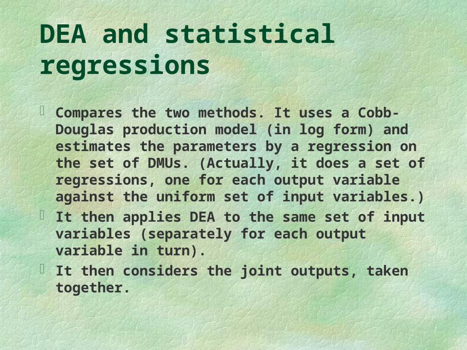
Compares the two methods. It uses a Cobb-Douglas production model (in log form) and estimates the parameters by a regression on the set of DMUs. (Actually, it does a set of regressions, one for each output variable against the uniform set of input variables.)
It then applies DEA to the same set of input variables (separately for each output variable in turn).
It then considers the joint outputs, taken together.
Satisficing DEA models
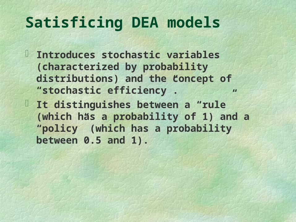
Introduces stochastic variables (characterized by probability distributions) and the concept of “stochastic efficiency”.
It distinguishes between a “rule” (which has a probability of 1) and a “policy” (which has a probability between 0.5 and 1).
Part V: Some new applications
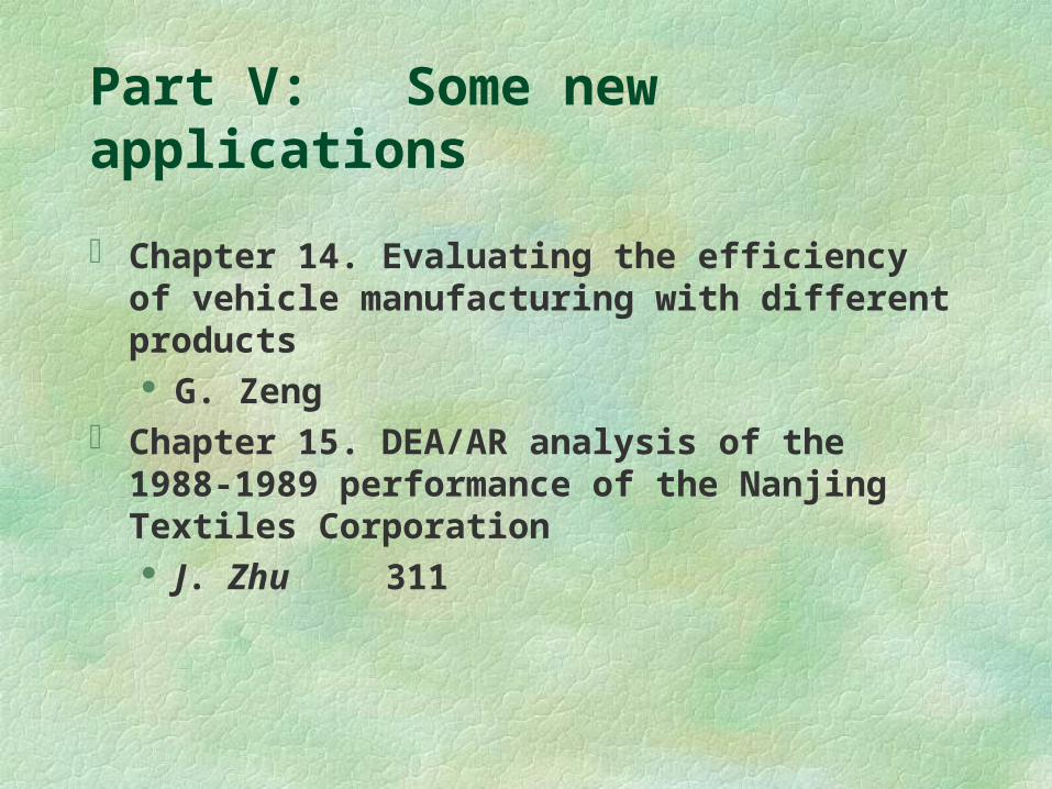
Chapter 14. Evaluating the efficiency of vehicle manufacturing with different products
G. Zeng Chapter 15. DEA/AR analysis of the 1988-1989
performance of the Nanjing Textiles Corporation J. Zhu 311

China vehicle manufacturing
Evaluates the efficiency of vehicle manufacturing in China.
It deals with the problem of zero values for some variables.

DEA/AR analysis
Another application in China.
Annals of Operations Research 73 (1997)ContentsPrefaceForeword

Part VI: Extending Frontiers
Extending the frontiers of Data Envelopment Analysis A.Y Lewin and LM. Seijord
Weights restrictions and value judgements in Data Envelopment Analysis: Evolution, development and future directions
R.Allen, A. Athanassopoulos, R.O. Dyson and F. Thanassoulis

Extending the frontiers
See earlier in this presentation

Weights restrictions & value judgments
See earlier in this presentation.

Part VII: Applications
DEA and primary care physician report cards: Deriving preferred practice cones from managed care service concepts and operating strategies
IA. Chilingerian and H.D. Sherman An analysis of staffing efficiency in U.S.
manufacturing: 1983 and 1989 PT Ward, J.E. Storbeck, S.L. Mangum and RE
Byrnes Applications of DEA to measure the efficiency of
software production at two large Canadian banks J.C. Paradi, D.N. Reese and D. Rosen

Primary care physician
This papers identifies “styles” of management based on ratios of input variables aimed at input cost minimizing.
The example used is comparison of hospital days versus office visits
Staffing efficiency
Again, styles of management are identified, this time based on ratios of types of staffing (e.g., professional vs. non-professional). Industries are divided into types (batch vs. line processing industries) and “best practices” for each type are identified by DEA.
software production
Input to software production is taken as cost; outputs as size (measure by “function points”), quality (measured by defects or rework hours), and time to market.
The DEA is compared to performance ratio analyses, such as Cost/Function, Defects/Function, Days/Function.
Then, constraints on the weights are introduced. One set of constraints consisted of bounds on ratios of weights. A second set of constraints consisted of tradeoffs between variables, again represented by bounds on ratios.

Part VII: Applications
Restricted best practice selection in DEA: An overview with a case study evaluating the socio-economic performance of nations
B.Golany and S. Thore A new measure of baseball batters using DEA
T.R. Anderson and G.P Sharp Efficiency of families managing home health care
CE. Smith, S. VM. Kiembeck, K. Fernengel and L.S. Mayer

Economic performance of nations
To apply DEA to evaluation of economic performance of nations, it is necessary to recognize some constraints:
International requirements (treaties, bilateral agreements) Externalities (e.g., mandated quotas) Issues of equity
These constraints are then incorporated into DEA
Baseball batters
Traditional methods for evaluating batters include fixed and variable weight statistics (homers, batting average, slugging average, RBI, etc.). The point in this article is that use of DEA allows one to determine the effect of changes over time.
Another effect of interest is “noise”. To correct for noise, the DEA model “derates” the data for each player by a factor based on the player’s standard deviation for each variable
Efficiency of families
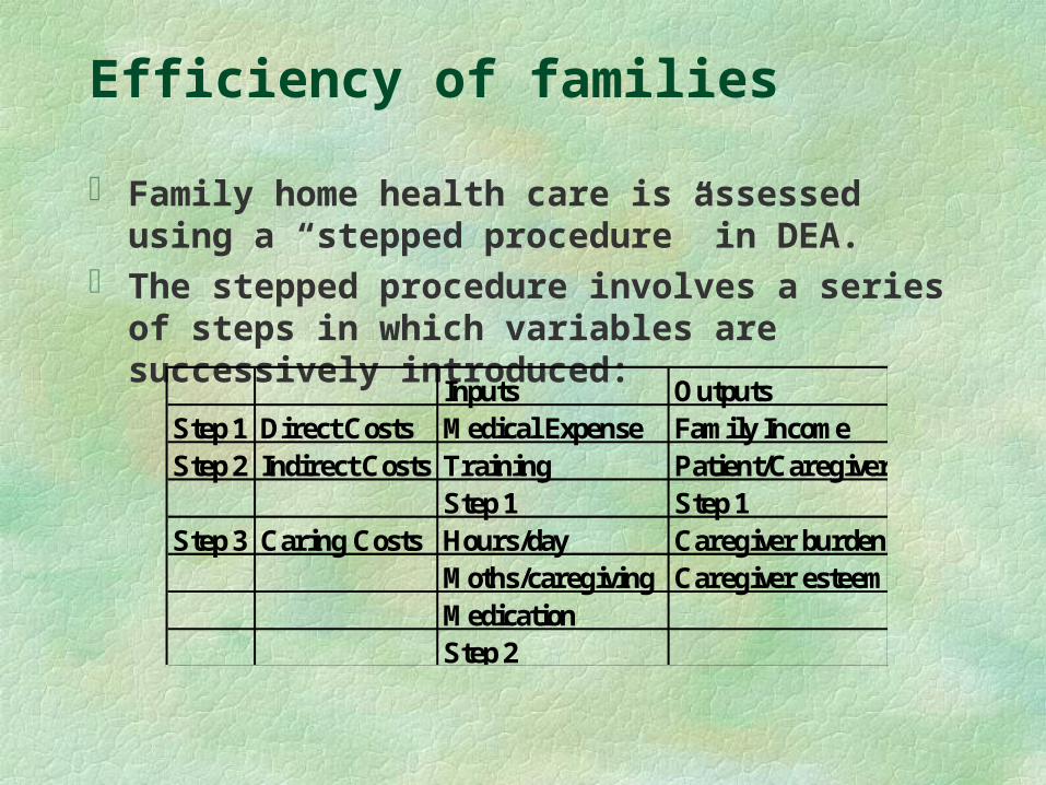
Family home health care is assessed using a “stepped procedure” in DEA.
The stepped procedure involves a series of steps in which variables are successively introduced:
Inputs OutputsStep 1 Direct Costs Medical Expense Family IncomeStep 2 Indirect Costs Training Patient/Caregiver
Step 1 Step 1Step 3 Caring Costs Hours/day Caregiver burden
Moths/caregiving Caregiver esteemMedicationStep 2

Part VII: Applications
A DEA-based analysis of productivity change and intertemporal managerial performance
E.Grifell-Tatje and C.A.K. LoveII Use of Data Envelopment Analysis in assessing
Information Technology impact on firm performance C.H. Wang, R.D. Gopal and S. Zionts

Productivity & managerial performance
Examines the productivity of an organization over time.

Information Technology impact
Examines the impact of information technology on performance of firms. It divides operations into two stages: (1) Accumulation of resources and (2) Use of resources. (These are illustrated in banking by (1) the collection of funds from depositors and (2) use of those funds for generating income).
It examines separately the effect of information technology (represented by ATM machines) on the two stages.
Part VIII: Theoretical Extensions
Comparative advantage and disadvantage in DEA A.I. Alt and CS. LeTine
Model misspecification in Data Envelopment Analysis P Smith
Dominant Competitive Factors for evaluating program efficiency in grouped data
J.J.Rousseau and J.H. Semple DEA-based yardstick competition. The optimality of
best practice regulation P Bogetoft
Comparative advantage & disadvantage
This paper introduces a cost function into DEA analysis as the means for calculating a comparative advantage or disadvantage as the difference between the costs of input and the income from output.
It interprets the weights in each DMUs optimum as prices for the respective inputs and outputs. The result is “virtual” cost, revenue, and profit. The profit (or loss) is then compared with the maximum profit obtained by a best practice unit and that of the evaluated unit.
For an efficient unit, the comparison is between the virtual profit of the valuated unit and the maximum profit across all other units.
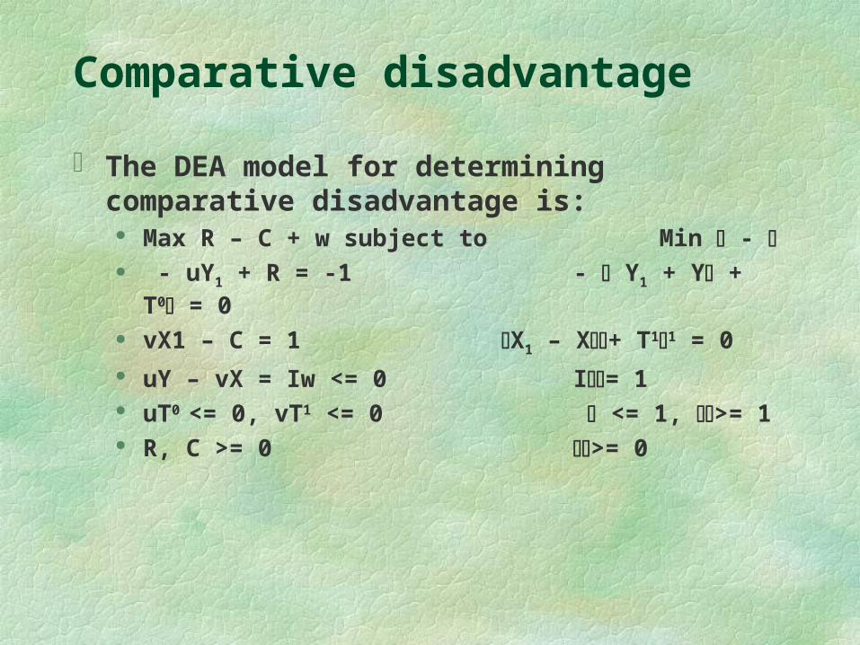
Comparative disadvantage
The DEA model for determining comparative disadvantage is:
Max R – C + w subject to Min - - uY1 + R = -1 - Y1 + Y + T0 = 0
vX1 – C = 1 X1 – X+ T11 = 0 uY – vX = Iw <= 0 I= 1 uT0 <= 0, vT1 <= 0 <= 1, >= 1 R, C >= 0 >= 0
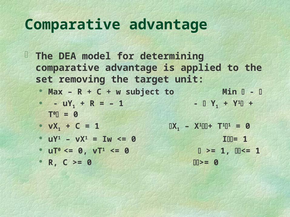
Comparative advantage
The DEA model for determining comparative advantage is applied to the set removing the target unit:
Max – R + C + w subject to Min - - uY1 + R = – 1 - Y1 + Y1 + T0 = 0
vX1 + C = 1 X1 – X1+ T11 = 0 uY1 – vX1 = Iw <= 0 I= 1 uT0 <= 0, vT1 <= 0 >= 1, <= 1 R, C >= 0 >= 0
Model mis-specification
This paper examines the effects of various types of mis-specifications of the DEA model. They include:
Omission of a necessary input Inclusion of an extraneous variable Erroneous assumption about returns to scale
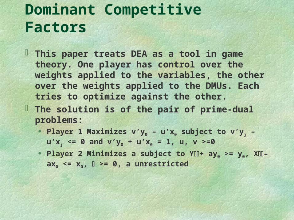
Dominant Competitive Factors
This paper treats DEA as a tool in game theory. One player has control over the weights applied to the variables, the other over the weights applied to the DMUs. Each tries to optimize against the other.
The solution is of the pair of prime-dual problems: Player 1 Maximizes v’y0 – u’x0 subject to v’yj – u’xj <= 0 and
v’y0 + u’x0 = 1, u, v >=0
Player 2 Minimizes a subject to Y+ ay0 >= y0, X– ax0 <= x0, >= 0, a unrestricted

Best practice regulation
The use of DEA in regulatory practice is discussed. The underlying game is represented by a series of steps:
Costs and demands for service are observed or identified Schemes are proposed by the regulator The schemes are rejected or accepted by the DMUs Costs are selected by the DMUs Data on performance are observed Compensations are paid
The aim of the regulator is to minimize the expected costs of making the DMUs accept, fulfil, and minimize costs.
The use of DEA is to determine the best practce norms.
Part VIII: Theoretical Extensions
A Data Envelopment Analysis approach to Discriminant Analysis
D.L. Retzlaff-Roberts Derivation of the Maximum Efficiency Ratio mode
from the maximum decisional efficiency principle M.D. Trouft
Discriminant Analysis
Discriminant analysis is a means for determining group classification for a set of similar units or observations. It determines a set of factor weights which best separate the groups, given units for which membership is already known.
This paper proposes the use of DEA as a means for doing DA
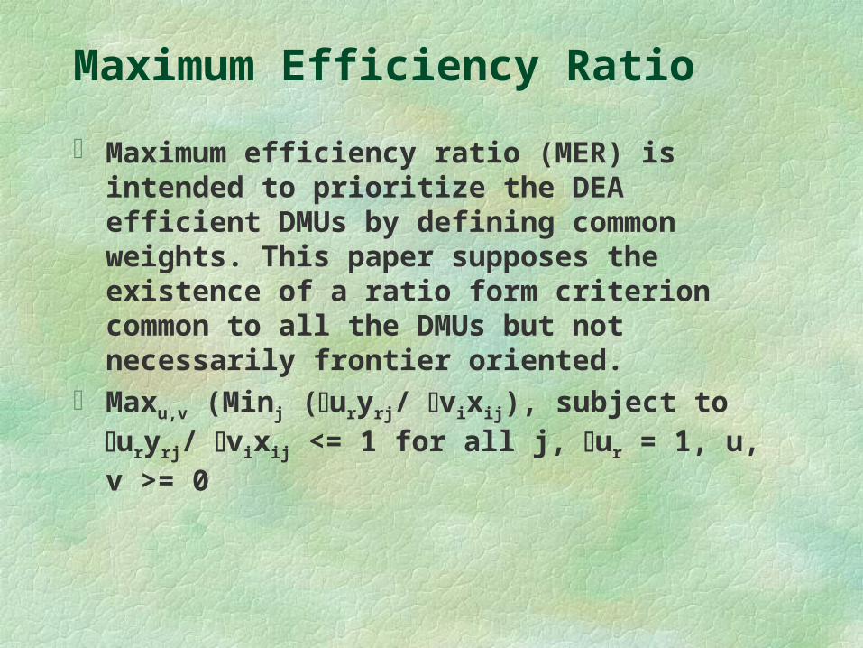
Maximum Efficiency Ratio
Maximum efficiency ratio (MER) is intended to prioritize the DEA efficient DMUs by defining common weights. This paper supposes the existence of a ratio form criterion common to all the DMUs but not necessarily frontier oriented.
Maxu,v (Minj (uryrj/ vixij), subject to uryrj/ vixij <= 1 for all j, ur = 1, u, v >= 0
Part IX: Computational Implementation
A Parallel and hierarchical decomposition approaches for solving large-scale Data Envelopment Analysis models
R.S. Barr and M.L. Durchholz

Part X: Abraham Charnes
Abraham Charnes remembered Abraham Charnes, 1917-1992 A bibliography for Data Envelopment Analysis (1978-
1996) LM. Setford

The End