Electrical Engineeringhttps://doi.org/10.1007/s00202-018-0723-7

ORIG INAL PAPER

Estimating power factor of induction motors at any loading conditionsusing support vector regression (SVR)

M. Khodapanah1 · A. F. Zobaa1 ·M. Abbod2

Received: 4 March 2017 / Accepted: 17 July 2018© The Author(s) 2018

AbstractThree-phase induction motors are industrial work horses known as inductive loads. Inductive loads always create low powerfactor due to consuming more reactive power. Low power factor not only makes a penalty charge for costumers, but alsoproduces energy losses in electrical systems. To prevent these problems, the power factor which is the ratio of active andreactive power must be maintained toward unity. The power factor can be controlled by manipulating either of active orreactive power. In induction motors, active power is proportional to the motor load that variation of motor load results inincrease or decrease in power factor. However, adding reactive power by capacitors would be a substantial solution to improveand control the power factor in unity. Many researches expressed that injecting improper reactive power to improve the powerfactor creates under- and over-correction. To prevent such problems, equation of power factor correction can be employed inorder to obtain the optimal value of reactive power. In this equation, the presence of power factor at every single loading pointis required. Estimation techniques can be a significant key to determine the power factor at every loading point. In this paper,several statistical methods including, kriging, regression, artificial neural network and support vector regression, are tested inthree induction motors. A comparison is presented to verify the great performance of support vector regression method.

Keywords Induction motors · PF · MCMD · Kriging · Regression · ANN · SVR

1 Introduction

Three-phase induction motors (IMs) are the main industrialwork horses that consume both active and reactive power [1,2]. IMs are known inductive loads that produce a high powerquality problem in electrical systems [3]. Inductive loads con-sume more reactive power. Consuming more reactive powerin loads such as IMs creates energy loss and voltage dropin the electrical systems [4]. To reduce the energy loss andvoltage drop, PF of IMs which is the ratio of active and reac-tive power must be maintained toward unity [5, 6]. In IMs,

B M. KhodapanahMohammadali.khodapanah@brunel.ac.k

A. F. Zobaaazobaa@ieee.org

M. AbbodMaysam.abbod@brunel.ac.uk

1 Department of Electronic and Computer Engineering, BrunelUniversity London, Uxbridge, UK

2 Department of Electrical Engineering, College ofEngineering, Brunel University London, Uxbridge, UK

the active and reactive power varies while the motor loadchanges from no-load to full-load that consequently PF willbe changed [7]. Bimbahara [8] described the reason that atno-load condition there is no mechanical resistance, the onlymagnetization reactance and motor resistance losses are pre-sented. The stator current will be divided in two componentsactive and reactive current in order to supply bothmechanicalresistance and magnetization reactance. Since the resistancelosses (friction and windage loss) are quit small, only a fewactive current pass through the resistance losses, but themajority of stator current as a reactive current flow inmagne-tization reactance and therefore the no-load current createshigh-angle legs the stator voltage in the range of 75°–85° [9].The stator PF at no-load will be approximately between 0.1and 0.3. However, as mechanical resistance increases, activecurrent or power increases gradually and flow in rotor sideto supply mechanical resistance. Then, it decreases the angleand improves the power factor in stator side about 0.8–0.9[9].

In industrial factories, many motor loads are changing oreven sometimes are working at light-load that causes low PF.The low PF in majority of IMs consuming more current is

123

Electrical Engineering

stored in the windage magnetic field and regenerated backto the grid line at each AC cycle [10, 11]. This exchangeis known reactive current which can be a cost factor. Toreduce this cost, generating reactive power is required inorder to improve low PF [12]. Capacitors bank is one of thesignificant solutions to generate reactive power and correctthe low PF. Obtaining the optimum value of required reac-tive power still is an unresolved challenge because in manycases the improper capacitors bank creates under- and over-correction in which under-correction produces low PF andover-correction causes self-excitation in IMs [13]. Presenceof PF at any loading condition can obtain the proper size ofcapacitors. The PF can be determined by the equivalent cir-cuit of IM that presents rotor and stator parameters. However,the equivalent circuit parameters need no-load test and lockrotor test that create a difficulty [2].

Many papers presented methods to determine the param-eters using measured data and other available informationfrommanufacturer data. For instance, Pedra [14], Haque [15]andMarcondes and Guimaraes [16] presented determinationof IM parameters from manufacturer data. Estimation of IMparameters with genetic algorithm is reported by Phumiphakand Chat-uthai [17]. However, by using the equivalent circuitmethod the value of PF can be obtained only at no-load andfull-load. In thismethod, to determine the PF at any loads, theslip or rotor speed requires that providing these parameterscan create a difficulty in measurement [18].

Ukil presented amethod usingmeasured current andman-ufacturer data (MCMD) to determine the PF of a small IM[9]. It also used the voltage and motor current measurementswith zero crossing method and instantaneous power methodto obtain the PF at any loads. In this method, the indicatedresults showed poor results particularly at large IMs due tovariation of reactive current. A normal meter device createsa difficulty to measure the PF at every single loading pointsdue to numerical fluctuation. Power analyzer can be used tomeasure and record the PF at every loading points to resolvethe reading issues. However, power analyzer not only is anexpensive device, but also is required the motor being switchoff for cable connection [19].

Therefore, estimation techniques would be an economicalsolution to predict the PF at every loading point. Hence, thesetechniques provide an online monitoring in order to enhancereliability and security of power quality in electrical sys-tems. In this research, several statistical methods with twocategories are used. Kriging and polynomial regression asnumerical techniques, artificial neural network (ANN) andsupport vector regression (SVR) as intelligent techniquesare used to estimate the PF of IM 100HP from no-load tofull/over-load conditions. Thesemethods required input data.The input values can be taken either from motor datasheet orby a few measurement points of voltage, current and inputpower from no-load to full-load conditions. In this paper, the

Fig. 1 Simulated IM by MATLAB/Simulink

estimated PF is compared with measured PF by simulationand practical work as well.

2 Case studies

In this study, a three-phase IM with range of 100HP is con-sidered from a stone cutting machine. The measurementprocedure took place when the operator moves the bladefor cutting the stone by variable volume gradually. A poweranalyzer named Uni power (UP-2210) is used to measureand record all components of three phases including volt-age, current, active and reactive power, PF and harmonics.The power analyzer stored all components in 6-min inter-val from no-load to full/over-load conditions. In addition, athree-phase IM in size of 100 HP with the same specificationof IM from industrial is modeled by MATLAB/Simulink.A torque meter is used to increase motor load step by step.Then, a simulated PF meter measures the PF from no-loadto full-load. The simulation diagram is shown in Fig. 1. Themeasured PF by power analyzer and simulation is illustratedin Fig. 2 in which the measured PF by simulation indicateda result close to the measured PF by power analyzer.

3 Kriging technique

Kriging is a geostatistical method, which is known as aninterpolation technique. The kriging estimates unknown val-ues based on nearby observed values at surrounding locationand weights them in order to minimize the error of a pre-dicted value. The kriging is more applicable in cases thatthe distance between each observed points and an unknownpoint is known. Therefore, the general kriging equation canbe expressed in Eq. (1).

Z(S0) �N∑

i�1

Wi Z(Si ) (1)

123

Electrical Engineering

Fig. 2 Measured PF by MATALB/Simulink

where Z(Si ) is the observed value at the i th location.Wi is anunknown weight for the observed value at the i th location.S0 is the prediction location. N is the number of observedvalues. To apply this equation, obtaining of weighs Wi areimportant in whichWi can be computed by a semivariogram.The semivariogram is a function that relates semivariance ofdata points. It also describes the spatial autocorrelation ofthe observed values. There are many semivariagram modelssuch as exponential, gaussian and spherical models. Expo-nential model, which can be a suitable for estimating PF, isapplied in this study. Therefore, the exponential function willbe expressed in Eq. (2)

γ (h) � c

(1 − exp

(−3h

a

))(2)

where c is sill that semivariance at which levelling takesplace, h is a distance between variables and a is a range thatrepresents the maximum distance in x-axis of semivariagrammodel. The important key point of this method is apply-ing a suitable semivariogram model to perform high outputaccuracy. Selecting the exponential model is more applica-ble since it is similar to the PF curve. Therefore, in Eq. (2),c can be replaced as a rated PF at maximum load (mPF), his a distance between all load points and a is replaced asa maximum load (mL). γ (i) is semivariagram of exponen-tial model. Lagrange matrix will be applied to obtain theweights of observed values. In the matrix, two main vectorsare needed. One is obtained values of semivariagram modelγ (i) and another is the distance between observed value andthe point that will be estimated. Then, the Lagrange multi-player matrix can be expressed in Eq. (3).

⎡

⎢⎢⎢⎢⎢⎣

W1

W2...Wn

λ

⎤

⎥⎥⎥⎥⎥⎦�

⎡

⎢⎢⎢⎢⎢⎣

γ11 γ12 · · · γ1n 1γ21 γ22 · · · γ2n 1...

.... . .

......

γm1 γm2 · · · γmn 11 1 · · · 1 0

⎤

⎥⎥⎥⎥⎥⎦

−1⎡

⎢⎢⎢⎢⎢⎣

γ10γ20...γn01

⎤

⎥⎥⎥⎥⎥⎦(3)

In Lagrange multiplication, Wi is (m ×1 matrix) theweight of actual and estimated points which is unknown, γiis (m ×n matrix) output of the semivariagram function andγno is a vector (m ×1) between the unknown loading pointsand observed loading points. Thus, from the obtaining val-ues of W1,W2, . . . ,Wn , the unknown PF can be estimatedby Eq. (4).

PF � W1F1 +W2F2 +WF3 + · · ·WnFn (4)

where Wi is a weight between an estimated point andobserved points and Fi is the observed PF. Then, multiplyingobserved points to obtained weights, PF at a desired point isgoing to be estimated. In the kriging algorithm, a loop func-tion has been applied in order to estimate the PF at any desiredloading condition [20, 21].

4 Regression technique

Regression analysis is a kind of statistical modeling thatuses to describe the relationships between the independentvariable x and the dependent variable y. Regression analy-sis is also applied to predict values named coefficients (βi )between a dependent variables (yi ) and independent variables(xi ).

Predicted coefficients (βi ) with independent variables (xi )create a new dependent variables (yi ) with a significantmodel. Least squares method which is more used of regres-sion analysis estimates the coefficients. There are manyfunctions to use in least squares method including poly-nomial, exponential, logarithmic and power. Among thesefunctions, polynomial function is more suitable in leastsquare methods because of providing a model by nth degrees[15]. The polynomial function can be expressed by Eqs. (5)and (6).

yi �n∑

i�1

f(xi,β

)+ εi (5)

yi � f (xi , β) � β0 + β1x1 + β2x22 + · · · + βmx

mn (6)

where in Eq. (5), yi is observed value. f(xi,β

)is a

polynomial function εi is error between observed and esti-mated values. In Eq. (6), (β0, β1, β2, . . . βm) are the coef-ficients of polynomial where m indicates the coefficients.(x1 + x22 + · · · xmn

)are independent variables where m and n

123

Electrical Engineering

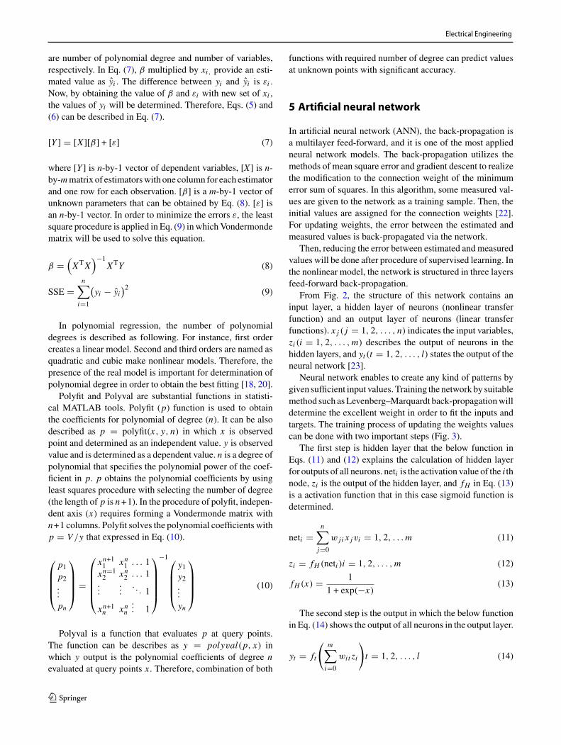
are number of polynomial degree and number of variables,respectively. In Eq. (7), β multiplied by xi, provide an esti-mated value as yi . The difference between yi and yi is εi .Now, by obtaining the value of β and εi with new set of xi ,the values of yi will be determined. Therefore, Eqs. (5) and(6) can be described in Eq. (7).

[Y ] � [X ][β] + [ε] (7)

where [Y ] is n-by-1 vector of dependent variables, [X] is n-by-mmatrix of estimatorswith one column for each estimatorand one row for each observation. [β] is a m-by-1 vector ofunknown parameters that can be obtained by Eq. (8). [ε] isan n-by-1 vector. In order to minimize the errors ε, the leastsquare procedure is applied in Eq. (9) in whichVondermondematrix will be used to solve this equation.

β �(XTX

)−1XTY (8)

SSE �n∑

i�1

(yi − yi

)2 (9)

In polynomial regression, the number of polynomialdegrees is described as following. For instance, first ordercreates a linear model. Second and third orders are named asquadratic and cubic make nonlinear models. Therefore, thepresence of the real model is important for determination ofpolynomial degree in order to obtain the best fitting [18, 20].

Polyfit and Polyval are substantial functions in statisti-cal MATLAB tools. Polyfit (p) function is used to obtainthe coefficients for polynomial of degree (n). It can be alsodescribed as p � polyfit(x, y, n) in which x is observedpoint and determined as an independent value. y is observedvalue and is determined as a dependent value. n is a degree ofpolynomial that specifies the polynomial power of the coef-ficient in p. p obtains the polynomial coefficients by usingleast squares procedure with selecting the number of degree(the length of p is n+1). In the procedure of polyfit, indepen-dent axis (x) requires forming a Vondermonde matrix withn+1 columns. Polyfit solves the polynomial coefficients withp � V /y that expressed in Eq. (10).

⎛

⎜⎜⎜⎝

p1p2...pn

⎞

⎟⎟⎟⎠ �

⎛

⎜⎜⎜⎜⎝

xn+11 xn1 . . . 1xn�12 xn2 . . . 1...

.... . . 1

xn+1n xnn... 1

⎞

⎟⎟⎟⎟⎠

−1⎛

⎜⎜⎜⎝

y1y2...yn

⎞

⎟⎟⎟⎠ (10)

Polyval is a function that evaluates p at query points.The function can be describes as y � polyval(p, x) inwhich y output is the polynomial coefficients of degree nevaluated at query points x . Therefore, combination of both

functions with required number of degree can predict valuesat unknown points with significant accuracy.

5 Artificial neural network

In artificial neural network (ANN), the back-propagation isa multilayer feed-forward, and it is one of the most appliedneural network models. The back-propagation utilizes themethods of mean square error and gradient descent to realizethe modification to the connection weight of the minimumerror sum of squares. In this algorithm, some measured val-ues are given to the network as a training sample. Then, theinitial values are assigned for the connection weights [22].For updating weights, the error between the estimated andmeasured values is back-propagated via the network.

Then, reducing the error between estimated and measuredvalues will be done after procedure of supervised learning. Inthe nonlinear model, the network is structured in three layersfeed-forward back-propagation.

From Fig. 2, the structure of this network contains aninput layer, a hidden layer of neurons (nonlinear transferfunction) and an output layer of neurons (linear transferfunctions). x j ( j � 1, 2, . . . , n) indicates the input variables,zi (i � 1, 2, . . . ,m) describes the output of neurons in thehidden layers, and yt (t � 1, 2, . . . , l) states the output of theneural network [23].

Neural network enables to create any kind of patterns bygiven sufficient input values. Training the network by suitablemethod such asLevenberg–Marquardt back-propagationwilldetermine the excellent weight in order to fit the inputs andtargets. The training process of updating the weights valuescan be done with two important steps (Fig. 3).

The first step is hidden layer that the below function inEqs. (11) and (12) explains the calculation of hidden layerfor outputs of all neurons. neti is the activation value of the i thnode, zi is the output of the hidden layer, and fH in Eq. (13)is a activation function that in this case sigmoid function isdetermined.

neti �n∑

j�0

w j i x jvi � 1, 2, . . .m (11)

zi � fH (neti )i � 1, 2, . . . ,m (12)

fH (x) � 1

1 + exp(−x)(13)

The second step is the output in which the below functionin Eq. (14) shows the output of all neurons in the output layer.

yt � ft

(m∑

i�0

wi t zi

)t � 1, 2, . . . , l (14)

123

Electrical Engineering

Fig. 3 Structure of NNBP layers. (Reproduced with permission from[23])

where ( ft (t � 1, 2, . . . , l) is a line function. The weightsset with observed values and are minimized by the delta ruleaccording to the learning samples. The topology in this studydetermines by a set of observed values and errors in order toselect the suitable number of neurons.

6 Support vector regression

The theory of SVR was developed by Vapnik in 1997 and isknown as one of the significant technique in terms of solvingregression problem. The SVR method constructs a hyper-plane in high-dimensional space in order to minimize thegeneralization error between defined upper and lower bound[24]. SVR can only act in linear way but bymapping themainspace into the higher-dimensional space, it would constructa set of hyperplanes close to the all data points to solve anonlinear model. The data point is D � {

Xi , ti }ni where xiis the input vector, ti is the target output and n is the num-ber of data sample. Therefore, the regression function can beexpressed in Eq. (15).

Y � f (x) � wφ(x) + b (15)

where φ(x) is the hyperplane in high-dimensional space. Xis a m-dimensional feature space. w and b are coefficients ofSVR that solve the regression problem. w and b are requiredto be found by minimizing the regularized empirical riskfunction in Eq. (16) and a loss function in Eq. (17).

Fig. 4 Error ε and limits ξ in the ε-insensitive function. (Reproducedwith permission from [25])

Remp � C1

n

n∑

i�1

Lε(ti , yi ) +1

2wTw (16)

Lε(ti − yi ) �{0 |ti − yi | ≤ ε

|ti − yi | − ε otherewise(17)

In the risk function, C 1n

∑ni�1 Ls(ti , yi ) is empirical risk

error and 12w

Tw is a regularization term or the flatnessof the function that needs to be minimized for simplifica-tion of the model. Lε(ti − yi ) is an intensive loss function.Parameter C is named as a capacity of the SVR that decidesthe trade between the regularization term and the empiricalrisk. E is named as size of the hyper-dimensional cylin-der that covers the function with the training data points.SVR performs linear regression in high-dimensional featurespace using ε-insensitive loss, and at the same time tries toreduce model complicity by minimizing wTw. The mini-mizationwould be determined by introducing slack variablesξ−i , ξ+i i � 1, . . . n since ε-insensitive loss is equal to slackvariables. Figure 4 indicates ε and limits ξ in the ε-insensitivefunction.

The parameters C and ε will be set by designer duringtraining step for optimizing slack variables [25]. To calculatethe parameters of w and b,, Eq. (16) changes to Eq. (17).Slack variables ξ−

i and ξ+i represent upper and lower limitsin the output and minimized by Eq. (18).

Minimize1

2wTw + C

n∑

i�1

(ξ−i + ξ+i

)

Subject to the constraints:⎧⎪⎪⎨

⎪⎪⎩

α+i −ti + yi + ε + ξ+i ≥ 0

α−i ti + yi + ε + ξ−

i ≥ 0μ+i ξ+i ≥ 0

μ−i ξ−

i ≥ 0

(18)

123

Electrical Engineering

where α+i , α−

i and μ+i , μ−

i are the coefficients of Lagrangemultipliers. The w will be obtained by applying partialderivative in Eq. (19).

∂R f

∂w� 0w �

∑

i

(α+i − α−

i )xi

∂R f

∂b� 0

∑

i

(α+i − α−

i ) � 0

∂R f

∂ξ+i� 0α+

i + μ+i � C

∂R f

∂ξ−i

� 0α−i + μ−

i � C (19)

Moreover, for obtaining the value of b, two main param-eters are required. One is w which is calculated by Eq. (19)and another is S (Support vector) that can be considered fromEq. (20). Therefore, considering both Eqs. (19) and (20), bwould be determined in Eq. (21). Therefore, regression func-tion in Eq. (22) solves the nonlinear problem.

S � {i | 0 < α+

i + α−i < C

}(20)

b � 1

|S|∑

i∈S

[ti − wT − xi − sign(α+

i − α−i )ε

](21)

y �∑

i

(α+i − α−

i )K(Xi , X j

)+ b (22)

where (α+i −α−

i ) is support vector coefficients and K(Xi , X j

)

is the kernel function. There are several kernel functions tosolve the minimization problem. In this study, radial basisfunction (RBF) using Gaussian is used by Eq. (23) where σ

is the dispersion coefficient of the Gaussian.

K(Xi , X j

) � exp

(− 1

2σ 2

∥∥Xi − X j∥∥)

(23)

In Lagrange multipliers, the following Karush–Kuhn—Tucker (KKT) and the quadratic programming will considernonzero values to the α+

i , α−i which are defined support

vectors. By multiplying the support vectors to the kernelK (Xi , X), the output provide errors equal, less or greaterthan ε. Kernel function is equal to vectors Xi and X j inthe feature space as φ(Xi ) and φ

(X j

)where K

(Xi , X j

) �φ(Xi )∗φ

(X j

). Therefore, the training of the SVR can solve

a quadratic and convex optimization problem [25].

7 Results and discussions

Input power measurement method is applied for motor loadcalculation in order to indicate PF against motor load. Deter-mining the PF at any load points leads to select the proper sizeof capacitors in order to prevent under- or over-correction.

Fig. 5 Results of estimated PF by MCMD method

Under-correction indicates low PF that produces a penaltyof charge. Over-correction generates more reactive power orcurrent than the motor needed. In such cases, self-excitationtakes place due to higher reactive current than magnetizingcurrent.

Hence, aforementioned reasons can prove the importanceof the PF fromno-load to full/over-load conditions. Ukil pub-lished a method using measured current and manufacturerdata (MCMD) to estimate the PF from no-load to full/over-load condition, and the result of IM 100HP in Fig. 5 showsthat the MCMD method produced hug errors from no-loadto full/over-load conditions in large IMs. This method onlyprovided satisfied performance in small IMs because in thesmall IM the reactive current is almost constant from no-loadto full/over-load.

However, the method was not able to estimate the PF inthe large IM because reactive current cannot be constantdue to high air gap that variation of motor loads from no-load to full/over-load causes reactive current to be changedhighly. In this paper, to resolve these issues, several estima-tion techniques have been implemented in order to minimizethe errors. Kriging and regression as numerical techniquesare used to estimate the PF. In Kriging, the distance betweentarget points and observed load points is considered. Then, byusing exponential function and Lagrange matrix, the weightof observed points is computed. Multiplying of observedpoints in their weights computed the PF at a desired point.In this method, a loop function is applied to predict the PFat every loading from no-load to full-load conditions. Theobtained weights times the observed PF provided the PF attarget load points.

Figure 6 indicated that Kriging generated results veryclose to the measured points from no-load to full-load. How-ever, it can be seen huge errors between estimated and

123

Electrical Engineering

Fig. 6 Results of estimated target PF by Kriging method

Fig. 7 Results of fitness in polynomial regression

measured values from full-load to over-load. Since Krig-ing is an interpolation technique, it is not able to make anextrapolation at over-load condition. However, in regression,polynomial function is applied in which polynomial degreesprovided significant roles that each number of polynomialdegree creates different models. Polyval and Polyfit in MAT-LABcanbe significant functions to determine thepolynomialcoefficients and then create a model fit to the observed PFcurve.

Figure 7 and Table 1 illustrated the trained data and pre-dicted polynomial coefficients in first, second, third andfourth orders. The evidence confirmed that polynomialregression with fourth order produced best fitting to theobserved PF curve. Therefore, based on the existed model,Fig. 8 indicates the estimated unknown PF from no-load to

Table 1 Predicted coefficients of polynomial degrees

Orders β1 β2 β3 β4 β5

Firstorder

0.0063 0.2498 – –

Secondorder

−9.1E−05 0.0173 −0.0121 –

Thirdorder

4.8E−07 −1.8E−04 0.0220 −0.079 –

Fourthorder

1.3E−08 −2.7E−06 8.7E−05 0.0133 0.0108

Fig. 8 Results of estimated PF in polynomial regression

full/over-load conditions. However, from full-load to over-load there is a huge gap between estimated and measuredPF. Although both methods produced results from no-loadto full-load very close to the measured points, kriging andregression methods could not fit the model in the over-loadcondition that results indicated extreme errors at over-loadcondition.

The reason is that both methods are not able to extrap-olate the data at unseen points. Figures 6 and 8 indicatedthat these methods obtained unacceptable results with hugeerrors at over-load conditions. To optimize these issues, thestudy found intelligent techniques including ANN and SVRin order to estimate the PF not only between the known obser-vation, but also to estimate the PF at over-load conditionswith high performance. In ANNmethod, feed-forward back-propagation algorithm is used inwhich five and three of inputdata are selected as training and testing, respectively. Con-sidering three hidden layer and a Levenberg–Marquardt totrain the algorithm indicated a significant generalization.

Figure 9 shows the fitness between observed points andoutput points where the output values are fitted to the inputdata. Figure 10 illustrates the estimated PF from no-load to

123

Electrical Engineering

Fig. 9 Results of fitness in NNBP

Fig. 10 Results of estimated PF in NNBP

full-load and over-load. The results illustrated that NNBPperformed a great fitting from no-load to over-load. In spiteof the fact that NNBP produced the results very close to mea-sured points with small error, several times are applied to runthe algorithm that each running generated different results.Therefore, in this method, obtaining the best result creates adifficulty due to running the algorithm more than once. Thiscan be a main disadvantage of ANN method. To optimizethe issue of NNBP, the SVR is used to provide a fixed modeland estimate the PF at any loading point. The strategy ofSVR is constructed a set of hyperplanes close to the all datapoints with a lower and upper bound. The RBF kernel func-tion is used to obtain the support vectors. The parameters ofSVR have a significant role in terms of creating a suitablemodel. In this case, the proper design of parameters indi-

Fig. 11 Results of estimated PF in SVR

Fig. 12 Results of fitness in SVR

cated a model very close to the observed points. The excitedmodel leads to estimate the unknown points from no-load tofull-load and over-load conditions properly. The estimatedPF from no-load to over-load points is shown in Fig. 11.As a result, the comparison between implemented methodsexpressed that the SVR method obtained satisfactory resultsin small, medium and large IMs. The possibility of adjustingthe parameters is one of the main advantages of this methodthat is able to provide desired models (Fig. 12).

The designed parameters of SVR are shown in Table 2.As a result, Table 3 illustrates the fitness and accuracy of

existed models where the fitness is computed by R-squaredand the accuracy obtained by minimum value divided bymaximum value at each points, and then the average value

123

Electrical Engineering

Table 2 Parameters of SVR Parameters Values

C 23

ξ 25

ε 0.00015

Table 3 Validity and accuracy of proposed methods

Methods Fitness R2 Error (%) Accuracy(%)

Computationtime (s)

Simulation – 2.946 96.864 0.032

MCMD – 14.448 85.552 0.005

Kriging – 1.681 98.319 0.015

PR firstorder

0.8855 9.749 91.454 0.047

PR secondorder

0.9975 2.036 97.971 0.043

PR thirdorder

0.9993 0.860 99.150 0.046

PR fourthorder

0.9999 0.932 99.104 0.048

ANN 0.9997 0.364 99.443 0.370

SVR 0.9999 0.348 99.653 0.272

provided accuracy. Error of estimated points is obtained bymean absolute percentage error (MAPE). In Kriging andMCMD, the input data are not trained as like as other meth-ods due to different strategies. The error results observedthat MCMD produced a lower accuracy in 85.5%. However,the SVR provided a high accuracy in 99.6% compared withothers. The error is calculated by mean absolute percentageerror (MAPE) which is shown in. The computation time inproposed methods are illustrated in second.

8 Conclusions

The power factor of induction motors is one of the signif-icant elements that must be maintained toward unity. Thepower factor is variable while the motor load changes fromno-load to full/over-load. This variation caused monitoringand determining the low power factor at any loading condi-tion becomes important due to finding the optimal reactivepower for power factor compensation. In this paper, severalestimation techniques are applied to estimate the power fac-tor at any loading conditions. Kriging and regression whichare numerical methods estimated the power factor with rea-sonable results from no-load to full-load. However, bothmethods produced very poor results from full-load to over-load. Neural network and support vector regression whichare intelligent techniques created greater results from no-load to full/over-load conditions in which the support vector

regression method indicated a satisfactory performance withaccurate results greater than ANN and numerical methods.

Open Access This article is distributed under the terms of the CreativeCommons Attribution 4.0 International License (http://creativecommons.org/licenses/by/4.0/), which permits unrestricted use, distribution,and reproduction in any medium, provided you give appropriate creditto the original author(s) and the source, provide a link to the CreativeCommons license, and indicate if changes were made.

References

1. Fuchs EF (2008) Power quality in power systems and electricalmachines. Academic Press, Cambridge

2. ChapmanS (2004)Electricmachinery fundamentals.McGraw-HillEducation, New York

3. Orsag P (2014) Impact of mains power quality on operation char-acteristics of induction motor. In: 14th international conference onenvironment and electrical engineering (EEEIC), 10–12May 2014,Ostrava, Czech Republic

4. Zahir J (2009) Estimation of power factor by the analysis of powerquality data for voltage unbalance. In: ICEE, Melborne

5. Kumar CP, Sabberwal SP, Mukharji AK (1994) Power factormeasurement and correction techniques. Electric Power Syst Res32:141–143

6. Guo L, Cheng Y, Zhang L, Huang H (2008) Research on power-factor regulating tariff standard. In: Proc. 2008 IEEE electricitydistribution conf., pp 1–5

7. Lalotra J (2016) Examination of the change in the power factor dueto loading effect. Int Res J Adv Eng Sci 1(1):25–28

8. Bimbhra P (1997) Electrical machinery. Khanna, Delhi9. Ukil A, Bloch R, Andenna A (2011) Estimation of induction motor

operating power factor from measured current and manufacturerdata. IEEE Trans Energy Convers 26(2):699–706

10. Khanchi S (2013) Power factor improvement of induction motorby using capacitors. Int J Eng Trends Technol 4(7):2967–2971

11. Ermis M (2003) Self-excitation of induction motors compensatedby permanently connected capacitors and recommendations forIEEE Std 141-1993. IEEE Trans Ind Appl 39(2):313–324

12. Adisa A (2006) A study of improving the power factor of a three-phase induction motor using static switched capacitor. In: Powerelectronics and motion control conference

13. Jimoh AA (2006) A study of improving the power factor of a three-phase induction motor using a static switched capacitor. In: 12thInternational power electronics and motion control conference,Pretoria North, South Africa 30 Aug–1 Sep 2006, pp 1088–1093

14. Pedra J (2008) On the determination of inductionmotor parametersfrom manufacturer data for electromagnetic transient programs.IEEE Trans Power Syst 23(4):1709–1718

15. Haque MH (2008) Determination of NEMA design inductionmotor parameters from manufacturer data. IEEE Trans EnergyConvers 23(4):997–1004

16. Marcondes J, Guimaraes C (2014) Parameter determination ofasynchronous machines frommanufacturer data sheet. IEEE TransEnergy Convers 29(3):689–697

17. Phumiphak T, Chat-uthai C (2002) Estimation of induction motorparameters based on field test coupled with genetic algorithm. IntConf Power Syst 2:1199–1203

18. OrmanM(2011) Slip estimation of a large inductionmachine basedonMCSA. In: Diagnostics for electric machines, power electronicsand drives (SDEMPED), 5–8 Sept. 2011

19. Khodapanah M, Zobaa AF, Abbod M (2016) Estimating powerfactor of induction motors using regression techniques. In: 17th

123

Electrical Engineering

International conference on harmonics and quality of power(ICHQP), Belohorizento, Brezil, Oct 16–19, 2016, pp 502–507

20. Khodapanah M, Zobaa AF, Abbod M (2015) Monitoring ofpower factor for induction machine using estimation technique.In 2015 50th international universities power engineering confer-ence, UPEC 2015, Stoke on Trent, United Kingdom, September1–4, 2015, pp 1–5

21. Guntaka R (2014) Regression and Kriging analysis for grid powerfactor estimation. J Electr Syst Inf Technol 1:223–233

22. Sagiroglu S (2006) Power factor correction technique based onartificial neural networks. Energy Convers Manag 47:3204–3215

23. Al-hnaity B (2015) Predicting FTSE 100 close price using hybridmodel. In: SAI intelligent systems conference (IntelliSys), 10–11Nov. 2015, London, UK, pp 49–54

24. Smola A (2004) A tutorial on support vector regression. Stat Com-put 14(4):199–222

25. Villazana S (2006) A novel method to estimate the rotor resistanceof the induction motor using support vector machines. In: IEEEindustrial electronics

Publisher’s Note Springer Nature remains neutral with regard to juris-dictional claims in published maps and institutional affiliations.

123