1

Transmission Loss Predictions for Dissipative Silencers of

Arbitrary Cross-Section in the Presence of Mean Flow

Ray Kirby

Department of Mechanical Engineering, Brunel University,

Uxbridge, Middlesex, UB8 3PH, UK.

2

Abstract

A numerical technique is developed for the analysis of dissipative silencers of arbitrary, but

axially uniform, cross section. Mean gas flow is included in a central airway which is

separated from a bulk reacting porous material by a concentric perforate screen. The analysis

begins by employing the finite element method to extract the eigenvalues and associated

eigenvectors for a silencer of infinite length. Point collocation is then used to match the

expanded acoustic pressure and velocity fields in the silencer chamber to those in the inlet

and outlet pipes. Transmission loss predictions are compared with experimental

measurements taken for two automotive dissipative silencers with elliptical cross sections.

Good agreement between prediction and experiment is observed both without mean flow and

for a mean flow Mach number of 0.15. It is demonstrated also that the technique presented

offers a considerable reduction in computational expenditure when compared to a three

dimensional finite element analysis.

3

I. INTRODUCTION

Dissipative silencers are effective for attenuating broad-band noise and are commonly

deployed in automotive exhaust and HVAC systems. A dissipative silencer often takes on a

complex geometrical shape, for example in an automotive exhaust system elliptic cross-

sections are common. Modelling complex silencer geometries presents a considerable

challenge, especially if one assumes the porous material to be bulk reacting. Inevitably,

numerical techniques have found favour for modelling irregular geometries and for

dissipative silencers the finite element method (FEM) is used widely. A general application

of the FEM to dissipative silencer design was presented by Peat and Rathi,1 who reported

transmission loss predictions for two axisymmetric exhaust silencers, both with and without

mean flow in the central airway. The analysis of Peat and Rathi is capable of modelling fully

arbitrary silencer geometries, although, in general, this requires the use of a three dimensional

finite element mesh2. Most silencer geometries are not, however, always of a fully arbitrary

shape; in fact, most dissipative silencers usually contain an axially uniform cross section. For

such a silencer it is desirable to take advantage of the uniform geometry and to avoid the

significant CPU expenditure associated with a three dimensional finite element model. One

possible solution is to apply the so-called point collocation technique suggested by Astley et

al.3 This method is versatile enough to cope with an arbitrary cross-section but also promises

to economise on CPU expenditure when compared to the method of Peat and Rathi1.

The model reported here examines a “straight-through” dissipative silencer containing an

axially uniform, but arbitrarily shaped, cross section. The model includes mean flow in the

central airway and also a perforated screen, separating the porous material from the central

airway, since this has been shown also to influence silencer performance.4 A uniform

4

silencer facilitates the reduction of the problem from three to two dimensions and in the

process potentially reduces CPU expenditure. Thus, the silencer chamber studied here is

assumed first to be infinite in length and an eigenvalue analysis is performed. Subsequently

the silencer transmission loss is computed by matching the expanded acoustic pressure and

velocity fields at the entry/exit planes of the silencer chamber.

The relative simplicity of an eigenvalue analysis, particularly when compared to a three-

dimensional approach, has meant that computing modal attenuation rates for dissipative

silencers has proved popular, although very few studies progress to calculating silencer

transmission loss. For example, Astley and Cummings5 use the FEM to compute modal

attenuation rates in dissipative silencers of rectangular cross-section, adding the effects of

mean flow in the central airway. The method of Astley and Cummings was later applied to

automotive silencer design by Rathi,6 who obtained modal attenuation rates for silencers of

an elliptic cross-section. Both studies do, however, omit the effects of a perforate and, more

importantly, neither progress to predicting the silencer transmission loss. A number of

alternative numerical eigenvalue formulations have also been sought for elliptical cross-

sections, examples include the Rayleigh Ritz approach of Cummings7 and the point matching

technique of Glav8. These alternative formulations do, however, compromise, to some

extent, the versatility and robustness of the FEM; the analysis of Cummings is restricted to

the fundamental mode only, the method of Glav is very sensitive to silencer geometry and the

collocation grid chosen. Moreover, Glav omits both mean flow and a perforate whilst

Cummings omits a perforate, and neither study progresses to computing silencer transmission

loss.

5

To predict silencer transmission loss, after first performing an eigenvalue analysis one begins

by expressing the acoustic pressure and velocity fields either side of a discontinuity (the inlet

and outlet planes in a uniform straight through silencer) as a modal expansion in which only

the modal amplitudes are unknown. These are then determined by matching acoustic

pressure and normal velocity across each discontinuity. This approach is commonly known

as mode matching and has been applied successfully to duct acoustics problems, for example,

Åbom9 implemented an analytic mode matching technique when modelling a reactive

exhaust silencer. In general, the method does, however, depend upon finding a transfer

matrix T for the silencer, whose elements ijt decay rapidly with increasing i, j. Without this

property the solution to the truncated system of matching conditions may bear little

resemblance to the solution of the physical problem. The decay of elements ijt largely

depends upon the weighting function chosen for the matching scheme. Åbom9 studied a

problem in which the underlying eigen-sub-system is Sturm-Liouville, thus, if one chooses

the modal eigenfunctions as weighting functions, modal orthogonality guarantees rapid decay

of elements ijt . The underlying eigen-sub-system for a dissipative silencer is, however, non

Sturm-Liouville and choosing the modal eigenfunctions as weighting functions does not

necessarily guarantee a convergent system of equations for a general class of problem. This

problem may be addressed by substituting a suitable orthogonality relation which, in effect,

restores modal orthogonality. Such an approach was adopted by Glav,10 who successfully

used an orthogonality relation to apply mode matching to a dissipative silencer of arbitrary

cross section. To arrive at a transfer matrix Glav utilises an appropriate orthogonality

relation which, crucially, is valid only for zero mean flow. To extend the approach of Glav to

include mean flow would require the solution of a system of equations in which the chosen

weighting function is not orthogonal. Of course the system of equations would remain

tractable however convergence to a solution characteristic of the physical problem may not

6

necessarily be achieved. This behaviour is apparent in the results of Cummings and Chang11

in which good agreement between prediction and experiment is observed, but only under

certain conditions, in this case at higher frequencies. At lower frequencies, when mean flow

is present, predictions do not tend towards zero transmission loss, as one would expect. It is

possible that this behaviour is caused by the absence of an orthogonality relation in the

analysis of Cummings and Chang11 when mean flow is present, and so the subsequent

solution bears little resemblance to the physical problem. In the absence of a suitable

orthogonality relation for the present class of problem, caution is therefore exercised and an

alternative method is investigated.

A straightforward alternative to analytic mode matching is to use a numerical matching

technique. The method of point collocation, implemented by Astley et al.3 in the study of air-

conditioning ducts, appears well suited to automotive silencer design. The technique

involves equating velocity and pressure fields at discrete points, or nodal locations, on the

cross section of the silencer, rather than integrating over the whole section as is the case when

matching analytically. Naturally, matching numerically cannot be expected to be as accurate

as matching analytically, however, with a suitable choice of collocation points Kirby and

Lawrie12 demonstrated that, for a rectangular duct lined on opposite walls, excellent

agreement with analytic mode matching predictions is possible. Although the study of Kirby

and Lawrie omitted mean flow, their results do appear to vindicate the application of point

collocation to the current problem. Of course, when implementing point collocation it is

convenient first to perform an eigenvalue analysis using the FEM. The collocation points,

over which pressure and velocity are matched, may then be chosen at any location over the

transverse cross section, although the number of collocation points must not exceed the

number of nodes in the original FE mesh. Thus, the analysis presented here first implements

7

a finite element eigenvalue analysis, based on the method of Astley and Cummings5 (with the

addition of a perforated screen), and then implements a numerical point collocation matching

scheme. Predictions are compared with experimental measurements taken for dissipative

exhaust silencers with elliptical cross sections.

II. GOVERNING EQUATIONS

The dissipative silencer consists of a concentric perforated tube surrounded by an (isotropic)

porous material of arbitrary cross-section (see Fig. 1). The silencer chamber, which has a

length L, is assumed to be uniform along its length, the outer walls of which are assumed to

be rigid and impervious. The inlet and outlet pipes (regions 1R and 4R ) are identical, each

having a circular cross section with rigid, impervious, walls.

Prior to matching acoustic pressure and velocity at each axial discontinuity, an eigenvalue

analysis is required, both for the silencer chamber and for the inlet/outlet pipes. Finding the

eigenvalues and associated eigenvectors for the inlet/outlet pipes is straightforward so listed

below is the eigenvalue analysis for the chamber only.

A. Governing equations for the silencer chamber.

The acoustic wave equation in region R2 is given by

0

12

2

2

22

20

=′∇−′

ptD

pD

c, (1)

8

where 0c is the isentropic speed of sound, p′ is the acoustic pressure and t is time. For

regions 2 and 3 a coupled modal solution for an axial wavenumber λ is sought; thus the

sound pressure in region 2 is expanded in the form

) ( 22

0 ) ,() ; , ,( xktiezyptzyxp

λω −=′ , (2)

where )( 00 ck ω= is the wavenumber in region R2, 1−=i and ω is the radian frequency.

Substituting the assumed form for 2p′ into the governing wave equation gives

[ ] 01 222

0222

022 =−−+∇ pkpMkpyz λλ , (3)

where M is the mean flow Mach number in region R2 and yz∇ denotes a two dimensional

form of the Laplacian operator (y, z plane).

Similarly for region R3, if the sound pressure is expanded in the form

) ( 33

0 ) ,() ; , ,( xktiezyptzyxp

λω −=′ , (4)

the wave equation may be written as

( ) 0322

02

32 =+−∇ pkpyz λΓ , (5)

provided mean flow in this region is assumed to be negligible and Γ is the propagation

constant of the porous material.

9

The appropriate boundary conditions which link together regions R2 and R3 are continuity of

normal particle displacement and a pressure condition which takes into account the presence

of the perforate. It is convenient to write each boundary condition in terms of the acoustic

particle velocity; thus for continuity of displacement

( ) 3322 nunu ⋅−−=⋅ 1 λM on cS , (6)

and for pressure

33 nu ⋅=− ζρ 0023cpp cc on cS . (7)

Here, u is the acoustic velocity vector, n the outward unit normal vector, and cp is the

sound pressure on boundary cS (the perforate) either in region R2 or region R3. The

(dimensionless) acoustic impedance of the perforate is denoted by ζ and 0ρ is the mean

fluid density in region R2. The assumption of an infinitesimally thin perforate is implicit in

Eq. (7) and is valid because the thickness of the perforate is typically small when compared

to the overall dimensions of the silencer. Finally, for the outer wall of the silencer chamber

(surface 3S ), the normal pressure gradient is zero; thus

03 =⋅∇ 3npyz on 3S . (8)

B. Finite element discretization and derivation of eigenequation.

The acoustic pressure in the chamber is approximated by a trial solution of the form

JJ

pzyzypN

J

21

22 ) ,() ,(2

∑=

= ψ and JJ

pzyzypN

J

31

33 ) ,() ,(3

∑=

= ψ (9a, b)

10

for regions R2 and R3 respectively. Here ) ,( zyJψ is a global basis function, Jp is the value

of z) ,(yp at node J, and 2N and 3N are the number of nodes in regions R2 and R3,

respectively. To arrive at the governing eigenequation the weak Galerkin method is adopted

and so for region R2 the wave equation may be re-written as

[ ][ ] 0 1

2

222

0222

022 =−−+∇∫

R

Iyz dydzpkpMkp ψλλ , for nodes 2,....,1 NI = . (10)

Applying Green’s theorem to equation (10) yields

[ ][ ] ∫∫ ⋅∇=−−+∇∇

22

2222

0222

02 1 CS

I

R

IIyzIyz dspdydzpkpMkp 2nψψλψλψ , (11)

where 2cS denotes the surface of the perforated tube which lies in region R2 and s is an

element length on surface cS . Substituting the assumed trial solution for 2p [Eq. (9a)] into

Eq. (11) gives

[ ]( )[ ] ∫∫ ⋅∇=

−−+∇∇

22

2222

0 1

CS

yzI

R

JIJyzIyz dspdydzMk 22 np ψψψλλψψ . (12)

Similarly, the weak Galerkin method allows the wave equation in region R3 to be written as

( )[ ] ∫∫ ⋅∇=

++∇∇

33

33322

02

CS

yzI

R

JIJyzIyz dspdydzk np ψψψλΓψψ , (13)

11

after utilising the pressure boundary condition on surface 3S [Eq. (8)]. Here 3cS denotes the

surface of the perforated tube which lies in region 3.

The final eigenequation for the chamber is obtained by using the boundary conditions on the

surface cS to couple together Eqs. (12) and (13). To facilitate the introduction of the

pressure and displacement boundary conditions it is necessary first to write the linearised

Euler equation, which for regions R2 and R3 gives

( ) 2u 102 λωρ Mipyz −−=∇ and 33 )( uωωρipyz −=∇ , (14a, b)

where )(ωρ is the equivalent complex density of the porous material (see Allard and

Champoux13). By substituting Eq. (14a) into the right hand side of Eq. (12), the displacement

boundary condition [Eq. (6)] may be introduced, giving

[ ]( )[ ] [ ] ∫∫ ⋅−=

−−+∇∇

22

32

0222

0 1 1

CS

I

R

JIJyzIyz dsMidydzMk nup 32 ψλωρψψλλψψ . (15)

For region 3, substitution of Eq. (14b) into the right hand side of Eq. (13) yields

( )[ ] ∫∫ ⋅−=

++∇∇

33

3322

02 )(

CS

I

R

JIJyzIyz dsidydzk nup 3ψωωρψψλΓψψ . (16)

The pressure boundary condition [Eq. (7)] may now be substituted into the right-hand side of

both Eqs. (15) and (16) to yield two equations which may then be combined to give a single

eigenequation of the form

12

[ ]( )[ ] +

−−+∇∇∫ 2p

2

1 2220

R

JIJyzIyz dydzMk ψψλλψψ

( )[ ] 322

02

3

p

++∇∇∫

R

JIJyzIyz dydzk ψψλΓψψ

[ ] 0)(

12

3

2

20

020 =−

+−

−− ∫∫ CCCC pppp

33

CC S

JI

S

JI dsk

idsMk

i ψψρ

ωρ

ζψψλ

ζ. (17)

Equation (17) constitutes a second order eigenvalue problem in λ . It is noticeable that the

order of this eigenequation has been reduced by 2 when compared to a similar study by

Astley and Cummings5, who omitted the perforate. Re-writing equation (17) in matrix form,

and re-arranging into ascending orders of λ , gives

[ ] ][][][ 2 0pCBA =++ λλ , (18)

where p is a vector accommodating the pressure in both regions 2 and 3. The matrices ][A ,

][B and ][C are given by

[ ] [ ] [ ] [ ] [ ] 22 CC2222 pMpMpKpMpKpA

ζΓ 0

332

3320][

ikk +++−=

[ ] [ ] [ ] 332 CCCCCC pMpMpM

323

0

00

0

0 )()(

ρ

ωρ

ζζρ

ωρ

ζ

ikikik+−− , (19)

[ ] [ ] [ ] 3

0020

222][ CCCC22 pMpMpMpB

222

ζζ

MikMikMk +−= , (20)

( )[ ] [ ] [ ] [ ] 32

20

202

022

0 1][ CCCC3322 pMpMpMpMpC22

ζζ

MikMikkMk −++−= , (21)

13

and

[ ] ∫ ∇∇=

2

,

R

JyzIyzJIdydzψψ2K (22a)

[ ] ∫ ∇∇=

3

,

R

JyzIyzJIdydzψψ3K (22b)

[ ] ∫=

2

,

R

JIJIdydzψψ2M (22c)

[ ] ∫=

3

,

R

JIJIdydzψψ3M (22d)

[ ] ∫=

2

,

CS

JIJIdsψψ

2CM (22e)

[ ] ∫=

3

3

,

CS

JIJIdsψψCM . (22f)

Finally, the problem may be solved for λ by re-writing Eq. (18) as

=

−− −−p

p

p

p

BCAC

I011 λ

λλ

][][][][

, (23)

where I is an identity matrix.

C. Numerical matching of sound fields.

Acoustic pressure and normal particle velocity are to be matched at collocation points on the

silencer inlet and exit planes, thus at plane A (see Fig. 1),

14

) , ,0() , ,0( 21 zyzy pp ′=′ , )or () ,( 12 RRzy ∈ , (24a)

) , ,0() , ,0(21

zyzy xx uu ′=′ , )or () ,( 12 RRzy ∈ , (24b)

) , ,0(03

zyxu′= , 3) ,( Rzy ∈ , (24c)

and for plane B,

) , ,() , ,( 42 zyLzyL pp ′=′ , )or () ,( 42 RRzy ∈ , (25a)

) , ,() , ,(42

zyLzyL xx uu ′=′ , )or () ,( 42 RRzy ∈ , (25b)

0) , ,(3

=′ zyLxu , 3) ,( Rzy ∈ , (25c)

where xu′ is the axial particle velocity. The acoustic pressure and velocity on either side of a

discontinuity are now written in terms of a modal expansion, containing both incident and

reflected waves. Prior to solving the problem, each modal expansion must be truncated

appropriately. Here the modal sum is truncated at the number of collocation points chosen

for an individual region. Thus, in region R1, if 1N collocation points are chosen, the sound

pressure may be expressed as

xikn

r

N

n

n

r

Mxik

ii

n

rePePzyx 1 01

1

0

11

)1(111 ) , ,(

λ−

=

+− ∑+=′ ΦΦp , )or () ,( 21 RRzy ∈ , (26)

where 1

1iP is the (known) modal amplitude in the inlet pipe, which is assumed here to contain

a plane incident wave only (hence 1iΦ is a unit vector of length 1N ). Here, the unknown

reflected modal amplitudes are denoted by n

rP1

, the (known) eigenvalues and associated

15

eigenvectors are denoted n

rλ 1 and n

rΦ respectively, where rΦ is a vector of length 1N . Thus,

the number of unknown modal amplitudes n

rP1

is equal to the number of collocation points in

region R1. Of course, on applying point collocation it is necessary to map the collocation

points in region R1 onto those in region R2, and so 21 NN = . Similarly for region 4,

xikn

i

N

n

n

i

niePzyx

′−

=

∑=′ 404

41

4 ) , ,( λΦp , )or () ,( 24 RRzy ∈ , (27)

assuming the outlet pipe is terminated anechoically downstream of plane B. Again, the

collocation points in region R4 should map onto those chosen in region R2, and so 42 NN = .

For the silencer chamber, the overall number of collocation points in regions R2 and R3 are

chosen as CNNN =+ 32 . Hence the modal expansion of the pressure field in the chamber is

given by

xikn

r

N

n

n

r

xikN

n

n

i

n

ic

n

cr

c

C

c

n

ci

C

ccePePzyx

λλ 00

11

) , ,(−

=

−

=

∑∑ +=′ ΨΨp , 32) ,( RRzy +∈ , (28)

where n

icP and n

rcP are the unknown modal amplitudes for the chamber. For the silencer

chamber, the eigenvalues n

icλ and n

rcλ , and the associated eigenvectors n

icΨ and n

rcΨ (each of

length CN ) are obtained on solution of Eq. (23). The modal expansions may now be

substituted into Eqs. (24) and (25), and the matching conditions enforced at each individual

node making up the transverse mesh, thus

16

11

1111

2

1 ii

n

r

N

n

n

r

n

i

N

n

n

i

n

r

N

n

n

r PPPPc

c

cc

c

cΦΨΨΦ −=−− ∑∑∑

===

, on 2R , (29a)

[ ] [ ] [ ]11

1111

2

1

1

1

111ii

N

nn

r

n

rn

r

n

r

N

nn

i

n

in

i

n

i

N

nn

r

n

rn

r

n

r PM

PM

PM

Pc

c

c

cc

c

c

c

ccΦΨΨΦ −=

−−

−−

−∑∑∑

=== λ

λ

λ

λ

λ

λ, on 2R , (29b)

011

=+∑∑==

c

ccc

c

ccc

N

n

n

r

n

r

n

r

N

n

n

i

n

i

n

i PP λλ ΨΨ , on 3R , (29c)

02

4

00

111

=−+ ∑∑∑==

−

=

−N

n

n

i

n

i

N

n

Likn

r

n

r

N

n

Likn

i

n

i PePePc n

cr

cc

c n

ci

ccΦΨΨ

λλ, on 2R , (29d)

[ ] [ ] [ ]0

111

2

1

1

4

00

111

=−

−−

+−

∑∑∑==

−

=

−N

n

n

in

i

n

in

i

N

n

Lik

n

r

n

rn

r

n

r

N

n

Lik

n

i

n

in

i

n

i

MPe

MPe

MP

c n

cr

c

c

cc

c n

ci

c

c

ccΦΨΨ

λ

λ

λ

λ

λ

λ λλ , on 2R (29e)

011

00 =+∑∑=

−

=

−c n

cr

ccc

c n

ci

ccc

N

n

Likn

r

n

r

n

r

N

n

Likn

i

n

i

n

i ePePλλ

λλ ΨΨ , on 3R . (29f)

This yields 32 24 NN + equations (the collocation points) and cNN 22 2 + ( 32 24 NN += )

unknown modal amplitudes, after putting 11

1=iP . Equations (29a)-(29f) may be solved

simultaneously to find the unknown modal amplitudes. Finally the sound transmission loss

of the silencer (TL) is given by11

1

4log 20 ipTL −= . (30)

17

III. EXPERIMENTAL TESTS

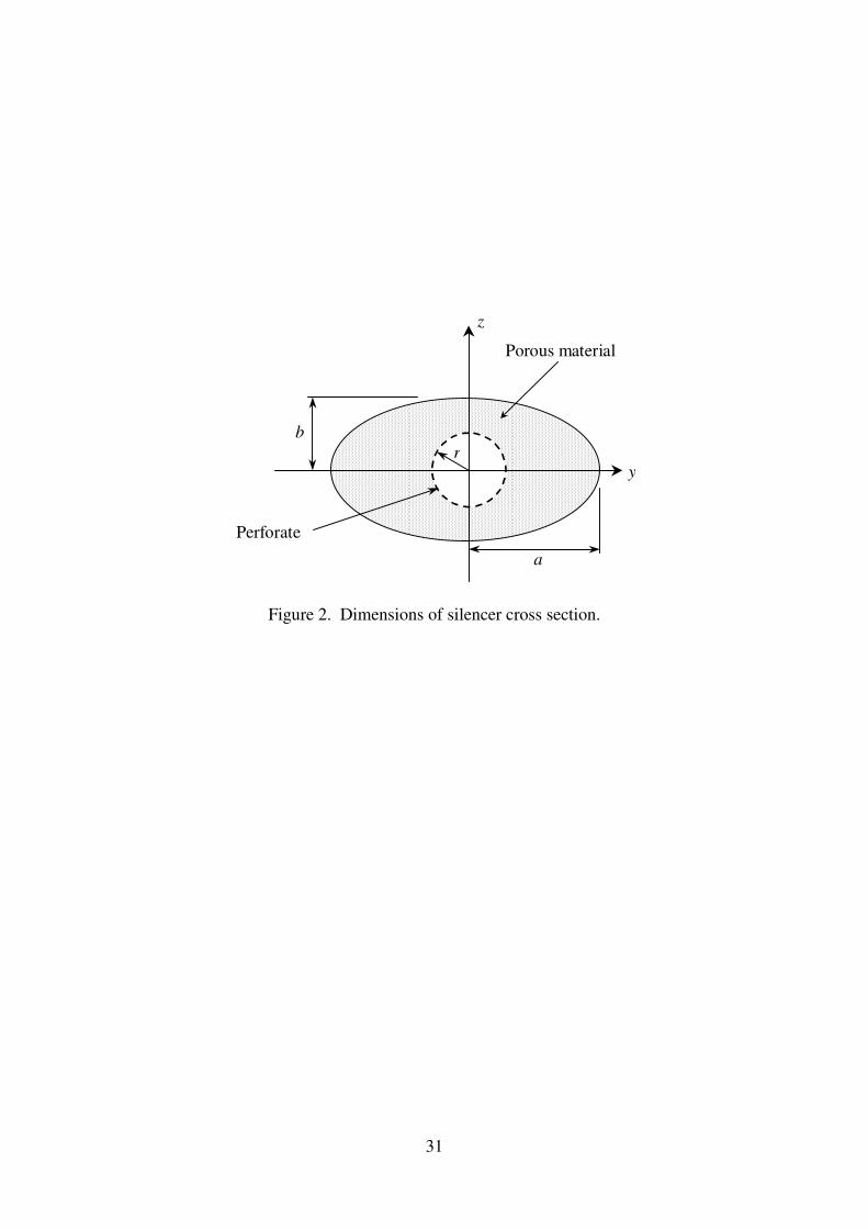
Experimental measurements were performed on two dissipative exhaust silencers, called here

silencer A and B. Each silencer is approximately elliptical in cross section and contains a

bulk reacting porous material separated from the central airway by a concentric perforated

screen (see Fig. 2). The chamber dimensions are summarised in Table I (for each silencer the

radius r of the perforated tube is 37 mm).

A. Silencer Transmission Loss.

The silencer transmission loss was measured using the impulse technique described by

Cummings and Chang11. This method is appropriate in the absence of an anechoic chamber

and is suited also to tests that involve mean fluid flow. The technique involves sending a

short rectangular pulse through the silencer and capturing the transmitted sound pressure.

The process is repeated after a suitable time interval and the transmitted sound pressure

successively averaged. The same procedure is followed after removal of the silencer from

the test rig and the transmission loss is computed by taking the logarithmic ratio of the two

captured average sound pressure spectra. A detailed account of the experimental technique is

given by the author in a paper on axisymmetric dissipative silencers,4 although it should be

noted here that the impulse technique inevitably incurs frequency limits outside of which

experimental measurements are inaccurate. At low frequencies, below approximately 150

Hz, erroneous measurements are common and these are caused largely by reflections from

the outlet test pipe arriving back at the silencer before all the reflections within the silencer

have died away. An upper frequency limit, approximately 1500 Hz here, is caused by a

18

significant roll-off in the pressure amplitude of the supplied pulse at frequencies above the

sampling frequency of 3 kHz.

B. Bulk Acoustic Properties of the Porous Materials.

Fibre glass and basalt wool are commonly used as acoustic absorbents in automotive

silencers. The fibre glass studied here is known commercially in the UK as E glass and has

an approximate average fibre diameter of 5-13 µm; the basalt wool studied here has a slightly

larger average fibre diameter of 6-18 µm. The analysis in Sec. II demands a knowledge of

the bulk complex density )(ωρ , and the propagation constant Γ for each porous material. It

is convenient here to write )(ωρ in terms of the (complex) characteristic impedance ( az ),

where ωΓωρ iza=)( (see Allard and Champoux13). The propagation constant and

characteristic impedance are specified here by combining the empirical power law approach

of Delany and Bazley14 with theoretical low frequency corrections. The semi-empirical

approach of Kirby and Cummings15 alleviates the non-physical predictions typically obtained

when applying Delany and Bazley power laws at low frequencies. For the materials studied

here, values for Γ and az were given by Kirby and Cummings as

( )[ ] ( )

( )[ ],

)(2iPr

1

21ln

3231ln211ln)(i

2

1

2200

0

2 2

4322

0

0

−

−−

++−

+++−++−=

ωπξ

Ω

γ

γ

ΩΩΩ

ΩΩΩΩΩΩΩωγ

Γ

sqq

k f

(31)

( )[ ] ( )

( )[ ],

)(2iPr

1

21ln

3231ln211ln)( 2

1

2200

0

2 2

432

20

2

00

−

−+

++−

+++−++−=

ωπξ

Ω

γ

γ

ΩΩΩ

ΩΩΩΩΩΩΩ

Ωγ

ω

ρ sq

q

c

z

f

a

(32)

19

where Ω is the porosity of the porous material, fξ is a dimensionless frequency parameter

( bf f σρξ 0= , where f is frequency and bσ is the flow resistivity of the bulk porous

material), 0γ is the ratio of specific heats for air, Pr is the Prandtl number, and 0q is the so-

called steady flow tortuosity. Kirby and Cummings define a “dynamic” tortuosity )(2 ωq and

shape factor )(2 ωs as

( )( ) ( )[ ] ( )[ ]( )[ ] ( ) 3231ln211ln

21ln 11)(

32

2271532

8264

ΩΩΩΩΩΩ

ΩΩΩξξξω

+++−++−

++−−++=

+aa

f

a

f

a

f aaaaq , (33)

( ) ( )[ ]48623751

20

22

11

1

2

)()(

af

a

f

a

faff aaaaq

qs

ξξξξπξ

ωω

+++= , (34)

where 81....aa are the Delany and Bazley coefficients measured experimentally.13 The

material constants measured for E glass and basalt wool are listed in Table II. Table II also

defines a transition value for fξ , denoted here 0f

ξ , below which )(2 ωq must be set equal to

20q in Eqs. (31) and (32) (see Kirby and Cummings15).

C. Acoustic Impedance of Perforate Screen.

The perforate screen used in each of the test silencers was constructed by forming a flat plate

with circular perforations into a concentric screen. The acoustic impedance of a perforated

plate was shown by Kirby and Cummings16 to increase when backed by a porous material.

They suggested the following semi-empirical relationship for the non-dimensional perforate

impedance )(ζ ,

20

+−′=

00

0

0.425i0.425

1

c

dzdk a

ρ

Γζ

σζ ,

(35)

where d is the diameter of the hole, σ is the area porosity of the perforate and ζ ′ is the

orifice impedance measured experimentally in the absence of a porous backing, and may be

written as χθζ i+=′ , where θ is the orifice resistance and χ the orifice reactance. In the

presence of mean flow Kirby and Cummings16 proposed the following empirical relationship

000

0

169.0

86537.02016.26 ckd

tdk

c

u

d

tνθ +−

−

= ∗

−

, (36)

where t is the thickness of the plate, ν is the kinematic viscosity of the mean gas flow, and

∗u is the friction velocity of the mean gas flow measured on the inner wall of the perforate.

The orifice reactance is given by ( )tk += δχ 0i , and Kirby and Cummings16 proposed

10

=δ

δ, tdftu 18.0≤∗ ,

dtdt

tdftu

d

t6.0

8.1

18.0exp6.01

0

−

+

−−

+= ∗

δ

δ, tdftu 18.0>∗ ,

(37)

and d849.00 =δ . When no mean flow is present, θ and χ were given by Bauer17 as

( ) 0081 ckdt νθ += , and ( )tdk += 25.0i 0χ . (38a, b)

21

IV. RESULTS AND DISCUSSION

The finite element mesh generated for both silencers A and B (see Table I) consisted of 6

noded triangular (in region 2R ) and 8 noded quadrilateral (in region 3R ) isoparametric

elements. For both silencers, 24 elements (88 nodes) were used to mesh the chamber, this

equates to 35 nodes in region 2R and 53 nodes in region 3R . Note that in order to implement

the pressure change boundary condition across the perforate [see Eq. (7)] it is necessary to

place a node on either side of the perforate and then to apply the boundary condition between

these two nodes. Thus, the finite element mesh includes two nodes (with identical

geometrical coordinates) at each nodal point along the boundary cS . For the inlet and outlet

pipes (regions 1R and 4R ) a mesh identical to the one in region 2R is used, this facilitates the

straightforward application of the point collocation matching technique. The silencer

transmission loss is calculated from Eq. (30) after first solving simultaneously Eqs. (29).

Transmission loss predictions are compared with experimental measurements in Figs. 3-6, for

silencers A and B with mean flow Mach numbers of 0=M and 15.0=M . Theoretical

predictions for 0=M were obtained by eliminating matrix ][B from Eq. (23) prior to

solution. For each silencer a concentric perforate screen of thickness mm 1=t , hole diameter

of mm 5.3=d and an open area porosity of 263.0=σ was used. When a mean flow Mach

number of 15.0=M is present, the friction velocity was measured to be m/s 56.2=∗u .

It is evident in Figs. 3-6 that good agreement generally exists between measured and

predicted silencer transmission loss. For frequencies below 1 kHz, predictions lie within

approximately 2 dB of measured values, although the transmission loss does tend to be over-

predicted. Above 1 kHz, a comparison with experiment is generally less successful and

22

differences of up to 6 dB are evident, largely for those measurements taken without mean

flow. Larger discrepancies at higher frequencies are, however, likely to be caused by

experimental error. Nevertheless, over the frequency range studied here, agreement between

prediction and experiment is deemed to be acceptable and is at least comparable in accuracy

to studies of dissipative silencers by other authors; see, for example, Cummings and Chang,11

Astley and Cummings,3 and Aurégan et al.18. Finally, the influence of the perforate is

examined in Figs. 7 and 8. Here a number of different values for perforate porosity are

examined for silencers A and B with a mean flow Mach number of 0.15. It is evident that, at

least for the silencers studied here, a small increase in transmission loss is obtained at low

frequencies when the perforate porosity is reduced, however, this is at the expense of a large

reduction in transmission loss at higher frequencies.

The computation of silencer transmission loss requires the inversion of three matrices: one of

order N2 (the inlet/outlet eigenvalues), one of order Nc (the chamber eigenvalues), and one of

order ( )cNN +22 (numerical matching). If one assumes a solver speed proportional to N3

then this CPU expenditure is generally higher than for an equivalent analytic matching

procedure. However, in the absence of a reliable analytic mode matching scheme when mean

flow is present, CPU expenditure compares favourably with the alternative fully three

dimensional treatment of Peat and Rathi1. For example, the method of Peat and Rathi was

applied to silencers A and B (see Table I) by Kirby2 (after omitting the perforate) and,

although generally good agreement between prediction and experiment was observed, the

three dimensional mesh required 1497 degrees of freedom for silencer A and 1757 for

silencer B. Thus for the silencers studied here point collocation represents a considerable

saving in CPU run time, amounting to approximately 99.5% for a solver whose speed is

proportional to N3.

23

The solution of Eq. (23) generates an unordered list of Nc incident and Nc reflected

eigenvalues and associated eigenvectors. The imaginary part of the incident and reflected

eigenmodes are then sorted into ascending order prior to the application of mode matching. It

is noticeable that, on solving Eq. (23) with mean flow present, so-called hydrodynamic

modes are not found. This is in contrast to a similar study by Astley and Cummings5 and is

caused by a change in the boundary condition between the airway and the porous material. In

the analysis presented here only transverse acoustic particle displacement across the perforate

is allowed. More importantly, transverse mean flow effects are suppressed at the perforate

that effectively prevents the formation of a fully free shear layer and serves to suppress the

generation of hydrodynamic modes. Of course, hydrodynamic modes have long been known

to exist when mean flow is present, and they are known to play an important role in the

performance of reactive silencers, however, when a porous material is present it is likely that

strong damping is provided by the material, and this will serve to reduce significantly the

influence of hydrodynamic modes on the sound pressure field. Thus, it is assumed in the

analysis presented in Sec. II, and the results presented here, that the acoustic performance of

the silencer is dominated by the behaviour of the least attenuated propagating modes and that

the effects of hydrodynamic modes may be neglected.

The transmission loss predictions shown in Figs. 3-8 were obtained after first establishing a

converged solution, that is, the number of collocation points were increased until the

variation in transmission loss was negligible over the frequency range shown. For

convenience, the collocation points were chosen to be identical to the nodal locations chosen

for the eigenvalue analysis, and so adaptation of the collocation points effectively takes place

prior to carrying out the eigenvalue analysis. Of course, so long as no more than Nc

24

collocation points are chosen, the collocation points need not be coincident with the nodal

locations in the original mesh. Moreover, in principle, it should be possible to reduce the size

of the collocation problem by reducing the number of collocation points to less than Nc.

However, as we do not know the shape of the final sound pressure field prior to numerical

matching, the choice of where best to put the collocation points becomes problematic,

especially at higher frequencies. The author has found the most reliable and robust approach

by choosing collocation points coincident in location with the nodes chosen for the

eigenvalue problem and to adapt the eigenvalue mesh only, i.e., to follow a standard finite

element adaptive procedure. Thus, for the current problem, matching is carried out over 35

collocation points in region R2, and 53 points in region R3 - collocation points equivalent in

number to the number of eigensolutions found in the silencer chamber. Of course, it is

widely known that for a finite element eigenvalue analysis one can rely on the accuracy only

of about 20% of the eigensolutions found. This does not present a problem here since the

sound pressure field at an individual collocation point is expressed as a modal sum [see Eqs.

(26)-(28)] and it is likely that, at least for the dissipative silencers studied here, the

performance of the silencer is dominated by the least attenuated modes, and these are the

modes which are found with the most accuracy using the FEM. For the current problem,

approximately 18 least attenuated modes may be deemed to be accurate and this number

should be more than sufficient to achieve a convergent sum in Eqs. (26)-(28), assuming that

hydrodynamic modes may be neglected. Thus, to solve the problem efficiently one needs

sufficient least attenuated modes to represent accurately the sound pressure field at an

individual collocation point, but also a sufficient number of points to accommodate the

variation in the transverse sound pressure field. For the current problem, 88 collocation

points are chosen in the chamber and, to maintain a square matrix and hence a tractable

problem, 88 eigenmodes are used in Eq. (28). On solving Eqs. (29) errors will therefore be

25

present in 80% of the modal amplitudes found, however these are amplitudes of highly

attenuated modes and so the effect on the overall silencer performance is negligible.

The transmission loss predictions presented in Figs. 3-8 cover a frequency range restricted by

experimental measurements. The technique presented here may, however, be used over a

much wider frequency range, provided the finite element mesh is adapted in the normal way.

This has been demonstrated by Kirby and Lawrie12 who successfully applied point

collocation to a relatively large HVAC silencer, although mean flow was omitted. Kirby and

Lawrie computed the transmission loss for a rectangular duct of cross-sectional dimensions

m 5.1m 5.1 × and lined on opposite walls with a bulk reacting material. Excellent agreement

between point collocation predictions and an exact analytic solution was reported for

frequencies up to 2 kHz, providing supporting evidence as to the accuracy of the current

method over a wider frequency range than the one presented here (based on a representative

ak0 value - "a" being a representative dimension of the duct).

IV. CONCLUSIONS

A finite length dissipative silencer of arbitrary, but uniform, cross section has been modelled

by combining a finite element eigenvalue analysis with a point collocation matching scheme.

The method is computationally efficient when compared to a three-dimensional finite

element approach and avoids the question of modal orthogonality. A good correlation

between prediction and experiment is observed both with and without mean flow, up to a

frequency of 1500 Hz for the silencers studied here, although in principle the method is

applicable over a much wider frequency range. Furthermore the flexibility and robustness of

the finite element method allows the technique to be applied to any cross sectional dissipative

26

silencer geometry, such as rectangular air conditioning ducts, and, in principle, to include any

number of duct discontinuities.

27

REFERENCES

1. K.S. Peat and K.L. Rathi, "A finite element analysis of the convected acoustic wave

motion in dissipative silencers," Journal of Sound and Vibration 184, 529-545 (1995).

2. R. Kirby, " The acoustic modelling of dissipative elements in automotive exhausts," PhD

Thesis, University of Hull, UK (1996).

3. R.J. Astley, A. Cummings and N. Sormaz, "A finite element scheme for acoustic

propagation in flexible-walled ducts with bulk-reacting liners, and comparison with

experiment," Journal of Sound and Vibration 150, 119-138 (1991).

4. R. Kirby, "Simplified techniques for predicting the transmission loss of a circular

dissipative silencer," Journal of Sound and Vibration 243, 403-426 (2001).

5. R.J. Astley and A. Cummings, "A finite element scheme for attenuation in ducts lined

with porous material: comparison with experiment," Journal of Sound and Vibration 116,

239-263 (1987).

6. K.L. Rathi, "Finite element acoustic analysis of absorption silencers with mean flow,"

PhD Thesis, Loughborough University, UK (1994).

7. A. Cummings, "A segmented Rayleigh-Ritz method for predicting sound transmission in

a dissipative exhaust silencer of arbitrary cross-section," Journal of Sound and Vibration

187, 23-37 (1995).

8. R. Glav, "The point-matching method on dissipative silencers of arbitrary cross section,"

Journal of Sound and Vibration 189, 123-135 (1996).

9. M. Åbom, "Derivation of four-pole parameters including higher order mode effects for

expansion chamber mufflers with extended inlet and outlet," Journal of Sound and

Vibration 137, 403-418 (1990).

28

10. R. Glav, "The transfer matrix for a dissipative silencer of arbitrary cross-section," Journal

of Sound and Vibration 236, 575-594 (2000).

11. A. Cummings and I.-J. Chang, "Sound attenuation of a finite length dissipative flow duct

silencer with internal mean flow in the absorbent," Journal of Sound and Vibration 127,

1-17 (1988).

12. R. Kirby and J.B. Lawrie "Modelling dissipative silencers in HVAC ducts," Proceedings

of the Institute of Acoustics Spring Conference, Salford University, Salford, UK., 24(2)

(2002).

13. J.F. Allard and Y. Champoux, "New empirical equations for sound propagation in rigid

frame fibrous materials," Journal of the Acoustical Society of America 91, 3346-3353

(1992).

14. M.E. Delany and E.N. Bazley, "Acoustical properties of fibrous materials," Applied

Acoustics 3, 105-116 (1970).

15. R. Kirby and A. Cummings, "Prediction of the bulk acoustic properties of fibrous

materials at low frequencies," Applied Acoustics 56, 101-125 (1999).

16. R. Kirby and A. Cummings, "The impedance of perforated plates subjected to grazing gas

flow and backed by porous media," Journal of Sound and Vibration 217, 619-636 (1998).

17. A.B. Bauer, "Impedance theory and measurements on porous acoustic liners," Journal of

Aircraft 14, 720-728 (1977).

18. Y. Aurégan, A. Debray and R. Starobinski, "Low frequency sound propagation in a

coaxial cylindrical duct: application to sudden area expansions and to dissipative

silencers," Journal of Sound and Vibration 243, 461-473 (2001).

29

Table I. Data for test silencers.

Silencer Major axis (a, mm)

Minor axis (b, mm)

Length (L, mm)

Porous material

A 110 60 350 Basalt Wool

B 95 50 450 E. Glass

Table II. Porous material constants.

Constant E glass Basal Wool

1a 0.2202 0.2178

2a -0.5850 -0.6051

3a 0.2010 0.1281

4a -0.5829 -0.6746

5a 0.0954 0.0599

6a -0.6687 -0.7664

7a 0.1689 0.1376

8a -0.5707 -0.6276

bσ (MKS rayl/m) 30716 13813

Ω 0.952 0.957

20q 5.49 2.91

0fξ 0.005 0.0079

30

Porous material

x

1R4R2R

3R

A B

x′

Perforate

y

z

2n

MachNumber M

2R

3R

3n

CS

3SL

Figure 1. Geometry of silencer.

31

Porous material

Perforate

y

z

a

b

r

Figure 2. Dimensions of silencer cross section.

32

Figure 3. Transmission loss for silencer A with 0=M . ——— experimental measurement;

— — — prediction.

0

10

20

30

40

50

0 500 1000 1500

Frequency (Hz)

Tra

nsm

issi

on L

oss

(dB

)

33

Figure 4. Transmission loss for silencer A with 15.0=M . ——— experimental

measurement; — — — prediction.

0

10

20

30

40

0 500 1000 1500

Frequency (Hz)

Tra

nsm

issi

on L

oss

(dB

)

34

Figure 5. Transmission loss for silencer B with 0=M . ——— experimental measurement;

— — — prediction.

0

10

20

30

40

50

0 500 1000 1500

Frequency (Hz)

Tra

nsm

issi

on L

oss

(dB

)

35

Figure 6. Transmission loss for silencer B with 15.0=M . ——— experimental

measurement; — — — prediction.

0

10

20

30

40

0 500 1000 1500

Frequency (Hz)

Tra

nsm

issi

on L

oss

(dB

)

36

Figure 7. Transmission loss predictions for silencer A with 15.0=M . — — — 5.0=σ ;

——— 263.0=σ ; — - — - — 1.0=σ ; — - - — - - — 05.0=σ .

0

10

20

30

40

0 500 1000 1500

Frequency (Hz)

Tra

nsm

issi

on L

oss

(dB

)

37

Figure 8. Transmission loss predictions for silencer B with 15.0=M . — — — 5.0=σ ;

——— 263.0=σ ; — - — - — 1.0=σ ; — - - — - - — 05.0=σ .

0

10

20

30

40

0 500 1000 1500

Frequency (Hz)

Tra

nsm

issi

on L

oss

(dB

)