ERASMUS UNIVERSITY ROTTERDAMErasmus School of Economics

Why are asset prices so volatile?Sales Growth Persistence and the Expectation Hypothesis

A thesis submitted in partial fulfilment of the requirements for the degree of Master of Science in

Econometrics and Management Science -Quantitative Finance

S.R. Herrewijn365982

Supervisor: Dr. R.J. Lange i

Second Assessor: S.H.L.C.G. Vermeulen

November 9, 2018

Abstract

Aiming to find the missing link between accounting numbers and stock return volatility, this paperexamines how sales growth persistence is related to Extrapolation Hypothesis via the variance of itsasset returns. Differentiating from the literature, growth persistence is captured by a mean-revertingstate space model. Portfolios formed on the level of growth persistence feature many favourableattributes. Within this framework high-persistent companies are found to realise high sales growthand show signs of predictability. Combining growth persistence, quarterly report announcementsand the forecast errors from the state space model as explanatory variables in the conditional vari-ance equation in a GARCH framework, the results show evidence that these variables add to theexplanation of realised volatility. The research forms evidence that suggest a difference in reactionto forecast errors along the growth persistence portfolios. Overall the findings of the study representa first step in the direction of applying company fundamentals in explaining stock return volatility.

Keywords: Sales Growth Persistence, State Space Modeling, Local Linear Mean-Reverting TrendModel, Expectation Hypothesis, GARCHX, Excess Volatility.

Contents

1 Introduction 1

2 Literature Review 82.1 Empirical Stock Prices and Cash Flows . . . . . . . . . . . . . . . . . . . . . . . . . . . . 92.2 Persistence Sales Growth . . . . . . . . . . . . . . . . . . . . . . . . . . . . . . . . . . . . 112.3 Modelling Stock Return Volatility . . . . . . . . . . . . . . . . . . . . . . . . . . . . . . . 122.4 Extrapolation Hypothesis . . . . . . . . . . . . . . . . . . . . . . . . . . . . . . . . . . . . 13

3 Data 15

4 State Space Modelling 194.1 General State Space Model . . . . . . . . . . . . . . . . . . . . . . . . . . . . . . . . . . . 194.2 Univariate Time Series Models . . . . . . . . . . . . . . . . . . . . . . . . . . . . . . . . . 204.3 Kalman Filter and Smoother . . . . . . . . . . . . . . . . . . . . . . . . . . . . . . . . . . 214.4 Parameter Estimation . . . . . . . . . . . . . . . . . . . . . . . . . . . . . . . . . . . . . . 22

5 Methodology 255.1 Persistence in sales growth . . . . . . . . . . . . . . . . . . . . . . . . . . . . . . . . . . . . 255.2 Extrapolation Hypothesis . . . . . . . . . . . . . . . . . . . . . . . . . . . . . . . . . . . . 30

6 Results 346.1 Persistence in Sales Growth . . . . . . . . . . . . . . . . . . . . . . . . . . . . . . . . . . . 346.2 Persistence in Earnings Growth . . . . . . . . . . . . . . . . . . . . . . . . . . . . . . . . . 426.3 Extrapolation Hypothesis . . . . . . . . . . . . . . . . . . . . . . . . . . . . . . . . . . . . 436.4 Case Study: Apple Inc. vs. Ford Motor Company . . . . . . . . . . . . . . . . . . . 49

7 Discussion and Conclusion 55

A Appendix A: Proofs and Derivations 66A.1 Derivation of the Kalman Filter and Smoother . . . . . . . . . . . . . . . . . . . . . . . . 66A.2 Derivation of the EM Algorithm . . . . . . . . . . . . . . . . . . . . . . . . . . . . . . . . 70A.3 Optimising Initial Values . . . . . . . . . . . . . . . . . . . . . . . . . . . . . . . . . . . . 74

B Appendix B: Tables 75

List of Tables

1 Number of Companies & Descriptive Statistics . . . . . . . . . . . . . . . . . . . . 16

2 Economy-wide Average Sales Estimated Parameters . . . . . . . . . . . . . . . . . 35

3 Formed Portfolios based on the Estimated ϕ . . . . . . . . . . . . . . . . . . . . . . 36

4 Annualised Sales Growth . . . . . . . . . . . . . . . . . . . . . . . . . . . . . . . . . . 38

5 Correlation between Returns Around Announcement Period t∗ . . . . . . . . . . 43

6 GARCH Optimal Model Preferences . . . . . . . . . . . . . . . . . . . . . . . . . . . 44

7 News Effect over the Different Portfolios . . . . . . . . . . . . . . . . . . . . . . . . 48

8 Case Study: Sales Growth Estimation Results . . . . . . . . . . . . . . . . . . . . . 49

9 Case Study: Fundamentals . . . . . . . . . . . . . . . . . . . . . . . . . . . . . . . . . 51

10 Case Study: GARCH Estimation Results . . . . . . . . . . . . . . . . . . . . . . . . 53

11 Case Study: News Effect . . . . . . . . . . . . . . . . . . . . . . . . . . . . . . . . . . 54

B.1 Portfolio Fundamentals . . . . . . . . . . . . . . . . . . . . . . . . . . . . . . . . . . . . 75

B.2 Annualised Return Rate . . . . . . . . . . . . . . . . . . . . . . . . . . . . . . . . . . . 77

List of Figures

1 Workflow Diagram: Relating Fundamentals to Stock Return Volatility . . . . . 5

2 Distribution of the Number of Companies . . . . . . . . . . . . . . . . . . . . . . . 15

3 Comparison between Realised Return and Volatility and Leading Indices. . . . 17

4 Persistence Model Overview . . . . . . . . . . . . . . . . . . . . . . . . . . . . . . . . 29

5 Economy-wide Average Estimated Sales Level, Growth, and Seasonality . . . . 35

6 Estimated Level of Growth Persistence, ϕ . . . . . . . . . . . . . . . . . . . . . . . . 36

7 Time Series of Excess Mean and Median Sales Growth . . . . . . . . . . . . . . . 39

8 Distribution over Industries and Corresponding Average Growth. . . . . . . . . 41

9 Correlation between Earnings Persistence and Sales Persistence . . . . . . . . . 42

10 GARCH Exogenous Parameter Distributions . . . . . . . . . . . . . . . . . . . . . 45

11 Optimal GARCH Models . . . . . . . . . . . . . . . . . . . . . . . . . . . . . . . . . . 46

12 Adjusted R2 of the Mincer-Zarnowitz Regression . . . . . . . . . . . . . . . . . . . 47

13 Case Study: Estimated Sales . . . . . . . . . . . . . . . . . . . . . . . . . . . . . . . . 50

14 Case Study: Return and Volatility . . . . . . . . . . . . . . . . . . . . . . . . . . . . 52

15 Case Study: GJR Series . . . . . . . . . . . . . . . . . . . . . . . . . . . . . . . . . . . 55

List of Abbreviations

General

ML Maximum LikelihoodEM Expectation Maximisation AlgorithmOLS Ordinary Least-SquaresAIC Akaike Information Criterion

Data

CRSP Centre for Research in Security PricesEPS Earnings-per-ShareDPS Dividends-per-ShareR&D Research and DevelopmentSIC Standard Industrial ClassificationGDP Gross Domestic ProductVIX Chicago Board Options Exchange Volatility IndexS&P500 Standard and Poor’s 500 Stock Market Index

State Space Modelling

BSTM Basic Structural Time Series ModelLLM Local Level ModelLLT Local Linear Trend ModelAR Auto-Regressive ModelWGS Weighted Average Rank of Sales GrowthNP Non-Persistent PortfolioLP Low-Persistent PortfolioHP High-Persistent Portfolio

Volatility Modelling

GARCH Generalised Auto-Regressive Conditional Heteroskedasticity ModelGJR Glosten-Jagannathan-Runkle ModelPEAD Post-Earnings-Announcement DriftSUR Earnings Surprise

List of Symbols

General

L Likelihood i Company` Log-Likelihood n Total number of companiesθ Parameter Set t Timep Probability Density Function T Final Time PointI Information Matrix

State Space Modelling

y Observation σ2ε Observation Variance

Z Design Vector µ Level-Componentα State Vector η Level DisturbanceΩ Observation Regression Coefficients σ2

η Level Varianced Exogenous Variable Observation Equation δ Trend-Componentε Observation Noise δ Average TrendH Observation Disturbances ζ Trend DisturbanceT Transition matrix σ2

ζ Trend Variance

Φ State Regression Coefficients τ Seasonal-Componentc Exogenous Variable State Equation υ Seasonal DisturbanceR Selection Matrix σ2

υ Seasonal Varianceη State Noise ϕ Trend Persistence ParameterQ State DisturbancesP State Estimation Forecast Error

q Number of Observed Dependent Variablesk Number of Exogenous Variables in the Observation Equationm Unobserved Latent States of the State Space Models Number of Exogenous Variables in the State Equationg Number of Error Terms Influencing the State EquationsS Number of Seasonal Components

Volatility Modelling

r Weekly Return a Mincer-Zarnowitz Regression Interceptψ Unconditional Average Weekly Return b Mincer-Zarnowitz Regression Parameter Estimateν Return Innovations e log Mincer-Zarnowitz Regression Interceptz White Noise process f log Mincer-Zarnowitz Regression Parameter Estimateh Time-Varying Conditional Variance v Disturbance of the Mincer-Zarnowitz Regressionω Unconditional Variance w Disturbance of the log Mincer-Zarnowitz Regressionλ Lagged Squared Innovations RV Realised Varianceβ Lagged Conditional Variance R2 Adjusted R2

γ Estimate Exogenous VariableX Exogenous Variable in the Variance Equation

1 Introduction

Will Apple’s, Facebook’s and Google’s revenues ever stop growing? Ever since they are listed on

the global stock markets, their market capitalisation and cash flows have grown tremendously, exceeding

every rational economic business valuation theory. At the bottom line lies the general assumption that

the present value of a company is the expectation about future cash flows at a certain discount rate.

This implies two fundamental questions: what would be a reasonable expectation about a company’s

upcoming cash flows and at which rate should it be discounted? The main body of financial literature

focuses on finding the fair present value of a company and therefore finding the perfect price of its assets.

Where forthcoming cash flows show persistence and forecastability, it is widely accepted that the asset

prices are best described by a random walk, show very little predictability and exhibit large (clustered)

disturbances. Hence rises the question: if the underlying cash flows are to some extent predictable, why

are the stock prices so utterly volatile?

Stock return volatility has been a major interest in both academic and business papers, of which

Engle (1982), Bollerslev (1986) and Andersen et al. (2001) where among the first to model the time

series properties of return volatility. French et al. (1987) and Campbell and Hentschel (1992) examined

the relation between asset returns and market volatility and Ang et al. (2006) created a profitable trading

strategy out of stock return volatility. The connection between a company’s stock return and its funda-

mental values originates from studies of Shiller (1981), Summers (1986) and Fama and French (1992),

from which the latter find two important risk factors in value and size. The association between cash

flows (dividends and earnings) and returns, finds a striking result in the study of Lamont (1998), who

shows evidence of predictive power of these cash flows for excess stock returns. Where most academia

focus on earnings and dividends as measure of operating performance, they largely overlook sales as

insightful fundamental number. As earnings are the main target of investors and financial analysts, they

are prompt to various methods of earnings management and/or based on unreliable accrual numbers,

making it doubtful estimate of actual operating performance (Richardson et al. (2005)). Sales or rev-

enue on the other hand is a much cleaner proxy of such performance. The preference of sales is further

supported by the work of Chan et al. (2003), who find that contrary to earnings, sales are more predict-

able, due to a greater level of persistence in growth rates and are overall less volatile (Kiger (1974)). It

therefore straightforward to relate persistent sales to excessively volatile stock returns. In particular it

is interesting to link if more sales persistence leads to less excessive return volatility.

This link splits the problem in two parts. First of all, how persistent is firm revenue growth? And

second, does high persistence result in less excess volatility? A partial solution finds its origin in the

1970 paper of Beaver et al. (1970), who were among the first to find a correlation between the variance of

1

the stock price and the volatility of cash flows. Later Campbell and Shiller (1988) show that stock price

volatility cannot only be caused by changes in expectations of future excess return. They decompose

the variance into two parts, expectations about returns and expectations about cash flows. Vuolteenaho

(2002) provides further evidence that, on a firm level, the largest part of the variance originates from

changes in expectations about cash flows rather than the actual level. In other words, the larger part of

the variance is caused by different interpretations about how the current state reflects into the expectation

of the upcoming cash flows.

Many previous studies that opt to evaluate the expectations of financial analysts conclude a large

heterogeneity among the these practitioners and many fail to provide accurate forecasts of upcoming cash

flows. As further shown by La Porta (1996) among others, analysts are excessively optimistic about past

winners and tend to extrapolate this recent winning streak too far into the future resulting in significant

negative portfolio returns. La Porta refers to this phenomenon as the Extrapolation Hypothesis, and

constructs portfolios based on their expected earnings growth, to obtain such counter-intuitive results.

In the follow-up study La Porta et al. (1997) find that investors actually overestimate the persistence in

growth rates and project periods of prolonged growth to far into the future, which has been in line with

the earlier study of Lakonishok et al. (1994).

To find the missing link between the persistence in sales growth and the excessive volatility found in

stock returns, I aim to find a specific relation between the Extrapolation Hypothesis on one side and the

volatility spike occurring at announcements of quarterly reports on the other. This problem statement

arose arguing over the hypothesis that if the sales growth is more persistent, investors would have a

rather good idea about what the expect regarding the next periods sales growth. This would indicate a

smaller volatility shock around a report announcement, than it would with a non-persistent growth rate.

If sales posses some level of persistence, which in the context of this thesis will be formulated as

the ability of a company to achieve sales growth that deviates for multiple periods from the economy-

wide average growth, they are to some extend predictable. This deviates from the definition used in

prior literature. By the definition of Fama and French (2002) and Chan et al. (2003), sales or earnings

persistence is defined as consecutive years of growth, concluding that in their empirical studies it is very

hard to find significant results. As an example, a firm that outperforms in the first and second year,

stagnates in the third consecutive year, and again realises excess growth in the next two years, would

be left out of the sample after the second year. Overall they conclude that sales growth can only be

endured over a short time period. Based on our definition, the previous example means a relative strong

persistence in sales growth over the past 5 years. Therefore using this alternative definition, I aim to

find a more complete view of the actual sales persistence. Nevertheless, sales growth persistence is still

a rare phenomenon, because on a firm level, sales growth reverts back to the economy average, which is

2

approximately equal to the growth of the gross domestic product (GDP) (Chan et al. (2003)). And so,

only a small fraction of companies is able to realise such continuous out performance.

In contrast to prior literature, this study analyses each individual company with univariate time series

techniques, resulting in a data set with both a time series dimension as well as dimension over a large set

of companies. So far however, studying growth rates ignored a large part of the companies’ time series

properties, whilst some time series research only investigates a small group of companies or a major stock

market index. This combination paves the way for clustering companies based unique characteristics and

additionally enables us to look at specific events in time or specific companies throughout a certain time

period.

Analysing such univariate time series opens the door to a wide range of models and methods. However,

finding persistence, mean-reversion and seasonality in sales growth rates drastically reduces the number

of suitable models. One of the most general time series models is the basic structural time series model

(BSTM) of Harvey (1990). This state space framework can be modified in such a way that it satisfies

all the defined features. The preference for the state space framework is primarily due to the ability

of estimating a trend without directly model the first differences. The main model of interest is the

local linear mean-reverting trend model (LLT), where in the trend equation I added a mean or average

growth rate, and a parameter of persistence, which allows the estimated trend to under- or outperform

the market average. The LLT model is an extension of a simpler version of BSTM models, a basic

local level model (LLM) which restricts the persistence parameter and growth variance at zero, resulting

in the addition of a deterministic growth term. As these two models use the sales level as input, one

might argue if the sales growth cannot be analysed directly. Therefore a third model intents to capture

persistence and mean-reversion straight from the first differences of the sales data. The most common

way to describe such a direct relation is by means of Auto-Regressive model of the first order (AR(1)).

In total this results in two models which estimate the persistence and one which restrict the persistence

at zero. The LLM is primary used as check to exclude the cases were adding another parameter fails to

significantly improve the fit.

The parameter optimisation routine for the first two models starts with finding appropriate staring

values based on the auto-covariance structure of the first differences and estimating a local level model,

without a deterministic trend with Maximum Likelihood (ML) and Expectation Maximisation (EM)

algorithm. This resulting set of parameters is partially used as input for ML and EM estimation of both

the LLM and LLT models, as they are also estimated from a diffuse initialisation. For the AR(1) model

I also apply a ML approach that uses an uninformative prior. Model selection is done based on natural

logarithm of the likelihood function and compared using a likelihood ratio test or the Akaike information

criterion.

3

Following the general idea of this study, I aim to link sales persistence to excessive stock return

volatility. Given that a company is highly persistent, this would imply that the market should have a

relative good forecast with a small average forecast error about the coming sales. This should have a

relation to stock returns or implicitly stock volatility. Could it be so that the market returns faster to

its equilibrium and so leaves minimal volatility after a quarterly announcement or could it be that the

volatility is consistently lower for such a group of companies? Despite what the exact reason may be,

one could see that there is undoubtedly some sort of a relationship between the growth persistence and

return volatility.

To further explore this relationship I first discuss two important subjects. Firstly, how does one

model the volatility of stock returns and subsequently how help fundamentals improve such models? To

start, the most common methodology to model stock return volatility exploits the work Engle (1982) and

Bollerslev (1986) of their (Generalised) Auto-Regressive Conditional Heteroskedastic volatility models or

simply a GARCH volatility model. This set of models aims to find a more autoregressive structure in the

disturbances of stock returns. Numerous empirical studies prove how accurately this framework captures

the volatility process, such as French et al. (1987) and Campbell (1991). Various others tried to further

improve the model with more technical enhancements, such as a asymmetric reaction to innovations,

known as the leverage effect or with non-linear terms, e.g. Glosten et al. (1993) and Nelson (1991). Later,

a small number of papers reports extensions that include exogenous variables to the conditional variance

equation: Sharma et al. (1996) add trading volume, Engle and Patton (2001) combine it with interest

rate levels and Glosten et al. (1993) incorporate the dummy variables for certain months. Andersen

and Bollerslev (1998b) obtain a more striking result, when they modelled the volatility of the German

exchange rates and found that around announcement moments of US macroeconomic data the volatility

significantly increased. A general statement about news response is made by Blasco et al. (2002), who

find evidence that bad news is a main cause of asymmetry in the variance. Although, these studies

combine the general idea that adding explanatory variables is beneficial, the link with firm fundamentals

has hardly been investigated. It is especially worth investigating how the market responses to the moment

an accounting report is released. This combines both the market response to news, which has proven

to be important and how the market anticipates on a possible forecast surprise. If the market has a

relatively good idea about what to expect when a report is released, its response would on average be

less violent. This is where the growth persistence of the first part comes at hand.

To investigate the markets’ response, I extend the GARCH framework with exogenous variables which

are based on fundamental numbers. The first explanatory variable intends to solely capture the effect

of news announcements on the return volatility and is is a dummy variable that is true in a week of an

announcement moment. To incorporate news about fundamentals in the model, I construct a percentual

4

forecast error by subtracting the logarithm of observed sales by the log of the predicted sales and dividing

by the log observed sales. Here the predicted sales is a direct output of the Kalman filter and a result of

the first estimation routines. The second exogenous variable examines the response to absolute value of

the forecast error, and the third splits the response between both negative and positive forecast errors, as

it is interesting to see if the market responses different to positive and negative prediction errors. With

the last variable I consider, I try to isolate the effect of extreme prediction errors. The basic GARCH(1,1)

and GJR(1,1) models are in general hard to outperform Hansen and Lunde (2005), that is why adding

all announcement moments and forecast errors might minimise its effect. Therefore focusing exclusively

on most extreme set of forecast errors, possibly improve the model fit.

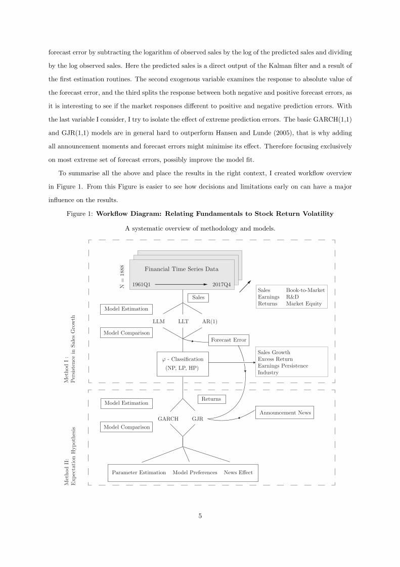
To summarise all the above and place the results in the right context, I created workflow overview

in Figure 1. From this Figure is easier to see how decisions and limitations early on can have a major

influence on the results.

Figure 1: Workflow Diagram: Relating Fundamentals to Stock Return Volatility

A systematic overview of methodology and models.

LLM LLT AR(1)

MethodI:

Persistence

inSales

Growth

MethodII:

ExpectationHypothesis

ϕ - Classification

GARCH GJR

1961Q1 2017Q4N = 1888

N=

1888 Financial Time Series Data

Sales Book-to-MarketEarnings R&DReturns Market Equity

(NP, LP, HP)

Model Estimation Model Comparison

Forecast Error Sales

Forecast Error Sales

Returns Announcement News

Returns Announcement News

Sales GrowthExcess ReturnEarnings PersistenceIndustry

Parameter Estimation Model Preferences News Effect

Model Estimation Model Comparison

Model Estimation Model Comparison

Model Estimation Model Comparison

5

The first block indicates financial time series data for around 1900 U.S. listed companies. These data

are drawn from both the CompuStat and the CRSP databases. The time series start in January 1961

until the end of December 2017, all companies need to report financial data for at least 25 years. This

strict limitation is enforced to end up with time series of at least around a hundred observations and so

support a solid time series analysis. The data consists of financial fundamental data such as performing

indicators, per-share variables, financial ratios and investment numbers seized on a quarterly frequency.

Data about the asset returns are sampled on a daily frequency and later transformed into weekly numbers

of returns and realised volatility. The data set is further extended with descriptive information about

industry, quarterly reporting dates and macro-economic variables such as the U.S. GDP numbers, the

returns of the S&P500 Index and the market volatility index, VIX.

The second block shows that from the optimal estimated model, I obtain a classification of the level

of persistence. A direct conclusion from the estimation routines is the rejection of the LLT model for

two third of the set of companies, fixing persistence at zero. By means of log-likelihood it proves hard

to justify the addition of two extra parameters. Based on this classification I form three portfolios, one

with non-persistent (NP), one low persistent (LP) and one high persistent (HP) companies. From these

portfolios I can conclude that the HP portfolio realises a sales growth than significantly outperform

the other two portfolios. This result remains unaffected by time span of the moving window and are

consistent over a the whole time period. As a whole I can conclude that for the HP portfolio sales are

predictable and high persistence results in high sales growth. The portfolio analysis does not show a

significant indication that high persistence is related to realising positive returns. But neither does it

point towards negative returns, as was found by Chan et al. (2003) and Chen (2017), who show that

portfolios of stocks with high sales growth realise a negative return. Although this is remarkable on its

own, it is important to mention that the returns are not corrected for the risk-free interest rate and

major market anomalies, such as size, value or momentum. There may be a strong relation between

sales and earnings, but after repeating the analysis with the earnings data, I show that there is minimal

correlation between both numbers of persistence and in line with Chan et al. (2003), earnings persistence

is even less frequent.

Continuing the workflow, I relate the persistence classification to GARCH volatility models. Firstly it

is important to review if stock returns are influenced by announcements. Throughout the literature, there

are multiple papers finding evidence of post-earnings-announcement drift, the tendency of returns to move

in the same direction as the earnings surprise. I altered the earnings surprise measure commonly used

in the literature, to the percentual forecast error from the Kalman filter. If I correlate the direction and

magnitude of this forecast error to the returns surrounding a week of announcement, I find a meagre, but

supporting indication that the proposed forecast error adds to explanation of variance. This indication

6

is further supported by the results of the model estimation routines, as for two third of the companies it

proves increase the fit. Out of this sub-sample, in one half of the cases only adding information about

announcement data provides an optimal fit. For the other half it is beneficial to include the forecast

error. It is important to highlight that this model preferences largely are indifferent for GARCH or GJR

models, indicating that the addition of a leverage term fails to dissolve the effects. To further check how

much the exogenous variables add to the explanation, I regress the estimated variance on the realised

variance with Mincer-Zarnowitz regression. By means of a percentual difference the R2 of log regression

is on average increased by around 7 %, taking only the companies into account where adding a variable

is preferred.

The portfolios formed earlier barely reveal differences among the three sub-groups: when I regard

model preferences it shows only minor differences. But with respect to the parameter estimates I conclude

that for the first, second and fourth estimated exogenous variables, their parameter distributions all

follow a similar pattern, and are not significantly different. However referring to the third variable,

which spliced between a positive and negative response, it shows that the HP portfolio shows a strong

effect. This implies that the stock market react stronger, leading to more volatility, when a firm from

the HP portfolio realises even better sales than were predicted. This finding is further confirmed by

significant difference in the news effect. Generally, it can be concluded that an announcement results in

a larger increase in volatility when the company is in the HP portfolio than in would in the NP portfolio.

Summarising over many companies and large time period may give vague intuition about how to

interpreted the results, therefore the last part focuses on a explicit case study between Apple and

Ford, that provides a more insightful figures and estimation results.

The remainder of this thesis is structured as follows: the next section gives an overview of the related

literature regarding the empirical relevance and motivation. The section after that reports the data, along

with summary statistics and relevant data transformations. Section 4 gives a broad introduction to the

theoretical background of state space modelling. Section 5 further discusses how state space modelling

is applied in this study, along with more methodological details, and it describes the configuration of

the volatility models. Section 6 presents the results, along with a detailed case study of two renowned

companies. Finally, Section 7 concludes this thesis by discussing suggestions for future research.

7

2 Literature Review

During the past decades, there has been an increasing amount of literature in the field of empirical and

quantitative finance regarding the universal questions ‘What strategies can predict stock prices?’, ‘Do

fundamentals give insight in stock price behaviour?’ and ‘Can we find the next ‘big thing’ in the stock

market?’. A large number of existing studies in a vast field of financial literature have examined these

questions, with limited success. In this study I will not claim to find the perfect solutions to the questions

stated above, but I aim to find a useful insight in the way financial markets operate. As the main point of

this research is to find the missing link between growth persistence in a companies fundamental numbers

and variation in stock returns, it covers a broad range of academic papers. To place this research in the

right context in the academic literature, the section below discusses the most relevant previous studies.

First, I will summarise the most recent views in the literature concerning the research. Next I will

describe the more general ideas about the empirical analysis of asset pricing and how this, and in particu-

larly fundamental sales data, relate to the market valuation of company. This will be followed by further

discussion about the persistence of cash flows and how state space modelling can capture this effect.

The fourth part will start with an explanation on how stock return volatility can by represented with

different types of GARCH models and will further elaborate on the connection between sales persistence

and return volatility. Finally, this section covers two market anomalies: an earning surprise that will lead

to unexpected returns or Post-Earnings-Announcement Drift and the Extrapolation Hypothesis, where

the latter was stated by La Porta (1996) as, the overreaction of investor to recent news.

I will start with recent evidence from a large empirical study of Chen (2017), who argues that contrary

of what might sounds reasonable, stocks with a low book-to-market ratio, popularised as growth stocks,

fail to pursue higher future cash flow growth rates. Stocks with high future growth rates have a longer

cash flow duration. This difference in duration could be seen as an important explanation for the value

premium of Fama and French (1992). The major results from Chen (2017) suggests that this difference

in duration alone as proposed in previous studies of Lettau and Wachter (2007, 2011) is implausible. The

duration explanation of the value premium rests upon two major elements, first the downward sloping

term structure of equity, assets with a long duration earn a lower return. And the second explanation

concludes that cash flows of growth stocks grow faster in comparison with value stocks. On both points

there is still a lot of debate going on in the literature. Regarding the first point it proves that only

for a small subset of models the term structure of equity is actually downward sloping, as reviewed in

Van Binsbergen et al. (2012). The second point, the relationship between a low book-to-market ratio and

a larger cash flow growth, has a lot of supporters as well as opponents. In 2004, Chen published a paper

which empirically finds support for this relationship, but e.g. Ang and Liu (2004) and several other

8

authors find opposing results, for example that dividends grow faster in value stocks. An overlooked

detail of his findings is that growth stocks have higher growth rates in sales and earnings in the first

year, but disappoint in the following years, which is in line with early work of Lakonishok et al. (1994).

One of the latest papers by Bordalo et al. (2017) extends the work of La Porta (1996), who showed

that companies with (over)optimistic long-term forecasts experience negative returns. In this recent

study they propose a theory of belief formation, which states that investors are forward looking in their

reaction to news items. Stated otherwise, they overreacted to information in the right direction. This

effect is captured in their model of formation diagnostic expectations and results in suitable explanations

for return anomalies and dynamics in fundamentals and returns.

The link between positive balance sheet fundamentals and negative future excess stock returns lately

has been reviewed in the work of Fisher et al. (2016). They reveal that systematic errors in investors’

long-term forecasts are reflected in stock prices and that these are consistent with return anomalies

generating mispricing. This bias in long-term growth forecasts relates back to research of La Porta

(1996), Dechow and Sloan (1997), Chan et al. (2003) and later Da and Warachka (2011), who find that

a strategy that focuses on short-term earnings forecasts is able to generate excess return.

The idea of this study is further motivated by a suggestion made in the paper of Lange and Teulings

(2018), where they openly question whether it is reasonable to assume that cash flows behave like a

random walk, which proves not the case, contrary to evidence found in early papers by e.g. Sloan (1996)

and Dechow et al. (1998).So, if there is predictability in cash flow growth, it also has some level of

persistence, but this persistence will not be permanent as it would otherwise suggest that cash flows of

current high-growth companies will be unbounded. For that reason it implies the use of a mean-reverting

model to capture these cash flow dynamics. This idea was also suggested in Fisher et al. (2016), as their

evidence is consistent with the view of professional analysts who believe that profits mean-revert, even

though profitability tends to have some level of persistence.

2.1 Empirical Stock Prices and Cash Flows

Relating back to literature of empirical stock pricing and following the timeline in financial economics

and financial mathematics, investors and other market participants always tried to find strategies that

provide accurate forecasts that are able to outperform the market. However, it was known from the

beginning of the nineteenth century that stock prices cannot be that easily predicted. The early work

of Fama (1965) on the behaviour stock market prices shows that they basically follow the random walk

principle and the following paper of Malkiel and Fama (1970) describes the Efficient Market Hypothesis,

which concludes that stock prices should reflect all publicly available information and every participant

9

interprets this information equally. It was this same Fama who in cooperation with French developed

a series of papers that showed that size (market equity) and value (book-to-market ratio) along with

market beta are important predictors for the cross-section of average stock returns (Fama and French

(1992, 1993)). In their 1995 paper they discuss how these factors can explain expectations in earnings.

Although these papers have proven their value, there is still a lot of debate in the literature about certain

assumptions underlying these models and about the possibility of other risk factors such as dividend rate,

low-volatility or industry. Lakonishok et al. (1994) claim that factors only represent systematic errors

in expectation about future returns, for example that excess return of high value stocks is a correction

for an irrational price and so that the stock market operates far from fully efficient. It states that

investors overprice growth stocks and underprice stocks that have performed poorly in the past, a view

widely shared in the field. Jegadeesh and Titman (1993) relate this to the momentum strategy, another

well-known market anomaly.

All these possible stock market strategies, essentially, intend to find one fundamental number: the

fair value of company. Numerous valuation methods are used in the literature, merely aiming to find the

present value of a companies future profitability. In the most general way, the fair value of a company is

defined as the expectation of the present value of the discounted future cash flows. Although this might

look relatively simple, it deals with two very complex highly uncertain components: future cash flows

and the rate at which this should be discounted. One of the early methods is the dividend discount

model, generally known as Gordon’s formula, which calculates the current stock price as the net value

of all future dividends. This would limit the valuation to only dividend-paying stock, therefore an

early adaption, initiated by Miller and Modigliani (1961), replaces dividends with earnings and uses the

growth in earnings in the denominator. Nowadays there are numerous papers relating market multiples

to company valuation and return e.g. dividend-price, earnings-price, earnings-per-share, sales-price, and

book value (Campbell and Shiller (1988), Ohlson and Juettner-Nauroth (2005) and many others). In

this research I use the time series properties to examine this specific effect in sales data. Although there

is a strong correlation between a companies fundamentals, the literature on the direct influence of sales

growth on the market valuation is limited. But depending on the valuation method, consistent sales

growth will have a positive effect on the markets view, trading it at higher multiples and possible lead

to negative returns, as was seen with other positive balance sheet fundamentals.

10

2.2 Persistence Sales Growth

An important work in the analysis of persistence in growth rates of companies comes from the paper of

Chan et al. (2003). Their work focuses on the question if it is likely that stocks preserve high growth

rates over multiple periods and if there is persistence in operating performance growth. They find that

long-term growth in earnings is not persistent, but sales to some extent are, and that numerous firms are

able to realise above median growth rates for successive years. As a possible explanation to this failing

persistence in earnings, Sloan (1996) and later Richardson et al. (2005) show that different earnings’

components have different levels of persistence and more specific that less reliable accruals lower this

persistence, while Dechow et al. (2008) find that persistence in the cash flow component solely relies

on a sub-component related to debt/equity dynamics. Later Kryzanowski and Mohsni (2014), show

that both components are mean-reverting and persistence weakens in a period with unfavourable growth

rates. Lacking persistence in earnings and accounting discrepancies causes this study merely to focus on

sales persistence.

Market participants always intend to find companies, ex ante, that will grow over the coming years,

but that remains very difficult. From a broad range of predicting variables, only expenses in R&D

and a company’s dividend policy prove to be of some worth. The work of Chan et al. (2001) highlight

that high intensive R&D companies tend to have more chances of future growth. While a company’s

dividend structure sends out important signals about attractive projects and possible future growth, low

current dividends results in high future growth per share. Further they underline that expectations of

growth rates should be able to reflect the cross-sectional variation in stock returns, but these market

expectations, proxied with analysts’ long-term forecasts, are mostly overly optimistic and these valuation

ratios fail to pick future winners or losers. These results are in line with the Extrapolation Hypothesis,

which states that current operating growth does not need to be extrapolated into possible future growth;

this is later confirmed by a large empirical study on US firms of Kryzanowski and Mohsni (2014).

The lack of major evidence that sales and other operating performers experience consecutive years of

growth might be caused by the idea that value companies are more settled in the market and exhibit little

volatility in returns or fundamentals, contrary growth stocks are highly volatile. First Lakonishok et al.

(1994) find that on a very short term extreme popular growth stocks experience higher growth rates,

but this dissolves over a longer time-span and they fall below the growth rates of value stocks. Later,

Chen (2017) concludes more generally that, contrary to what may be obvious, there is an insignificant

difference between the growth rates of future cash flows of growth stocks and value stocks.

There is a unambiguous relationship between stock price volatility and the volatility of accounting

fundamentals. Preliminary work on the high correlation between this relationship was undertaken by

11

Beaver et al. (1970), who concluded that market risk and risk in accounting measures are reflecting the

same underlying events and investors use this in their portfolio strategy. In the early days, the volatility

in stock prices ought to have a clear relation with a revision of expected future cash flows. A number of

authors recognised the shortcomings of this relation and that stock market volatility is not comparable

by for example the volatility of dividend rates (Shiller (1981)).

In the consecutive studies of Campbell and Shiller (1988), Campbell (1991), Campbell and Ammer

(1993) and Campbell and Kyle (1993), they find evidence that hints in the direction that stock prices are

way to volatile to be only caused by changes in expectation of future excess returns and the variance can

be decomposed into expectations about returns and cash flows. News about future cash flows explains

one third of the variance, the rest is due to news about unexpected future returns. Although there is

a high degree of correlation between both, an increase in the expectation of the future cash flows will

lead to a negative returns. Later research of Vuolteenaho (2002) contradicts these results, by claiming

that cash flow news is larger than expected return news on a firm level, because news about cash flows

is more company specific and can be largely diversified across a portfolio, while expected returns are

driven by macroeconomic components that affect the whole market. Callen and Segal (2004) mention

that information about accruals dominates expected return news and that changes in future accruals are

a primary driver of stock returns. The broader conclusion supported by Hecht and Vuolteenaho (2005)

and Sadka (2007) states that it is not possible to focus on the role of earnings on volatility without

taking stock returns into account due to the significant correlation between the two, but that stock price

volatility can to some extent be explained by the variation in expected earnings. Moreover, stock returns

are more altered by the changes in expectations rather than the actual level of earnings or returns.

2.3 Modelling Stock Return Volatility

Before further linking stock return volatility and the importance of a company’s fundamentals, I review

some groundbreaking papers that focus more specifically on the univariate modelling of asset price

volatility by Engle (1982) and Bollerslev (1986). In these papers the old-fashioned assumption of constant

volatility is dropped in favour of a (generalised) autoregressive conditional heteroskedastic volatility

process, GARCH, in which the current disturbances are sum of lagged previous squared observations

and/or disturbances. This approach rapidly became the industry’s workhorse in financial time series

analysis, as it is able to capture the stylised facts of asset pricing theory, such as volatility clustering

and leptokurtosis. This resulted in a legion of empirical studies as French et al. (1987), Campbell (1991)

amongst others, and model enhancements of which the GJR-model of Glosten et al. (1993) and EGARCH

of Nelson (1991) are the most renowned. The last two extensions make use of the fact that stock return

12

volatility has an asymmetric reaction to news, in which negative returns lead to a higher rise in volatility

levels than a positive return, further noticed as the leverage effect of news. A small set of studies extends

the model framework with exogenous variables, not in the last place as it proves hard to improve the

basic model (Hansen and Lunde (2005)). Sharma et al. (1996) find a significant variable in corresponding

trading volume, as a proxy for information arrival. The next to the leverage effect, the analysis of Glosten

et al. (1993) reports the significance for dummy variables for specific months. An important conclusion

of Andersen and Bollerslev (1998b) outlines the significant effect of U.S. macroeconomic announcement

moments to exchange rate volatility. Indicating the importance of announcement news, Blasco et al.

(2002) highlight that bad news is the main cause of asymmetric variance, and confirm the early findings

of Glosten et al. (1993)’s leverage effect. All these studies share the idea that GARCH models can

be improved, with model enhancements or extra variables. The relation with fundamentals has never

been fully investigated. With the macroeconomic announcement moments as a starting point, including

a companies own reporting announcements also might indicate a positive effect. From here one could

alter this announcement dummy with news about fundamentals, such as an adjustment in the amount

of realised earnings, a shift in dividend policy or change in investments strategy. A quarterly report

will always lead to different interpretations in the market. Most of the time these discrepancies dissolve

quickly and the market converges back to its temporary equilibrium. If the view of market participants

is not uniform, this will eventually create excessive volatility in the asset returns.

2.4 Extrapolation Hypothesis

The different perception of investors of news is exactly the line of thought that this thesis pursues to

find as a possible explanation to excessive volatility. The preliminary work was carried out several years

ago by De Bondt and Thaler (1985) with their paper on stock market overreaction, which concludes that

the market definitely overreacts in the direction of past out-performers and hence prior losers earn a

positive return compared to prior winners. This is later supported by the paper of La Porta (1996), who

uses financial analysts’ forecasts as a proxy to answer why the expected growth rates are systematically

inaccurate. He showed that these forecasts are too extreme in a sense that they assign multiples to

financial ratios that could almost never be realised, for gross of the companies. These high expectations

are believed to originate from the idea that investors overvalue recent news. He came up with the

Extrapolation Hypothesis, stated in his own words, “it takes time for investors to become aware of new

trends, but once they do, they often latch onto these perceived trend for too long”. Although he finds

warring results on a portfolio analysis on temporally winners and losers versus value and glamour stocks,

it could be concluded that glamour stocks are expected to be overpriced. What might sound reasonable

13

to some extent is that these glamour stocks carry way more risk. La Porta however provides evidence

that a risk based solution is not plausible and that high and low expected growth stocks are exposed

to the same levels of risk. Another striking result is that the expectations of predicted growth are very

often revised, providing evidence that analysts produce large forecasts errors in their level of earnings.

One might argue that if the growth of cash flows follows a more persistent pattern these revision are

less severe, because analysts have a better idea what to expect in the near future. In 1997, La Porta

et al. among others find that investors also overestimate the persistence in growth rates and extrapolate

these moments of realised growth; a result of Dechow and Sloan (1997) shows that earnings realise

only a half of what was expected by the analysts. This misinterpretation of non-existing persistence

leads to significant security mis-evaluation and controversy about security pricing undoubtedly results

in excessive volatility.

As a measure of excessive volatility I propose the following: if there would be no extrapolation

hypothesis in a sense that there is not any persistence in growth rates, every quarterly announcement

would be a relatively equal shock to the market and hence they would all be treated and evaluated

the same. But if there is at least some persistence in these growth rates, there might actually be a

decent guess of what the level of cash flows is going to be at the next announcement, and so the market

would exhibit lower excessive volatility. Two phenomena that relate to this are known throughout the

literature as earnings surprise and post-earnings-announcement drift (PEAD). Where the first describes

the difference between the reported earnings and the investors expectations, the latter describes the

upward movement of stock returns after a positive news announcement. It is reasonable to expect

that higher persistence in growth rates result into smaller variation between reported and expected

fundamental numbers. When a shock happens in these persistent growth rates, it will have a major

impact on investors, as it is hard to categorise this one-time shock as a short-term observation shock, a

mid-term level shock or a long-term trend shock. Although the interpretation of discrepancies varies, it

does result in an increase in volatility around such an announcement. If there is more consensus about the

direction of this surprise, many papers, among which Bernard and Thomas (1989), found evidence which

conclude a high correlation between this direction and the drift of cumulative returns. As many studies

provide different explanations for this abnormal returns I found one particular speculation of Daniel

et al. (1998) very notable, were they state that through the trigger of the earnings announcement the

overreaction in pre-event information produces the post-earnings-announcement drift. Further research

on PEAD is done by Ertimur et al. (2003) who propose that different market reactions to surprises

vary consistently between value and growth companies and on the level of sales persistence, and later

by Jegadeesh and Livnat (2006), who show that the magnitude in return drift depends heavily on the

magnitude of the sales surprise.

14

3 Data

From the CRSP / CompuStat Merged (North America) Fundamentals Annual Database I first obtain

the pre-sample data from all U.S. listed companies from 1950 until early 2018. Following the earlier

work of Da and Warachka (2009) and Chen (2017), I exclude companies not listed on one of the major

U.S. stock exchanges, other than NYSE, AMEX and NASDAQ, with corresponding exchange codes 11,

12 and 14 and Financial Services companies with SIC codes between 6000 and 6999. As for the sake of

this research only the companies which are reasonably long listed are included, I eliminate companies

which are delisted as a result of a merger or an acquisition, a default or a company going private. For

each company I need a complete data set from at least 25 years of sales data, which corresponds to at

least 100 quarterly observations. This restriction inevitable results in a very strong survivorship bias

within the data sample. After the elimination this concludes to a list of 1888 potential companies with 5

companies at the beginning of the sample, first quarter of 1961, but this inclines to 232 within a year and

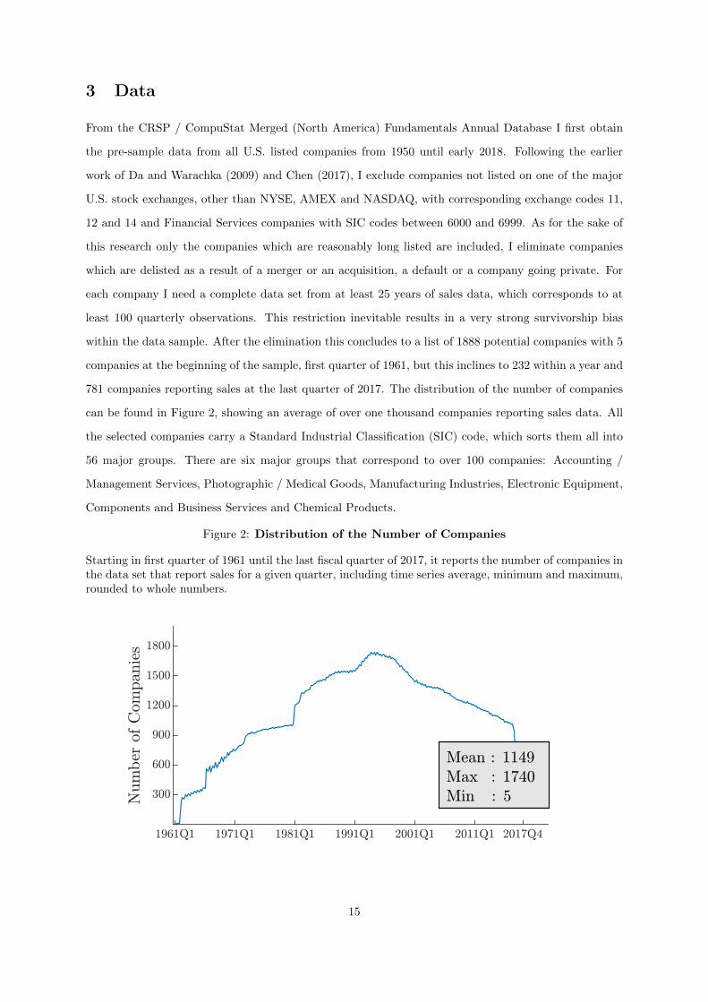
781 companies reporting sales at the last quarter of 2017. The distribution of the number of companies

can be found in Figure 2, showing an average of over one thousand companies reporting sales data. All

the selected companies carry a Standard Industrial Classification (SIC) code, which sorts them all into

56 major groups. There are six major groups that correspond to over 100 companies: Accounting /

Management Services, Photographic / Medical Goods, Manufacturing Industries, Electronic Equipment,

Components and Business Services and Chemical Products.

Figure 2: Distribution of the Number of Companies

Starting in first quarter of 1961 until the last fiscal quarter of 2017, it reports the number of companies inthe data set that report sales for a given quarter, including time series average, minimum and maximum,rounded to whole numbers.

15

This first indication of interesting companies is further examined in the Fundamentals Quarterly

Database. Not only will this increase the number of observation but it also allows for a detailed look

at specific time points. From this database I obtain the full data sample. This includes time series

per company on Market Equity, Book Equity, Sales, Earnings, R&D Expenses, Firm-Wide Investments,

Q-Ratio and two per share variables, Earnings- and Dividends per share. To elaborate more on the

details of the different variables, the section below gives an broader indication, the tickers represent the

CompuStat variables and their corresponding item number.

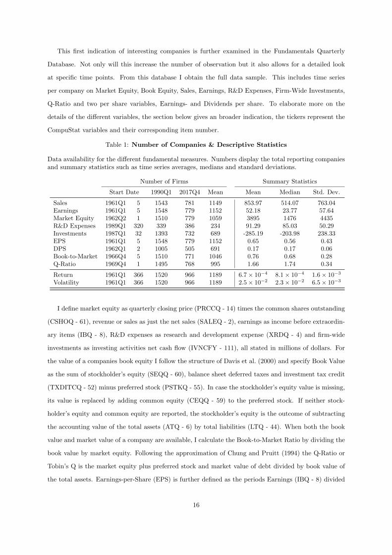
Table 1: Number of Companies & Descriptive Statistics

Data availability for the different fundamental measures. Numbers display the total reporting companiesand summary statistics such as time series averages, medians and standard deviations.

Number of Firms Summary Statistics

Start Date 1990Q1 2017Q4 Mean Mean Median Std. Dev.

Sales 1961Q1 5 1543 781 1149 853.97 514.07 763.04Earnings 1961Q1 5 1548 779 1152 52.18 23.77 57.64Market Equity 1962Q2 1 1510 779 1059 3895 1476 4435R&D Expenses 1989Q1 320 339 386 234 91.29 85.03 50.29Investments 1987Q1 32 1393 732 689 -285.19 -203.98 238.33EPS 1961Q1 5 1548 779 1152 0.65 0.56 0.43DPS 1962Q1 2 1005 505 691 0.17 0.17 0.06Book-to-Market 1966Q4 5 1510 771 1046 0.76 0.68 0.28Q-Ratio 1969Q4 1 1495 768 995 1.66 1.74 0.34

Return 1961Q1 366 1520 966 1189 6.7× 10−4 8.1× 10−4 1.6× 10−3

Volatility 1961Q1 366 1520 966 1189 2.5× 10−2 2.3× 10−2 6.5× 10−3

I define market equity as quarterly closing price (PRCCQ - 14) times the common shares outstanding

(CSHOQ - 61), revenue or sales as just the net sales (SALEQ - 2), earnings as income before extraordin-

ary items (IBQ - 8), R&D expenses as research and development expense (XRDQ - 4) and firm-wide

investments as investing activities net cash flow (IVNCFY - 111), all stated in millions of dollars. For

the value of a companies book equity I follow the structure of Davis et al. (2000) and specify Book Value

as the sum of stockholder’s equity (SEQQ - 60), balance sheet deferred taxes and investment tax credit

(TXDITCQ - 52) minus preferred stock (PSTKQ - 55). In case the stockholder’s equity value is missing,

its value is replaced by adding common equity (CEQQ - 59) to the preferred stock. If neither stock-

holder’s equity and common equity are reported, the stockholder’s equity is the outcome of subtracting

the accounting value of the total assets (ATQ - 6) by total liabilities (LTQ - 44). When both the book

value and market value of a company are available, I calculate the Book-to-Market Ratio by dividing the

book value by market equity. Following the approximation of Chung and Pruitt (1994) the Q-Ratio or

Tobin’s Q is the market equity plus preferred stock and market value of debt divided by book value of

the total assets. Earnings-per-Share (EPS) is further defined as the periods Earnings (IBQ - 8) divided

16

by the shares outstanding and the same holds for the Dividends-per-Share (DPS), where I use dividends

preferred (DVPQ - 24) respectively or if either the preferred dividends or common shares outstanding is

missing I obtain the DPS value directly from CompuStat (DVPSPQ - 16).

Although the data set is not excessively large, there are still quite some missing observations, which

depends on a lot of factors. Table 1 reports the first observation of the different variables, which indicates

that from 1989Q1 all the variables are reported and at the beginning of the sample, 1961Q1 - 1971Q1

there is limited availability for most of the variables. Another issue that arises is that not every company

pays out dividends or fully reports its quarterly investments. What often occurs is a full series of quarterly

observations and occasionally a run of three missing observations and a cumulative sum at the fourth

index. It makes sense that this last cumulative observation will have a large impact. Therefore I divide

this ‘annual’ number by four to obtain a reasonable ‘quarterly’ number.

To extend the data set with stock return and volatility data, I link the selected companies to a

unique CRSP code. From the Daily Stock File I extract stock prices, number of shares outstanding and

(delisting) returns from January first 1961 until December 31st 2017. Quarterly (weekly) returns and

volatility are calculated as respectively the mean and standard deviation of daily stock returns within a

quarter (week) and, if necessary, using the delisting return as last possible observation.

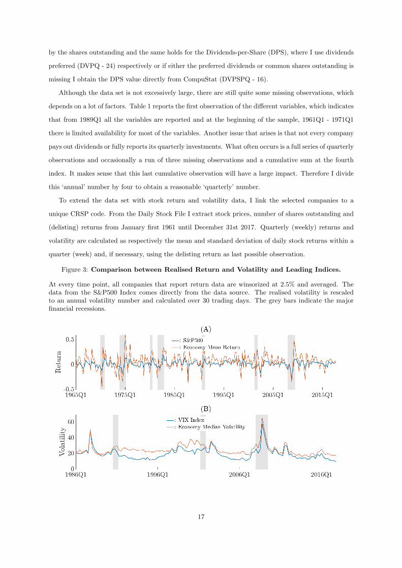
Figure 3: Comparison between Realised Return and Volatility and Leading Indices.

At every time point, all companies that report return data are winsorized at 2.5% and averaged. Thedata from the S&P500 Index comes directly from the data source. The realised volatility is rescaledto an annual volatility number and calculated over 30 trading days. The grey bars indicate the majorfinancial recessions.

17

As a validity check I compared the average of the quarterly returns of the companies with the

return of the S&P500 Index. At every point in time I exclude returns above the 97.5th and below the

2.5th percentile and calculate the mean over all companies, to minimise the effect of the most extreme

observations. Figure 3A shows that the returns tend to follow the pattern of the S&P500 Index, but

has more extreme returns, due to the strong presence of the survivorship bias. Likewise I compare the

volatility of the stock returns with the CBOE Volatility Index or VIX. First, I rescale the quarterly

volatility to an annual volatility number and by definition of the VIX, annualised implied volatility over

30 trading days, multiply the annual volatility by the square-root of 30. In the same way as it does with

the return data, the mean of the stock return volatility clearly follows the same pattern (Figure 3B),

but is often too extreme.

18

4 State Space Modelling

To look deeper in the empirical part of this research, I use data which follows various companies with

multiple financially descriptive variables over a large time period. The choice to analyse individual firms

as univariate time series opens the world to state space modelling, this section gives a brief theoretical

background, and is preliminary to methodology used later in this study. As further described below, this

method is particularly useful when data is prone to observational noise and seasonal effects. Additionally,

it has the possibility to capture growth in a more smoothed way in one of the latent states. Using state

space modeling on sales data to capture a firms sales growth has not yet been seen in literature. This

is particularly remarkable because in 1974, Lev and Kunitzky showed that sales systematically follow

growth trends over time and therefore are favourable to smoothing algorithms. But this absence of later

studies is probably due to limited available data: time series analyses lose parameter significance when

there are a low number of observations. To partially overcome this issue, I limit the study to companies

that have at least 25 years of sales data, between 1961 until December 2017. A downside of this solution

is the inevitable survivorship and backfill biases, which should be addressed appropriately. This mainly

implies that the reported growth rates should be interpreted with care. To provide further details on

state space modeling, the section below strats with the general state space setup, after which it explains

the Kalman filtering technique and ends with an estimation routine.

4.1 General State Space Model

Starting with the most general form of a state space model, I choose to follow the notation of Durbin

and Koopman (2012) and Harvey (1990). In a General Linear Gaussian State Space Model a time series

starting at t = 1 until t = T can be described by its observation and state equations:

yt = Z ′tαt +Ωtdt + εt, εt ∼ N(0,Ht),

αt+1 = Ttαt +Φtct +Rtηt, ηt ∼ N(0,Qt), t = 1, ..., T .(1)

The observation equation consist of the observation vector yt, which is a q× 1 column vector, where q is

the number of observed dependent variables, k exogenous variables through a k×1 vector dt, along with

q×k matrix Ωt and observations noise via εt which has the same dimension as yt. The state vector αt is

a m×1 vector with m unobserved latent states, which access the observation vector through a q×m row

vector Z ′t. In the state equation, the states have a dependence due to the m×m transition matrix Tt. It

further contains a s×s matrix of s exogenous variables ct multiplied by m×s matrix Φt and a disturbance

term in which the m×g matrix Rt and g×1 vector ηt adds noise to the states. The observation variance

matrix Ht and the state variance matrix Qt are assumed to be independent and serially uncorrelated,

19

and in case of the Gaussian model, normally distributed. Where the first and second assumption are a

key requirement to rightfully identify the model, the last assumption could be dropped and the model

in Equation 1 generalises to the General Linear State Space Model. The matrices Z ′t,Tt,Rt,Ht,Qt,Φt

and Ωt are the system matrices of the state space model and are generally unknown and result from an

estimation routine, further described in the next section. The initial state α1 is a draw from N(a1,P1),

independent of the observation and state disturbances and with a1 and P1 assumed to be known or

diffuse. The subscript t in the system matrices allows them to be time-variant, but for the sake of the

scope of this project, the subscript will be dropped at all system matrices, making them constant over

time.

4.2 Univariate Time Series Models

The two basic cases of the general state space model are the local level model (LLM) and the local linear

trend model (LLT). In the univariate case without exogenous variables, where we observe only a single

time series yt, the LLM has only a single latent state, the level state µt, by means of Equation 1:

Z ′ = 1, H = σ2ε , Ω = 0, dt = 0, Q = σ2

η, Φ = 0, ct = 0, αt = µt, T = 1, R = 1,

resulting in:

yt = µt + εt, εt ∼ N(0, σ2ε),

µt+1 = µt + ηt, ηt ∼ N(0, σ2η), t = 1, ..., T .

(2)

In this model, µt follows a random walk plus drift, as all random variables are normally distributed,

all εt’s and ηt’s are uncorrelated, serially independent and constant over time. The local level model as

described in Equation 2 contains two unknown parameters, σ2ε and σ2

η, which need to be estimated from

the observed data. It possible to alter the basic LLM to a LLT model with the addition of a stochastic

slope term δt in the unobserved level equation.

yt = µt + εt, εt ∼ N(0, σ2ε),

µt+1 = µt + δt + ηt, ηt ∼ N(0, σ2η),

δt+1 = δt + ζt, ζt ∼ N(0, σ2ζ ), t = 1, ..., T .

(3)

The extension of the stochastic slope leaves the model with three instead of two unknown parameters,

σ2ε , σ2

η and σ2ζ . To express this LLT model in the way of the general state space model of Equation 1,

20

the system matrices become:

Z ′ =

(1 0

), H = σ2

ε , αt =

µt

δt

, T =

1 1

0 1

, Q =

σ2η 0

0 σ2ζ

, R =

1 0

0 1

,

and further there are no exogenous variables, so dt = 0, Ω = 0, ct = 0, and Φ = 0.

4.3 Kalman Filter and Smoother

From the general state space model in Equation 1, it is generally known that the state space vector is not

observed, which limits the ability to directly distinguish important signals from arbitrary short-lasting

noise. This contamination of signal and noise is overcome by the use of the Kalman Filter (Kalman, 1960;

Kalman and Bucy, 1961). This set of recursive formulas leads to a algorithmic procedure to compute

the optimal estimator of the state vector at time point t, using only the available information upon this

time point, updating the estimator every time a new observation comes in. The purpose of the filter is

to obtain a conditional distribution of αt and αt+1 given the information at time t, It. The Kalman

filter starts with the best possible prediction of the next state via the prediction equations,

αt+1|t = T αt|t +Φct,

Pt+1|t = TPt|tT′ +RQR′, t = 1, ..., T ,

(4)

and when a new observation yt comes in, updates its best prediction via the updating equations,

αt+1|t+1 = αt+1|t + Pt+1|tZ(Z ′Pt+1|tZ +H)−1(yt −Z ′αt|t −Ωdt)

Pt+1|t+1 = Pt+1|t − Pt+1|tZ(Z ′Pt+1|tZ +H)−1Z ′Pt+1|t, t = 1, ..., T .(5)

This set of equations starts with the initial values for the best prediction of α1|0 and covariance matrix

of the prediction error P1|0 and iterates forward through the data sample. In many cases I use diffuse

initialisation, as there is minimal information about the initial state, which implies that initial state

is equal to its unconditional mean and the initial covariance is set to the unconditional covariance,

α1|0 ∼ N(0, κI), where κ → ∞. If there is some information about (part of) the initial state, the

variance could be reduced or at least shrunk to the same order of magnitude as information about the

state. At the end of the sample T , we have information on the complete data set and are able to provide

21

even better estimates of the states. This is done by the Kalman (fixed-interval) smoothing equations,

αt|T = αt|t + Pt|tT′P−1t+1|t(αt+1|T − αt+1|t)

Pt|T = Pt|t − Pt|tTP−1t+1|t(Pt+1|t − Pt+1|T )P−1t+1|tTPt|t.(6)

The smoother starts at the end of the data sample and iterates backward to initial values. The option

to use both the filter and the smoother provides more accurate state estimates, as can be seen from the

second term in Equation 6, which will decrease the current state covariance. The complete derivation of

the recursive formulas of the Kalman filter and smoother can be found in Appendix A.1.

4.4 Parameter Estimation

The system matrices, used by the Kalman filter and smoother contain several unknown parameters,

which need to be estimated from the data. The estimation of the parameters is done by maximising the

Likelihood function and the Expectation Maximisation algorithm.

The theory of Maximum Likelihood (ML) uses the assumption that observation are all independent

of each other and the likelihood function or joint probability density function (p.d.f.) of the sample is

the product of the individual p.d.f.’s. The function needs to be optimised to obtain the ML estimator.

In the case of the state space model, observations are not independent due to dynamics in the state

equation via transition matrix T and hence it is not applicable to use this likelihood function. To obtain

a valid ML estimator, the joint p.d.f. can be rewritten as the product of the conditional p.d.f.’s

L(y1, ..., yT ;θ) = p(y1, ..., yT ;θ) =

T∏

t=1

p(yt|It−1, ..., I1;θ), (7)

where p(yt) is the p.d.f. of the t-Th observation, It is all the information available upon time t and θ is

parameter vector that maximises the likelihood function. When intensively using the normal distribution,

the log-likelihood function `(yt;θ) is often preferred instead of the likelihood function in Equation 7,

because the sum-product turns into a simple summation,

`(y1, ..., yT ;θ) = log(L(y1, ..., yT ;θ)) =

T∑

t=1

log(p(yt|It−1;θ))

= −T2

log(2π)− 1

2

T∑

t=1

log(|Σt(θ)|)− 1

2

T∑

t=1

(yt − µt(θ))′(Σt(θ))−1(yt − µt(θ)).

(8)

The application of this concept in the framework of state space models is best described by (Harvey,

1990) and is known as prediction error decomposition. Based on the assumption that all disturbance

terms in model Equation 1 are normally distributed and the lemmas associated with handling normal

22

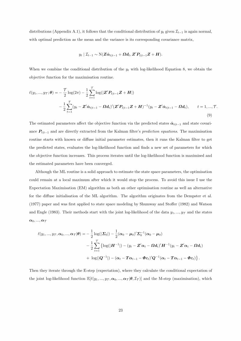
distributions (Appendix A.1), it follows that the conditional distribution of yt given It−1 is again normal,

with optimal prediction as the mean and the variance is its corresponding covariance matrix,

yt | It−1 ∼ N(Zαt|t−1 +Ωdt,Z′Pt|t−1Z +H).

When we combine the conditional distribution of the yt with log-likelihood Equation 8, we obtain the

objective function for the maximisation routine.

`(y1, ..., yT ;θ) =− T2

log(2π)− 1

2

T∑

t=1

log(|Z ′Pt|t−1Z +H|)

− 1

2

T∑

t=1

(yt −Z ′αt|t−1 −Ωdt)′(Z ′Pt|t−1Z +H)−1(yt −Z ′αt|t−1 −Ωdt), t = 1, ..., T .

(9)

The estimated parameters affect the objective function via the predicted states αt|t−1 and state covari-

ance Pt|t−1 and are directly extracted from the Kalman filter’s prediction equations. The maximisation

routine starts with known or diffuse initial parameter estimates, then it runs the Kalman filter to get

the predicted states, evaluates the log-likelihood function and finds a new set of parameters for which

the objective function increases. This process iterates until the log-likelihood function is maximised and

the estimated parameters have been converged.

Although the ML routine is a solid approach to estimate the state space parameters, the optimisation

could remain at a local maximum after which it would stop the process. To avoid this issue I use the

Expectation Maximisation (EM) algorithm as both an other optimisation routine as well an alternative

for the diffuse initialisation of the ML algorithm. The algorithm originates from the Dempster et al.

(1977) paper and was first applied to state space modeling by Shumway and Stoffer (1982) and Watson

and Engle (1983). Their methods start with the joint log-likelihood of the data y1, ..., yT and the states

α0, ...,αT

`(y1, ..., yT ,α0, ...,αT |θ) =− 1

2log(|Σ0|)−

1

2(α0 − µ0)′Σ−10 (α0 − µ0)

− 1

2

T∑

t=1

log(|H−1|)− (yt −Z ′αt −Ωdt)′H−1(yt −Z ′αt −Ωdt)

+ log(|Q−1|)− (αt − Tαt−1 −Φct)′Q−1(αt − Tαt−1 −Φct).

Then they iterate through the E-step (expectation), where they calculate the conditional expectation of

the joint log-likelihood function E[`(y1, ..., yT ,α0, ...,αT |θ, IT )] and the M-step (maximisation), which

23

maximises the conditional expectation over the parameters,

∂

∂θE[`(y1, ..., yT ,α0, ...,αT |θ, IT )] = 0. (10)

The derivation of Equation 10 for all the system matrices and vectors of a general state space model is

further elaborated in Appendix A.2. The resulting set equations lets the estimated parameters converge

relatively quickly into a local maximum and does not depend heavily on the initial starting values.

This proves useful as starting values lead to another problem in the parameter estimation procedure,

the initialisation of the state space model. The estimation routine depends on the initial parameter

values and has major influences on the convergence of the parameters. Before starting the parameter

estimation and the Kalman filter, it proves difficult to find a solid set of initial parameter estimates, e.g.

Kitagawa and Gersch (1984) and De Jong (1991). I choose to derive some indication of initial values

from the variance and auto-correlation structure of the first differences of the observations. The full

derivation is found in Appendix A.3. But results for a univariate local level model, as long as both σ2ε

and σ2η are in the same order, it is useful to set the initialisation approximately to

σ2ε =

1

4Var(yt − yt−1), σ2

η =1

2Var(yt − yt−1).

The same goes for a local linear trend model, if again σ2ε , σ2

η and σ2ζ are of equal magnitude a proper

starting value is

σ2ε =

1

6Var(yt − yt−1), σ2

η =1

3Var(yt − yt−1), σ2

ζ = (1− ϕ2)1

3Var(yt − yt−1).

Here I use the exponent of the coefficient from the OLS regression of log autocovariance of the first

differences on lag-order multiplied by the log of ϕ as an starting value for ϕ.

24

5 Methodology

In this chapter I will explain the two main methods used in this study. The first section focuses on

the estimation procedure of the state-space model and how this can be implemented to estimate the

persistence of sales growth in a mean-reverting local linear trend model. In the second section I use

the estimated sales growth to describe how the extrapolation hypothesis leads to a misvaluation in the

market and hence, leads to excessive volatility in stock returns.

5.1 Persistence in sales growth

It is widely accepted that sales and through some extent also sales growth show some level of predict-

ability. The chances that high potential glamour stocks as Alphabet.Inc and Amazon.com will have

expanding revenues in the coming years are much more likely than that large value stock will show

recurrent sales growth. In the literature this persistence in (sales) growth is usually captured by the runs

of successive years or months of growth and as a result the papers of Chan et al. (2003) and Chen (2017)

show a very limited amount of companies that is able to achieve this continuing growth. To step away

from this ‘successive-run’ approach I choose a different, yet unexplored approach to measure the sales

growth persistence of U.S. companies. At the bottom of this new approach lies the favourable tendency

to model time series data by means of a General State Space Model. This model allows to decompose the

noisy and seasonally affected sales data into smooth level, trend and seasonal components. The trend

component can be interpreted as the sales growth and hence we can extract some measure of persistence

from this estimated trend. To give a more economic interpretation at this measure of persistence, I

relate the estimated trend component to the average growth of sales in the data sample, which can be

seen as the average sales growth of the economy. If a company is able to realise consecutive periods

of out (under)performance of the economy’s average sales growth, this can be seen as a strong growth

persistence. However, it proves difficult for many companies to achieve such market out-performance,

and hence most of the time a company’s sales growth is fluctuating around the market average. Sales

growth can be seen as a mean-reverting autoregressive process, with a economy average as a time varying

mean and a persistence parameter corresponding with the speed of mean-reversion.

Therefore I consider three different models to find this persistence parameter. Two of them are using

the state space approach on the sales observations and the third approach focuses directly on finding a

autoregressive relation in realised sales growth. The second state space model is a wider extension of the

first, or the first model restricts some model parameters. The third autoregressive model is also nested

in the second state space model. A systematic overview can be found in Figure 4.

The first state space model is an extension of the basic local level model. I include seasonal components

25

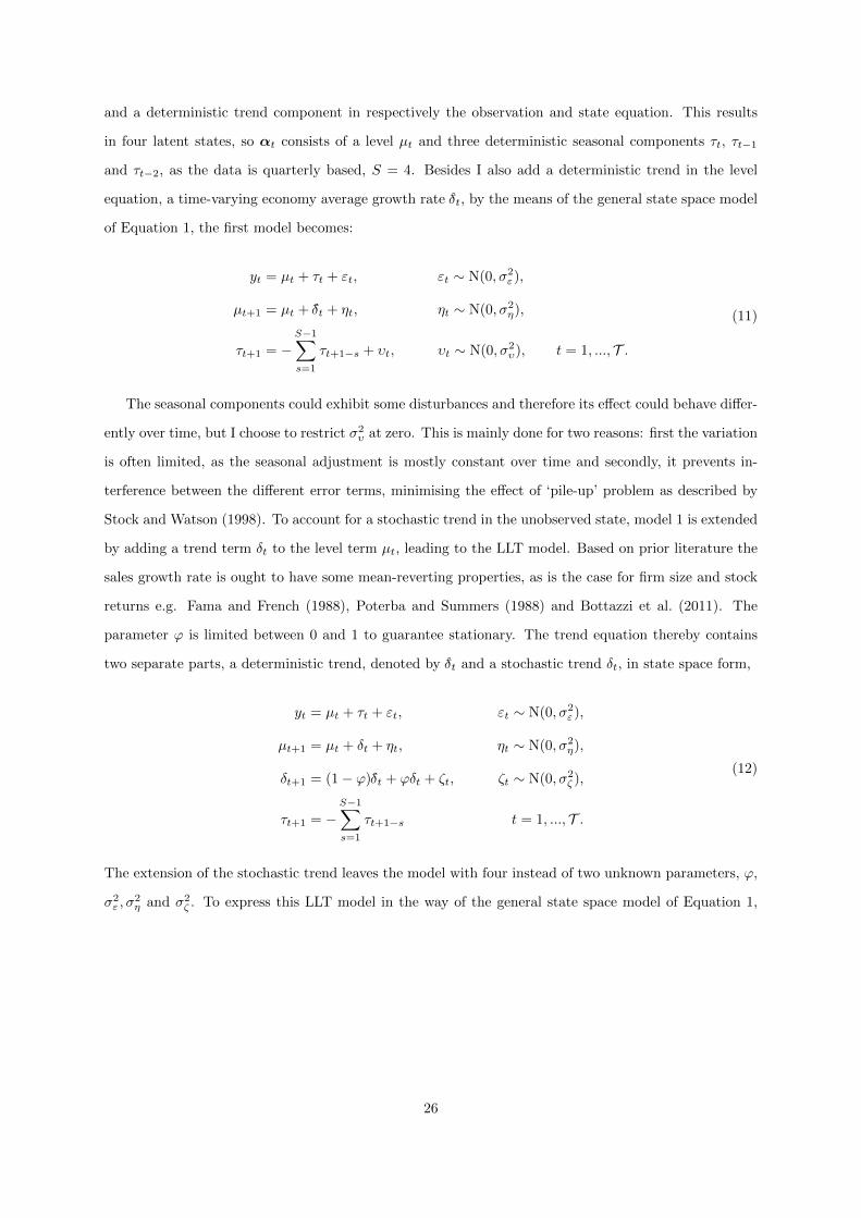
and a deterministic trend component in respectively the observation and state equation. This results

in four latent states, so αt consists of a level µt and three deterministic seasonal components τt, τt−1

and τt−2, as the data is quarterly based, S = 4. Besides I also add a deterministic trend in the level

equation, a time-varying economy average growth rate δt, by the means of the general state space model

of Equation 1, the first model becomes:

yt = µt + τt + εt, εt ∼ N(0, σ2ε),

µt+1 = µt + δt + ηt, ηt ∼ N(0, σ2η),

τt+1 = −S−1∑

s=1

τt+1−s + υt, υt ∼ N(0, σ2υ), t = 1, ..., T .

(11)

The seasonal components could exhibit some disturbances and therefore its effect could behave differ-

ently over time, but I choose to restrict σ2υ at zero. This is mainly done for two reasons: first the variation

is often limited, as the seasonal adjustment is mostly constant over time and secondly, it prevents in-

terference between the different error terms, minimising the effect of ‘pile-up’ problem as described by

Stock and Watson (1998). To account for a stochastic trend in the unobserved state, model 1 is extended

by adding a trend term δt to the level term µt, leading to the LLT model. Based on prior literature the

sales growth rate is ought to have some mean-reverting properties, as is the case for firm size and stock

returns e.g. Fama and French (1988), Poterba and Summers (1988) and Bottazzi et al. (2011). The

parameter ϕ is limited between 0 and 1 to guarantee stationary. The trend equation thereby contains

two separate parts, a deterministic trend, denoted by δt and a stochastic trend δt, in state space form,

yt = µt + τt + εt, εt ∼ N(0, σ2ε),

µt+1 = µt + δt + ηt, ηt ∼ N(0, σ2η),

δt+1 = (1− ϕ)δt + ϕδt + ζt, ζt ∼ N(0, σ2ζ ),

τt+1 = −S−1∑

s=1

τt+1−s t = 1, ..., T .

(12)

The extension of the stochastic trend leaves the model with four instead of two unknown parameters, ϕ,

σ2ε , σ

2η and σ2

ζ . To express this LLT model in the way of the general state space model of Equation 1,

26

the system matrices and vectors become:

Z ′ =

(1 0 1 0 0

), H = σ2

ε , ,dt = 0 Ω = 0, Q =

σ2η 0

0 σ2ζ

, ct = δt,

T =

1 1 0 0 0

0 ϕ 0 0 0

0 0 −1 −1 −1

0 0 1 0 0

0 0 0 1 0

, αt =

µt

δt

τ1,t

τ2,t−1

τ3,t−2

, R =

1 0

0 1

0 0

0 0

0 0

, Φ =

0

(1− ϕ)

0

0

0

.

The LLT model as described above suggests two limiting cases,

1. If the trend is utterly persistent and ϕ → 1, the growth is completely stochastic and follows a

random walk with variance σ2ζ . In this case, there is no mean-reversion and model 2 acts as a basic

local linear trend model.

2. If the mean-reversion parameter ϕ = 0, the dependence structure on the previous growth is altered

and becomes δt = δt + ζt and the state equation converts to µt = µt−1 + δt + ηt + ζt. In this

particular situation, both the error terms σ2η and σ2

ζ are not separately identified and the model

produces uninterpretable estimates, unless we restrict σ2ζ to zero. If both ϕ = 0 and σ2

ζ = 0 the

local linear trend model is exactly the same as the local level model with the deterministic trend

in model I.

In the third approach to find a persistence parameter ϕ, I directly apply an auto-regressive model of

the first order AR(1) on the growth in sales, ∆yt = yt − yt−1, resulting in model 3:

∆yt = ϕ∆yt−1 + ζt, ζt ∼ N(0, σ2ζ )

(yt − yt−1 − δt) = ϕ (yt−1 − yt−2 − δt−1) + ζt, t = 3, ..., T .(13)

It proves an easy exercise to convert this AR(1) model into a state space form:

Z ′ = 1, H = 0, dt = 0, Ω = 0, Q = σ2ζ , ct = 0, Φ = 0, αt = ∆yt−1, T = ϕ, R = 1.

To estimate the unknown parameters for the three different models, I start with finding reasonable

initial starting values for the optimisation routine, as further described in Section 4. For the first two

models, the step-by-step approach is listed below. After the determination of good initial starting values,

I estimate a simplistic local level model without any trend to update the initial values and optimise model

I. Likewise I use the estimates from model I to update the initial values for model II. This proves useful as

27

it speeds up the calculation, but on the other hand could restrain the optimisation in a local minimum.

Therefore every model is estimated twice with maximum likelihood, with updated initials and with

diffuse initialisation and also once with the EM algorithm. With the EM algorithm I iterate 500 times, a

number at which most parameters have converged1. Although the parameters mostly converged, the EM

algorithms turns out to be of limited success, because the model implies certain parametric restrictions,

which do not come trivial within the EM algorithm. To summarise the estimation routine for the two

state space models, the four steps below are repeated for every company:

Step 1: Find initial starting values based on the autocorrelation structure and variance of the first differ-

ences.

Step 2: Model 0 : Estimate a Local Level Model with δt = 0, implying that the trend is zero.

Step 3: Estimate model I : use model 0 as updated initialisation.

Step 4: Estimate model II : us model I as updated initialisation.

The estimation routine for the AR(1) model, differs a bit from the above in a sense that I use two

different approaches, in the first I use a regression estimate and the second approach uses the state space

setup.

1. Regression Approach: to find the OLS estimate for the persistence, I regress ∆yt on ∆yt−1 and

residuals lead to an estimate for the variance.

2. State Space Approach: rewrite the AR(1) model in state space form and evaluate the likelihood

function as with the other two models.

Both approaches rest upon the same set of assumptions, but in the regression approach it comes unnatural

to restrict model coefficients; therefore it is often not applicable for the purpose of this research.

After all the optimisation routines, it results in a total of 8 sets of estimated parameters per company,

three models with two or three routines. First I select is best set of parameters within each model based

on the highest likelihood and if all parameter restrictions are met. This is equal to a selection based on

Akaike Information Criteria, where there is no difference in the number of parameters. In the ideal case,

all likelihoods are generally the same, and the difference is purely a numerical issue.

Next I choose the model that fits best to the data. Figure 4 shows how this is done. Due to the

fact that model I is nested in model II, a Likelihood Ratio test provides a good way to select the best

model based on goodness of fit on the data. The same accounts for selecting model III or model I. In

1Sample-wise I have increased the number of iterations above 500 to increase the algorithms performance, but theseresults were limited and unnecessary increased the computational burden.

28

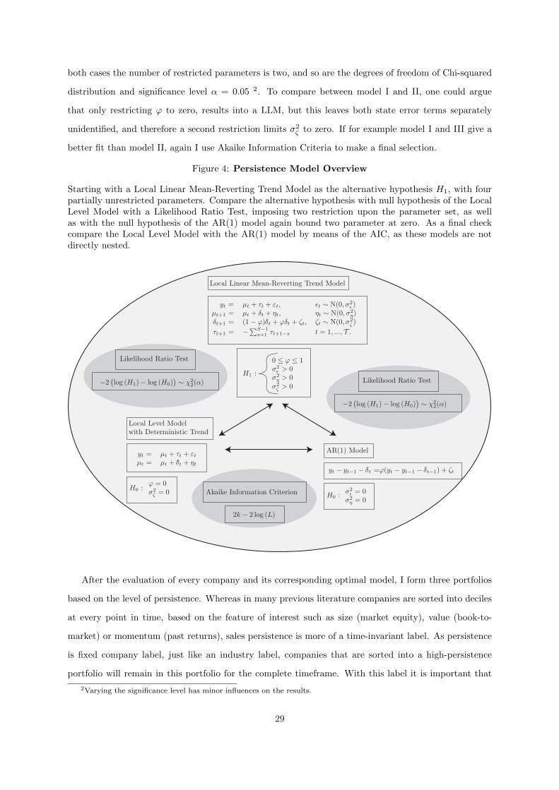
both cases the number of restricted parameters is two, and so are the degrees of freedom of Chi-squared

distribution and significance level α = 0.05 2. To compare between model I and II, one could argue

that only restricting ϕ to zero, results into a LLM, but this leaves both state error terms separately

unidentified, and therefore a second restriction limits σ2ζ to zero. If for example model I and III give a

better fit than model II, again I use Akaike Information Criteria to make a final selection.

Figure 4: Persistence Model Overview

Starting with a Local Linear Mean-Reverting Trend Model as the alternative hypothesis H1, with fourpartially unrestricted parameters. Compare the alternative hypothesis with null hypothesis of the LocalLevel Model with a Likelihood Ratio Test, imposing two restriction upon the parameter set, as wellas with the null hypothesis of the AR(1) model again bound two parameter at zero. As a final checkcompare the Local Level Model with the AR(1) model by means of the AIC, as these models are notdirectly nested.

yt = µt + τt + εt, ǫt ∼ N(0, σ2ǫ )

µt+1 = µt + δt + ηt, ηt ∼ N(0, σ2η)

δt+1 = (1− ϕ)δt + ϕδt + ζt, ζt ∼ N(0, σ2ζ )

τt+1 = −∑S−1s=1 τt+1−s t = 1, ..., T .

Local Linear Mean-Reverting Trend Model

H1 : 0

: 0 ≤ ϕ ≤ 1σ2ǫ > 0

σ2η > 0

σ2ζ > 0

yt − yt−1 − δt =ϕ(yt − yt−1 − δt−1) + ζt

AR(1) Model

σ2ǫ = 0

σ2η = 0

H0 :

yt = µt + τt + εtµt = µt + δt + ηt

Local Level Modelwith Deterministic Trend

y = µ + τ + ε

H0 :ϕ = 0σ2ζ = 0

−2(log (H1)− log (H0)

)∼ χ2

2(α)

Likelihood Ratio Test

( )

Akaike Information Criterion

2k − 2 log (L)

−2(log (H1)− log (H0)

)∼ χ2

2(α)

Likelihood Ratio Test

( )

After the evaluation of every company and its corresponding optimal model, I form three portfolios

based on the level of persistence. Whereas in many previous literature companies are sorted into deciles

at every point in time, based on the feature of interest such as size (market equity), value (book-to-

market) or momentum (past returns), sales persistence is more of a time-invariant label. As persistence

is fixed company label, just like an industry label, companies that are sorted into a high-persistence

portfolio will remain in this portfolio for the complete timeframe. With this label it is important that

2Varying the significance level has minor influences on the results.

29

the portfolios are not too meagre, otherwise it could be that only a small number of companies represent

a whole portfolio at a certain time point, which would make it very susceptible to possible extreme

observations. To examine most of the insightful portfolio features, the portfolios are later double sorted

according to the weighted average rank of sales growth (WGS), so every portfolio is spilt again into

three sub-portfolios. For example, for the annualised one year sales growth, every company within the

portfolio that has reported sales over the previous year is ranked at every time point t. This rank is

weighted and averaged over the last 2 years, or 8 quarterly observations, according to a weight of 8/36

for t − 1, 7/36 for t − 2 and so on, to reduce the possible seasonal effects and aberrant observations.

Based on this weighed average rank, the sub-portfolios are constructed according to a 30/40/30 percent

principle and a restriction of a least a numerous amount of reporting companies at the specific time point

and portfolio.

5.2 Extrapolation Hypothesis

The major goal of the research is to link the persistence of and predicted sales growth to possible stock

misvalution. As finding the ‘true’ value of stock is providing work for a whole industry, a good proxy for

this matter is to look at role of post-earnings-announcement drift (PEAD) in stock return volatility. If

the whole market is sure about a company’s future expectation, return and hence stock volatility remain

close to the conditional average. But if there is any inconsistency in the market about how to react to

the newly announced report, this will lead to discrepancy in the stock return and consequently to higher

volatility. In short, post-earnings-announcement drift leads to a drift in the cumulative stock returns in

the direction of the earnings surprise. To link this to differences in sales persistence, one would expect

that for companies with a higher sales persistence, the market is more consistent about the upcoming

report and so will have a lower earnings surprise and is less affected by post-earnings-announcement

drift.

To model the volatility of stock returns I use the popular generalised autoregressive conditional

heteroskedasticity framework from Bollerslev (1986). This class of models is able to explain most of the

stylised facts of empirical asset returns, non-normal distribution and no correlation in the returns and

strong correlation in the absolute returns. In the most general setup for a model to capture volatility

clustering, the weekly return rt is represented by a GARCH(1,1) model,

rt = ψ + νt

νt = zt√ht, zt ∼ N(0, 1)

ht = ω + λ1 ν2t−1 + β1 ht−1 t = 1, ..., T ,

(14)

30

with an unconditional mean ψ, a standard random walk process νt and a time-varying conditional

variance ht, with the restriction that ω > 0, λ1 ≥ 0, β1 ≥ 0, so that the volatility will be positive for

every t and λ1 + β1 < 1 to ensure the model is covariance stationary.

A common extension of the ‘simple’ GARCH(1,1) model is the introduction of asymmetric GARCH

models. In this research I use a Threshold GARCH model from Glosten et al. (1993), further noted

as the GJR model. The main idea behind asymmetric models is that positive and negative returns

have different effect on the volatility, and it is basically known that (large) negative returns lead to an

increased volatility, also known as the leverage effect. For the GJR model, the ht equation from the

standard GARCH model of Equation 14 is replaced by Equation 15,

ht = ω + λ1 ν2t−1 + λ2 ν

2t−11[νt−1<0] + β1 ht−1, t = 1, ..., T , (15)

where, 1 is an indicator function that gives 1[νt−1>0] = 1 if νt−1 > 0 and zero otherwise. To restrict

that the volatility process is always positive and covariance stationary, ω, λ1, λ2 > 0, β1 ≥ 0 and

λ1 + γ1/2 +β1 < 1. To incorporate an additional regressor to the different variance equations, the above

equations are altered to,

GARCH : ht = ω + λ1 ν2t−1 + β1 ht−1 + γ Xt

GJR : ht = ω + λ1 ν2t−1 + λ2 ν

2t−11[νt−1<0] + β1 ht−1 + γ Xt,

where regression estimate γ is k × 1 row vector and Xt is a exogenous regressor and a 1 × k column

vector, with k possible variables.

The allowance of an exogenous regressor in the volatility models, opens the door to further look

at reaction to an announcement in the stock returns. In many previous literature scholars incorporate

macroeconomic variables into these models, but I look independently to four different kind of exogenous

variables, which are only present at the week of an announcement, in general case this means, four times

a year. The first is simply a 1 upon the announcement week, this would not distinguish possible sales

surprises, but only reveals if there is a positive correlation between a (short-lived) volatility increase and

an announcement. In the second, I add the absolute value of the sales surprise, which I estimate not

from analyst’s forecasts as often described in the literature, but from the relative prediction error of the

log realised sales and prediction from the Kalman Filter as a result of 5.1,

SalesSupt∗ =log (Salest∗)− log

(Salest∗

)

log (Salest∗), (16)

with t∗ as a moment of an announcement. The term sales surprise can therefore be converted to prediction

31

or forecast error. In the third exogenous variable I split between negative and positive sales surprises,

and better look a possible ‘leverage’ effect, within sales surprises and if negative surprises result in higher

volatility. The fourth is more a check to see the if effects fade out because of many minor surprises, and

limits to ‘extreme’ sales surprises where the surprise rises above one time the standard deviation. The

above is shortly summarised below in the four exogenous variables, X1, ..., X4.

X1: An indicator function, 1[t=t∗], which is 1 when there is an announcement week t∗ and zero otherwise,

implies parameter restriction γ1 ≥ 0.

X2: The absolute value of the forecast error, so 1[t=t∗], which is equal to |SalesSupt∗ | at t = t∗, and

the parameter restriction implies that, γ1 ≥ 0.

X3: A two dimensional regressor, that splits between 1[t=t∗]1[SalesSupt∗>0] in the first row and in the

second row, 1[t=t∗]1[SalesSupt∗<0], so this gives two parameter restrictions: γ1 ≥ 0 and γ2 ≤ 0.

X4: Only look at large sales surprises, 1[t=t∗]1[|SalesSupt∗ |0], where |SalesSupt∗ | > σSalesSup and the

only restriction is that γ1 ≥ 0.

The independent variables described above and the two different GARCH models result in the estimation

of 10 models, four with an exogenous variable and one without .

The parameter of GARCH models can be estimated just like state space models, with maximum

likelihood and optimisation of log-likelihood function, by means of the model parameters. Just as with

state space estimation, the observations are not independent of each other. Therefore when taking the

natural logarithm, the product of the conditional p.d.f.’s of Equation 7, turn into a summation,

`(r1, ..., rT ;θ) = log(L(r1, ..., rT ;θ)) =

T∑

t=1

log(p(rt|It−1;θ))

= −T2

log(2π)− 1

2

T∑

t=1

log(ht(θ))− 1

2

T∑

t=1

(rt − ψ)2

ht(θ), t = 1, ..., T .

(17)

The vector θ contains all the model parameters, the various conditional variance equations, ht, uncon-

ditional mean of the return series, ψ and the returns itself, rt. The optimisation routine, rests upon

numerical evaluations of the Equation 17 and starts with GARCH(1,1) with diffuse initial starting val-

ues, λ01 = 0.05, β01 = 0.80 and ω0 = 0.15 Var(rt). The other four models, which include the exogenous

variables, have two sets of priors: the same diffuse prior and the estimated parameters from the ori-

ginal model, e.g. GARCH(1,1), as an ‘educated guess’ for the initial starting values. In both cases I

add γ0 = 1 × 10−6 as initial value for the estimate of the exogenous variable. From the two different

initialisations, I prefer the one with the highest likelihood value.

32

Further in-sample evaluation of GARCH type models is done by comparing the AIC, which uses the

likelihood of the data and penalises for adding more parameters. Another way to compare these volatility

models is to regress them against the ‘real’ volatility and examine how much is explained by means of the

R2 or the adjusted R2. These Mincer-Zarnowitz regressions need the ‘real’ variance of stock return, but

as this is a latent variable, realised volatility serves as good proxy. Due to the fact that we use weekly

average returns from daily data, realised volatility is defined as the variance of the corresponding week.

This proves to be a much better estimate than the squared weekly returns, which are too noisy. By the

Mincer-Zarnowitz formulation I will regress ht on the weekly realised variance (RVt), and also evaluate

the difference between the logarithmic evaluation variant, which is less sensitive to outliers, as stated by

Pagan and Schwert (1990) and Engle and Patton (2001). This results in the two regression formula’s,

RVt = a+ bht + vt, vt ∼ N(0, σ2v),

log(RVt) = e+ f log(ht) + wt, wt ∼ N(0, σ2w), t = 1, ..., T

(18)

where vt and wt follow a standard normal distribution, a and e are intercept of the regression and b and

f are the regression coefficients. If the model is perfectly specified, the intercept will be zero and the

regression coefficient should be unity, however this is often violated in empirical data, e.g. Andersen and

Bollerslev (1998a), among others.

In the last part of this thesis I will combine the portfolios based on the sales persistence parameter

of first section with the output of the GARCH estimation to distinguish any differences in parameter

estimates or preferences for specific model types.

33

6 Results

In this section I will present the results of this study, following the same analogy as described in the

methodology section, I will start with the estimation results of the first set of models, to find the growth

persistence parameter. In the next part I describe the implications and results of forming portfolios

based on the sales persistence with regards to realised sales growth, fundamental characteristics and

stock returns. The second section covers the correlation between earnings growth and sales growth

persistence. In the following section I show the estimation results of the GARCH type models and how

these behave across various levels of persistence. In the last section, I demonstrate how the different

methods work within a case study comparing Apple and Ford.

6.1 Persistence in Sales Growth

Aiming to find a mean-reverting growth parameter, the first step ought to be the construction and

estimation of an economy-wide sales growth average. As described in the methodology section, I estimate

both a LLM and a LLT model, but based on the log-likelihood, 481.7 and 553.3 respectively, the stochastic

trend of the LLT model is clearly favoured. The likelihood ratio test statistic exceeds the critical value of

the chi-squared distribution, with one degree of freedom, at different significance levels. The estimated

parameters are summarised in Table 2 and the smoothed states are shown in Figure 5(A,C,D). Figure

5B presents the direct result of the Kalman filter including a 95% confidence interval, after smoothing

in sub-Figure 5C, the uncertainty of the estimated state greatly decreased. The seasonal component

follows a deterministic pattern as the model allows no seasonal variance. To confirm the results of Chan

et al. (2003) and as a validity check I compared the smoothed sales growth with the growth of the U.S.

GDP, and I find that both time series are highly correlated.

After running all the optimisation routines, with the average economy-wide sales growth as average

trend in the models, every company has large set of estimated parameters and a corresponding goodness

of fit to the data. For every model I used multiple optimising routines and starting values, I first choose

the routine with the highest likelihood without losing the restriction on ϕ, as it is restrained between zero

and one. Although the EM algorithm converged in most of the cases, it proved useful to further optimise

its results with ML as it was able to further increase the fit to the data, by means of a higher likelihood.

For every company I selected the model with the optimal fit based on the results of the likelihood ratio

test and the Akaike Information Criteria. Figure 6A shows the distribution along the three different

models in absolute numbers. For most of the companies, a LLM with a deterministic trend gives the

best model fit, as it seems hard for the LLT model to outperform by means of a higher likelihood, and

raise above the critical value of the likelihood ratio test. The AR(1) model is least favoured, only for

34

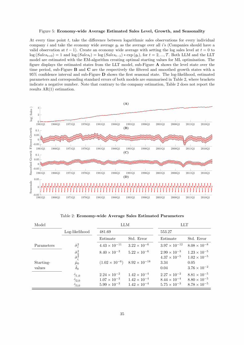
Figure 5: Economy-wide Average Estimated Sales Level, Growth, and Seasonality

At every time point t, take the difference between logarithmic sales observations for every individualcompany i and take the economy wide average gt as the average over all i’s (Companies should have avalid observation at t− 1). Create an economy wide average with setting the log sales level at t = 0 tolog (Salest=0) = 1 and log (Salest) = log (Salest−1) ∗ exp (gt), for t = 2, ..., T . Both LLM and the LLTmodel are estimated with the EM-algorithm creating optimal starting values for ML optimisation. Thefigure displays the estimated states from the LLT model, sub-Figure A shows the level state over thetime period, sub-Figure B and C are the respectively the filtered and smoothed growth states with a95% confidence interval and sub-Figure D shows the first seasonal state. The log-likelihood, estimatedparameters and corresponding standard errors of both models are summarised in Table 2, where bracketsindicate a negative number. Note that contrary to the company estimation, Table 2 does not report theresults AR(1) estimation.

Table 2: Economy-wide Average Sales Estimated Parameters

Model LLM LLT

Log-likelihood 481.69 553.27

Estimate Std. Error Estimate Std. Error

Parameters σ2ε 4.43× 10−11 3.22× 10−6 3.97× 10−12 8.08× 10−8

σ2η 8.40× 10−3 5.22× 10−6 2.99× 10−3 1.23× 10−5

σ2ζ 4.37× 10−5 1.02× 10−5

Starting- µ0 (1.02× 10−6) 8.92× 10−18 3.34 0.05

values δ0 0.04 3.76× 10−2

γ1,0 2.24× 10−2 1.42× 10−4 2.27× 10−2 8.81× 10−5

γ2,0 1.07× 10−3 1.42× 10−4 8.44× 10−4 8.80× 10−5

γ3,0 5.99× 10−3 1.42× 10−4 5.75× 10−3 8.78× 10−5

35

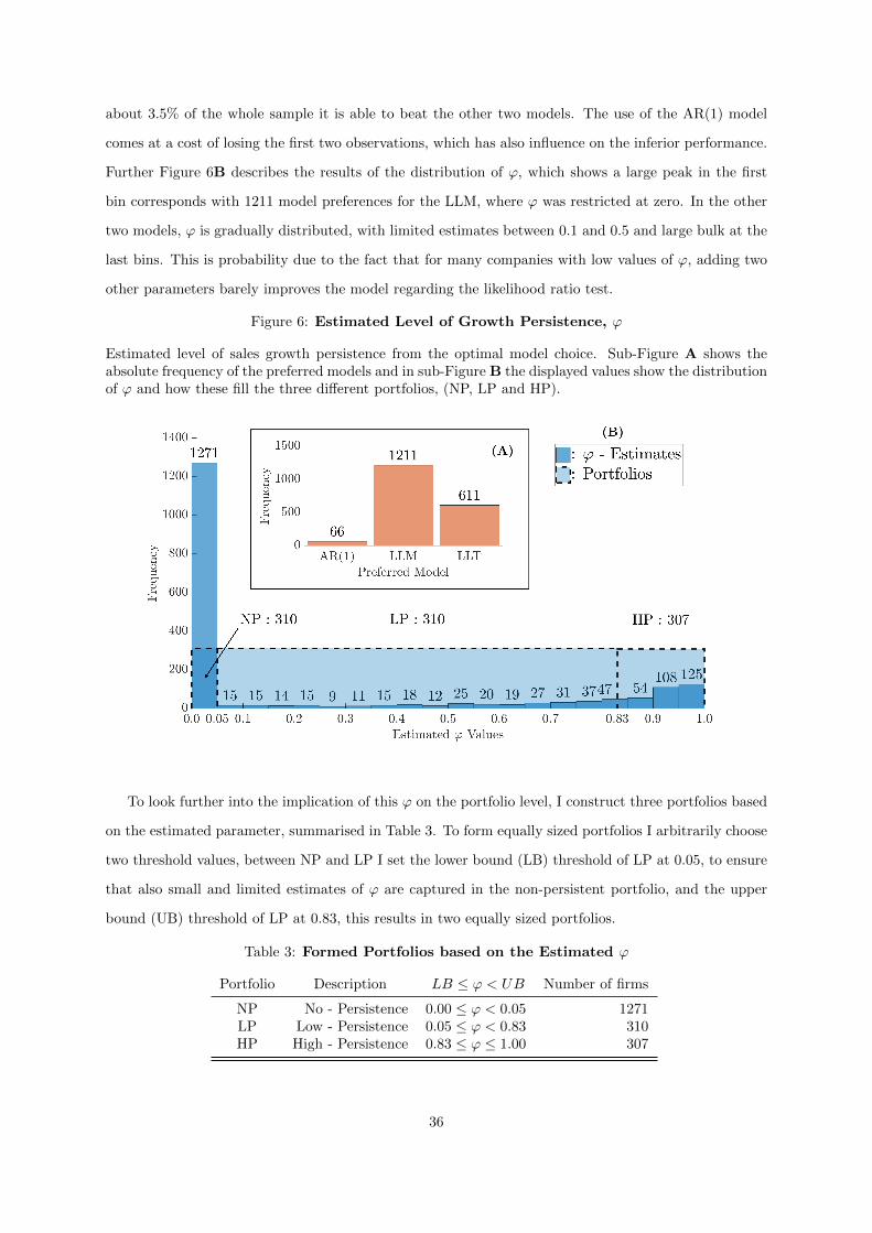
about 3.5% of the whole sample it is able to beat the other two models. The use of the AR(1) model

comes at a cost of losing the first two observations, which has also influence on the inferior performance.

Further Figure 6B describes the results of the distribution of ϕ, which shows a large peak in the first

bin corresponds with 1211 model preferences for the LLM, where ϕ was restricted at zero. In the other

two models, ϕ is gradually distributed, with limited estimates between 0.1 and 0.5 and large bulk at the

last bins. This is probability due to the fact that for many companies with low values of ϕ, adding two

other parameters barely improves the model regarding the likelihood ratio test.

Figure 6: Estimated Level of Growth Persistence, ϕ

Estimated level of sales growth persistence from the optimal model choice. Sub-Figure A shows theabsolute frequency of the preferred models and in sub-Figure B the displayed values show the distributionof ϕ and how these fill the three different portfolios, (NP, LP and HP).

To look further into the implication of this ϕ on the portfolio level, I construct three portfolios based

on the estimated parameter, summarised in Table 3. To form equally sized portfolios I arbitrarily choose

two threshold values, between NP and LP I set the lower bound (LB) threshold of LP at 0.05, to ensure

that also small and limited estimates of ϕ are captured in the non-persistent portfolio, and the upper

bound (UB) threshold of LP at 0.83, this results in two equally sized portfolios.

Table 3: Formed Portfolios based on the Estimated ϕ

Portfolio Description LB ≤ ϕ < UB Number of firms

NP No - Persistence 0.00 ≤ ϕ < 0.05 1271LP Low - Persistence 0.05 ≤ ϕ < 0.83 310HP High - Persistence 0.83 ≤ ϕ ≤ 1.00 307

36

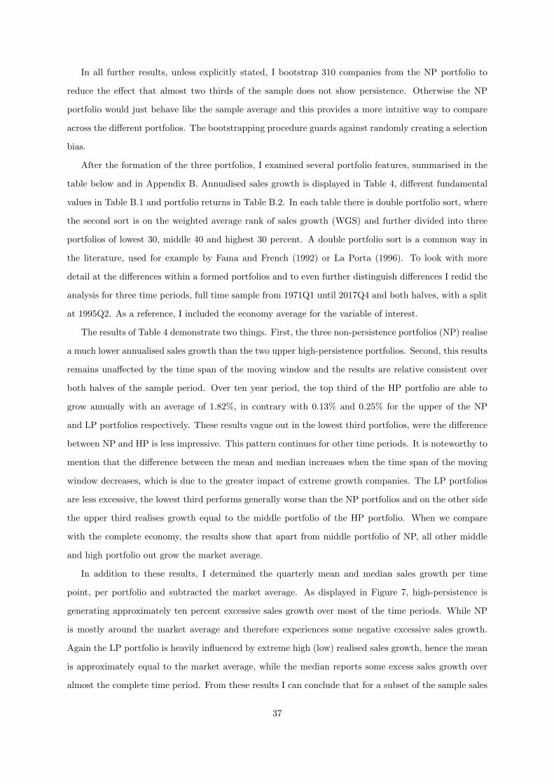
In all further results, unless explicitly stated, I bootstrap 310 companies from the NP portfolio to

reduce the effect that almost two thirds of the sample does not show persistence. Otherwise the NP

portfolio would just behave like the sample average and this provides a more intuitive way to compare

across the different portfolios. The bootstrapping procedure guards against randomly creating a selection

bias.

After the formation of the three portfolios, I examined several portfolio features, summarised in the

table below and in Appendix B. Annualised sales growth is displayed in Table 4, different fundamental

values in Table B.1 and portfolio returns in Table B.2. In each table there is double portfolio sort, where

the second sort is on the weighted average rank of sales growth (WGS) and further divided into three

portfolios of lowest 30, middle 40 and highest 30 percent. A double portfolio sort is a common way in

the literature, used for example by Fama and French (1992) or La Porta (1996). To look with more

detail at the differences within a formed portfolios and to even further distinguish differences I redid the

analysis for three time periods, full time sample from 1971Q1 until 2017Q4 and both halves, with a split

at 1995Q2. As a reference, I included the economy average for the variable of interest.

The results of Table 4 demonstrate two things. First, the three non-persistence portfolios (NP) realise

a much lower annualised sales growth than the two upper high-persistence portfolios. Second, this results

remains unaffected by the time span of the moving window and the results are relative consistent over

both halves of the sample period. Over ten year period, the top third of the HP portfolio are able to

grow annually with an average of 1.82%, in contrary with 0.13% and 0.25% for the upper of the NP

and LP portfolios respectively. These results vague out in the lowest third portfolios, were the difference

between NP and HP is less impressive. This pattern continues for other time periods. It is noteworthy to

mention that the difference between the mean and median increases when the time span of the moving

window decreases, which is due to the greater impact of extreme growth companies. The LP portfolios

are less excessive, the lowest third performs generally worse than the NP portfolios and on the other side

the upper third realises growth equal to the middle portfolio of the HP portfolio. When we compare

with the complete economy, the results show that apart from middle portfolio of NP, all other middle

and high portfolio out grow the market average.

In addition to these results, I determined the quarterly mean and median sales growth per time

point, per portfolio and subtracted the market average. As displayed in Figure 7, high-persistence is

generating approximately ten percent excessive sales growth over most of the time periods. While NP

is mostly around the market average and therefore experiences some negative excessive sales growth.

Again the LP portfolio is heavily influenced by extreme high (low) realised sales growth, hence the mean

is approximately equal to the market average, while the median reports some excess sales growth over

almost the complete time period. From these results I can conclude that for a subset of the sample sales

37

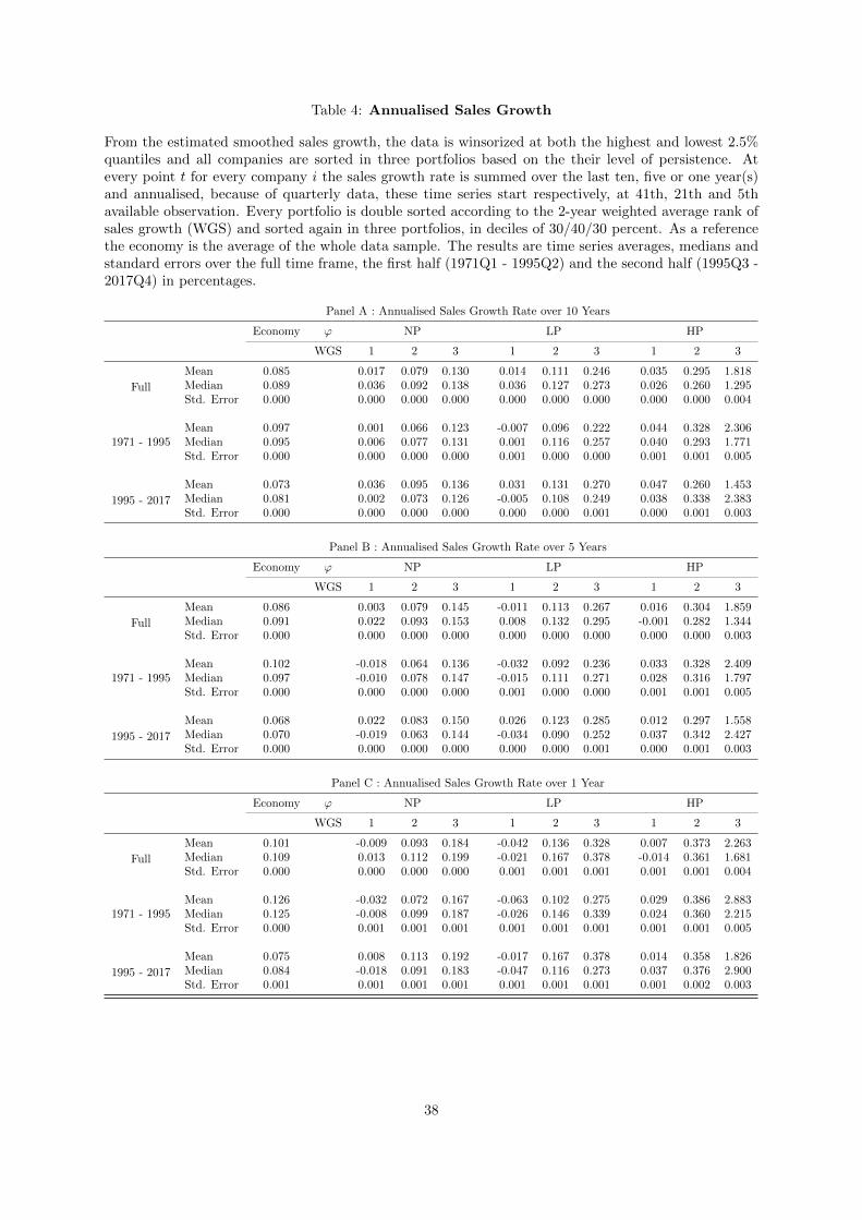
Table 4: Annualised Sales Growth

From the estimated smoothed sales growth, the data is winsorized at both the highest and lowest 2.5%quantiles and all companies are sorted in three portfolios based on the their level of persistence. Atevery point t for every company i the sales growth rate is summed over the last ten, five or one year(s)and annualised, because of quarterly data, these time series start respectively, at 41th, 21th and 5thavailable observation. Every portfolio is double sorted according to the 2-year weighted average rank ofsales growth (WGS) and sorted again in three portfolios, in deciles of 30/40/30 percent. As a referencethe economy is the average of the whole data sample. The results are time series averages, medians andstandard errors over the full time frame, the first half (1971Q1 - 1995Q2) and the second half (1995Q3 -2017Q4) in percentages.

Panel A : Annualised Sales Growth Rate over 10 Years

Economy ϕ NP LP HP

WGS 1 2 3 1 2 3 1 2 3

Full

Mean 0.085 0.017 0.079 0.130 0.014 0.111 0.246 0.035 0.295 1.818Median 0.089 0.036 0.092 0.138 0.036 0.127 0.273 0.026 0.260 1.295Std. Error 0.000 0.000 0.000 0.000 0.000 0.000 0.000 0.000 0.000 0.004

1971 - 1995Mean 0.097 0.001 0.066 0.123 -0.007 0.096 0.222 0.044 0.328 2.306Median 0.095 0.006 0.077 0.131 0.001 0.116 0.257 0.040 0.293 1.771Std. Error 0.000 0.000 0.000 0.000 0.001 0.000 0.000 0.001 0.001 0.005

1995 - 2017

Mean 0.073 0.036 0.095 0.136 0.031 0.131 0.270 0.047 0.260 1.453Median 0.081 0.002 0.073 0.126 -0.005 0.108 0.249 0.038 0.338 2.383Std. Error 0.000 0.000 0.000 0.000 0.000 0.000 0.001 0.000 0.001 0.003

Panel B : Annualised Sales Growth Rate over 5 Years

Economy ϕ NP LP HP

WGS 1 2 3 1 2 3 1 2 3

Full

Mean 0.086 0.003 0.079 0.145 -0.011 0.113 0.267 0.016 0.304 1.859Median 0.091 0.022 0.093 0.153 0.008 0.132 0.295 -0.001 0.282 1.344Std. Error 0.000 0.000 0.000 0.000 0.000 0.000 0.000 0.000 0.000 0.003

1971 - 1995Mean 0.102 -0.018 0.064 0.136 -0.032 0.092 0.236 0.033 0.328 2.409Median 0.097 -0.010 0.078 0.147 -0.015 0.111 0.271 0.028 0.316 1.797Std. Error 0.000 0.000 0.000 0.000 0.001 0.000 0.000 0.001 0.001 0.005

1995 - 2017

Mean 0.068 0.022 0.083 0.150 0.026 0.123 0.285 0.012 0.297 1.558Median 0.070 -0.019 0.063 0.144 -0.034 0.090 0.252 0.037 0.342 2.427Std. Error 0.000 0.000 0.000 0.000 0.000 0.000 0.001 0.000 0.001 0.003

Panel C : Annualised Sales Growth Rate over 1 Year

Economy ϕ NP LP HP

WGS 1 2 3 1 2 3 1 2 3

Full

Mean 0.101 -0.009 0.093 0.184 -0.042 0.136 0.328 0.007 0.373 2.263Median 0.109 0.013 0.112 0.199 -0.021 0.167 0.378 -0.014 0.361 1.681Std. Error 0.000 0.000 0.000 0.000 0.001 0.001 0.001 0.001 0.001 0.004

1971 - 1995Mean 0.126 -0.032 0.072 0.167 -0.063 0.102 0.275 0.029 0.386 2.883Median 0.125 -0.008 0.099 0.187 -0.026 0.146 0.339 0.024 0.360 2.215Std. Error 0.000 0.001 0.001 0.001 0.001 0.001 0.001 0.001 0.001 0.005

1995 - 2017

Mean 0.075 0.008 0.113 0.192 -0.017 0.167 0.378 0.014 0.358 1.826Median 0.084 -0.018 0.091 0.183 -0.047 0.116 0.273 0.037 0.376 2.900Std. Error 0.001 0.001 0.001 0.001 0.001 0.001 0.001 0.001 0.002 0.003

38

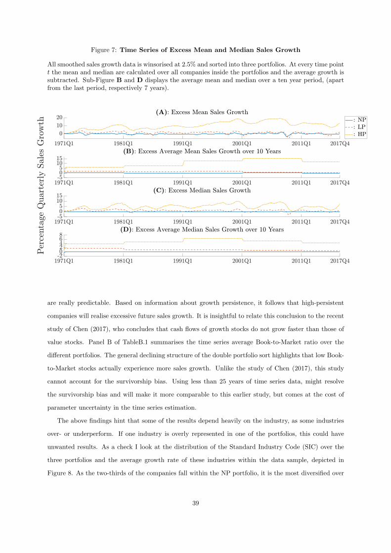
Figure 7: Time Series of Excess Mean and Median Sales Growth

All smoothed sales growth data is winsorised at 2.5% and sorted into three portfolios. At every time pointt the mean and median are calculated over all companies inside the portfolios and the average growth issubtracted. Sub-Figure B and D displays the average mean and median over a ten year period, (apartfrom the last period, respectively 7 years).

are really predictable. Based on information about growth persistence, it follows that high-persistent

companies will realise excessive future sales growth. It is insightful to relate this conclusion to the recent

study of Chen (2017), who concludes that cash flows of growth stocks do not grow faster than those of

value stocks. Panel B of TableB.1 summarises the time series average Book-to-Market ratio over the

different portfolios. The general declining structure of the double portfolio sort highlights that low Book-

to-Market stocks actually experience more sales growth. Unlike the study of Chen (2017), this study

cannot account for the survivorship bias. Using less than 25 years of time series data, might resolve

the survivorship bias and will make it more comparable to this earlier study, but comes at the cost of

parameter uncertainty in the time series estimation.

The above findings hint that some of the results depend heavily on the industry, as some industries

over- or underperform. If one industry is overly represented in one of the portfolios, this could have

unwanted results. As a check I look at the distribution of the Standard Industry Code (SIC) over the

three portfolios and the average growth rate of these industries within the data sample, depicted in

Figure 8. As the two-thirds of the companies fall within the NP portfolio, it is the most diversified over

39

all scale of industries and the LP and HP are a bit more clustered in specific industries. Concerning the

average growth of the industries, it comes clear that only a few reach far above the economy average, and

this mostly limits to small very specific industries and a small number of companies associated with it.

Therefore it can be easily rejected that high-persistence is an industry specific feature or that a cluster

of industries are accountable for large sales growth.

From an investors’ perspective it would be important to know if these persistent growth companies

are able to outperform the market by means of a positive return strategy. Following the same approach

as with the annualised sales growth, I calculate the annualised return rates over 10, 5 and 1 year(s),

with the double sort based on the WGS. Despite the idea that companies which encounter large sales

growth should have some kind of positive return, the data provides evidence that it is not the case. The

highest growing portfolio of the non persistent group performs similarly to the third sub-portfolio of the

high-persistent group. This is in line with evidence provided by Chan et al. (2003) and Chen (2017), who

also find that stocks with high revenue or earnings growth not necessarily excessive returns. Partially

this outcome corresponds to results of the analysis of the fundamentals of these double sorted portfolios.

The return rates are not corrected for basic asset pricing factors such as Value: High-Minus-Low, Size:

Small-Minus-Large or momentum, which might resolve any possible profitable strategy. Some minor

findings regarding the portfolio fundamentals are the decline in size and incline over Tobin’s Q Ratio

over all the first sorted portfolios, indicating that higher sales growth mainly occurs in growth companies

of which the market value exceeds to book value. Further panels with R&D, earnings and dividend per

share do not show such a straightforward pattern and the same goes for market equity. It is however

noteworthy to mention the high market equity value for the high-growth portfolio. A hypothesis for the

result might be that experiencing high past growth in sales will develop into a large market cap also this

further implies the strong affection by the survivorship bias. It would, on the other side at least be a

remarkable result as the first sort on sales persistence is a time invariant label. Many studies linking

fundamental numbers to returns do not approach this with permanent labels, but allow for time variation

in the explanatory variables.

40

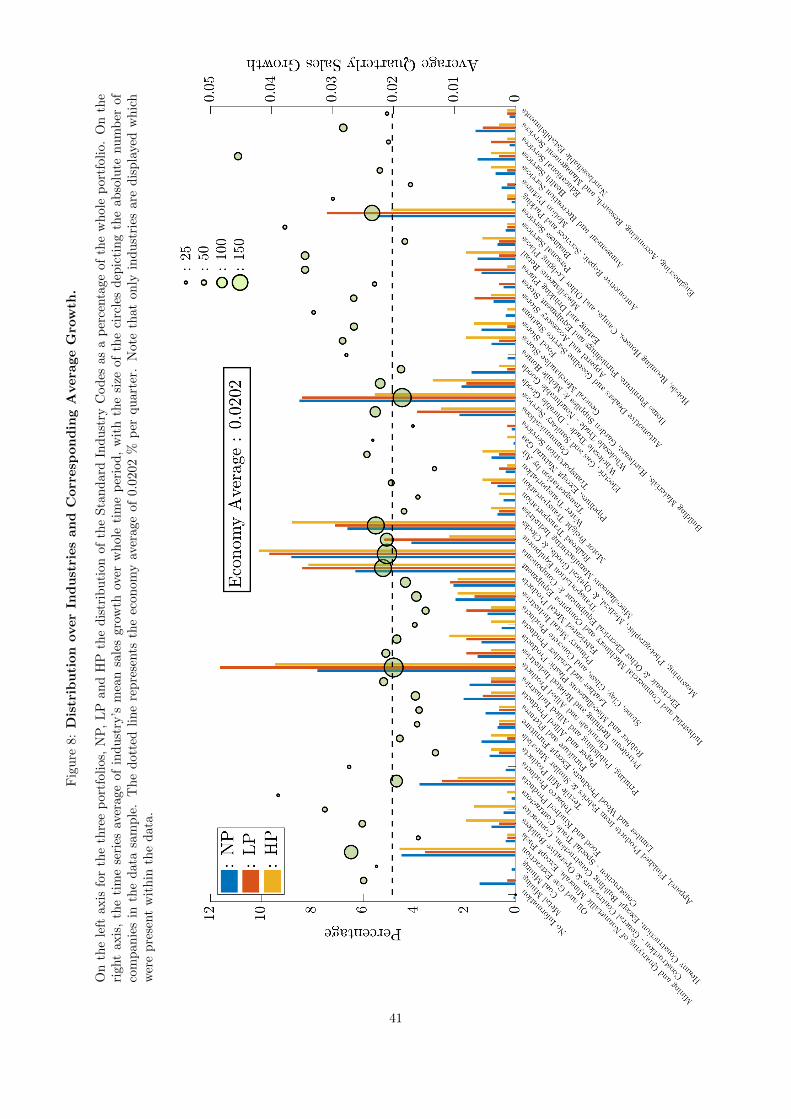
Fig

ure

8:D

istr

ibu

tion

over

Ind

ust

ries

an

dC

orr

esp

on

din

gA

vera

ge

Gro

wth

.

On

the

left

axis

for

the

thre

ep

ortf

olio

s,N

P,

LP

and

HP

the

dis

trib

uti

on

of

the

Sta

nd

ard

Ind

ust

ryC

od

esas

ap

erce

nta

ge

of

the

wh

ole

port

foli

o.

On

the

righ

tax

is,

the

tim

ese

ries

aver

age

ofin

du

stry

’sm

ean

sale

sgro

wth

over

wh

ole

tim

ep

erio

d,

wit

hth

esi

zeof

the

circ

les

dep

icti

ng

the

ab

solu

tenum

ber

of

com

pan

ies

inth

ed

ata

sam

ple

.T

he

dot

ted

lin

ere

pre

sents

the

econ

om

yav

erage

of

0.0

202

%p

erqu

art

er.

Note

that

on

lyin

du

stri

esare

dis

pla

yed

wh

ich

wer

ep

rese

nt

wit

hin

the

dat

a.

41

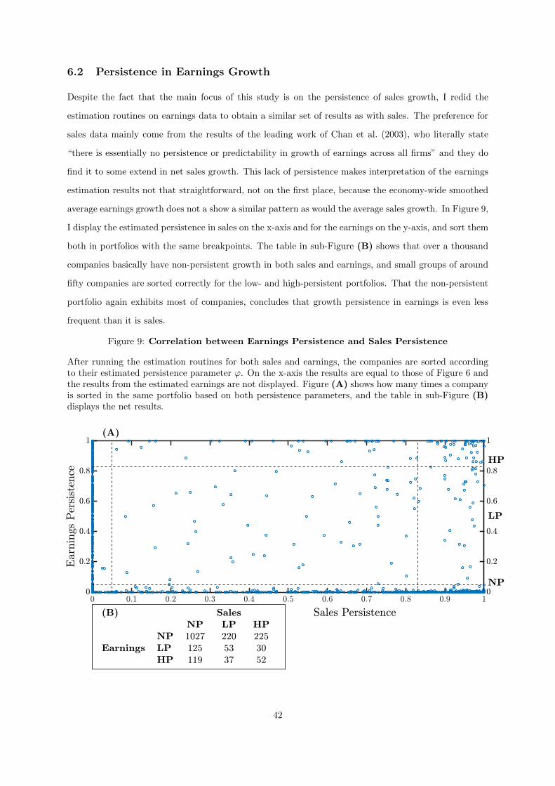
6.2 Persistence in Earnings Growth

Despite the fact that the main focus of this study is on the persistence of sales growth, I redid the

estimation routines on earnings data to obtain a similar set of results as with sales. The preference for

sales data mainly come from the results of the leading work of Chan et al. (2003), who literally state

“there is essentially no persistence or predictability in growth of earnings across all firms” and they do

find it to some extend in net sales growth. This lack of persistence makes interpretation of the earnings

estimation results not that straightforward, not on the first place, because the economy-wide smoothed

average earnings growth does not a show a similar pattern as would the average sales growth. In Figure 9,

I display the estimated persistence in sales on the x-axis and for the earnings on the y-axis, and sort them

both in portfolios with the same breakpoints. The table in sub-Figure (B) shows that over a thousand

companies basically have non-persistent growth in both sales and earnings, and small groups of around

fifty companies are sorted correctly for the low- and high-persistent portfolios. That the non-persistent

portfolio again exhibits most of companies, concludes that growth persistence in earnings is even less

frequent than it is sales.

Figure 9: Correlation between Earnings Persistence and Sales Persistence

After running the estimation routines for both sales and earnings, the companies are sorted accordingto their estimated persistence parameter ϕ. On the x-axis the results are equal to those of Figure 6 andthe results from the estimated earnings are not displayed. Figure (A) shows how many times a companyis sorted in the same portfolio based on both persistence parameters, and the table in sub-Figure (B)displays the net results.

42

6.3 Extrapolation Hypothesis

Before jumping into the estimation results of the different GARCH models with the many different

variables. I first examine if sign and magnitude of the created measure for sales surprises correlate with

the returns in an announcement week. Looking at the formal definition in post-earnings-announcement

drift literature, it is stated as the phenomenon that after a day of announcement, streaks of abnormal

returns accumulate in the direction of the surprise. Following this definition, the measure for earnings

surprise used most studies is the difference between the I/B/E/S analysts’ forecasts and the realised

earnings-per-share. Because this study is not using the common measure for the earnings surprise, but

the difference between observed sales and predicted sales from the Kalman filter, Equation 16, I conduct

the following to show that the sign and magnitude of this surprise also have a positive correlation with

the return in week of announcement, several weeks before the announcement and a couple of weeks

following the announcement. At a moment of announcement t∗ for company i, we know the sign of

the surprise, and returns for t∗ − 3 until t∗ + 8, where t is in weeks. A popular stylised fact for stock

returns is the absence of correlation between two periods, hence theoretically the correlation between t∗

and any other t∗ plus or minus a period should be zero. For every company I determine the correlation

matrix of the returns of t∗ − 3 until t∗ + 8 along with the correlation with the sign and magnitude of

the surprise. Table 5 summarises the Pearson’s correlation coefficients with the return of the moment of

an announcement, as many of the correlations between e.g. t∗ − 2 and t∗ + 4 are approximately zero. It

shows that the correlation between the announcement period and almost every other week is zero, apart

from the negative correlation with the week prior to the announcement and the sign and magnitude of the

surprise. Although the results are not extreme, this gives an indication to expect a certain relationship

between the returns at an announcement and the direction and size of the sales surprise.

Table 5: Correlation between Returns Around Announcement Period t∗

At every announcement period t∗, for every company i, determined the weekly returns for t∗ − 3 untilt∗ + 8 and the sign and magnitude of the sales surprise. Calculated the Pearson’s correlation matrixfor every company and summarised by means of the average, median and standard error. Only showingthe summary statistics of the correlation with the return of the announcement week t∗, therefore row t∗

is perfectly correlated. Note that Mean τ and Mean ρ are respectively the average of Kendall’s τ andSpearman’s ρ rank correlation coefficient and not all time period correlations are reported.

Mean Median Std. Er. (×1000) Mean τ Mean ρ

Magnitude 0.052 0.050 0.065 0.043 0.064Sign 0.051 0.048 0.064 0.045 0.055t∗ − 2 -0.001 -0.002 0.069 -0.004 -0.006t∗ − 1 -0.044 -0.047 0.075 -0.034 -0.049t∗ 1.00 1.00 0.00 1.00 1.00t∗ + 1 -0.010 -0.010 0.076 -0.008 -0.011t∗ + 2 0.019 0.017 0.071 0.014 0.020

43

When I alter the sales surprise measure to a more wider used scale, the difference between EPS∗t ,

and the EPSt∗−4, a year prior to the current announcement (Bernard and Thomas (1989)). It concludes

a similar pattern, apart from a higher correlation between the sign or magnitude and the return at

t∗, respectively 0.142 and 0.126 . Finding such a connection provides evidence that the sales surprise

measure I propose is not that distinct from the literature’s standard and hints on finding evidence of

PEAD.

Concluding that there is an indication that news does have an impact on the return and therefore

also volatility of stock prices, it opens the way to implement this into the GARCH framework. The

second set of results are obtained from the estimation routines for GARCH type models. For every

company this univariate approach produces ten estimated models, chosen from the optimal initialisation,

solely based on log-likelihood evaluation, mostly the differences are minor and an outcome of numerical

discrepancies. Out of the ten estimated models I neglect the ones where the exogenous parameter(s)

estimate(s)are insignificant at 5% level, as all other GARCH estimates are significant for most of the

companies. When I compare different models in such a case, I always choose the model without the

addition of an extra variable. Table 6 displays the cases where the coefficient of the exogenous variable

is insignificant between brackets. For example, when I compare model preferences between the basic

GARCH model and the addition of X1, for 399 companies the parameter is insignificant, hence only for

578 companies adding X1 does not directly improve the fit to the data. This explains why the base case

model, is not preferred for a fixed amount of companies, for every model set, a different number of models

has insignificant parameters. Another example, adding X1 leaves 399 companies and in which cases the

base case is always preferred, and so only adding X2 excludes more than 322 companies, but when we

compare the set, base case, X1 and X2, only 183 companies are left out of the sample, showing a minor

inclusion of the number of models that have insignificant parameters for both exogenous variables.

Table 6: GARCH Optimal Model Preferences

Based on the AIC, the numbers display the times that a certain model is optimal above the base set X0or other models in the set. The number between brackets in the first column is the sum of the number ofmodels at which the exogenous parameters is insignificant at a 5% level, so where the base case alwaysis optimal model. Only relevant models sets are displayed.

GARCH GJR

Model Set X0 X1 X2 X3 X4 X0 X1 X2 X3 X4

1. X1 977 ( 399 ) 911 948 ( 363 ) 9402. X2 1015 ( 322 ) 873 980 ( 318 ) 9083. X3 1145 ( 646 ) 743 1092 ( 592 ) 7964. X4 1127 ( 366 ) 761 1089 ( 351 ) 7995. X1 - X2 781 ( 183 ) 640 467 750 ( 172 ) 638 5006. X1 - X3 836 ( 262 ) 663 389 788 ( 237 ) 657 4437. X2 - X3 950 ( 276 ) 550 388 913 ( 270 ) 547 4288. X2 - X4 943 ( 241 ) 634 311 905 ( 231 ) 655 3289. X1 - X2 - X3 - X4 698 ( 130 ) 562 206 183 239 662 ( 10 ) 561 217 211 237

44

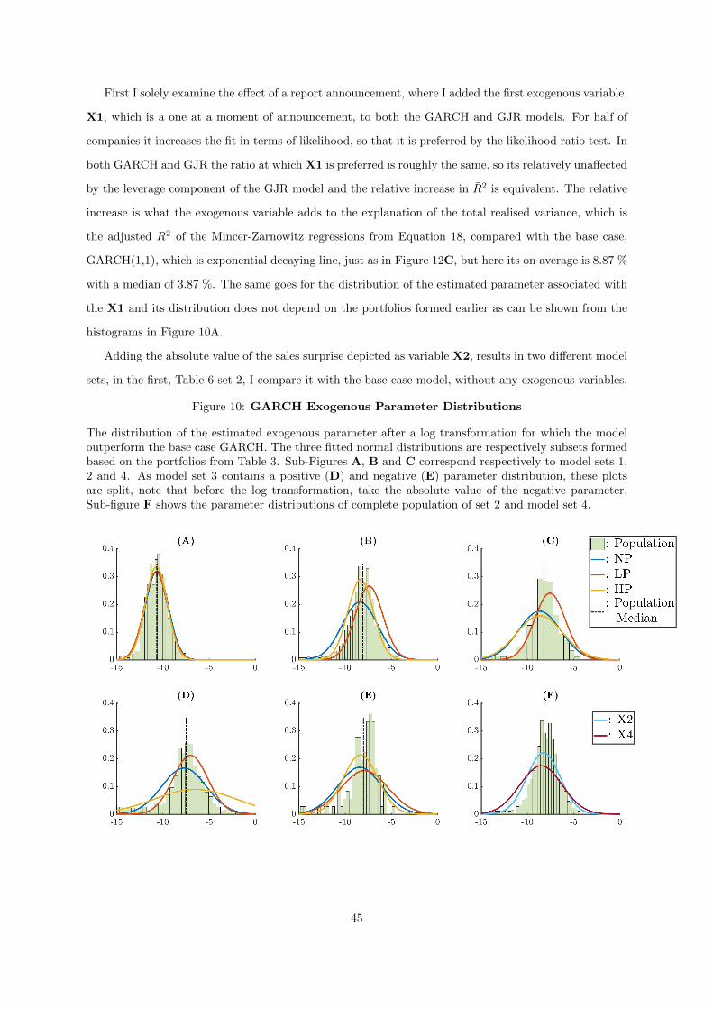
First I solely examine the effect of a report announcement, where I added the first exogenous variable,

X1, which is a one at a moment of announcement, to both the GARCH and GJR models. For half of

companies it increases the fit in terms of likelihood, so that it is preferred by the likelihood ratio test. In

both GARCH and GJR the ratio at which X1 is preferred is roughly the same, so its relatively unaffected

by the leverage component of the GJR model and the relative increase in R2 is equivalent. The relative

increase is what the exogenous variable adds to the explanation of the total realised variance, which is

the adjusted R2 of the Mincer-Zarnowitz regressions from Equation 18, compared with the base case,

GARCH(1,1), which is exponential decaying line, just as in Figure 12C, but here its on average is 8.87 %

with a median of 3.87 %. The same goes for the distribution of the estimated parameter associated with

the X1 and its distribution does not depend on the portfolios formed earlier as can be shown from the

histograms in Figure 10A.

Adding the absolute value of the sales surprise depicted as variable X2, results in two different model

sets, in the first, Table 6 set 2, I compare it with the base case model, without any exogenous variables.

Figure 10: GARCH Exogenous Parameter Distributions

The distribution of the estimated exogenous parameter after a log transformation for which the modeloutperform the base case GARCH. The three fitted normal distributions are respectively subsets formedbased on the portfolios from Table 3. Sub-Figures A, B and C correspond respectively to model sets 1,2 and 4. As model set 3 contains a positive (D) and negative (E) parameter distribution, these plotsare split, note that before the log transformation, take the absolute value of the negative parameter.Sub-figure F shows the parameter distributions of complete population of set 2 and model set 4.

45

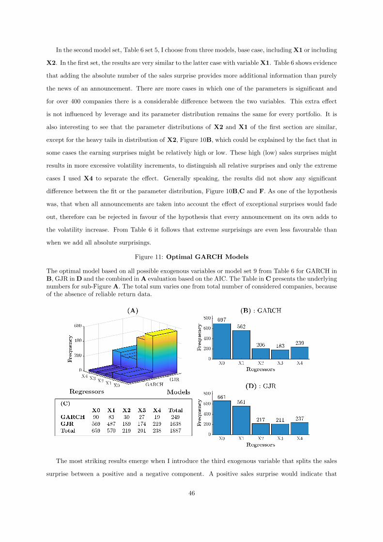
In the second model set, Table 6 set 5, I choose from three models, base case, including X1 or including

X2. In the first set, the results are very similar to the latter case with variable X1. Table 6 shows evidence

that adding the absolute number of the sales surprise provides more additional information than purely

the news of an announcement. There are more cases in which one of the parameters is significant and

for over 400 companies there is a considerable difference between the two variables. This extra effect

is not influenced by leverage and its parameter distribution remains the same for every portfolio. It is

also interesting to see that the parameter distributions of X2 and X1 of the first section are similar,

except for the heavy tails in distribution of X2, Figure 10B, which could be explained by the fact that in

some cases the earning surprises might be relatively high or low. These high (low) sales surprises might

results in more excessive volatility increments, to distinguish all relative surprises and only the extreme

cases I used X4 to separate the effect. Generally speaking, the results did not show any significant

difference between the fit or the parameter distribution, Figure 10B,C and F. As one of the hypothesis

was, that when all announcements are taken into account the effect of exceptional surprises would fade

out, therefore can be rejected in favour of the hypothesis that every announcement on its own adds to

the volatility increase. From Table 6 it follows that extreme surprisings are even less favourable than

when we add all absolute surprisings.

Figure 11: Optimal GARCH Models

The optimal model based on all possible exogenous variables or model set 9 from Table 6 for GARCH inB, GJR in D and the combined in A evaluation based on the AIC. The Table in C presents the underlyingnumbers for sub-Figure A. The total sum varies one from total number of considered companies, becauseof the absence of reliable return data.

The most striking results emerge when I introduce the third exogenous variable that splits the sales

surprise between a positive and a negative component. A positive sales surprise would indicate that

46

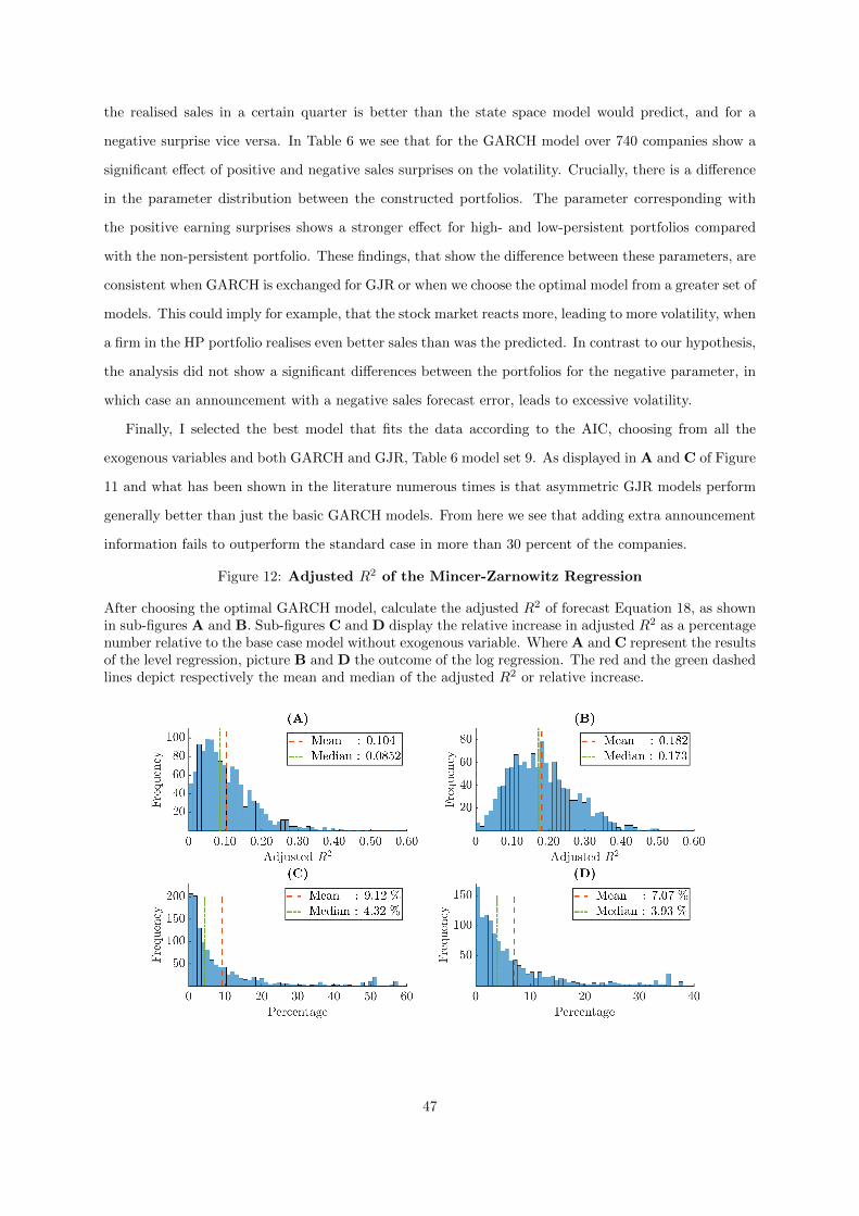
the realised sales in a certain quarter is better than the state space model would predict, and for a

negative surprise vice versa. In Table 6 we see that for the GARCH model over 740 companies show a

significant effect of positive and negative sales surprises on the volatility. Crucially, there is a difference

in the parameter distribution between the constructed portfolios. The parameter corresponding with

the positive earning surprises shows a stronger effect for high- and low-persistent portfolios compared

with the non-persistent portfolio. These findings, that show the difference between these parameters, are

consistent when GARCH is exchanged for GJR or when we choose the optimal model from a greater set of

models. This could imply for example, that the stock market reacts more, leading to more volatility, when

a firm in the HP portfolio realises even better sales than was the predicted. In contrast to our hypothesis,

the analysis did not show a significant differences between the portfolios for the negative parameter, in

which case an announcement with a negative sales forecast error, leads to excessive volatility.

Finally, I selected the best model that fits the data according to the AIC, choosing from all the

exogenous variables and both GARCH and GJR, Table 6 model set 9. As displayed in A and C of Figure

11 and what has been shown in the literature numerous times is that asymmetric GJR models perform

generally better than just the basic GARCH models. From here we see that adding extra announcement

information fails to outperform the standard case in more than 30 percent of the companies.

Figure 12: Adjusted R2 of the Mincer-Zarnowitz Regression

After choosing the optimal GARCH model, calculate the adjusted R2 of forecast Equation 18, as shownin sub-figures A and B. Sub-figures C and D display the relative increase in adjusted R2 as a percentagenumber relative to the base case model without exogenous variable. Where A and C represent the resultsof the level regression, picture B and D the outcome of the log regression. The red and the green dashedlines depict respectively the mean and median of the adjusted R2 or relative increase.

47

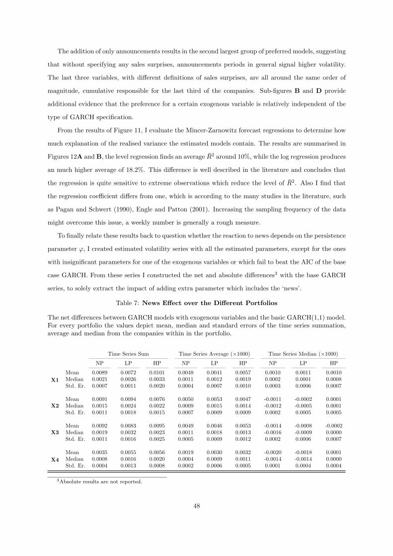
The addition of only announcements results in the second largest group of preferred models, suggesting

that without specifying any sales surprises, announcements periods in general signal higher volatility.

The last three variables, with different definitions of sales surprises, are all around the same order of

magnitude, cumulative responsible for the last third of the companies. Sub-figures B and D provide

additional evidence that the preference for a certain exogenous variable is relatively independent of the

type of GARCH specification.

From the results of Figure 11, I evaluate the Mincer-Zarnowitz forecast regressions to determine how

much explanation of the realised variance the estimated models contain. The results are summarised in

Figures 12A and B, the level regression finds an average R2 around 10%, while the log regression produces

an much higher average of 18.2%. This difference is well described in the literature and concludes that

the regression is quite sensitive to extreme observations which reduce the level of R2. Also I find that

the regression coefficient differs from one, which is according to the many studies in the literature, such

as Pagan and Schwert (1990), Engle and Patton (2001). Increasing the sampling frequency of the data

might overcome this issue, a weekly number is generally a rough measure.

To finally relate these results back to question whether the reaction to news depends on the persistence

parameter ϕ, I created estimated volatility series with all the estimated parameters, except for the ones

with insignificant parameters for one of the exogenous variables or which fail to beat the AIC of the base

case GARCH. From these series I constructed the net and absolute differences3 with the base GARCH

series, to solely extract the impact of adding extra parameter which includes the ‘news’.

Table 7: News Effect over the Different Portfolios

The net differences between GARCH models with exogenous variables and the basic GARCH(1,1) model.For every portfolio the values depict mean, median and standard errors of the time series summation,average and median from the companies within in the portfolio.

Time Series Sum Time Series Average (×1000) Time Series Median (×1000)

NP LP HP NP LP HP NP LP HP

X1

Mean 0.0089 0.0072 0.0101 0.0048 0.0041 0.0057 0.0010 0.0011 0.0010Median 0.0021 0.0026 0.0033 0.0011 0.0012 0.0019 0.0002 0.0001 0.0008Std. Er. 0.0007 0.0011 0.0020 0.0004 0.0007 0.0010 0.0003 0.0006 0.0007

X2Mean 0.0091 0.0094 0.0076 0.0050 0.0053 0.0047 -0.0011 -0.0002 0.0001Median 0.0015 0.0024 0.0022 0.0009 0.0015 0.0014 -0.0012 -0.0005 0.0001Std. Er. 0.0011 0.0018 0.0015 0.0007 0.0009 0.0009 0.0002 0.0005 0.0005

X3Mean 0.0092 0.0083 0.0095 0.0049 0.0046 0.0053 -0.0014 -0.0008 -0.0002Median 0.0019 0.0032 0.0023 0.0011 0.0018 0.0013 -0.0016 -0.0009 0.0000Std. Er. 0.0011 0.0016 0.0025 0.0005 0.0009 0.0012 0.0002 0.0006 0.0007

X4

Mean 0.0035 0.0055 0.0056 0.0019 0.0030 0.0032 -0.0020 -0.0018 0.0001Median 0.0008 0.0016 0.0020 0.0004 0.0009 0.0011 -0.0014 -0.0014 0.0000Std. Er. 0.0004 0.0013 0.0008 0.0002 0.0006 0.0005 0.0001 0.0004 0.0004

3Absolute results are not reported.

48

In the theoretical scenario, the other parameter estimates vary minimal from the base case. For

every company, I summarise these differences by total sum, time series average and median and examine

their portfolio summary statistics displayed in Table 7. Although it might seem that the HP portfolio in

general has a higher response to news, it is hard to find a significant differences among the portfolios, not

least, because of large differences between individual companies. To overcome this, I also reported the

median of the distribution to news effects, in which the parallel between portfolios is hard to distinguish.

These results indicate that there are negligible differences between the reaction to announcement news

among the different portfolios. Finding a possible explanation in the fact that the portfolio sort on

persistence can not expose significant differences in news reactions.

6.4 Case Study: Apple Inc. vs. Ford Motor Company

In this section I perform a case study to elaborate on the estimation results and robustness, and provide

illustrative figures that address similarities and differences. I choose two large, well-known U.S. based

companies that come from a completely different industry, Apple Inc. and Ford Motor Company.

Where the first is one of the major producer of consumer electronics and the latter is the fifth largest

car manufacturer of the world.

Table 8: Case Study: Sales Growth Estimation Results

A summary of the of estimation results evaluating the quarterly sales of Panel A, Apple and PanelB, Ford with three different models and three different techniques for each model. EM stands forthe Expectation Maximisation method, the two different ML (Maximum Likelihood) methods, havea different initialisation, the first uses the EM as prior and the second column starts with a diffuseprior. The AR(1) model display one column with OLS regression estimates and and two columns with(Un)Restricted state space estimates, in which ϕ is restricted between zero and one. All models andtechniques are further described in the Section 5. LogL represents the score of the log likelihood function,ϕ the persistence parameter, and further contains the three state variance terms.

Panel A: Apple

LLM LLT AR(1)

EM ML EM ML Regression Restricted Unrestricted

LogL 36.04 64.49 64.48 33.29 63.44 69.49 22.85 20.29 22.85ϕ -0.257 0.000 0.934 -0.185 0.000 -0.188σ2ε 0.026 0.003 0.003 0.000 0.003 0.008σ2η 0.022 0.018 0.018 0.037 0.000 0.007σ2ζ 0.033 0.018 0.000 0.043 0.044 0.043

Panel B: Ford

LLM LLT AR(1)

EM ML EM ML Regression Restricted Unrestricted

LogL 164.63 223.71 223.09 175.80 222.04 221.97 145.51 116.31 145.51ϕ -0.993 0.000 0.000 -0.486 0.000 -0.481σ2ε 0.017 0.003 0.003 0.000 0.003 0.003σ2η 0.002 0.003 0.003 0.019 0.000 0.002σ2ζ 0.000 0.003 0.002 0.016 0.021 0.016

49

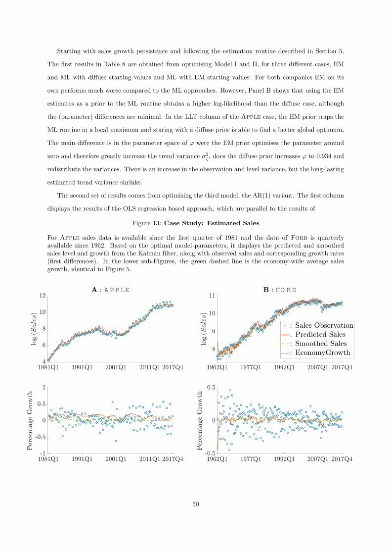
Starting with sales growth persistence and following the estimation routine described in Section 5.

The first results in Table 8 are obtained from optimising Model I and II, for three different cases, EM

and ML with diffuse starting values and ML with EM starting values. For both companies EM on its

own performs much worse compared to the ML approaches. However, Panel B shows that using the EM

estimates as a prior to the ML routine obtains a higher log-likelihood than the diffuse case, although

the (parameter) differences are minimal. In the LLT column of the Apple case, the EM prior traps the

ML routine in a local maximum and staring with a diffuse prior is able to find a better global optimum.

The main difference is in the parameter space of ϕ were the EM prior optimises the parameter around

zero and therefore greatly increase the trend variance σ2ζ , does the diffuse prior increases ϕ to 0.934 and

redistribute the variances. There is an increase in the observation and level variance, but the long-lasting

estimated trend variance shrinks.

The second set of results comes from optimising the third model, the AR(1) variant. The first column

displays the results of the OLS regression based approach, which are parallel to the results of

Figure 13: Case Study: Estimated Sales

For Apple sales data is available since the first quarter of 1981 and the data of Ford is quarterlyavailable since 1962. Based on the optimal model parameters, it displays the predicted and smoothedsales level and growth from the Kalman filter, along with observed sales and corresponding growth rates(first differences). In the lower sub-Figures, the green dashed line is the economy-wide average salesgrowth, identical to Figure 5.

A PPLE FO R D

50

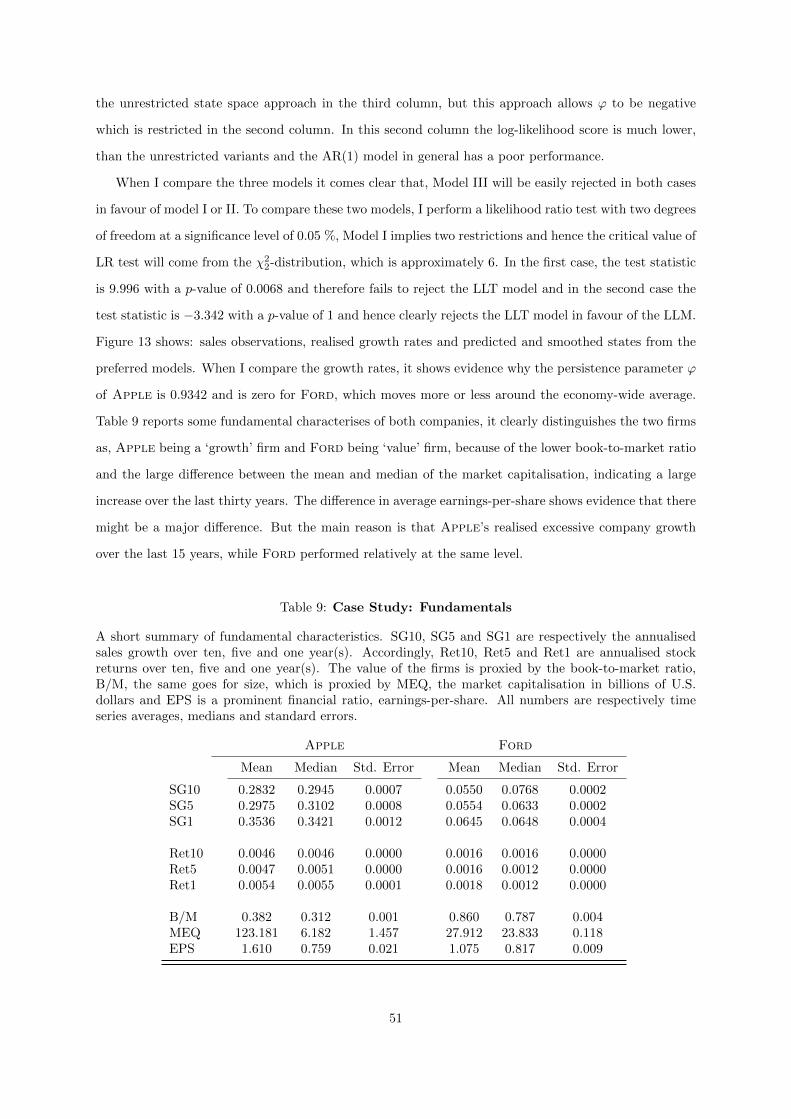
the unrestricted state space approach in the third column, but this approach allows ϕ to be negative

which is restricted in the second column. In this second column the log-likelihood score is much lower,

than the unrestricted variants and the AR(1) model in general has a poor performance.

When I compare the three models it comes clear that, Model III will be easily rejected in both cases

in favour of model I or II. To compare these two models, I perform a likelihood ratio test with two degrees

of freedom at a significance level of 0.05 %, Model I implies two restrictions and hence the critical value of

LR test will come from the χ22-distribution, which is approximately 6. In the first case, the test statistic

is 9.996 with a p-value of 0.0068 and therefore fails to reject the LLT model and in the second case the

test statistic is −3.342 with a p-value of 1 and hence clearly rejects the LLT model in favour of the LLM.

Figure 13 shows: sales observations, realised growth rates and predicted and smoothed states from the

preferred models. When I compare the growth rates, it shows evidence why the persistence parameter ϕ

of Apple is 0.9342 and is zero for Ford, which moves more or less around the economy-wide average.

Table 9 reports some fundamental characterises of both companies, it clearly distinguishes the two firms

as, Apple being a ‘growth’ firm and Ford being ‘value’ firm, because of the lower book-to-market ratio

and the large difference between the mean and median of the market capitalisation, indicating a large

increase over the last thirty years. The difference in average earnings-per-share shows evidence that there

might be a major difference. But the main reason is that Apple’s realised excessive company growth

over the last 15 years, while Ford performed relatively at the same level.

Table 9: Case Study: Fundamentals

A short summary of fundamental characteristics. SG10, SG5 and SG1 are respectively the annualisedsales growth over ten, five and one year(s). Accordingly, Ret10, Ret5 and Ret1 are annualised stockreturns over ten, five and one year(s). The value of the firms is proxied by the book-to-market ratio,B/M, the same goes for size, which is proxied by MEQ, the market capitalisation in billions of U.S.dollars and EPS is a prominent financial ratio, earnings-per-share. All numbers are respectively timeseries averages, medians and standard errors.

Apple Ford

Mean Median Std. Error Mean Median Std. Error

SG10 0.2832 0.2945 0.0007 0.0550 0.0768 0.0002SG5 0.2975 0.3102 0.0008 0.0554 0.0633 0.0002SG1 0.3536 0.3421 0.0012 0.0645 0.0648 0.0004

Ret10 0.0046 0.0046 0.0000 0.0016 0.0016 0.0000Ret5 0.0047 0.0051 0.0000 0.0016 0.0012 0.0000Ret1 0.0054 0.0055 0.0001 0.0018 0.0012 0.0000

B/M 0.382 0.312 0.001 0.860 0.787 0.004MEQ 123.181 6.182 1.457 27.912 23.833 0.118EPS 1.610 0.759 0.021 1.075 0.817 0.009

51

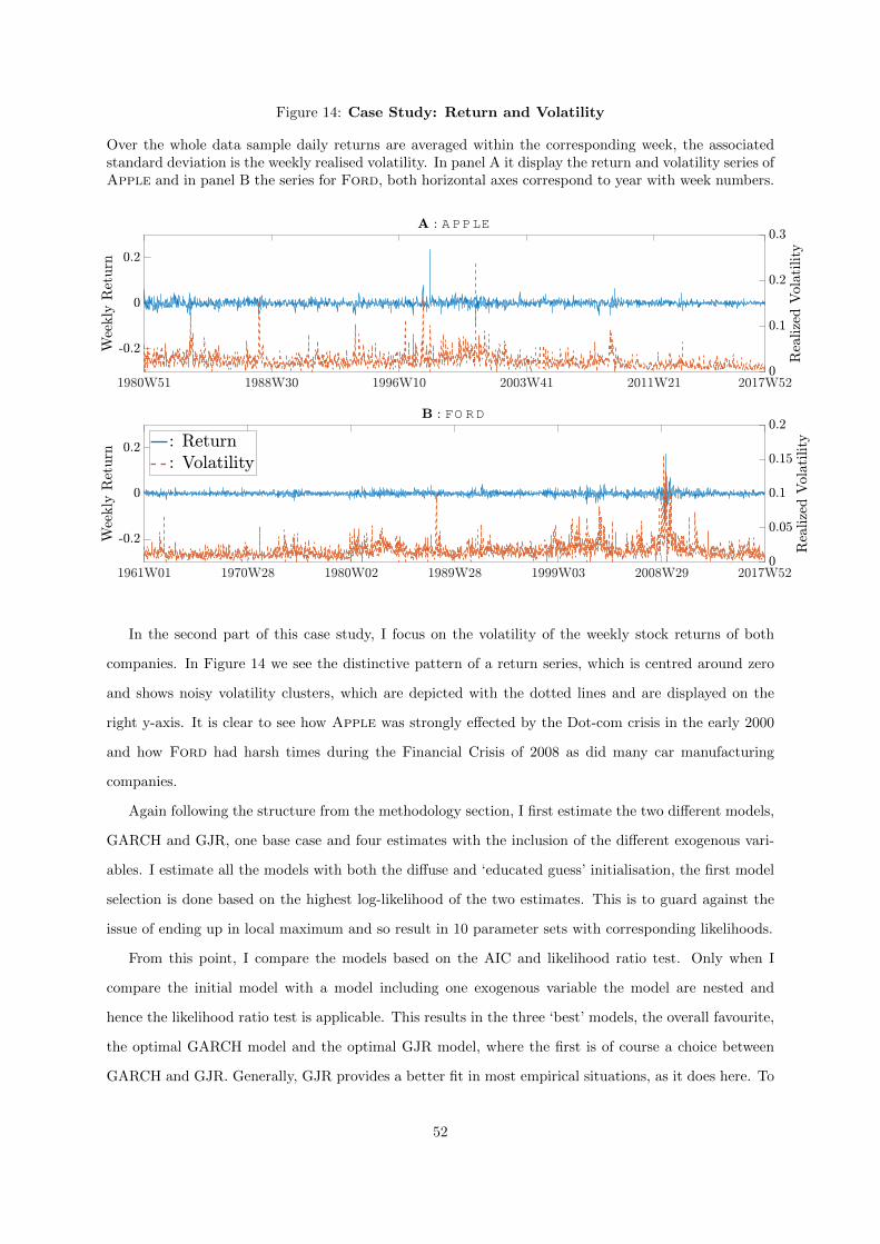
Figure 14: Case Study: Return and Volatility

Over the whole data sample daily returns are averaged within the corresponding week, the associatedstandard deviation is the weekly realised volatility. In panel A it display the return and volatility series ofApple and in panel B the series for Ford, both horizontal axes correspond to year with week numbers.

A PPLE

FO R D

In the second part of this case study, I focus on the volatility of the weekly stock returns of both

companies. In Figure 14 we see the distinctive pattern of a return series, which is centred around zero

and shows noisy volatility clusters, which are depicted with the dotted lines and are displayed on the

right y-axis. It is clear to see how Apple was strongly effected by the Dot-com crisis in the early 2000

and how Ford had harsh times during the Financial Crisis of 2008 as did many car manufacturing

companies.

Again following the structure from the methodology section, I first estimate the two different models,

GARCH and GJR, one base case and four estimates with the inclusion of the different exogenous vari-

ables. I estimate all the models with both the diffuse and ‘educated guess’ initialisation, the first model

selection is done based on the highest log-likelihood of the two estimates. This is to guard against the

issue of ending up in local maximum and so result in 10 parameter sets with corresponding likelihoods.

From this point, I compare the models based on the AIC and likelihood ratio test. Only when I

compare the initial model with a model including one exogenous variable the model are nested and

hence the likelihood ratio test is applicable. This results in the three ‘best’ models, the overall favourite,

the optimal GARCH model and the optimal GJR model, where the first is of course a choice between

GARCH and GJR. Generally, GJR provides a better fit in most empirical situations, as it does here. To

52

compare both companies, I only report the estimation results of the base model and the addition of the

first two exogenous variables, which correspond to a unit vector at the moment of announcement and

the absolute sales surprise. Table 10 is split into four panels, panel A shows the estimation results of

the three GARCH models and corresponding standard errors, likewise panel C adds the leverage effect,

encapsulated in the GJR models, and displays the corresponding estimated values and standard errors.

Panel B and D present the results of the Mincer-Zarnowitz regression of the estimated models on the

realised volatility, with intercept a and slope coefficient b. As previous studies mentioned, the theoretical

values of a = 0 and b = 1 are again violated in this case study, most likely due to the rough measure

of the realised volatility. The measure of explained variance in regressions, R2, we see the empirical

preference for the log version, because it is less sensitive to extreme observations. From the AIC we see

that the GJR models is preferred in favour of the standard GARCH model and the addition of extra

announcement variable adds just a little bit to the overall explained variance. Despite that the results

seem minor, based on the GJR case, for Apple the first exogenous variable adds 6.7% and 2.1% to R2

of the level and log regression and regarding X2 it adds 2.2% and 1.7% and in the same way, in the

Ford case it adds 0.5% and 1.8% for X1 to the explained realised variance and roughly the same for

the second variable.

Table 10: Case Study: GARCH Estimation Results

Estimation results and standard errors for GARCH and GJR with and without the first two exogenousvariables, X1 and X2 in Panel A and C, p-values are not reported, but are all smaller than 0.01. PanelB and D report the estimation results of the Mincer-Zarnowitz regression with HAC standard errors,along with the adjusted R2 of both the level and log regression and the Akaike Information Criteria.

Apple Ford

GARCH GARCH-X1 GARCH-X2 GARCH GARCH-X1 GARCH-X2

Panel A Est. SE Est. SE Est. SE Est. SE Est. SE Est. SE

ω 5.693× 10−7 7.976× 10−10 2.918× 10−9 3.447× 10−11 2.784× 10−8 4.865× 10−10 1.094× 10−6 1.123× 10−10 1.026× 10−6 9.847× 10−11 1.018× 10−6 1.091× 10−10

β1 0.952 6.497× 10−8 0.943 1.503× 10−7 0.954 1.156× 10−7 0.918 6.632× 10−7 0.917 6.914× 10−7 0.918 6.676× 10−7

λ1 0.047 1.121× 10−7 0.057 4.139× 10−8 0.046 9.801× 10−10 0.069 1.170× 10−6 0.069 1.329× 10−6 0.068 1.283× 10−6

γ1 9.355× 10−6 2.364× 10−9 3.109× 10−4 5.674× 10−9 2.431× 10−6 1.934× 10−9 3.066× 10−4 7.494× 10−8

Panel B

a 3.022× 10−4 1.126× 10−4 3.278× 10−4 1.180× 10−4 2.984× 10−4 1.124× 10−4 2.079× 10−4 3, 874× 10−5 2.064× 10−4 3.912× 10−5 2.056× 10−4 3.917× 10−5

b 2.996 0.730 2.783 0.738 2.953 0.713 2.103 0.498 2.119 0.503 2.128 0.504Level : R2 0.035 0.035 0.036 0.191 0.191 0.191

Log : R2 0.239 AIC : -11608 0.243 AIC : -11608 0.245 AIC : -11608 0.221 AIC : -20217 0.224 AIC : -20216 0.224 AIC : -20217

Apple Ford

GJR GJR-X1 GJR-X2 GJR GJR-X1 GJR-X2

Panel C Est. SE Est. SE Est. SE Est. SE Est. SE Est. SE

ω 6.440× 10−7 6.093× 10−10 1.881× 10−8 6.514× 10−10 1.483× 10−7 4.1369× 10−10 8.047× 10−7 1.263× 10−10 7.054× 10−7 9.961× 10−12 7.503× 10−7 1.176× 10−10

β1 0.950 7.605× 10−9 0.936 3.486× 10−14 0.952 3.329× 10−11 0.930 5.771× 10−7 0.929 5.985× 10−7 0.930 5.872× 10−7

λ1 0.029 1.023× 10−6 0.037 8.715× 10−13 0.029 5.481× 10−7 0.028 1.615× 10−6 0.028 1.747× 10−6 0.028 1.692× 10−6

λ2 0.039 1.712× 10−6 0.053 6.163× 10−13 0.037 1.201× 10−6 0.066 3.353× 10−6 0.068 3.478× 10−6 0.067 3.417× 10−6

γ1 1.263× 10−5 2.583× 10−9 2.727× 10−4 6.024× 10−8 2.743× 10−6 1.667× 10−9 2.397× 10−4 6.627× 10−8

Panel D

a 1.489× 10−4 8.419× 10−5 1.677× 10−4 8.875× 10−5 1.525× 10−4 8.372× 10−5 1.629× 10−4 4.527× 10−5 1.605× 10−4 4.569× 10−5 1.599× 10−4 4.597× 10−5

b 3.940 0.627 3.710 0.627 3.852 0.611 2.670 0.599 2.683 0.601 2.697 0.606Level : R2 0.045 0.048 0.046 0.223 0.224 0.224

Log : R2 0.243 AIC : -11618 0.248 AIC : -11620 0.247 AIC : -11618 0.225 AIC : -20256 0.229 AIC : -20256 0.229 AIC : -20256

53

As a final aspect to look at the differences between Apple and Ford I plot the time series of the

estimated GJR models in Figure 15, along with realised volatility and the difference between both the

GJR models for both companies. The black asterisks indicate a announcement moment. In panel C of

Table 10, we see that the estimate of γ1 for both companies differs by a factor 4, which implies that

Apple’s reaction to news announcements results in four times more volatility than it would with Ford.

The more structured pattern in the bottom figure of Apple indicates that the estimated parameters with

GJR-X2 do not vary much from the base case GJR, and so nicely extract the news effect. To further

extend this claim, I compare this different parameter estimates for the second exogenous variable, here

the estimates are more in the same order of magnitude. The question is whether this also results into a

similar reaction to the absolute sales surprise, as the latter could vary a lot per announcement and also

per company. Table 11 summarises the time series summation, average and median of the differences

between the series including a exogenous variable and the base case GARCH(1,1). From Panel A we

can conclude that the net difference Apple is in total positive and with Ford it is negative, for almost

all extra variables. When I compare the absolute differences, it further proves that the reaction to news

announcements for Apple result in much more excess volatility than is the case with Ford. When I

combine the results of Figure 15 and Table 11, there still is quite a distinction between both companies,

the news effect is systematically five times larger for Apple than it is for Ford.

Table 11: Case Study: News Effect

Differences between GARCH models with exogenous variables and the basic GARCH(1,1) model. Forboth firms the values depict time series summation, average and median for the different variables. Apartfrom the net differences in Panel A, shows Panel B the absolute differences between GARCHXj and thebase case, for j ∈ 1, ..., 4. Note that estimates of Apple in combination with X3 are not significant.

Apple Ford

Panel A X1 X2 X4 X1 X2 X3 X4

Sum 0.0092 0.0078 0.0082 -0.0002 -0.0003 -0.0008 0.0002Mean (×10−6) 4.6957 3.9794 4.1849 -0.0623 -0.0937 -0.2561 0.0830Median (×10−6) 2.8569 2.9079 3.1413 0.2026 -0.4177 -1.7081 -0.5969

Panel B X1 X2 X4 X1 X2 X3 X4

Sum 0.0155 0.0118 0.0166 0.0035 0.0054 0.0145 0.0042Mean (×10−6) 7.9574 6.0534 8.5013 1.1595 1.8133 4.8475 1.3896Median (×10−6) 5.1166 4.3420 6.3108 0.9280 1.3011 2.6548 0.7748

54

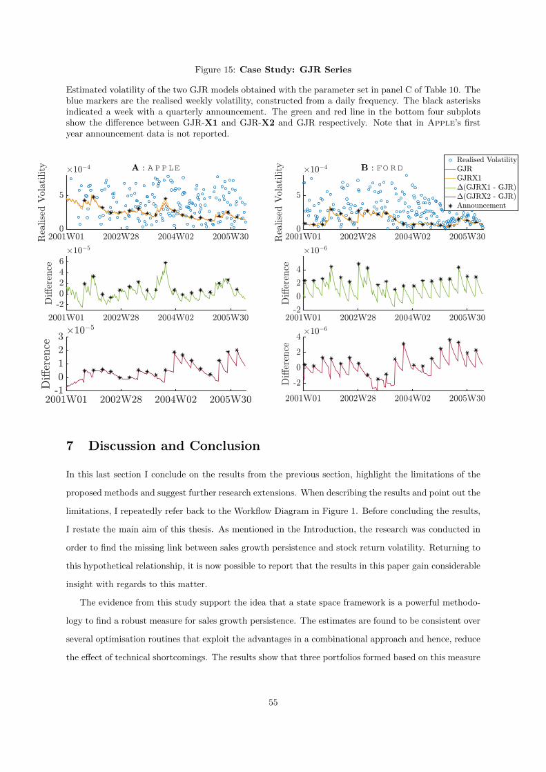
Figure 15: Case Study: GJR Series

Estimated volatility of the two GJR models obtained with the parameter set in panel C of Table 10. Theblue markers are the realised weekly volatility, constructed from a daily frequency. The black asterisksindicated a week with a quarterly announcement. The green and red line in the bottom four subplotsshow the difference between GJR-X1 and GJR-X2 and GJR respectively. Note that in Apple’s firstyear announcement data is not reported.

A PPLE FO R D

7 Discussion and Conclusion

In this last section I conclude on the results from the previous section, highlight the limitations of the

proposed methods and suggest further research extensions. When describing the results and point out the

limitations, I repeatedly refer back to the Workflow Diagram in Figure 1. Before concluding the results,

I restate the main aim of this thesis. As mentioned in the Introduction, the research was conducted in

order to find the missing link between sales growth persistence and stock return volatility. Returning to

this hypothetical relationship, it is now possible to report that the results in this paper gain considerable

insight with regards to this matter.

The evidence from this study support the idea that a state space framework is a powerful methodo-

logy to find a robust measure for sales growth persistence. The estimates are found to be consistent over

several optimisation routines that exploit the advantages in a combinational approach and hence, reduce

the effect of technical shortcomings. The results show that three portfolios formed based on this measure

55

of persistence differ in numerous ways. Of these portfolio implications, the striking difference in realised

sales growth is the most significant, showing almost a ten-fold difference between the high-growth com-

panies in the high-persistence portfolio and the high-growth firms of the non-persistent portfolio. I have

demonstrated that these comprehensive results are unaffected by time span of the growth period, data

sample period or rest upon differences of overabundance of fast growing industries along the portfolios.

Thus, this concludes that for a subset of companies sales are predictable. Growing companies sorted in

the HP portfolio are on average able to realise and annual sales growth of 1.8%. This in comparison

to the unpredictable NP portfolio in which case the annual sales growth for high-growth companies is

0.13% on average.

Following the workflow of this paper, I devised a second methodology that added sales surprises as

exogenous variables to GARCH volatility models. The findings indicate that, in two thirds of the com-

panies, news about the quarterly reports adds multiple percentages to the explanatory power of GARCH

model in a regression on the realised volatility. Adding extra information about sales surprises at these

announcement moments, results in model preferences, which are mainly unaltered by the extension of

a leverage adjusted GARCH models. In terms of confirming the hypothesis that the different portfolios

might have a different reaction to announcement news, the evidence is mixed. The parameter distribu-

tions follow a similar pattern in four out five estimates except for parameter associated with positive

forecast errors. This parameter distribution differentiates in two ways, it has heavy tails and the mean

is significantly higher compared with the other two portfolios. The higher average parameter estimate

relates high-persistence to more volatility at an announcement with positive news. On the other side,

the results of Table 7, are not convincing that there is a significant difference in news reaction along the

portfolios.

Every block, link or definition from the workflow that relates fundamentals to return volatility has

influence on the findings of this study. On one side, every component implies a limiting factor, and

so the findings must be regarded with all the assumptions taken into account, while on the other side,

all the choices made early on open many different doors to future extensions. The specific choice for

the minimal number of reporting years is such an important limitation made early on and incorporate a

strong survivorship bias. All companies that exist for more than 25 years have had a period of expanding

sales, mostly in the early years or after a large merger or acquisition. The essence is that only a particular

subset of companies is able to maintain such outperformance over a different years, and will get placed

in the high-persistence portfolio. Decreasing the minimal reporting period to 5 or ten years greatly

expands the company dimension in the data set, but the question is to what extent this increases the

parameter uncertainty around the persistence parameter. As methodology in this set up focuses on a

univariate time series approach for every unique company, it would be a valuable research project, to

56

see if these results are consistent with our findings. A reasonable hypothesis would be that companies

that persistently grow below the market average or even shrink their net sales, will face default much

sooner, and so in this study would fall out of the data sample, resulting in an upward bias towards larger

annualised growth numbers in the high-persistent portfolio.

The results of section 6.2 indicate finding growth persistence in other cash flow measures, such as

earnings, will not perfectly correlate with the sales growth persistence mainly discussed in this paper. It

might be insightful to check if similar portfolio features exist for earnings or dividends.

The fact that the high-persistence portfolio was able to outperform the market average growth so

excessively, rests partially on the assigned definition of sales growth persistence. Where the conventional

literature awards persistence to consecutive years of growth, this paper considers persistence from a more

state space point of view, a mean-reverting parameter in a local linear trend model. The choice for such

a specific definition makes a bit more challenging to directly compare our results to other studies in the

field. This could be a partial explanation of why the annual returns of the portfolios do not show a

pattern consistent with the studies of Chan et al. (2003) or Chen (2017), in which high-growth portfolios

actually underperform the low growth portfolios evaluated at returns basis. One could argue that this

proposed measure is better in capturing the ‘real’ growth, because the state space model filters the noisy

growth rates. To differentiate from the standard first differences growth-rate measure is one of the main

reasons to implement the state space framework. And so it can be concluded that perhaps the earlier

studies are to much influenced by noisy growth rates. Repeating the analysis of Chan et al. (2003) and

Chen (2017) with filtered growth rates might confirm this hypothesis.

Overall the results are clearly influenced by the portfolio formation, which is based on the estimated

persistent parameter ϕ. The lack of comparable studies make it hard to give solid explanation for this

relative arbitrary choice of portfolio breakpoints other than the preference of an equally-sized portfolios.

Mainly because the LLT model is rejected for two thirds of all the companies, it not possible split the

data set in three, five or ten equally sized portfolios as is more of a custom throughout financial literature,

except for the industry formed portfolios. Sales growth persistence can be regarded as more of a company

specific label which does not fluctuate though time and therefore makes it hard to have an exact number

of reporting firms at each specific point in time. As a robustness check I altered the breakpoints to a

more equally spaced ϕ-spectrum, with thresholds for the NP portfolio from 0 to 0.3, for the LP portfolio

from 0.3 until 0.8 and the HP portfolio from 0.8 up to 1 among several other combination, as well as the

addition of a middle-persistent (MP) portfolio between LP and HP. But after bootstrapping and hence

creating equal sized portfolios, these new sets of results did not lead to significantly different conclusions.

So I believe the results to be robust to the precise definition of the portfolio thresholds.

Apart from the different portfolio thresholds based on growth persistence, I sort the portfolios a

57

second time based on the WGS, weighted average rank of sales growth. Finding an upward structure

of over the double sort is inevitable. Other possible valuable sorts include size and value. It would be

interesting to see if a double sort with size reveals return patterns more in line with Chan et al. (2003)

and growth patterns according to Chen (2017).

Following Figure 1 to the second block, that relates growth persistence to the Expectation Hypothesis.

The extension of the GARCH framework with company specific exogenous variables proves to be a

beneficial approach. For a large group of companies increases the direct explanation with regards to the

realised volatility. It is known from previous literature that the adjusted R2 that was found, is not as low

as it might seem, and so adding multiple percentages is actually considerable. An important limitation

was the frequency of the return data on which I estimated the realised volatility. Calculating the weekly

realised volatility from daily observations, generally results in a rough estimate of the underlying variance.

This estimate is a much higher number, than when it is calculated on a smaller intraday frequency, as

shown e.g. by Andersen and Bollerslev (1998a). It is straightforward to see the main reason behind this

phenomenon. When the weekly variance is calculated from an hourly return sample it will result in much

lower variance, as the sample size is increased by its tenfold. Working with a higher data frequencies also

allows a more detailed look in the days surrounding a quarterly announcement, which could be another

future extension of this study.

As an addition to the general GARCH model, this study further adds the GJR model that includes

a leverage component. Table 1 from Hansen and Lunde (2005) gives a nice overview of the GARCH

universe and, apart from GARCH and GJR-GARCH, shows 14 other different GARCH specifications.

This demonstrates that there are countless other model specifications, not covered in this study, from

which Nelson (1991)’s EGARCH model deserves to be further investigated, because of the absence of

parameter restrictions. It is also important to mention that the evaluation of the different volatility

models is not always obvious. I choose among the different models based on the AIC and R2 of the

Mincer-Zarnowitz regression, other measures could include mean-squared error or mean-absolute error.

Although I expect the results to be generally the same.

The results of this study further indicate that adding fundamental information adds to the perform-

ance of a GARCH model.The definition of this fundamental information is very important for additional

performance. Where this study uses the forecast error from observed sales minus the Kalman predicted

sales, there are many other potential additional variables. I think the general idea should remain the

same: deviation from the market’s expectation will influence volatility. Good proxies for the market’s

expectations can be found in the I/B/E/S Database. An earnings surprise measure defined in the liter-

ature subtracts the realised EPS by the analysts’ forecast. The database also contains information about

expectation of long-term growth (LTG), a exogenous variable could include the differences between the

58

LTG expectation of two periods. Periods in which this differences are larger should be related to market’s

uncertainty about long-term perspective. As Glosten et al. (1993) find a significant dummy variable for

specific months, adding a specific dummy variables might also be noteworthy. For example, the ap-

pointment of a new CEO, starting operations in a different country or more drastically, a merger or

acquisition.

Regarding the analysis of the explanatory variables in the GARCH framework, it can be implemented

in two ways. First, there is direct implication which is applied in this study, adding the exogenous variable

to the variance equation. The second approach starts with estimation of a normal GARCH model and

uses the residuals as independent variable in regression framework that incorporates these explanatory

variables. Although this approach has been left aside in thesis, future studies should also try to evaluate

the effect with this second approach.

Given the results on the current data set, I would have expected more major differences between

the estimated parameters of the different portfolios, as were found in the first part of the study. This

belief relies heavily on the hypothesis that, the market reacts different to quarterly news announcements

of high-persistent companies in comparison to low- or non-persistent companies. One could argue that,

for a high-persistent company, the market would have a relatively good idea about what to expect at a

certain point in time, whereas for a non-persistent firm it always remains a relative big surprise. On the

other hand, a large deviation from what would be expected for such a high-persistent company might

increase the uncertainty among the market participants on how to interpret such an aberrant observation,

as a short-term, mid-term or long-term change? If the question remains, you can always wonder did we

propose the right methods? Did we use the right exogenous variables in the GARCH specification? Or

is the question simply to complex to provide us with a simple answer? Finding a solution or specified

formula that explains why asset prices are so volatile, which is applicable for every company, multiple

countries outsdie the U.S., market regime, time period and with reasonable forecasting power, might

be beyond the scope of the thesis. Nonetheless, the findings of the study represent a first step in the

direction of applying company fundamentals in explaining stock return volatility.

Acknowledgements

My special thanks goes out towards Rutger-Jan Lange for his encouragement, inspiration and guidance

over the course of this thesis. I am grateful for the quick feedback and comments of Sebastiaan Vermeulen.

I wish to thank my friends and family for their motivation and support, without whose help this work

would never have been possible. Finally, in particular I thank Mathijs Verhagen and Ferdinand Boers

for their proofreading and valuable discussions.

59

References

Andersen, T. G. and Bollerslev, T. (1998a). Answering the skeptics: Yes, standard volatility models do

provide accurate forecasts. International Economic Review, 39(4):885–905.

Andersen, T. G. and Bollerslev, T. (1998b). Deutsche mark–dollar volatility: intraday activity patterns,

macroeconomic announcements, and longer run dependencies. Journal of Finance, 53(1):219–265.

Andersen, T. G., Bollerslev, T., Diebold, F. X., and Ebens, H. (2001). The distribution of realized stock

return volatility. Journal of Financial Economics, 61(1):43–76.

Ang, A., Hodrick, R. J., Xing, Y., and Zhang, X. (2006). The cross-section of volatility and expected

returns. Journal of Finance, 61(1):259–299.

Ang, A. and Liu, J. (2004). How to discount cashflows with time-varying expected returns. Journal of

Finance, 59(6):2745–2783.

Beaver, W., Kettler, P., and Scholes, M. (1970). The association between market determined and

accounting determined risk measures. Accounting Review, 45(4):654–682.

Bernard, V. L. and Thomas, J. K. (1989). Post-earnings-announcement drift: Delayed price response or

risk premium? Journal of Accounting Research, 27:1–36.

Blasco, N., Corredor, P., and Santamaria, R. (2002). Is bad news cause of asymmetric volatility response?

a note. Applied Economics, 34(10):1227–1231.

Bollerslev, T. (1986). Generalized autoregressive conditional heteroskedasticity. Journal of Econometrics,

31(3):307–327.

Bordalo, P., Gennaioli, N., La Porta, R., and Shleifer, A. (2017). Diagnostic expectations and stock

returns. NBER Working Paper, 23863.

Bottazzi, G., Coad, A., Jacoby, N., and Secchi, A. (2011). Corporate growth and industrial dynamics:

Evidence from French manufacturing. Applied Economics, 43(1):103–116.

Callen, J. L. and Segal, D. (2004). Do accruals drive firm-level stock returns? A variance decomposition

analysis. Journal of Accounting Research, 42(3):527–560.

Campbell, J. Y. (1991). A variance decomposition for stock returns. Economic Journal, 101(405):157–

179.

Campbell, J. Y. and Ammer, J. (1993). What moves the stock and bond markets? a variance decom-

position for long-term asset returns. Journal of Finance, 48(1):3–37.

60

Campbell, J. Y. and Hentschel, L. (1992). No news is good news: An asymmetric model of changing

volatility in stock returns. Journal of Financial Economics, 31(3):281–318.

Campbell, J. Y. and Kyle, A. S. (1993). Smart money, noise trading and stock price behaviour. Review

of Economic Studies, 60(1):1–34.

Campbell, J. Y. and Shiller, R. J. (1988). Stock prices, earnings, and expected dividends. Journal of

Finance, 43(3):661–676.

Chan, L. K., Karceski, J., and Lakonishok, J. (2003). The level and persistence of growth rates. Journal

of Finance, 58(2):643–684.

Chan, L. K., Lakonishok, J., and Sougiannis, T. (2001). The stock market valuation of research and

development expenditures. Journal of Finance, 56(6):2431–2456.

Chen, H. (2017). Do cash flows of growth stocks really grow faster? Journal of Finance, 72(5):2279–2330.

Chen, H. J. (2004). Expected dividend growth rates and stock returns. University of Chicago, Working

Paper.

Chung, K. H. and Pruitt, S. W. (1994). A simple approximation of Tobin’s Q. Financial Management,

23(3):70–74.

Da, Z. and Warachka, M. (2011). The disparity between long-term and short-term forecasted earnings

growth. Journal of Financial Economics, 100(2):424–442.

Da, Z. and Warachka, M. C. (2009). Cashflow risk, systematic earnings revisions, and the cross-section

of stock returns. Journal of Financial Economics, 94(3):448–468.

Daniel, K., Hirshleifer, D., and Subrahmanyam, A. (1998). Investor psychology and security market

under-and overreactions. Journal of Finance, 53(6):1839–1885.

Davis, J. L., Fama, E. F., and French, K. R. (2000). Characteristics, covariances, and average returns:

1929 to 1997. Journal of Finance, 55(1):389–406.

De Bondt, W. F. and Thaler, R. (1985). Does the stock market overreact? Journal of Finance,

40(3):793–805.

De Jong, P. (1991). The diffuse Kalman filter. The Annals of Statistics, 19(2):1073–1083.

Dechow, P. M., Kothari, S. P., and Watts, R. L. (1998). The relation between earnings and cash flows.

Journal of Accounting and Economics, 25(2):133–168.

61

Dechow, P. M., Richardson, S. A., and Sloan, R. G. (2008). The persistence and pricing of the cash

component of earnings. Journal of Accounting Research, 46(3):537–566.

Dechow, P. M. and Sloan, R. G. (1997). Returns to contrarian investment strategies: Tests of naive

expectations hypotheses. Journal of Financial Economics, 43(1):3–27.

Dempster, A. P., Laird, N. M., and Rubin, D. B. (1977). Maximum Likelihood from incomplete data via

the EM algorithm. Journal of the Royal Statistical Society. Series B (Methodological), pages 1–38.

Durbin, J. and Koopman, S. J. (2012). Time series analysis by state space methods, volume 38. Oxford

University Press.

Engle, R. F. (1982). Autoregressive conditional heteroscedasticity with estimates of the variance of

United Kingdom inflation. Econometrica, 50(4):987–1007.

Engle, R. F. and Patton, A. J. (2001). What good is a volatility model? Quantitative Finance, 1:237–245.

Ertimur, Y., Livnat, J., and Martikainen, M. (2003). Differential market reactions to revenue and expense

surprises. Review of Accounting Studies, 8(2-3):185–211.

Fama, E. F. (1965). The behavior of stock-market prices. Journal of Business, 38(1):34–105.

Fama, E. F. and French, K. R. (1988). Permanent and temporary components of stock prices. Journal

of Political Economy, 96(2):246–273.

Fama, E. F. and French, K. R. (1992). The cross-section of expected stock returns. Journal of Finance,

47(2):427–465.

Fama, E. F. and French, K. R. (1993). Common risk factors in the returns on stocks and bonds. Journal

of Financial Economics, 33(1):3–56.

Fama, E. F. and French, K. R. (1995). Size and book-to-market factors in earnings and returns. Journal

of Finance, 50(1):131–155.

Fama, E. F. and French, K. R. (2002). The equity premium. Journal of Finance, 57(2):637–659.

Fisher, G. S., Shah, R., and Titman, S. (2016). Analyst long-term growth forecasts, accounting funda-

mentals and stock returns. Gernstein Fisher Working Paper.

French, K. R., Schwert, G. W., and Stambaugh, R. F. (1987). Expected stock returns and volatility.

Journal of Financial Economics, 19(1):3–29.

62

Glosten, L. R., Jagannathan, R., and Runkle, D. E. (1993). On the relation between the expected value

and the volatility of the nominal excess return on stocks. Journal of Finance, 48(5):1779–1801.

Hansen, P. R. and Lunde, A. (2005). A forecast comparison of volatility models: Does anything beat a

GARCH (1, 1)? Journal of Applied Econometrics, 20(7):873–889.

Harvey, A. C. (1990). Forecasting, structural time series models and the Kalman filter. Cambridge

University Press.

Hecht, P. and Vuolteenaho, T. (2005). Explaining returns with cash-flow proxies. Review of Financial

Studies, 19(1):159–194.

Jegadeesh, N. and Livnat, J. (2006). Post-earnings-announcement drift: The role of revenue surprises.

Financial Analysts Journal, 62(2):22–34.

Jegadeesh, N. and Titman, S. (1993). Returns to buying winners and selling losers: Implications for

stock market efficiency. Journal of Finance, 48(1):65–91.

Kalman, R. E. (1960). A new approach to linear filtering and prediction problems. Journal of Basic

Engineering, 82(1):35–45.

Kalman, R. E. and Bucy, R. S. (1961). New results in linear filtering and prediction theory. Journal of

Basic Engineering, 83(1):95–108.

Kiger, J. E. (1974). Volatility in quarterly accounting data. The Accounting Review, 49(1):1–7.

Kitagawa, G. and Gersch, W. (1984). A smoothness priors-state space modeling of time series with trend

and seasonality. Journal of the American Statistical Association, 79(386):378–389.

Kryzanowski, L. and Mohsni, S. (2014). Persistence and current determinants of the future earnings

growth rates of firms. European Journal of Finance, 20(2):181–200.

La Porta, R. (1996). Expectations and the cross-section of stock returns. Journal of Finance, 51(5):1715–

1742.

La Porta, R., Lakonishok, J., Shleifer, A., and Vishny, R. (1997). Good news for value stocks: Further

evidence on market efficiency. Journal of Finance, 52(2):859–874.

Lakonishok, J., Shleifer, A., and Vishny, R. W. (1994). Contrarian investment, extrapolation, and risk.

Journal of Finance, 49(5):1541–1578.

Lamont, O. (1998). Earnings and expected returns. Journal of Finance, 53(5):1563–1587.

63

Lange, R.-J. and Teulings, C. N. (2018). The option value of vacant land and the optimal timing of city

extensions. Tinbergen Institute Discussion Papers, 033(III).

Lettau, M. and Wachter, J. A. (2007). Why is long-horizon equity less risky? A duration-based explan-

ation of the value premium. Journal of Finance, 62(1):55–92.

Lettau, M. and Wachter, J. A. (2011). The term structures of equity and interest rates. Journal of

Financial Economics, 101(1):90–113.

Lev, B. and Kunitzky, S. (1974). On the association between smoothing measures and the risk of common

stocks. Accounting Review, 49(2):259–270.

Malkiel, B. G. and Fama, E. F. (1970). Efficient capital markets: A review of theory and empirical work.

Journal of Finance, 25(2):383–417.

Miller, M. H. and Modigliani, F. (1961). Dividend policy, growth, and the valuation of shares. Journal

of Business, 34(4):411–433.

Nelson, D. B. (1991). Conditional heteroskedasticity in asset returns: A new approach. Econometrica,

59(2):347–370.

Ohlson, J. A. and Juettner-Nauroth, B. E. (2005). Expected EPS and EPS growth as determinants of

value. Review of Accounting Studies, 10(2-3):349–365.

Pagan, A. R. and Schwert, G. W. (1990). Alternative models for conditional stock volatility. Journal of

Econometrics, 45(1-2):267–290.

Poterba, J. M. and Summers, L. H. (1988). Mean reversion in stock prices: Evidence and implications.

Journal of Financial Economics, 22(1):27–59.

Richardson, S. A., Sloan, R. G., Soliman, M. T., and Tuna, I. (2005). Accrual reliability, earnings

persistence and stock prices. Journal of Accounting and Economics, 39(3):437–485.

Sadka, G. (2007). Understanding stock price volatility: The role of earnings. Journal of Accounting

Research, 45(1):199–228.

Sharma, J. L., Mougoue, M., and Kamath, R. (1996). Heteroscedasticity in stock market indicator return

data: Volume versus GARCH effects. Applied Financial Economics, 6(4):337–342.

Shiller, R. J. (1981). Do stock prices move too much to be justified by subsequent changes in dividends?

The American Economic Review, 71(3):421–436.

64

Shumway, R. H. and Stoffer, D. S. (1982). An approach to time series smoothing and forecasting using

the EM algorithm. Journal of Time Series Analysis, 3(4):253–264.

Sloan, A. (1996). Do stock prices fully reflect information in accruals and cash flows about future

earnings? Accounting Review, 71(3):289–315.

Stock, J. H. and Watson, M. W. (1998). Median unbiased estimation of coefficient variance in a time-

varying parameter model. Journal of the American Statistical Association, 93(441):349–358.

Summers, L. H. (1986). Does the stock market rationally reflect fundamental values? Journal of Finance,

41(3):591–601.

Van Binsbergen, J., Brandt, M., and Koijen, R. (2012). On the timing and pricing of dividends. American

Economic Review, 102(4):1596–1618.

Vuolteenaho, T. (2002). What drives firm-level stock returns? Journal of Finance, 57(1):233–264.

Watson, M. W. and Engle, R. F. (1983). Alternative algorithms for the estimation of dynamic factor,

mimic and varying coefficient regression models. Journal of Econometrics, 23(3):385–400.

65

A Appendix A: Proofs and Derivations

A.1 Derivation of the Kalman Filter and Smoother

The derivation of the Kalman filter and smoother are based on the three Lemma’s of the (joint) normal

distribution.

Lemma 1 When X and Y are independent normally distributed random variables, their sum is also

normally distributed:

N(µX ,ΣX) + N(µY ,ΣY ) ∼ N(µX + µY ,ΣX + ΣY ).

Lemma 2 Pre-multiplying a normal random variable with a non-stochastic matrix C:

C ·N(µ,Σ) ∼ N(Cµ,CΣC ′).

Lemma 3 Suppose X and Y are jointly normally distributed random variables with:

X

Y

∼ N

µX

µY

,

ΣXX ΣXY

Σ′XY ΣY Y

.

Then the conditional distribution of X given Y is normal with mean and variance:

E[X|Y ] = µX + ΣXY Σ−1Y Y (Y − µY ),

Var(X|Y ) = ΣXX − ΣXY Σ−1Y Y Σ′XY .(A.1)

Note: Even if X and Y are not normally distributed, equation A.1 is still the Minimum Variance Linear

Unbiased Estimator (MVLUE), with corresponding variance matrix Var(X|Y )

To derive the formulas in the Kalman algorithm, let αt be the optimal estimator of the state vector

αt conditional of all information up to, and including observation yt, also referred to as and P is the

corresponding covariance matrix of the estimation error. Then by means of the joint normal distribution,

αt|It ∼ N(αt|t,Pt|t), where

αt|t = E[αt|It],

Pt|t = Var(αt|It) = E[(αt − αt)(αt − αt)′|It].(A.2)

66

When we recall the state equation, from equation 1 and combine it with Lemma 1 and 2, we obtain the

distribution of αt+1|It and the best possible prediction for the next time point t+ 1,

αt+1|It ∼ N(T αt|t +Φct,TPt|tT +RQR′), (A.3)

αt+1|It ∼ N(αt+1|t,Pt+1|t),

with the corresponding prediction equations,

αt+1|t = T αt|t +Φct,

Pt+1|t = TPt|tT′ +RQR′.

(A.4)

Once the best predictions are known, the optimal forecast of yt+1 given It is,

E[yt+1|It] = Z ′αt+1|t +Ωdt (A.5)

the corresponding one-step ahead prediction error vt+1|t and prediction error variance Ft+1|t,

vt+1|t = yt+1 −Z ′αt+1|t −Ωdt,

Ft|t = Z ′Pt+1|tZ +H.

(A.6)

The covariance between the prediction error vt+1|t and the estimated state αt+1|t is,

Cov(αt+1, vt+1|It) = Cov(αt+1, yt+1 −Z ′αt+1|t −Ωdt)

= Cov(αt+1,Z′αt+1 +Ωdt + εt+1 −Z ′αt+1|t −Ωdt) = Z ′Pt+1|t

When a new observation becomes available, the best estimate can be updated. From the joint distribution

of both αt+1, yt+1 conditional on the information at t, It,

yt+1

αt+1

It ∼ N

Z ′αt+1|t +Ωdt

αt+1|t

,

Z ′Pt+1|tZ +H Z ′Pt+1|t

Pt+1|tZ Pt+1|t

, (A.7)

using equation A.1 from Lemma 3 it follows that the new distribution of αt+1|yt+1, It is,

αt+1|yt+1, It ∼ N(αt+1|t+1,Pt+1|t+1), (A.8)

67

where both αt+1|t+1 and Pt+1|t+1 follow from the updating equation 5, where vt|t is the one-step ahead

forecast error and Ft|t its corresponding forecast error matrix.

αt+1|t+1 = αt+1|t + Pt+1|t +ZF−1t|t vt|t

Pt+1|t+1 = Pt+1|t − Pt+1|tZF−1t|t Z

′Pt+1|t

(A.9)

Once the Kalman Filter reaches the end of the series, it is possible to derive a conditional density of

αt given all the observations. The smoother iterates backwards through the sample and updates the

predicted estimates, based on all available information IT , this specific type of smoother is known as

the classical fixed-interval smoother. The smoothed state vector αt follows a normal distribution with

expected state αt|T and state variance Pt|T defined as,

αt|T = E[αt|IT ] Pt|T = Var(αt|IT ). (A.10)

Following from the tower property, we can rewrite the expected state vector to,

αt|T = E[αt|IT ] = Eαt+1[E[αt|αt+1, IT ]|IT ]. (A.11)

The inner expectation of the above relation, can again be rewritten to E[αt|αt+1, IT ] = E[αt|αt+1, It],

because we know that the information in αt+1 contains all the relevant information that is needed for αt.

Again using equation A.1 from Lemma 3 the joint conditional distribution of αt and αt1 on information

set It becomes, αt

αt+1

It ∼ N

αt|t

αt+1|t

,

Pt|t Pt|tT ′

TPt|t Pt+1|t

(A.12)

where the covariance term is the result of the inner product of the expectation of αt and αt+1,

Cov((αt,αt+1|It)) = Cov(αt,Tαt +Φct +Rηt) = Pt|tT′.

Focusing on the conditional expectation of αt given both αt+1 and the complete information set IT ,

with the result of joint distribution A.12 and the tower property (αt+1|T = E[αt+1|IT ]),

E[αt|αt+1, IT ] = αt|t + Pt|tT′P−1t+1|t(αt+1 − αt+1|t)

αt|T = Eαt+1 [αt|t + Pt|tT′P−1t+1|t(αt+1 − αt+1|t)]|IT ]

αt|T = αt|t + Pt|tT′P−1t+1|t(αt+1|T − αt+1|t).

(A.13)

.

68

The derivation of the state variance follows the same line of thought,

Pt|T = Var(αt|IT ) = E[(αt − αt|T )(αt − αt|T )′|IT ]

= E[αtα′t|IT ]− αt|T α′t|T ,

(A.14)

but requires an expression for the last term, E[αtα′t|IT ], which by means of the tower property in

equation A.11 results in,

E[αtα′t|IT ] = Eαt+1

[E[αtα′t|αt+1, It]|IT ], (A.15)

the inner expectation in the above, is a bit less straightforward, but ends up with two terms,

E[αtα′t|αt+1, It] = E[αt|αt+1, It]E[αt|αt+1, It]′ + Var(αt|αt+1, It)

= E[αt|αt+1, It]E[αt|αt+1, It]′ + Pt|t − Pt|tT ′P−1t+1|tTPt|t

= [αt|t + Pt|tT′P−1t+1|t(αt+1 − αt+1|t)]

2 + Pt|t − Pt|tT ′P−1t+1|tTPt|t,

(A.16)

using these two terms in the original equation A.15,

E[αtα′t|IT ] = Eαt+1

[E[αtα′t|αt+1, It]|IT ]

= Eαt+1[[αt|t + Pt|tT

′P−1t+1|t(αt+1 − αt+1|t)]2]

+ Eαt+1 [Pt|t − Pt|tT ′P−1t+1|tTPt|t]

= αt|T α′t|T + Eαt+1 [Pt|tT

′P−1t+1|t(αt+1 −αt+1|T )(αt+1 −αt+1|T )′P−1t+1|tTPt|t]

+ Pt|t − Pt|tT ′P−1t+1|tTPt|t

E[αtα′t|IT ]− αt|T α′t|T = Pt|tT

′P−1t+1|tPt+1|T P−1t+1|tTPt|t + Pt|t − Pt|tT ′P−1t+1|tTPt|t

= Pt|t + Pt|tT′P−1t+1|t(Pt+1|T − Pt+1|t)P

−1t+1|tTPt|t

(A.17)

together, equation A.13, A.14 and A.17 result in the Kalman smoothing equations,

αt|T = αt|t + Pt|tT′P−1t+1|t(αt+1|T − αt+1|t)

Pt|T = Pt|t − Pt|tT ′P−1t+1|t(Pt+1|t − Pt+1|T )P−1t+1|tT′Pt|t

(A.18)

69

A.2 Derivation of the EM Algorithm

The derivation of the formulas evaluated in the EM algorithm start with the joint log-likelihood of a

general state space model from data y1, ..., yT and states α0, ...,αT

`(y1, ..., yT ,α0, ...,αT |θ) =− 1

2log(|Σ0|)−

1

2(α0 − µ0)′Σ−10 (α0 − µ0)

− 1

2

T∑

t=1

log(|H−1|)− (yt −Zαt −Ωdt)′H−1(yt −Zαt −Ωdt)

+ log(|Q−1|)− (αt − Tαt−1 −Φct)′Q−1(αt − Tαt−1 −Φct).

(A.19)

Note the addition of two row vectors, Φ and Ω which are associated with time varying constant column

vectors ct and dt. In the first step we take the conditional expectation over this joint log-likelihood for

a given parameter set conditional on all the data,

E[`(y1, ..., yT ,α0, ...,αT |θ, IT )], (A.20)

and in the second step we maximise over all the parameters θ, such that,

∂

∂θE[`(y1, ..., yT ,α0, ...,αT |θ, IT )] = 0. (A.21)

The parameter set θ basically contains all system matrices and vectors, and hence all are prompt to

a specific partial derivative. Assume for a moment that for a certain parameter set and all informa-

tion on the data, the expectation of the log-likelihood, E[`(y1, ..., yT ,α0, ...,αT |θ, IT ) resolves into just

`(y1, ..., yT ,α0, ...,αT ), or simply abbreviated to `. To derive all the partial derivatives of ` with re-

spect to the system vectors, matrices we start with H and Q the observation and state variance terms

respectively,

∂`

∂H−1=T2H − 1

2

T∑

t=1

(yt −Z ′αt −Ωdt)(yt −Z ′αt|t −Ωdt)′ = 0,

H =1

TT∑

t=1

(yt −Z ′αt −Ωdt)(yt −Z ′αt −Ωdt)′,(A.22)

∂`

∂Q−1=T2Q− 1

2

T∑

t=1

(αt − Tαt−1 −Φct)(αt − Tαt−1 −Φct)′ = 0,

Q =1

TT∑

t=1

(αt − Tαt−1 −Φct)(αt − Tαt−1 −Φct)′.(A.23)

70

The transition matrices Z and T require rules of differentiating matrices with use traces.

∂`

∂Z ′= −1

2

∂

∂Z ′Tr

[H−1

∑Tt=1(yt −Z ′αt −Ωdt)(yt −Z ′αt −Ωdt)′spaceshipsssi

]= 0,

= −1

2

∂

∂Z ′Tr

H−1∑Tt=1(yty

′t −Z ′αty′t − ytα′tZ +Z ′αtα′tZ + ...

spa− ytd′tΩ′ −Ωdty′t +Ωdtα′tZ +Z ′αtd′tΩ

′ +Ωdtd′tΩ′)

= 0,

= −1

2

T∑

t=1

(−(αty′tH−1)′ − (H−1ytα′t) + (αtα

′tZH

−1)′ + ...

spa+ (H−1Z ′αtα′t) + (αtd′tΩ′H−1)′ + (H−1Ωdtα′t)spaceee

= 0,

= H−1T∑

t=1

[ytα

′t −Z ′αtα′t +Ωdtα

′tspaceeeeeeeeeeeeeeeeeeeeeeeeeeeeeeei

]= 0,

Z ′ =

(∑Tt=1 ytα

′t +Ωdtα

′t

)(∑Tt=1αtα

′t

)−1,

(A.24)

∂`

∂T= −1

2

∂

∂TTr

[Q−1

∑Tt=1(αt − Tαt−1 −Φct)(αt − Tαt−1 −Φct)′spaceeeeeeeeew

]= 0,

= −1

2

∂

∂TTr

Q−1∑nt=1(αtα

′t −αtα′t−1T ′ − Tαt−1α′t + Tαt−1α′t−1T

′ + ...i

spa −Φctα′t −αtc′tΦ′ + Tαt−1c′tΦ′ +Φctα′t−1T ′ +Φctc′tΦ′)

= 0,

= −1

2

T∑

t=1

(−Q−1αtα′t−1 −αt−1α′tQ−1 + (αt−1α′t−1T′Q−1)′ + ...

+Q−1Tαt−1α′t−1 +Q−1αtc′tΦ′ +Φctα′t−1Q

−1spaceeeeeeeeeeeeee

= 0,

= Q−1T∑

t=1

[αtα

′t−1 − Tαt−1α′t−1 +Φctα

′t−1spaceeeeeeeeeeeeeeeeeeeeeeeeeeee

]= 0,

T =

(∑Tt=1αtα

′t−1 +Φctα

′t−1

)(∑Tt=1αt−1α

′t−1

)−1.

(A.25)

The last two derivations are for the system matrices, Ω and Φ,

∂`

∂Ω= −1

2

∂

∂ΩTr

[H−1

∑Tt=1(yt −Z ′αt −Ωdt)(yt −Z ′αt −Ωdt)′spaceshipeee

]= 0,

= −1

2

∂

∂ΦTr

H−1∑Tt=1(yty

′t −Z ′αty′t − ytα′tZ +Z ′αtα′tZ + ...

spa− ytd′tΩ′ −Ωdty′t +Ωdtα′tZ +Z ′αtd′tΩ

′ +Ωdtd′tΩ′)

= 0,

= −1

2

T∑

t=1

−H−1dty′t − ytd′tH−1 +Z ′αtdtH−1 +H−1dtα′tZ + ...space

+dtd′tΩ′H−1 +H−1Ωdtdt

= 0,

= H−1T∑

t=1

[−ytd′t +Z ′αtd′t +Ωdtd

′tspaceeeeeeeeeeeeeeeeeeeeeeeeeeeeeee

]= 0,

Ω =

(∑Tt=1−ytd′t +Z ′αtd′t

)(∑Tt=1 dtd

′t

)−1,

(A.26)

71

∂`

∂Φ= −1

2

∂

∂ΦTr

[Q−1

∑Tt=1(αt − Tαt−1 −Φct)(αt − Tαt−1 −Φct)′spaceshipeeee

]= 0,

= −1

2

∂

∂ΦTr

Q−1∑Tt=1(αtα

′t −αtα′t−1T ′ − Tαt−1α′t + Tαt−1α′t−1T

′ + ...

spa−Φctα′t −αtc′tΦ′ + Tαt−1c′tΦ′ +Φctα′t−1T ′ +Φctc′tΦ′)spa

= 0,

= −1

2

T∑

t=1

−Q−1αtc′t − ctα′tQ−1 + Tαt−1c′tQ

−1 +Q−1ctα′t−1T′ + ...space

+ctc′tΦ′Q−1 +Q−1Φctc′t

= 0,

= Q−1T∑

t=1

[−αtc′t + Tαt−1c′t +Φctc

′tspaceeeeeeeeeeeeeeeeeeeeeeeeeeeeeeeei

]= 0,

Φ =

(∑Tt=1−αtc′t + Tαt−1c′t

)(∑Tt=1 ctc

′t

)−1.

(A.27)

For the sake of simplicity, I have made an assumption about the expectation of the log-likelihood resulting

in the six equations above. When we now explicitly calculate the conditional expectation, equation A.22

until equation A.27 can be easily altered. The output of the Kalman smoothing equations, provide

the expression for the conditional expectation of αt given the complete information set, E[αt|IT ] =

αt|T , E[αtα′t|IT ] = αt|T α′t|T + Pt|T and E[αtα

′t−1|IT ] = αt|T α′t−1|T + Pt,t−1|T , where Pt,t−1|T is the

covariance between αt and αt−1, this results in,

H = E[

1T∑Tt=1

(yt −Z ′αt −Ωdt

)(yt −Z ′αt −Ωdt

)′IT],

= E

1T∑Tt=1

yty′t − ytα′tZ − ytd′tΩ′ −Z ′αty′t −Z ′αtα′tZ + ...

+Z ′αtd′tΩ′ −Ωdty′t +Ωdtα

′tZ +Ωdtd

′tΩ′

IT

,

=1

TT∑

t=1

yty′t − ytα′t|T Z − ytd′tΩ′ −Z ′αt|T y′t −Z ′[αt|T α′t|T + Pt|T ]Z + ...

+Z ′αt|T d′tΩ′ −Ωdty′t +Ωdtα

′t|T Z +Ωdtd

′tΩ′

(A.28)

Q = E[

1T∑Tt=1

(αt − Tαt−1 −Φct

)(αt − Tαt−1 −Φct

)′IT],

= E

1T∑Tt=1

αtα′t −αtα′t−1T ′ −αtc′tΦ′ − Tαt−1α′t + Tαt−1α′t−1T

′ + ...

+Tαt−1c′tΦ′ −Φctα′t +Φctαt−1T ′ +Φctc′tΦ

′

IT

,

=1

TT∑

t=1

[αt|T α′t|T + Pt|T ]− [αt|T α′t−1|T + Pt,t−1|T ]T ′ − αt|T c′tΦ′ + ...

−T [αt−1|T α′t|T + Pt,t−1|T ] + T [αt−1|T α′t−1|T + Pt−1|T ]T ′ + ...

+T αt−1|T c′tΦ′ −Φctα′t|T +Φctαt−1|T T ′ +Φctc′tΦ

′

, (A.29)

72

Z ′ = E[(∑Tt=1 ytα

′t +Ωdtα

′t

)(∑Tt=1αtα

′t

)−1IT],

=

(∑Tt=1 ytα

′t|T +Ωdtα

′t|T

)(∑Tt=1 αt|T α

′t|T + Pt|T

)−1, (A.30)

T = E[(∑Tt=1αtα

′t−1 +Φctα

′t−1

)(∑Tt=1αt−1α

′t−1

)−1IT],

=

(∑Tt=1 αt|T α

′t−1|T + Pt,t−1|T +Φctα

′t−1|T

)(∑Tt=1 αt−1|T α

′t−1|T + Pt−1|T

)−1, (A.31)

Ω = E[(∑Tt=1−ytd′t +Z ′αtd′t

)(∑Tt=1 dtd

′t

)−1IT],

=

(∑Tt=1−ytd′t +Z ′αt|T d′t

)(∑Tt=1 dtd

′t

)−1, (A.32)

Φ = E[(∑Tt=1−αtc′t + Tαt−1c′t

)(∑Tt=1 ctc

′t

)−1IT],

=

(∑Tt=1−αt|T c′t + T αt−1|T c′t

)(∑Tt=1 ctc

′t

)−1. (A.33)

In the latter four system matrices, the last term in a matrix inverse. If the dimensions of the problem

increase, and if not all states are connected resulting in many empty off diagonal elements, computation

of these matrix inverses gets problematic. To provide stable numerical results it is often replaced by the

Moore-Penrose inverse or matrix pseudoinverse.

The log-likelihood function also depends on the prior state α0, which is assumed to be normally

distributed, α0 ∼ N

(µ0,Σ0

), and therefore the same first order conditions apply as to the other

system matrices. Differentiating the log-likelihood function with respect to µ0 and Σ0 yield,

µ0 = α0, Σ−10 =

(α0 − µ0

)(α0 − µ0

)′. (A.34)

Taking the expectation conditional on the complete data set results in the best estimates for the prior

states,

E[µ0 IT

]= α0|T E

[Σ0 IT

]= E

[(α0 − α0

)(α0 − α0

)′]= P0|T . (A.35)

73

A.3 Optimising Initial Values

It starts with the variance of the first differences, for a univariate local level model,

Var(∆yt) = Var(yt − yt−1) = Var(ηt + εt − εt−1) = σ2η + 2 σ2

ε ,

if both σ2ε and σ2

η are in the same order, it is useful to set the initialisation to,

σ2η =

1

2Var(yt − yt−1), σ2

ε =1

4Var(yt − yt−1).

For the local linear mean-reverting trend model, the trend δt has the similar structure as an AR(1)

process, for which it known that the variance in steady state is given by,

Var(δt) = ϕ2 Var(δt−1) + σ2ζ =

σ2ζ

1− ϕ2.

Using the above, the variance of the first differences becomes,

Var(∆yt) = Var(yt − yt−1) = Var(δt−1 + ηt + εt − εt−1) =σ2ζ

1− ϕ2+ σ2

η + 2 σ2ε .

If again σ2ε , σ2

η and σ2ζ are of equal magnitude a proper starting value is,

σ2ε =

1

6Var(yt − yt−1), σ2

η =1

3Var(yt − yt−1), σ2

ζ = (1− ϕ2)1

3Var(yt − yt−1).

To find a decent starting value for the ϕ without using the Kalman filter, I examine the auto-covariance

structure of the trend, following from the AR(1) structure,

Cov(δt, δt−n) =1

1− ϕ2ϕn σ2

ζ .

The auto-covariance structure of the first differences,

E[(yt+1 − yt)(yt − yt−1)] = Cov(δt, δt−1) + E[−ε2t ] =1

1− ϕ2ϕ σ2

ζ − σ2ε

E[(yt+1 − yt)(yt−n − yt−n−1)] = Cov(δt, δt−n−1) =1

1− ϕ2ϕn σ2

ζ , for n > 0.

We find that Cov(yt+1−yt)(yt−n−yt−n−1) declines exponentially with the rate ϕ. Therefore the natural

logarithm of this covariance, log(Cov(yt+1 − yt)(yt−n − yt−n−1)), should be somewhat linear and log(ϕ)

74

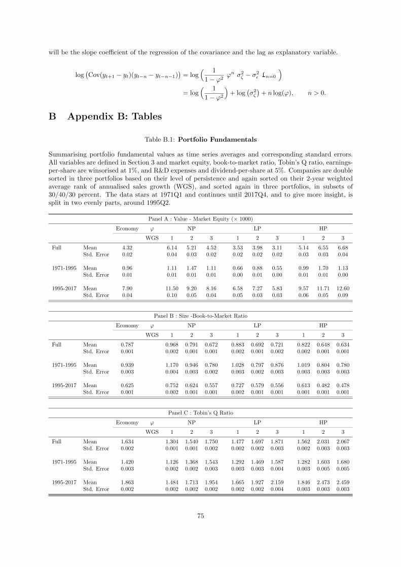
will be the slope coefficient of the regression of the covariance and the lag as explanatory variable.

log(Cov(yt+1 − yt)(yt−n − yt−n−1)

)= log

( 1

1− ϕ2ϕn σ2

ζ − σ2ε 1n=0

)

= log( 1

1− ϕ2

)+ log

(σ2ζ

)+ n log(ϕ), n > 0.

B Appendix B: Tables

Table B.1: Portfolio Fundamentals

Summarising portfolio fundamental values as time series averages and corresponding standard errors.All variables are defined in Section 3 and market equity, book-to-market ratio, Tobin’s Q ratio, earnings-per-share are winsorised at 1%, and R&D expenses and dividend-per-share at 5%. Companies are doublesorted in three portfolios based on their level of persistence and again sorted on their 2-year weightedaverage rank of annualised sales growth (WGS), and sorted again in three portfolios, in subsets of30/40/30 percent. The data stars at 1971Q1 and continues until 2017Q4, and to give more insight, issplit in two evenly parts, around 1995Q2.

Panel A : Value - Market Equity (× 1000)

Economy ϕ NP LP HP

WGS 1 2 3 1 2 3 1 2 3

Full Mean 4.32 6.14 5.21 4.52 3.53 3.98 3.11 5.14 6.55 6.68Std. Error 0.02 0.04 0.03 0.02 0.02 0.02 0.02 0.03 0.03 0.04

1971-1995 Mean 0.96 1.11 1.47 1.11 0.66 0.88 0.55 0.99 1.70 1.13Std. Error 0.01 0.01 0.01 0.01 0.00 0.01 0.00 0.01 0.01 0.00

1995-2017 Mean 7.90 11.50 9.20 8.16 6.58 7.27 5.83 9.57 11.71 12.60Std. Error 0.04 0.10 0.05 0.04 0.05 0.03 0.03 0.06 0.05 0.09

Panel B : Size -Book-to-Market Ratio

Economy ϕ NP LP HP

WGS 1 2 3 1 2 3 1 2 3

Full Mean 0.787 0.968 0.791 0.672 0.883 0.692 0.721 0.822 0.648 0.634Std. Error 0.001 0.002 0.001 0.001 0.002 0.001 0.002 0.002 0.001 0.001

1971-1995 Mean 0.939 1.170 0.946 0.780 1.028 0.797 0.876 1.019 0.804 0.780Std. Error 0.003 0.004 0.003 0.002 0.003 0.002 0.003 0.003 0.003 0.003

1995-2017 Mean 0.625 0.752 0.624 0.557 0.727 0.579 0.556 0.613 0.482 0.478Std. Error 0.001 0.002 0.001 0.001 0.002 0.001 0.001 0.001 0.001 0.001

Panel C : Tobin’s Q Ratio

Economy ϕ NP LP HP

WGS 1 2 3 1 2 3 1 2 3

Full Mean 1.634 1.304 1.540 1.750 1.477 1.697 1.871 1.562 2.031 2.067Std. Error 0.002 0.001 0.001 0.002 0.002 0.002 0.003 0.002 0.003 0.003

1971-1995 Mean 1.420 1.126 1.368 1.543 1.292 1.469 1.587 1.282 1.603 1.680Std. Error 0.003 0.002 0.002 0.003 0.003 0.003 0.004 0.003 0.005 0.005

1995-2017 Mean 1.863 1.484 1.713 1.954 1.665 1.927 2.159 1.846 2.473 2.459Std. Error 0.002 0.002 0.002 0.002 0.002 0.002 0.004 0.003 0.003 0.003

75

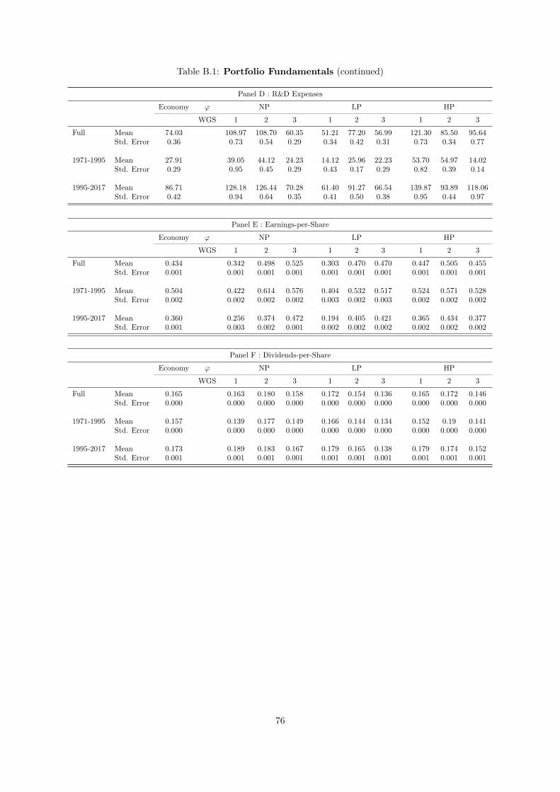
Table B.1: Portfolio Fundamentals (continued)

Panel D : R&D Expenses

Economy ϕ NP LP HP

WGS 1 2 3 1 2 3 1 2 3

Full Mean 74.03 108.97 108.70 60.35 51.21 77.20 56.99 121.30 85.50 95.64Std. Error 0.36 0.73 0.54 0.29 0.34 0.42 0.31 0.73 0.34 0.77

1971-1995 Mean 27.91 39.05 44.12 24.23 14.12 25.96 22.23 53.70 54.97 14.02Std. Error 0.29 0.95 0.45 0.29 0.43 0.17 0.29 0.82 0.39 0.14

1995-2017 Mean 86.71 128.18 126.44 70.28 61.40 91.27 66.54 139.87 93.89 118.06Std. Error 0.42 0.94 0.64 0.35 0.41 0.50 0.38 0.95 0.44 0.97

Panel E : Earnings-per-Share

Economy ϕ NP LP HP

WGS 1 2 3 1 2 3 1 2 3

Full Mean 0.434 0.342 0.498 0.525 0.303 0.470 0.470 0.447 0.505 0.455Std. Error 0.001 0.001 0.001 0.001 0.001 0.001 0.001 0.001 0.001 0.001

1971-1995 Mean 0.504 0.422 0.614 0.576 0.404 0.532 0.517 0.524 0.571 0.528Std. Error 0.002 0.002 0.002 0.002 0.003 0.002 0.003 0.002 0.002 0.002

1995-2017 Mean 0.360 0.256 0.374 0.472 0.194 0.405 0.421 0.365 0.434 0.377Std. Error 0.001 0.003 0.002 0.001 0.002 0.002 0.002 0.002 0.002 0.002

Panel F : Dividends-per-Share

Economy ϕ NP LP HP

WGS 1 2 3 1 2 3 1 2 3

Full Mean 0.165 0.163 0.180 0.158 0.172 0.154 0.136 0.165 0.172 0.146Std. Error 0.000 0.000 0.000 0.000 0.000 0.000 0.000 0.000 0.000 0.000

1971-1995 Mean 0.157 0.139 0.177 0.149 0.166 0.144 0.134 0.152 0.19 0.141Std. Error 0.000 0.000 0.000 0.000 0.000 0.000 0.000 0.000 0.000 0.000

1995-2017 Mean 0.173 0.189 0.183 0.167 0.179 0.165 0.138 0.179 0.174 0.152Std. Error 0.001 0.001 0.001 0.001 0.001 0.001 0.001 0.001 0.001 0.001

76

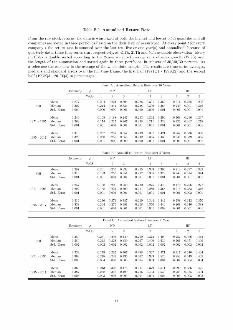
Table B.2: Annualised Return Rate

From the raw stock returns, the data is winsorized at both the highest and lowest 0.5% quantiles and allcompanies are sorted in three portfolios based on the their level of persistence. At every point t for everycompany i the return rate is summed over the last ten, five or one year(s) and annualised, because ofquarterly data, these time series start respectively, at 41Th, 21Th and 5Th available observation. Everyportfolio is double sorted according to the 2-year weighted average rank of sales growth (WGS) overthe length of the summation and sorted again in three portfolios, in subsets of 30/40/30 percent. Asa reference the economy is the average of the whole data sample. The results are time series averages,medians and standard errors over the full time frame, the first half (1971Q1 - 1995Q2) and the secondhalf (1995Q3 - 2017Q4) in percentages.

Panel A : Annualised Return Rate over 10 Years

Economy ϕ NP LP HP

WGS 1 2 3 1 2 3 1 2 3

Full

Mean 0.277 0.204 0.224 0.304 0.226 0.301 0.362 0.211 0.278 0.298Median 0.302 0.214 0.241 0.334 0.238 0.300 0.365 0.240 0.301 0.316Std. Error 0.000 0.000 0.000 0.001 0.000 0.000 0.001 0.001 0.001 0.001

1971 - 1995Mean 0.243 0.168 0.188 0.247 0.213 0.262 0.299 0.168 0.216 0.237Median 0.263 0.174 0.215 0.267 0.228 0.271 0.323 0.226 0.262 0.278Std. Error 0.001 0.001 0.001 0.001 0.001 0.001 0.001 0.001 0.001 0.001

1995 - 2017

Mean 0.313 0.237 0.257 0.357 0.239 0.337 0.421 0.252 0.336 0.356Median 0.325 0.238 0.255 0.356 0.242 0.355 0.430 0.246 0.339 0.365Std. Error 0.001 0.001 0.000 0.000 0.000 0.001 0.001 0.000 0.001 0.001

Panel B : Annualised Return Rate over 5 Years

Economy ϕ NP LP HP

WGS 1 2 3 1 2 3 1 2 3

Full

Mean 0.287 0.201 0.235 0.332 0.215 0.309 0.393 0.216 0.297 0.322Median 0.310 0.193 0.255 0.351 0.217 0.305 0.378 0.240 0.314 0.344Std. Error 0.001 0.001 0.001 0.001 0.001 0.001 0.001 0.001 0.001 0.001

1971 - 1995Mean 0.257 0.168 0.200 0.280 0.220 0.275 0.348 0.176 0.256 0.277Median 0.292 0.168 0.221 0.300 0.211 0.280 0.368 0.216 0.283 0.316Std. Error 0.001 0.001 0.001 0.001 0.001 0.001 0.001 0.001 0.002 0.001

1995 - 2017

Mean 0.319 0.236 0.271 0.387 0.210 0.344 0.442 0.258 0.342 0.370Median 0.338 0.264 0.275 0.391 0.218 0.350 0.446 0.261 0.346 0.388Std. Error 0.001 0.001 0.001 0.001 0.001 0.001 0.002 0.001 0.001 0.001

Panel C : Annualised Return Rate over 1 Year

Economy ϕ NP LP HP

WGS 1 2 3 1 2 3 1 2 3

Full

Mean 0.350 0.231 0.293 0.440 0.259 0.373 0.490 0.252 0.366 0.412Median 0.380 0.248 0.323 0.450 0.267 0.400 0.530 0.261 0.371 0.409Std. Error 0.002 0.002 0.002 0.002 0.002 0.002 0.002 0.002 0.002 0.002

1971 - 1995Mean 0.339 0.219 0.265 0.407 0.298 0.367 0.471 0.217 0.346 0.404Median 0.368 0.248 0.282 0.435 0.302 0.389 0.526 0.252 0.349 0.409Std. Error 0.003 0.004 0.003 0.003 0.004 0.003 0.004 0.004 0.004 0.004

1995 - 2017

Mean 0.362 0.243 0.322 0.476 0.217 0.379 0.511 0.290 0.386 0.421Median 0.387 0.258 0.356 0.499 0.216 0.403 0.539 0.285 0.375 0.404Std. Error 0.003 0.003 0.003 0.003 0.004 0.004 0.004 0.003 0.003 0.003

77