thesis.eur.nl · Web viewThe impact of government policies and international trade on Indian...
89
The impact of government policies and international trade on Indian agriculture ERASMUS UNIVERSITY ROTTERDAM Erasmus School of Economics Department of Economics Supervisor: Dr. Koen Berden 1
Transcript of thesis.eur.nl · Web viewThe impact of government policies and international trade on Indian...

The impact of government policies and
international trade on Indian agriculture
ERASMUS UNIVERSITY ROTTERDAM
Erasmus School of Economics
Department of Economics
Supervisor: Dr. Koen Berden
Name: Rohan Girish Gujar
Exam number: 314979
E-mail address: [email protected]
1

Acknowledgements
An academic work is by its very nature a continuation on earlier work and as such builds on the foundation laid
down by earlier scholars. This thesis is no different. The credit for this naturally goes to my supervisor Dr. Koen
Berden. It would not have been possible for me to complete this task without his invaluable guidance for which I am
extremely grateful.
I would also wish to thank Mr. Ashish Panda for providing valuable guidance in developing this thesis. Finally I also
wish to express my gratitude to my parents for providing me this opportunity.
Rohan Gujar
26th of August 2013
2

Abstract
The recent rise in suicide rates amongst farmers in India today is the symptom of an underlying crisis in agriculture
due to the marginalization of the agrarian economy. It may partially be explained as a result of an increasingly
globalized environment and the presence of supranational economic regimes such as the WTO and The World Bank
which to a certain extent influences the government policy on agriculture, particularly those regarding subsidies
given to farmers, international trade tariffs as well as non-tariff measures. The policies of the Government of India
too, are not helpful to the farmer as the twin objectives of the government to keep food prices under control on one
hand and to ensure fair prices to the farmer on the other hand are often conflicting and result in unpredictable trade
policies. This results in restraining the farmers from selling their produce in the international markets whenever
convenient as well as instituting tariff and other barriers for agricultural imports.
In this research, we have used the Global Simulation Model (GSIM) for partial equilibrium analysis of two crucial
crops produced in India. Further I have also computed the welfare gains for three separate scenarios, namely; (a) an
ambitious scenario, (b) a very ambitious scenario, and (c) a limited scenario. The ambitious scenario is a free trade
agreement between India and EU where the bilateral tariff is completely abolished. The very ambitious scenario is
also a free trade agreement but it is assumed that EU will also abolish its export subsidies to India . The limited
scenario is a less ambitious version of the ambitious one in terms of depth of the liberalization. The research finds
that free trade in the said commodities does result in positive producer and consumer surplus but also to dropping
prices for cotton and wheat produce. The net welfare effects for scenario one, two and three for cotton for India are
130.5, 126.6 and 59.6 million USD respectively. The welfare effects for wheat are 11.1, 15.6 and 7.2 million USD
for scenario one, two and three respectively. However, the prices for cotton drop by a maximum of 2.3% only, while
wheat prices may decrease by up to 13% - seriously affected incomes of Indian farmers. If these price decreases are
not compensated for by increases in production and exports onto the world markets, Indian wheat farmers may lose
out, aggravating the worries of the Indian government of further marginalization of certain agricultural sectors An
EU-India FTA is not the same as a multilateral free trade approach and the Indian government may want to analyze
carefully comparative advantages of trade partners before engaging in bilateral trade talks. Moreover, this research
shows clearly that EU CAP reform affects the way the Indian farmers are affected – the less subsidized the EU
farmers the lower the cotton and wheat imports from the EU and the less prices for produce drop – leaving Indian
farmers with higher world prices for cotton and wheat.
The research concludes by recommending fewer restraints for the farmer and promoting a more liberal free trade
policy in agricultural products.
Key Words: Agriculture, International Trade Policy, Subsidy, WTO, GSIM Model and India.
3
4

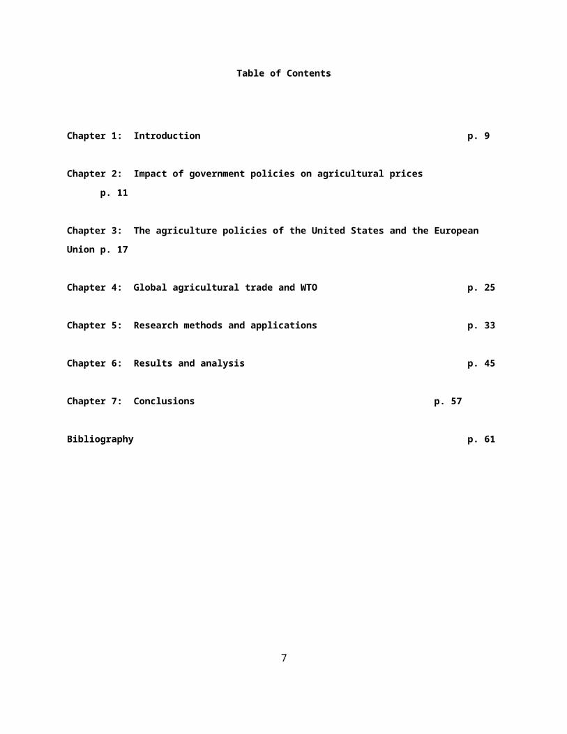
Table of Contents
Chapter 1: Introduction p. 9
Chapter 2: Impact of government policies on agricultural prices p. 11
Chapter 3: The agriculture policies of the United States and the European Union p. 17
Chapter 4: Global agricultural trade and WTO p. 25
Chapter 5: Research methods and applications p. 33
Chapter 6: Results and analysis p. 45
Chapter 7: Conclusions p. 57
Bibliography p. 61
5

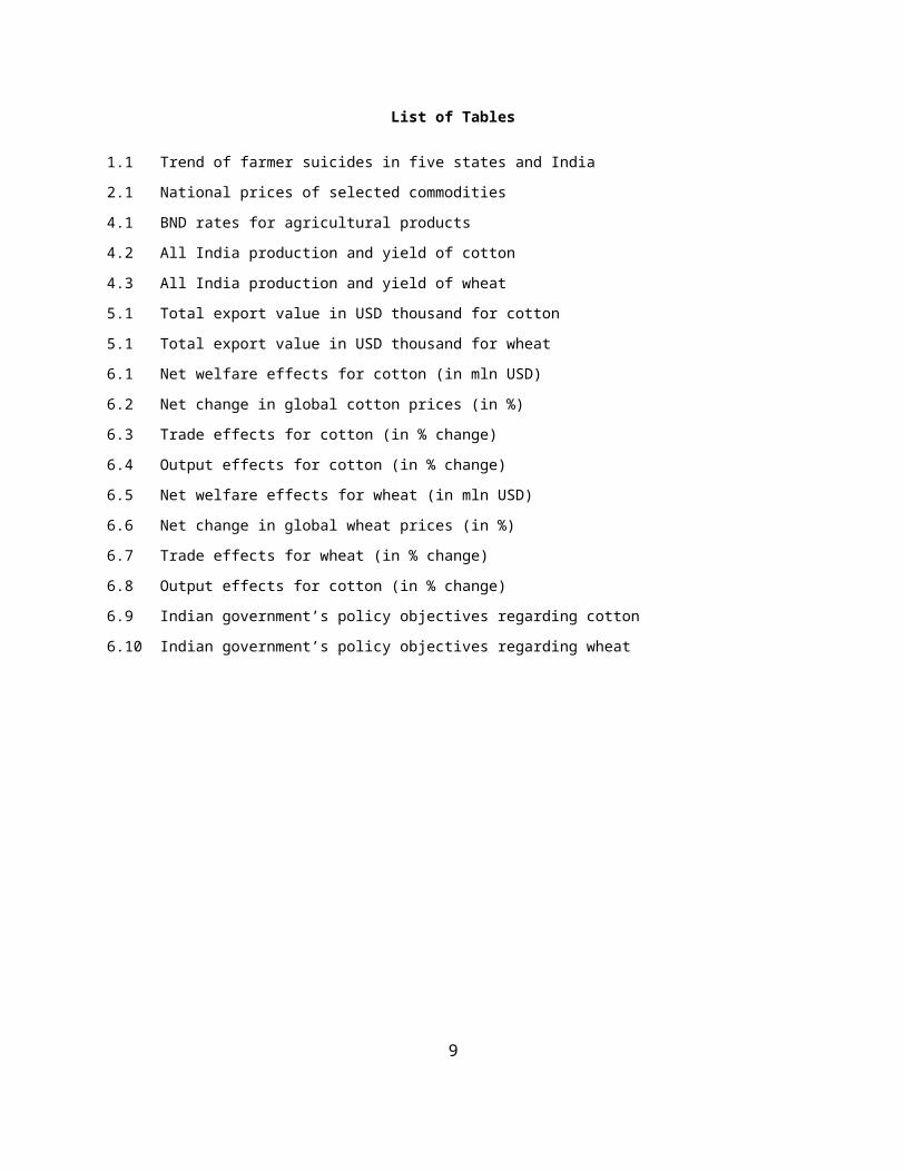
List of Tables
1.1 Trend of farmer suicides in five states and India
2.1 National prices of selected commodities
4.1 BND rates for agricultural products
4.2 All India production and yield of cotton
4.3 All India production and yield of wheat
5.1 Total export value in USD thousand for cotton
5.1 Total export value in USD thousand for wheat
6.1 Net welfare effects for cotton (in mln USD)
6.2 Net change in global cotton prices (in %)
6.3 Trade effects for cotton (in % change)
6.4 Output effects for cotton (in % change)
6.5 Net welfare effects for wheat (in mln USD)
6.6 Net change in global wheat prices (in %)
6.7 Trade effects for wheat (in % change)
6.8 Output effects for cotton (in % change)
6.9 Indian government’s policy objectives regarding cotton
6.10 Indian government’s policy objectives regarding wheat
6
List of Figures
2.1 Top production – India – 2011
2.2 Top production – Wheat – 2011
3.1 World cotton production
3.2 World wheat production
7

Chapter 1
Introduction
“There is something terribly wrong in the countryside” (Swaminathan, 2006). This was stated in the context of a
sharp rise in the number of suicides among Indian farmers. These events are constantly reported in India. Between
1995 and 2011 there have been over 250,000 farmer suicides in India. High debt levels were found to be the most
common cause. An in depth analysis reveals that indebtedness is a symptom (Posani, 2006). The increasing number
of suicides was an indication of distress in Indian agriculture as a whole. Indeed there has been a distinct slowdown
in agricultural growth over the past two decades (Gill.et.al, 2006). Obsolete technology, increased cost prices and
declining profitability have all made cultivation a non-profitable enterprise, thereby threatening the livelihood of
farmers, particularly the small and marginal ones
Table 1.1: Number of farmer suicides in five states and India in total
Year Maharashtra Andhra Pradesh
Karnataka Madhya Pradesh
&Chhattisgarh
Total of 5 states
All India
1997 1917 1097 1832 2390 7236 136221998 2409 1813 1883 2278 8333 160151999 2423 1974 2379 2654 9430 160822000 3022 1525 2630 2660 9837 166032001 3536 1509 2505 2824 10374 164152002 3695 1896 2340 2578 10509 179712003 3836 1800 2678 2511 10825 171642004 4147 2666 1963 3033 11809 182412005 3926 2490 1883 2660 10959 171312006 4453 2607 1720 2858 11638 170602007 4238 1797 2135 2856 11026 166322008 3802 2105 1737 3152 10797 16196Total 41404 23279 25685 32454 122823 199132Average 3450 1940 2140 2704 10235 16594
Source: www.indiatogether.org
However, couple of decades ago this scenario would have been unimaginable. The “father of green revelation” and
then then Minister of Agriculture Dr. C. Subramanian, formed the “New Agricultural Strategy” in the early 60’s,
marking the beginning of the agricultural revolution and strengthening of the farmer’s lobby (Das, 2007). The
miracle technologies of the “Green Revolution” aided by massive input subsidies provided by the government led to
big leap in agricultural production. This resulted in the ever increasing demand by farmers for additional subsidies
and output prices. “Farmer Power” grew so strong that their demands could not be ignored.
9
Most developed countries use a combination of domestic market interventions by way of minimum support prices
and various direct and indirect subsidies to protect the interests of their farmers who thus derive a competitive
advantage which could be and is argued as unfair by numerous scholars (Mishra, 2007).
It is obvious that the agrarian interests that were once upon a time dominant, have become marginalized. This leads
us to the main research question:
To what extent do the national, international and supra-national agriculture policies impact the welfare,
output and trade of and market price for produce obtained by the Indian farmer– with a specific focus on
analyzing the impact of the EU-India Free Trade Agreement on the cotton and wheat sectors.
In order to answer the research question, we look at the following research elements: What are the main national,
international and supra-national agriculture policies? How do these policies affect the market prices of agriculture
products? How can this question best be quantitatively analyzed? What are the reliable sources of data? To what
extent the inferences drawn be applicable to other agri-products? What are the policy recommendations?
Will a policy change lead to reduction in farmer suicides? In the next chapter we expound upon the main national
agriculture policies and their impact on Indian farmer followed by a chapter on international agriculture policies
particularly those of the United States and European Union and their impact on Indian agriculture. The fourth
chapter discusses the role of a supra-national institution such as World Trade Organization (WTO) in the context of
global agricultural trade while chapter five talks about how best the research question be quantitatively analyzed
with a focus on EU-India trade. Chapter six displays the results while the last chapter draws inferences and makes
policy recommendations.
10

Chapter 2
Impact of Indian government policies on agricultural prices
In this chapter, we first begin with a brief history of Indian agriculture in section 2.1. This is followed by the impact
of government policy on agricultural prices in briefly discussed in section 2.2. Declining productivity, changing crop
production patterns and rising cost of cultivation and declining state support is discussed in sections 2.3, 2.4 and 2.5.
Section 2.6 discusses declining irrigation. Finally, in section 2.7 and 2.8 price shocks and credit squeeze are
discussed.
2.1. A brief history of Indian agriculture
Prima-facie it appears that the Indian farmer’s demands for enhanced prices are in conflict against economic
constraints such as a plateauing of technology, a demand constraint from India’s poor if food prices are kept high,
and the fiscal limits of increasing subsidization (Joshi, 1998). (Furthermore, it also appears the market reforms of the
1990s and the subsequent shift in economic priorities of the Indian government initially did help in improving
productivity of this sector to a great extent but were not followed up by the next stage of reforms such as allowing
foreign direct investment in retail, insurance and infrastructure which directly led to stagnation of agriculture and
subsequent hardships for the farmers (Menon, 2004).
This paradigm shift was also partially related to the changing global political environment which increasingly
curtailed the availability of policy space for national governments (Bhagwati, 2007). Fundamentally this is because
there are inherent limits for the growth of a purely agricultural economy (Sen, 2004).
It is well-known that Indian agriculture was in dire straits in 1947. Prior to that due to several reasons including the
two world wars the agricultural growth was a mere 12 % whereas the population grew by 40% resulting in a decline
in per capita food availability.
As such there was no alternative but to increase agriculture production for which the farmer had to be provided with
incentives. There were two approaches available. The first approach of increasing the food prices, investing in
hybrid seeds, fertilizers and irrigation as well as giving subsidies to the farmers was unaffordable as the government
was committed to keeping the food prices low and hence the second “cheaper” institutional approach was opted for
to increase productivity. This approach had two steps: institution of land reforms to provide incentives to the actual
tiller as compared to the land owner to produce more along with the creation of farm and service cooperatives to
avail benefits of economies of scale. These cooperatives were created and controlled by politicians in power (even
today) especially in the agriculturally rich states of Maharashtra, Punjab, Karnataka, Andhra Pradesh and Haryana.
Due to heavy monsoons in the 50’s, there was development in irrigation and expansion of acreage but not yield.
Production soon became stagnant due to the poor monsoons for two years in a row during 1965 and 1966, and the
11

country was pushed to the brink of famine and as a result large quantities of grains had to be imported at discounted
rates from US, Canada and Australia.
Hence the late 60s saw a shift in India’s agricultural policy by providing price incentives and making large
investments in irrigation, chemical fertilizers and technology to increase yields. Two new institutions: The
Agricultural Prices Commission (APC) and The Food Corporation of India (FCI), were set up during this period
which assisted the growth process. The FCI made price recommendations favorable to producers which resulted in
increased food grain production and increased area under high yield variety seeds by 1970-71. Thus, a ‘Green
Revolution’ was born.
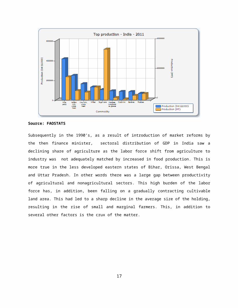
Figure 2.1: Top production – India - 2011
Source: FAOSTATS
Subsequently in the 1990’s, as a result of introduction of market reforms by the then finance minister, sectoral
distribution of GDP in India saw a declining share of agriculture as the labor force shift from agriculture to industry
was not adequately matched by increased in food production. This is more true in the less developed eastern states
of Bihar, Orissa, West Bengal and Uttar Pradesh. In other words there was a large gap between productivity of
agricultural and nonagricultural sectors. This high burden of the labor force has, in addition, been falling on a
gradually contracting cultivable land area. This had led to a sharp decline in the average size of the holding,
resulting in the rise of small and marginal farmers. This, in addition to several other factors is the crux of the matter.
12

Figure 2.2: Top production – Wheat – 2011
Source: FAOSTATS
2.2 Impact of government policies on agricultural prices
Indian Policy makers face the enormous challenge of adjusting domestic agriculture policies, with the objective to
stabilize food prices. Encouraging agricultural trade, through reduction of tariff and non-tariff barriers has been
widely recommended as critical in successfully resolving this conundrum. According to the Food & Agriculture
ministry, usually, domestic food production at any given time is sufficient to meet local requirement, as such
facilitating freer movement of grains would certainly help in meeting isolated shortfalls. Swaminathan (2006) has
also argued that “free trade in the region would facilitate large-scale production of food grains with comparative
advantage, and improve regional food security, even in drought period”. An effective reply mechanism to stop
emergencies as suggested by the WTO is simplification of trade regulations (WTO, 2011).
Despite these policy recommendations and the numerous researches undertaken by well-known scholars, there is
insufficient understanding of the precise impacts of specific trade policies on farmers. This has forced the
government to keep India significantly closed where trade in agricultural commodities is concerned. The objective
to isolate and protect food markets in the country is not totally unreasonable, considering that most of the population
is still poor and lives without adequate nutrition. In the absence of sufficient purchasing power they are also
susceptible to minor shifts in supply or prices. It has therefore also been argued that openness may exacerbate
vulnerability to external shocks and threaten food security (Arlindo and Tschirley, 2003).
It is a fact in development economics that the process of development of a country involves a transformation of the
economy whereby there is a shift in terms of the value of output as well as employment from agriculture to
13

manufacturing and services sectors. It is thus reasonable to expect agriculture to decline in India and witness a
transfer of resources from this sector to the service sector.
All of this in the absence of sufficient tax revenues indicates larger budget deficit and inflation which we are indeed
witnessing today. It is a catch 22 situation.
2.3 Declining productivity in agriculture
In the last two decades, India has witnessed population growth, particularly amongst the poor and uneducated
people. This has been more so in the less developed states of Uttar Pradesh, Bihar, Orissa, Jharkhand and
Chhattisgarh. These are also to a large extent non-industrialized states and hence more dependent on agriculture. As
a direct consequence of this phenomenon, the burden of this labor force has been falling and between 1960 and
2009, the number of holdings only doubled from 51 million to 101 million, while the area cultivated declined from
133 million hectares to 108 million hectares. This has also resulted in the reduction of the average size of the
holding, and thus there has been an increase in the number of small and marginal farmers. This leads to increasing
costs, inadequate returns and accessing credit (Assadi, 1998).
Farmers in India are divided into categories depending on their land holding size. First, marginal farmers holding
less than1 hectare, second, small-sized farmers that hold one to two hectares, third, are semi-medium-sized farmers
who have two to four hectares, fourth medium-sized farmers four to ten hectares, and lastly, large-sized farmers who
hold more than ten hectares.
Productivity here refers to the crop output which is measured in yield/hectares. The increase in population as well
as the GDP necessitates greater supply of agricultural product in order to meet the increasing demand and to keep
prices stable. Thus agricultural farm land productivity is a critical parameter for the economy.
The relationship between the size of farms and agricultural produce in India, has given the economists a lot to argue
over. According to Sen (2004), increase in the number of farm holdings result in productivity decline and price rise.
On the other hand, when the prices received by the farmers for their crops are compared with the prices they pay for
consumer goods it is observed that farmers are facing erosion of real incomes (Mishra, 2007). This has resulted in
declining relative living standards of farmers as well as their ability to bear risks. As such a slight increase in risk
can destroy them.
2.4 Changing crop production patterns
When the Indian economy opened up in the 1990s, the farmers moved from the subsistence crops to the cash crops
as they were hopeful of export opportunities and higher world prices for agricultural commodities (Menon, 2004).
Devaluation of the rupee made Indian exports cheaper and hence attractive on the world market, and further helped
lead this charge into cash crops (Christian Aid, 2005). On aggregate, the total area of the country’s farmland
14

growing traditional grains declined by 18% in the decade after 1990-91, whereas areas growing non-food crops of
cotton and sugarcane increased by 25% and 10% respectively (Shiva, 2005).
2.5 Rising cost of cultivation and declining state support
Cash crops, particularly the High Yield Variety (HYVs)are input heavy. They require much greater amounts of
water, fertilizers and pesticides to grow and to yield the promised output. However, the state subsidies on these
inputs have declined over the last decade (Posani, 2006). This led to farmers having to depend increasingly on the
market for their inputs, leading to an increased cost of cultivation. Increased cost of seeds is in part due to large
amounts of foreign seeds which now flood the market for example the price of the controversial BT cotton is 4 times
higher than the domestic hybrid varieties of seeds (Asadi, 1998). The productivity of this seed might be enhanced
but the price received is not commensurate with the increased risk. It is thus not surprising to note that the maximum
number of suicides have been those of cotton farmers.
2.6 Declining irrigation
Despite a shift in cropping patterns towards more water intensive cash crops, the aggregate net irrigated area has
remained stagnant. Successive state governments have been unable to invest in surface irrigation infrastructure
(Chandrasekhar and Ghosh, 2004). Groun-water usage has led to the need for deeper and deeper wells, electric
motors and other techniques that were not readily available to subsistence farmers, pushing them into debt problems
causing higher rates of suicide.
2.7 Price shocks
Apart from such output losses, price shocks have also caused greater uncertainty to the farmers. Agricultural trade
was liberalized gradually with India’s accession to WTO. By 2000, all Quantitative Restrictions (QR) on agricultural
products were removed and brought under the tariff system.
Table 2.1: National Prices of Selected Commodities
Year Cotton (USD/100kg) Wheat (USD/100kg)
2000 240.55 13.36
2001 281.52 12.86
2002 292.59 14.71
in 305.86 17.05
2004 290.90 17.76
2005 316.71 20.12
2006 326.34 24.69
2007 426.32 26.12
15

Year Cotton (USD/100kg) Wheat (USD/100kg)
2008 538.04 23.54
2009 539.64 29.78
2010 721.40 28.57
2011 639.90 23.23
Source: Ministry of Statistics and Program Implementation, Government of India
This led to a sudden surge in cheap agricultural imports thus substantially depressing prices of agricultural
commodities. It is worth repeating here that most of the politicians have a strong agricultural constituency as well as
vested interests in the sector. It also has a, perhaps unintended consequence of bankrupting some of the local
farmers. Import duty on cotton, for instance, was almost zero, leading to a sharp fall in the price of cotton; the
benefits of which were availed by the textile industry. Farmers now find themselves vulnerable to the vicissitudes of
world prices where fluctuations are rife in addition to the risks they face due to natural calamities which makes their
propositions even riskier especially in the absence of affordable crop insurance. This combination of yield shock and
price shock that occurs simultaneously adds a new element of risk to farming (Suri and Rao, 2006).
2.8 Credit squeeze
The withdrawal of the state from providing institutional credit support was perhaps most acutely felt by the farmers
and with agriculture becoming more costly the farmers had no choice but to look for external sources of credit.
The nationalization of the banks in 1969 required them to increase lending to agriculture, with tight interest-rate
controls. But this came to an abrupt end in 1990s. The public sector banks slowly squeezed credit lines to farmers as
the sectoral risks increased and more profitable opportunities beckoned.
The farmers were left with no choice but to depend on ‘informal’ sources for credit that came with a very high rate
of interest (anything between 36% and 100% compound). This hold of the -moneylender is the main cause for
exploitation and misery. Credit from these agents is usually in terms of inputs such as seeds and fertilizers) issued
against the future output (Suri, 2006).
“The drying up of institutional credit and exploitative informal credit traps in the face of rising costs and declining
profitability have led to pervasive indebtedness among farmers. A tragic manifestation of this has been the
phenomenon of suicides among desperate farmers.” (Sainath, 2005)
16
Chapter 3
The agriculture policies of the United States and the European Union
3.1 The Common Agriculture Policy (CAP) of the European Union
The OECD secretariat has stated that in 2009 support for agricultural producers just in OECD member countries
totaled $292 billion on average per year between 2006 and 2008 (OECD, 2009a). As a result of this the competition
is distorted by high protection granted to domestic producers in agriculture, by granting subsidies in agriculture
(World Bank, 2008).Various Studies by (Hertel and Winters, 2005) have investigated the extent to which such
distortions have affected the developing country exports
Farmers in EU have been encouraged to produce crops by a combination of market price support export subsidies
and direct payments, For instance; the total production support for wheat alone averaged about $10 billion annually
during 2006-2008, corresponding to a protection rate of almost 50 percent. Since the cost of producing wheat is very
high in EU, so to compensate farmers for reduction in intervention price, direct payments are given to farmers under
various schemes, and they are encouraged to continue growing wheat even at a higher cost of production. Thus the
total subsidy works out to be in excess of 50%.This wheat is then dumped into the world market at a price which is
much lower than the domestic cost of production in those countries. This has adversely affected the farmers of
developing nations.
The share of agriculture in GDP in the EU has been declining since 1960s. It has fallen from 4.4% in 1980 to 1.7%
in 2008. On the other hand agriculture has more importance in developing economies such as India where it
constitutes 26% of the national GDP. The employment factor also tells a similar story where more than 50% of the
population is engaged in agricultural activities compared to less than 5% of the EU. However the total direct and
indirect subsidies given for agriculture are in excess of 50% thus rendering the agricultural produce of the
developing countries uncompetitive.
17

Figure 3.1: World cotton production
Figure 3.2: World wheat production 2010
22%
17%
16%
9%
6%
6%
5%
4%
3%3%
3%
1% 1% 1% 1% 1% 0%
ChinaIndiaUSARussiaAustraliaCanadaPakistanTurkeyArgentinaKazakhastanIranMoroccoBrazilUkraineAlgeriaMexicoTunisia
Source: http://www.nationmaster.com/red/pie/agr_gra_whe_pro-agriculture-grains-wheat-production
18

The Common Agricultural Policy (CAP) was initially implemented with an objective to increase agricultural
productivity in the EU. However it now aims to protect agriculture in the EU by controlling prices and quantities
produced. It does so by providing subsidies and assuring minimum support prices for farm products. The CAP also
tries to control production by setting limits on the quantities that a farmer can produce by paying the farmers not to
produce more. It has become controversial because it is seen as an unfair way of protecting European agriculture
3.2 Policy background
The CAP was created in 1957 under the Treaty of Rome and started operating in 1962. Despite attempts to reform it
no significant reduction in the level of subsidies paid to farmers has been effected. Since 2005 farmers are no longer
subsidized, but are paid a single farm payment and are expected to produce crops that are in demand by the
consumers and in that way they become the paid guardians of the countryside.
The CAP is a form of protectionism designed to protect European farmers from cheaper products outside the EU.
This was once done by subsidizing agricultural produce but similar results are now achieved by deterring imports by
using a system of import tariffs and simultaneously subsidizing farmers through the Single Farm Payment. When the
produce of the farmers is bountiful the EU subsidizes exports of the same at less than cost price or will store it and
later sell it to the under developed countries like Africa. The CAP also tries to control production by setting limits on
the quantities that a farmer can produce then paying them not to produce more.
According to the EU the reasoning behind the CAP is that the EU is compelled to look after its farmers because they
help protect the countryside and secondly because the free market is unstable and if the EU did not intervene prices
would fluctuate and farmers would not be able to respond to consumer demand. But this argument could be used by
others too. The EU should be aware that resources are best allocated through a free market: CAP thus makes food
more expensive in the EU than it need be. The CAP is thereby playing a role in increasing poverty in poor countries
by promoting unhealthy competition with local farmers. Thirdly the CAP makes a very high contribution to support
only a small minority of farmers.
In May 2008 a major review of the CAP was conducted by the commission to try to make it more efficient. Its main
proposals were: reducing SFPs to large farms and increasing the amount of funds transferred to the Rural
Development budget. Other proposals included subsidizing farmers who grow crops for bio-fuels and abolishing the
'set aside' scheme that paid farmers to leave a part of their land unfarmed so that they do not produce more.
3.2 Policy Background
The CAP was created in 1957 under the Treaty of Rome. Despite attempts to reform it no significant reduction in
the level of subsidies paid to farmers has been effected. Since 2005 farmers are no longer subsidized, but are paid a
single farm payment and are expected to produce crops that are in demand by the consumers and in that way they
19

become the paid guardians of the countryside. When the produce of the farmers is bountiful the EU subsidizes
exports of the same at less than cost price or will store it and later sell it to the under developed countries like Africa.
According to the EU the reasoning behind the CAP is that the EU is compelled to look after its farmers because they
help protect the countryside and secondly because the free market is unstable and if the EU did not intervene prices
would fluctuate and farmers would not be able to respond to consumer demand. But this argument could be used by
others too. The CAP is thereby playing a role in increasing poverty in poor countries by promoting unhealthy
competition with local farmers. Finally the CAP is beneficial for a small minority of farmers only.
3.3 Effect of CAP
The EU plays a major role in international agricultural trade; As a result of the CAP the agricultural prices paid by
EU consumers are much higher than those prevailing in international markets. The removal of the CAP would
benefit the EU households handsomely both as taxpayers and consumers. It is obvious that removal of the CAP may
reduce the number of people employed in the agricultural sector, but it would also generate substantial benefits for
the consumers and other sectors by way of lower prices for agricultural products. Other countries would also benefit
from increased demand for their exports and a healthy competition in their own markets. Trade would increase,
providing a modest benefit for growth in the EU and elsewhere.
3.4 Common Agriculture Policy and Sustainability
The European countryside It has been shaped by farming over the centuries. Farming has created the diverse
environment and its varied landscapes and provides the habitat for a great diversity of fauna and flora. The farmers
manage the countryside for the benefit of all and as such supply public goods – the most important of which is the
good care and maintenance of soils, landscapes and biodiversity. As the market does not pay for these public goods
the European Commission thought it to be fair and reasonable to compensate the farmers for this service to society
as a whole, by providing with income support. Considering that the farmers could also be adversely affected by
climate change hence the CAP provides them with financial assistance to adjust their farming methods and systems
to cope with the effects of a changing climate. To avoid negative side-effects of some farming practices, the EU
provides incentives to farmers to work in a sustainable and environmentally-friendly manner. In effect, farmers have
a double challenge: to produce food whilst simultaneously protecting nature and safeguarding biodiversity.
Income support payments from the CAP are increasingly used by farmers to adopt environmentally sustainable
farming methods. This enables them, for example, to reduce the amount of chemical fertilizer or pesticide that they
apply to their crops. Other adaptations include leaving field boundaries uncultivated, creating ponds or other
landscape features and planting trees and hedges. These are aspects of farming which go beyond what are usually
considered to be conventional farming methods and good farming practices. In addition, the CAP promotes
agricultural practices such as maintaining permanent grassland and safeguarding the scenic value of the landscape.
Protecting biodiversity and wildlife habitats, managing water resources and dealing with climate change are other
priorities that farmers are required to respect. 20

As much as 50% of the population of the EU lives in rural areas. Without farming there would be little to hold them
together. If farming were to disappear, in many areas there would be a problem of land abandonment. This is why
the CAP gives farmers financial assistance to ensure that they continue working the land and to create additional
jobs through landscape preservation or cultural heritage projects and many other tasks directly or indirectly
associated with farming and the rural economy. Many farmers are old and are expected to retire from active farming
in the near future. The EU recognizes that the age structure of farmers has become a matter of concern. Helping
young farmers get started is a policy ‘must’ if Europe’s rural areas are successfully to meet the many challenges that
face them.1 The CAP also helps farmers to be more productive and to improve their technical skills. In the face of
the food surpluses which resulted due to enhanced productivity, the emphasis has changed to: reduction of emissions
of greenhouse gases, use eco-friendly farming techniques, meet public health, environmental and animal welfare
standards, make more productive use of forests and woodland, and develop new uses for farm products in sectors
like cosmetics, medicine and handicrafts.
3.5 Common Agriculture Policy and Quality Standards
The CAP also provides labeling and logos that guarantee the authenticity of traditional foods. Over 1 000 foods
carry an EU quality logo. People can buy local and traditional foods, confident that the description on the packaging
is true. Foods must satisfy certain minimum quality standards. Uniform standards for particular goods allow
consumers to compare prices from different producers (Thomson,2009). Organic production methods must comply
with strict EU legislation. Organic farming respects the natural life cycles of plants and livestock. In the EU, organic
food is identified by a special logo (McVittie, A., Moran, D. and Thomson, S., 2009).
The CAP encourages certification systems that guarantee environmental and animal welfare conditions under which
foods have been produced. EU rules are applied from the farm to the table. Imported products must meet the same
standards as foods produced by EU farmers. The purpose of these standards is to maintain food safety levels as
products pass along the food chain.
The European Union is the world’s biggest importer of foodstuffs – by a big margin. Through its overseas
development policy, the EU helps developing countries to sell their agricultural products in the EU. It does this by
granting preferential access to its market. Each year, the EU typically imports close to €60 billion worth of
agricultural products from developing countries. The EU has extensive commercial and cooperation links with third
countries and regional trading blocs. However the cost of ensuring higher quality standards is quite high by way of
usage of expensive inputs and also due to conduction of quality control checks and quality audits. Such quality
standards can in effect act as entry barriers, thus rendering the agricultural products from developing country
uncompetitive.
1 A partnership between Europe and farmers: http://europa.eu/pol/agr/flipbook/en/files/agriculture.pdf 21

3.6 US agricultural policy
The agricultural policy was designed to stabilize and boost farm income through the provision of price and income
support for a specific list of commodities, to aid economic recovery and development during the Depression and
post-war eras. This was achieved through a combination of taxpayer-funded production payments and supply
management, in the form of acreage limits and commodity storage programs. Since then, agricultural policies have
been amended to address additional objectives. For example, beginning with the 1985, 1990 and 1996 Farm Acts,
the United States undertook major initiatives in domestic agricultural policy reform, including the elimination of
deficiency payments and the introduction of Production Flexibility Contracts (PFC) under the 1996 Farm Act. It
culminated in the ending of the supply management commodity programs.
On average, US support levels to producers are relatively moderate in comparison with average levels in other
OECD countries. Overall, although US support levels for agriculture have varied widely over time and across
commodities, the evolution of the Producer Support Estimate (PSE) and related support indicators clearly indicate a
substantial decrease.
A feature of US support levels is that they move inversely with world commodity prices. The prices have peaked
twice once in 1986-87 and the second in 1998 to 2000. Both events occurred at times when world commodity prices
were depressed in terms of US dollars. Support levels subsequently declined somewhat and then fell to relatively
low levels, when world prices rose rapidly. However, the price increase was temporary. The level of market
protection provided to producers, as measured by the Producer Nominal Protection Coefficient (PNPC), also
decreased over time and is much lower than the corresponding average PNPC in the OECD area. While in 1986-88
prices received by US farmers were 13% higher than world prices, in 2007-09 they were only 2% higher.
3.7 Impact of OECD agricultural policies on India
With changes in OECD's agricultural policies and if domestic subsidies are eliminated and tariff levels are relaxed
there could be a decline in the production in the OECD countries, which will naturally help the world prices to rise
from a depressed level. This will result in a boost in production in developing countries like India and bring about a
change in the welfare of farmers in this country. The impact will be felt differently for different crops and regions
but is unlikely to be negative. It will harm the OECD farmer much less (which can be compensated in different
ways) and benefit not only the farmers but also the consumers.
Apart from subsidizing their agricultural produce the policies of OECD countries also impact the prices of processed
foods and animal products such as milk, pork and beef. As India is neither a major consumer nor producer of these
products it is fairly unaffected by such policies. But developed countries such as China, Japan and South Korea are
affected by them as it adversely affects their domestic markets. Hence there is a strong reaction from their citizenry
who insist that their domestic producers be equally subsidized failing which the imports of such items be banned.
22
India, however happens to be a major producer of animal feed crops such as soya, groundnut and oilcake which is
exported in large quantities to numerous countries particularly to Russia and Eastern Europe. The trade in such crops
is highly subsidized by the government but does not face much opposition globally as no other producer is adversely
affected. However it should also be noted that India is one of the largest producer and consumer of milk, which is
also highly subsidized, but does not export it abroad and hence does not face any opposition. Ironically the fact that
such subsidies also prevent imports of milk products from Europe is largely ignored.
23

Chapter 4
Global Agricultural Trade and WTO
4.1 Background
The study of the economics of international trade in agriculture and food products has been an area of specialization
in the agricultural economics profession for quite some time (Giordani et. al., 2012). The main areas that dominated
the research are production economics, marketing and policy, each of which acknowledged the existence of
international trade. This chapter aims to document the role of the World Trade Organization (WTO) by identifying
some of the major contributions of the institution to international trade in agriculture.
The WTO is the only organization in the world that supervises the international trade between nations. The WTO
provides a framework to negotiate and formalize trade agreements aimed at reducing trade obstacles. It also provides
a legal framework for the implementation of these agreements together with any trade disputes arising from their
interpretation and application.
4.2 General Agreements on Tariffs and Trade (GATT)
The GATT was established during the UN Conference on Trade and Employment. On account of the failure of the
negotiating governments to create the International Trade Organization (ITO) in the aftermath of the second world
war the GAAT was formed. GATT was a set of rules for the free conduct of international trade agreed upon by the
nations involved. The GATT was signed in 1947 and lasted until 1993.There were a total of eight rounds. Given the
complexity of the issues and the need for extensive policy compromise, GATT negotiations have often been lengthy.
The Tokyo round lasted for 7 years (1973-1979), also in part due to the oil crises. The GAAT was updated in 1993,
to include new obligations, one of the most significant being creation of the World Trade Organization. The original
75 members of the GATT and the European Communities became the founding members of the WTO.
4.3 Framework and functions of the WTO
The WTO is responsible for the implementation, administration and operation of the covered agreements. Also, it is
a forum for negotiations and for settling disputes. The regulations and rules of WTO could broadly be divided under
several heads. To begin with we have the Non Discrimination Function which has two sub divisions namely the
Most Favored Nation (MFN) and the National Treatment Policy (NTO). These regulations cover trade in goods,
services and intellectual property. The next function covers Reciprocity rules which reflect a desire to limit the
scope of abuse of granting of MFN status It also indicates a desire to obtain better access to foreign markets. The
Binding and enforcing commitments encompass the tariff commitments made by the members of the WTO in a
multi-lateral trade negotiation and are enumerated in a list of concessions. These are the “ceiling bindings” which: a
country cannot change unilaterally. The Transparency rules which ensure that WTO members publish their trade
regulations and respond promptly to requests for information by other members. They are also required to notify
25

changes in the trade policies to the WTO. These transparency requirements are facilitated by periodic country
specific reports through the Trade Policy Review Mechanism (TPRM). Finally, we have Safety Values which cover
specific circumstances whereby trade restrictions can be imposed by a government.
4.4 Uruguay round of negotiations
The Uruguay round was more significant than any other round previously held. The launching of the Uruguay round
was regarded as something of a victory in itself by many. However, at the beginning of 1986 it seemed far from
certain that sufficient agreements could be obtained to allow negotiations of the Uruguay round to commence. There
existed many conflicts amongst the countries over which matters were to be discussed in the Uruguay Round. The
U.S was pressing for a round to give high priority to services and agriculture, but on the other hand the European
Community (EC) resisted getting involved with negotiations on agriculture, fearing that this may expose its export
subsidies (Chauffour, 2008). This round covered a total of twenty agreements, the last of which was signed in
Marrakesh in April 1994.
Looking at the agricultural sector from a global perspective, the key players (both producers and consumers) wish
for a rules-based world. It is not surprising to note that those nations that manage to tilt the rules in their favor have
most to gain. Accordingly we have WTO regimes pushing for elimination of protection and subsidies given by the
governments of developing countries like India and Brazil while the advanced nations manage to retain their own
largely due greater capital availability, more effective use of technology and better infrastructure.
These factors make implementation of Agreement on Agriculture (AOA) of WTO, which was first proposed in the
Uruguay round and followed up in the Doha round, difficult to implement. The developed countries had promised to
undertake positive measures and make binding commitments for reducing import tariffs substantially and also
enhance the individual country quotas allocated to different countries. The developing countries were also granted
longer time periods to reduce and phase out domestic subsidies while opening the domestic markets to foreign
produce. However due to various reasons (mostly political) both the developing and developed countries have failed
to substantially honor their commitments and have resorted to blame games.
4.5 Doha round of negotiations
The Doha Development Agenda (DDA) was the fourth ministerial conference organized by the WTO in Doha, Qatar
in November 2001. The DDA round aimed to make globalization more inclusive and help the world’s poor by
focusing on agricultural barriers. The negotiations have been highly controversial from the start, and no conclusions
have been drawn so far, despite several ministerial conferences (e.g. the Cancun one). There are still continuous
debates over the inclusion of agricultural subsidies and they do not likely to be solved any time soon.
The level of current rate, the product status granted by country and the country’s development level would
determine the size of the tariff cuts. However due to disagreements on terms of agri-trade, market access and
26

subsidies related issues between the developed and developing nations and a host of other issues not related to
agriculture have lead to an almost total collapse of the WTO talks.
4.6 Global agricultural policies and WTO
Trade agreements have so evolved that they place constraints on domestic policy, and international commodity
prices to some extent do impact domestic production. Agricultural sector remains one of the most protected
industries in the world. The average Bound Tariff Rate (BND) in this sector is estimated at 36 percent (Freund,
2008). The Organization for Economic Cooperation and Development (OECD) countries are those that impose the
highest BND rates on agricultural products. These countries also have the highest production support and export
subsidies to agricultural products. Customs barriers in this sector, is also one of the major hindrance to trade (Diao,
Somwaru and Roe, 2001; Anderson and Martin, 2005).
Table 4.1 BND Rates for Agricultural Products
Country BND Rate
Argentina 32.4
Australia 3.4
Brazil 35.4
Canada 16.7
China 15.7
European Union 12.3
India 113.1
Japan 20.9
South Korea 55.9
United states 4.8
Source: World Trade Profiles 2011
Agricultural products as defined by WTO include animal products, dairy products, fruits, vegetables, cereals, oil
seeds, coffee, tea, tobacco and several others.
At the World Trade Organization, negotiations on agriculture in the Doha round a tiered formula with four tariff
bands were proposed in terms of market access for agricultural products. The manner in which prices are transmitted
to the local market would determine the impact of this higher world price on domestic prices. Thus, the domestic
price could decrease if the higher world price is smaller than the decline in the national tariff. The possibility of such
a scenario is particularly higher in an open economy especially where strong laws to prevent issues like hoarding
and price manipulation are either missing or are not properly implemented.
27

With trade liberalization, an increase in price of products, which the farmer is producing, could lead to an increase in
its income and profits for the farmers (Singh. et. al., 1986). On the other hand, price controls could lower incentives
to farmers, which would then compel the government to subsidize the farmers. The food surpluses of the farmers
produced at high cost thus do not become competitive in the global markets without reliance on heavy subsidies.
Tariff and border related protection are extremely high in developed countries, averaging about 40% globally and
rising to 200% in some markets (Headey, 2011) This pattern of protection depresses world prices of high quality
agriculture products, and it is estimated (Wailes, 2003) that elimination of such market distortions would result in
price increases of 40 to 70 percent which will be quite beneficial for small and marginal farmers in developing
countries. Production too could then shift to developing countries of Asia, Africa and South America (Stedman and
Edwards, 2007). In such circumstances, the Indian consumer will benefit while the Indian farmer will be forced to
become more efficient and productive to compete effectively.
4.7 WTO and agricultural subsidies
With regard to the agricultural liberalization, the three pillars of agricultural protection, namely domestic support,
export subsidies, and market access were expected to be bound and reduced in phases. The most complicated of
these are the domestic support measures (Panagariya, 2005). The member countries can use four types of domestic
subsidies, namely “green”, “blue”, “development measures” and “de minimus” subsidies respectively.
The “green-box” subsidies have little impact on trade. These include measures such as income support payments,
safety-net programs, payments under environmental programs etc. The “blue -box” covers direct payments and
might affect current output prices. Subsidies under “development measures” cover direct or indirect assistance for
encouraging agricultural and rural development in developing countries. The “de minimus” measures, are those that
developed countries are allowed to provide subsidies of up to 5% of the total value of domestic agricultural
production (10% for developing countries).
Amongst the developed nations the Scandinavian countries and Japan are in favor for continuation of agricultural
subsidies whereas countries such as Australia, New Zealand and Canada (termed as the Cairn group) are in favor of
entirely doing away with them. The member nations of the EU have proposed phasing out such subsidies gradually
while the US partially leans towards the Cairn group and favors greater market access and less trade restrictions.
4.8 Indian agriculture & WTO
The Uruguay round was promoted by surpluses in post war period when the world agriculture was disorganized
hence a discipline with regards to all aspects affecting agricultural trade was planned. These steps covered
unrestricted provision of import access, export subsidies; domestic policies etc. there were some negative
connotations for under developed countries as discussed above. Hence negotiations were conducted in 1999 to
28

address the concerns of these countries. A study was also carried out to assess the precise impacts of the Agreement
on Agriculture (AOA).
Table 4.2: All India production and yield of cotton
Year Production Yield
Million Bales of 170 kgs of each Yield – Kg/Hectare
1990-91 9.84 225
1991-92 9.71 216
1992-93 11.40 257
1993-94 10.74 249
1994-95 11.89 257
1995-96 12.86 242
1996-97 14.23 265
1997-98 10.85 208
1998-99 12.29 224
1999-00 11.53 225
2000-01 9.52 190
2001-02 10.00 186
2002-03 8.62 191
2003-04 13.73 307
2004-05 16.43 318
2005-06 18.50 362
2006-07 22.63 421
2007-08 25.88 467
2008-09 22.28 403
2009-10 24.02 403
2010-11 33.43 510
2011-12 36.10 512
Source: Directorate of Economics and Statistics, Department of Agriculture and Cooperation
India had recommended that the ambiguities in calculation of agricultural subsidies should be eliminated. At the
same time certain product specific support provided to poor and marginal farmers should be allowed to continue. It
was also suggested that the total domestic support should be reduced to below the de-minimis level within three
years by developed countries and five for under developed. India has also suggested that a food security box on the
29

lines of blue, red and amber box be constructed where genuine food security concerns of developing countries only
should be addressed. It indicates that the developed countries should not misuse this box for denying access to their
markets, while exempting developing countries from making any commitments to provide minimum access.
Similarly all steps taken by developing countries for poverty removal such as rural development schemes should
also be exempted.
Table 4.3: All India production and yield of wheat
Year Production YieldMillion Tons Yield – Kg/Hectare
1990-91 55.14 2281
1991-92 55.69 2394
1992-93 57.21 2327
1993-94 59.84 2380
1994-95 65.77 2559
1995-96 62.10 2483
1996-97 69.35 2679
1997-98 66.35 2485
1998-99 71.29 2590
1999-2000 76.37 2778
2000-01 69.68 2708
2001-02 72.77 2762
2002-03 65.76 2610
2003-04 72.16 2713
2004-05 68.64 2602
2005-06 69.35 2619
2006-07 75.81 2708
2007-08 78.57 2802
2008-09 80.68 2907
2009-10 80.80 2839
2010-11* 85.93 2938
Source: Directorate of Economics and Statistics, Department of Agriculture and Cooperation
India had also suggested that low tariff binding in developing countries should be raised while simultaneously
reducing them in developed countries. India also recommended for abolishing trade quotas and limiting of trade
restrictions in the form of tariffs only.
4.9 Conclusion30

The WTO is in consensus on establishment of a fair and market oriented trading system by establishing and
strengthening rules regarding subsidies and market protection. It does understand and sympathizes with the
requirements and compulsions of developing countries. As such it is willing to grant them more time to rationalize
their domestic policies and resolve their internal conflicts.
Increasing food prices have been a key concern for the Indian government in recent times. Several factors such as
reduction in key food stocks, increased demand, financial speculation, changes in monetary policy in leading
economies) could have contributed to the sudden and rapid spikes in food prices. Pascal Lamy, the Director General
of WTO pointed out: "export restrictions and trade policy may be part of the problem of escalating prices” For
instance in India, high prices of food triggered a series of export restrictions that hurt the Indian farmers more than
the benefits accrued to the Indian consumer. Similarly, low prices of food may lead exporting governments to set
export promotion measures that lower the world price and induce further support to exports (Freund and Ozden,
2008). Hence when the world food prices rise the Indian farmers are bound to experience a welfare loss. The
government then has no option but to offset this loss by offering an export subsidy. The solution to this conundrum
is removal of distortions by lesser subsidies and promotion of free trade. This is what the WTO is attempting to do
but has not achieved any measure of success.
31

Chapter 5
Research methods and applications
While conducting international trade it is necessary, particularly for developing countries, to assess the precise
impact of global tariff changes. This is applicable for all kinds of trade and the proposed framework is scalable,
employs product differentiation and allows for simultaneous assessment of trade policy changes for different
industrial sectors at regional, national and global levels. From this model one can analyze both the importer as well
as the exporter effects related to tariff revenues and exporter/importer surplus. Additional data could also highlight
impact on domestic production.
It is a widely accepted fact that trade barriers lead to inefficient allocation of resources in the domestic economy and
reduce demand for exports of more efficient producers located all over the world. As explained in the earlier
chapters product subsidies create domestic oversupply, which when disposed of in the world market, through export
subsidization, lower world prices and increase (concocted) competition for more efficient producers and reduce
incomes. Thus, elimination of such policy induced distortions in agricultural trade and production would increase
agricultural trade and world incomes. Obviously the extent of the gains would vary across countries and agricultural-
commodities based on a number of factors including initial levels of protection, trade patterns and demand and
supply sensitivities; i.e. price elasticities.
There is an ongoing major debate about the policy implications of agricultural trade reform under the three pillars of
agricultural protection: i.e., domestic subsidies, export subsidies, and import barriers (Anderson, et.all 2005). A
significant proportion of protection to agriculture in the high-income countries is provided by import barriers
(including high tariffs) and equally by export and domestic subsidies. It is also true that dismantling of domestic and
export subsidies would raise the prices of agricultural goods in the world market. However, it would be erroneous to
infer from these facts that the developing countries would necessarily be net losers and hence the high-income
countries should continue to have these two subsidies in place.
While complete global agricultural trade liberalization would improve welfare in most of the countries/regions of the
world, yet it may affect farmers adversely in some of these countries/regions in different ways. The resources would
get re-allocated with the obvious consequence of creating winners and losers in the process. While it is important for
India and its allies to use much of their bargaining capital in getting “market access” into the high income country-
markets, it is simultaneously important to get “domestic and export subsidies” of the high-income countries
eliminated, as well as eliminate its own domestic and export subsidies.
33
In the case of India, while gains in the consumer welfare are expected, the farmers growing oilseeds, vegetables and
fruits may be adversely affected. On the other hand, the rice, wheat and other grain outputs are expected to gain. The
immediate losers would need to be suitably compensated though crop-substitution or providing them assistance in
developing alternate skills or higher education and productivity gains are expected to more than offset the losing
farmers over a period of time (Chadha, 2005)
5.1 Partial equilibrium methods
There are two popular methods of trade policy welfare analysis methods for trade policy welfare analyses: partial
and general equilibrium analyses. The Partial equilibrium method assesses the market for a single good for which
the wealth effect is small (MasColell 1995). In this method impacts of external variables not directly related to the
sector under study are disregarded.
As partial equilibrium analyses have the merit of simplicity and transparency, their application in the economic
literature has been extensive, ranging from applications of the basic model to its more sophisticated extensions such
as the multi-market, multi-region global partial equilibrium models such as, the Agricultural Trade Policy
Simulation Model (ATPSM) by UNCTAD and FAO 2002, and Global Simulation (GSIM) model by Francois and
Hall 2003. Thus the major limitation of partial equilibrium method is the risk of ignoring economic variables and its
linkages that may be significant. This may result in erroneous inferences.
5.2 General equilibrium methods
On the other hand the General equilibrium views the economy as an interrelated system in which the equilibrium
values of all variables of interest must be simultaneously determined. The basic general equilibrium model is a static
two-factor model, from which two or more commodities are produced, with the assumptions of constant returns to
scale. The method has been applied to test the effects of trade policy
The general equilibrium models have several advantages over partial equilibrium models, especially in analyzing
agricultural trade policy. The method provides a setting for evaluating welfare effects by taking into account existing
policy distortions, which makes them especially suitable for evaluating agricultural policy reforms. Lastly general
equilibrium models provide economy-wide assessments that emphasize relative, as opposed to absolute, efficiency –
in accordance with the theory of comparative advantage.
The main differences between theoretic and applied models are that the former emphasizes the premise of perfect
competition, where the economy is initially assumed to be in equilibrium, and small tariffs are then introduced to
34

compute new equilibrium outcomes. Such methods assume homogenous goods, produced and traded according to
comparative advantages.
5.3 Model specification
The main differences between theoretic and applied models are that the former emphasizes the premise of perfect
competition, where the economy is initially assumed to be in equilibrium, and small tariffs are then introduced to
compute new equilibrium outcomes. Such neoclassical models generally assume homogenous goods, produced and
traded according to comparative advantages. Applied models, also take into account the distortions that already exist
in a given economy due to policy.
An important aspect in model specification in applied trade policy analysis is the degree of substitutability of
domestic commodities for imports. Most commodities however have been found to not be as homogenous across
borders, and the assumption of imperfect substitutes, has been made where goods of the same kind are distinguished
by their country of origin.
Applied general equilibrium models are commonly used to assess the economic effects of trade policy, a process
that generally requires conversion of policy changes into price effects, to estimate how policy is expected to affect
prices and quantities produced.
5.4 The global simulation model
Francois and Hall (2003) used the GSIM model for analysis of global and unilateral trade policy changes. The same
model is used here. A partial equilibrium approach is used in this model. This is a multi-region, and an imperfect
substitute model of world trade.
Keeping in mind the limitations of the partial equilibrium model, useful insights can be drawn with regard to the
relative complex, multi-country trade policy changes at the industry level. Compared to global general equilibrium
models, the GSIM model is more flexible, allowing for disaggregated sector specific analysis. GSIM also offers
transparency, so that welfare evaluation, measured in explicit income terms, can be properly measured.
The liberalization of trade in agricultural products in the Indian subcontinent is expected to have significant effects
on production and trade trends in the regions. In this thesis, a regional level partial equilibrium analysis is
performed, to estimate the potential effects of tariff reforms on domestic prices of two commodities only. The main
objective for using this model is to prevent digression and ambiguity while simultaneously retaining a sharp focus
on the main research question which is to explore the possibility of existence of a relationship between the
distressing event of farmer suicides and various global agricultural trade policies.
35

GSIM has already been applied in several welfare studies. Results from the GSIM framework can also be obtained
directly from the World Bank’s trade database and the World Integrated Trade System (WITS), to ensure close
inspection and validation of trade flows and tariff rates.
The following notations are used in developing the model:
i=Exporting Country
c=Importing Country
k=Industry Designative
E s=Elasticity of Substitution
Em , (k , c )=Demand Elasticity
E x , ( k, i)=Supply Elasticity
M=Import Quantity
X=Export Quantity
P=Composite Domestic Price
t (k , c )=Import Tariff ¿Country
y ( k ,c )=Total Expenditureof Import
Elasticities
Elasticities measure any changes that take place in demand or supply in response to changes in variables such as
income, prices. The income elasticity and the price elasticity of demand are very significant. The income elasticity
measures the change in percentage in the quantity demanded resulting from a one-percent increase in income,
whereas the price elasticity measures the percentage change in the quantity demanded resulting from a change of
one percent in its price. To calculate these elasticities we assume that within each importing country c, import
demand of goods from country i, is a function consisting of industry prices and total expenditure.
36

EP=
∆ PP
= PQ
∆ Q∆ P (Equation 5.1)
E I=
∆ II
= IQ
∆ Q∆ I (Equation 5.2)
With
E = elasticity,
Q = quantity demanded,
P = price, and
I = income.
In consumer theory, price elasticity is complemented by elasticity of substitution between competing goods and
services. In this thesis we will focus on the trade elasticities. The trade elasticities indicate the pure effect of a
change in exports/imports to the percentage change in tariffs.
Eℑ=
∆ MM
∆ TT
= TM
∆ M∆ T (Equation 5.3)
EEX=
∆ XX
∆ TT
= TX
∆ X∆ T (Equation 5.4)
Where
Eℑ = Import elasticity,
EEX = Export Elasticity,
M = Import Quantity,
X = Export Quantity,
T = Tarrif,
∆ X= Change in Export Quantity,
∆ M = Change in Import Quantity,
37

∆ T = Change in Tarrif
To calculate the own and cross price elasticities, we assume that in each country c, import demand within product category k of goods from country i is a function of industry prices and total expenditure on the category.
M (k , c ) ,i= f [ (P( k ,c ), i ,Y ( k ,c ) ) ] (Equation 5.5)
Where Y ( k ,c ) is total expenditure on imports in country c and P( k ,c ) ,iis the internal price for goods from region i, within country c.
P( k ,c )=P(k ,i)+t ( k, c )+Y ( k ,c ) ,i (Equation 5.6)
Equation 5.6 gives us the total price of the commodity in the importing country which is equal to the sum of price in
exporting plus the import tariff and cost of importing.
By differentiating equation 5.5 we can derive the following equation
N (k ,c)(i , s)=θ (k , c ) ,s( Em+E s) (Equation 5.7)
N (k ,c)(i , i)=θ( k ,c ), i Em−(1−θ( k ,c ) i)E s (Equation 5.8)
Where θ( k ,c ), s is the expenditure share and Em is the composite demand elasticity in importing region c.
National demand and supply equations
After the definition of elasticities we next need to draw a relation between the price received by the exporter country i, on world markets, and the internal price for the same good. Let Pk , i∗¿ be the export price received by exporter r and P( k ,c ) ,i be the internal price received for the same good.
P( k ,c ) ,i=(1+t (k , c ) ,i ) Pk ,i¿ =T ( k ,c ) , i Pk , i
¿(Equation 5.9)
Where T= t+1 represents the power of the tariff. Next we define export supply to world markets as a function of the
world price P¿
38

x (k , i)= f ( Pk ,i¿ ) (Equation 5.10)
By differentiating equation 5.5, 5.9, 5.10 and rearranging we can derive the following
P̂( k ,c ) ,i=P̂k ,i¿ +T̂ (k , c ) ,i (Equation 5.11)
X̂ k ,i=EX , ( k ,i ) P̂k ,i¿
(Equation 5.12)
M̂ (k , c ) ,i=N (k , c)(i ,i) P̂(k , c ) i+∑ N(k , c)(i ,s ) P̂( k ,c ), s (Equation 5.13)
Where .̂ denotes a proportional change, such that t̂=dtt
Global equilibrium conditions
From the above equations we substitute equations 5.11, 5.6, and 5.7 into equation 5.13 to arrive at a model defined for world prices. This gives us equation 5.14.
M̂ k ,i=∑c
M̂ (k , c ) ,i=∑c
N (k ,c ), (i ,i ) P̂( k ,c ), i+∑c∑
iN (k , c ) , ( i ,s ) P̂( k ,c ) , s
¿∑c
N ( k ,c ) , (i ,i ) [ P̂i¿+ T̂ ( k ,c ), i ]+∑
c∑
iN ( k ,c ) , (i ,s ) [ P̂ s
¿+T̂ (k , c ) ,s ](Equation 5.14)
We can set equation 5. 14 equal to 5.12
M̂ k ,i=X̂k ,i →
EX , ( k ,i ) P̂(k , c ) ,i∗¿∑c
N (k , c ) , ( i, i) P̂ (k , c ) ,i+∑c∑
iN ( k ,c ), (i , s) P̂ (k ,c ) ,s
¿∑c
N ( k ,c ) , (i ,i ) [ P̂i¿+ T̂ ( k ,c ), i ]+∑
c∑
iN ( k ,c ) , (i ,s ) [ P̂ s
¿+T̂ (k , c ) ,s ]
(Equation 5.16)
This is the important equation supporting the trade effects of wheat and cotton in the Annexure 1 as it computes the production and consumer surplus.
39

Welfare and revenue effects
In this section we calculate national welfare and revenue effects. We first use equation 5.12 to solve for export quantities and equation 5.14 to solve for import quantities. Calculations are then simple for revenue effects. Change in consumer surplus ∆ C S and change in producer surplus ∆ PS are a crude measure of welfare effects.
Formally,
∆ PS (k ,i )=R( k ,i)0 P̂(k , i)
¿ +12 [ R(k , i)
0 P̂ (k ,i )¿ X̂k ,i ]
¿ (R (k ,i )0 P̂( k ,i )
¿ )(1+EX,(k , i) P̂ k, i
¿
2 ) (Equation 5.17)
In equation 5.17, R( k ,i )0 represents benchmark export revenues valued at world prices.
∆ CS(k ,i)=(∑iR (k ,c ) ,i
0 T (k , c ) ,i0 )(1
2EM ,(k , c) P̂(k ,c)
2 (sign P̂(k ,c))−P̂(k ,c))where P̂(k , c)=∑
iθ (k , c ) ,i P̂(k ,c)
¿ +T̂ (k , c ) ,i (Equation 5.18)
In equation 5.18 consumer surplus is measured with respect to composite import demand curve where P( k ,c )
representing the price of composite imports, and R( k ,c )0 T ( k ,c ), i
0 represents initial expenditure at internal prices. In
order to approximately calculate welfare changes, we can add the change in consumer and producer surplus and import tariff revenues.
5.5 Data requirements
The data required for this analysis include (1) domestic production and absorption, (2) tariff rates, and (3) elasticities
of composite demand. All these data were obtained from the United Nations COMTRADE database2as well as
World Trade Organization statistics database3.The database has2000 as its base year and is composed of three
integrated components for 87 countries/regions and 57 commodities/sectors of production and contains information
on: input-output model for each of the countries / regions, bilateral trade data across countries / regions, and trade
protection data2http://comtrade.un.org/pb/CommodityPagesNew.aspx?y=2010
3http://stat.wto.org/TariffProfile/WSDBTariff 40

The analysis is based on evaluation of three agricultural policies: bilateral import tariffs, bilateral export subsidies
and domestic support. Data on agricultural export subsidies is based on the information from country submissions to
the WTO on export subsidy expenditures. For each country, data was collected for each of the variables mentioned
in equations 5.1, 5.2, 5.3 and 5.4 above from the UN COMTRADE and WTO statistical databases. The wheat and
cotton production data was gathered from the Ministry of Agriculture, Government of India website.
In this model we want to estimate the effect of a change in trade policies on the following countries: India, United
States of America (USA), European Union (EU), China, Least Developed Countries (LDC) and the Rest of the
World (ROW). We focus our analysis on two crops, mainly, Wheat and Cotton.
5.5.1 Trade volume input data and product prices
The first matrix in the GSIM model requires the total value of the export and import of cotton and wheat for all
countries used in the model. To obtain these values, the total quantity exported was multiplied by the unit price at
which it was exported. The base year for the data is 2010. This data was obtained from Trade map-international
trade statistics4.The following two tables show these values for cotton and wheat.
Table 5.1: Total export value in USD thousand for cotton
INDIA US EU CHINA LDC ROW
INDIA 0 489,651 497,216 2,332,174 1,253,291 1,349,106
US 70,055 0 110,399 2,111,202 168,183 5,095,258
EU 29,960 273,666 2,667,935 88,093 240,130 3,768,445
CHINA 201,252 292,989 672,531 0 3,193,350 9,168,724
LDC 22,463 1,212 167,560 174,077 57,079 870,763
ROW 387,224 76,914 2,180,891 5,913,965 659,641 5,467,161
Source: Trade Map
Table 5.2: Total export value in USD thousand for wheat
INDIA US EU CHINA LDC ROW
INDIA 0 36,082 87,263 175 83,928 264,372US 14,287 0 294,703 40,536 315,054 5,100,617EU 44,124 12,899 1,119,882 129 653,087 347,927
CHINA 11,582 320 10,918 0 36,411 10,268
4http://www.trademap.org/tradestat/Product_SelProduct_TS.aspx41

LDC 1,479 2,041 29,273 2,170 8,872 109,357ROW 29,635 577,305 594,998 266,093 2,052,601 6,572,104
Source: Trade Map
5.5.2. Initial tariff barriers and non-tariff measures
The second matrix in the GSIM model requires initial bilateral trade tariff / non-tariff measures between countries.
This is in the ad-valorem format. This data was obtained from the WITS database5. This database houses all data not
only on bilateral tariff between countries but also on non-tariff measures between countries.
India levies a tariff of 24% for cotton imports from EU. On the other hand EU levies a tariff of 26% on cotton
imported from India. For wheat imports from the EU, India levies a 26% tariff, as compared to 20% tariff levied by
EU on India for Indian wheat. On the EU side, the reason being to protect the minority interests of EU farmers
particularly in France, Poland and Spain which is unable to sustain the high costs of inputs particularly those
pertaining to labor and value addition such as warehousing, transport and logistics. The high tariffs on the Indian
side are meant to protect Indian farmers – a huge political constituency – from foreign competition and to keep
prices at a certain level.
The EU has an estimated 28% tariff equivalent value in NTMs for cotton imported from India because India does
not meet the EU standards required to export cotton to the EU. Similarly, India also levies 15% tariff equivalent as
NTM on cotton exports from the EU because of differing standards. This value is much lower because EU is much
closer to meeting Indian standard requirements for cotton exports to India than vice versa. India levies an 18% tariff
equivalent NTM value on EU for its wheat exports to India. On the other hand EU levies a 29% tariff equivalent
NTM for wheat imported from India. The reason for this high NTM value is that wheat is a food product. Several
quality and checks have to be performed before the wheat can be sold in the local market. Another reason for the
high NTMs are the stringent carbon emission laws whereby the agriculture produce attracts taxes for higher rates of
emission or could be offset by purchasing carbon credits. There are similar restrictions on the use of pesticides.
The cotton that India exports, is grown in several states in India which face water scarcity regularly. As such the
agriculture economics force the farmers to make extensive use of strong fertilizers and harmful pesticides which are
also expensive. The crop is also labor intensive so child labor is frequently resorted to, in cultivation of this crop
(Assadi, 1998). All these factors go against the fundamental principles of Common Agriculture Policy of the EU.
Hence EU is particular about ensuring the cotton imported from India meets the prescribed standards; as such the
non-tariff barrier is assumed to be 1.3 whereas for wheat exports it could be considered to be 1.29.
5http://www.wits.worldbank.org/wits/42

5.5.3 Quality standards as non-tariff measures
There is nothing wrong in specifying standards of food and other products that EU proposes to import from other
countries, some of which may be developed, developing or under developed. However the issue that needs to be
addressed is will the food products arriving in EU are presumed to have met the desired standards prior to their
being exported or will they need certification by a specific agency on arrival and if so who will bear the costs. The
question of legal jurisdiction also begs an answer. Having said these sustainable trade aspects of the CAP does
indicate an increase in the transaction and other related costs for the food products being exported to EU. Such costs
will vary from one country to another depending on trade agreements between EU and them.
5.6 Scenarios
In order to see the effect of tariff barriers and Non-Tariff Measures (NTM) on the producer surplus, consumer
surplus, total welfare, trade, output growth and prices we formed three scenarios.
In scenario 1a, we describe a Free Trade Agreement (FTA) between India and the EU whereby all bilateral trade
tariff barriers are abolished and all NTM’s are reduced by 50%. We allow for a 20% spill-over effect to third
countries trading with either the EU or India in terms of NTMs. This is the ‘ambitious scenario’.
In scenario 1b, we describe the same FTA between India and the EU as under 1a but on top we assume that the EU
will also abolish its export subsidies towards India. This is an unlikely scenario because it would mean a bilateral
overhaul of the EU CAP, but for the purpose of the research question an interesting scenario to simulate. This is the
‘very ambitious scenario’.
In scenario two, we describe a more limited scenario between India and EU than 1a, in which, bilateral trade tariff is
reduced by 50% and all NTM’s are reduced by a mere 20%. When reducing the bilateral trade tariff between India
and EU, no other trade tariffs are reduced. Also here we allow for the spill-over effect. This is the ‘limited scenario’.
Running GSIM, we then look at the impacts of these three scenarios on welfare, prices, trade, and output growth.
We present our findings and analyses in the next Chapter.
43

Chapter 6
Results and Analysis
In this chapter we will present our quantitative results and findings based on our data and model. We will also
present our policy recommendations in this chapter. In section 6.1 we will focus on the findings for the cotton sector
and in section 6.2 for the wheat sector. Section 6.3 compares the two sectors. Section 6.4 focuses on the impact of
the Indian-EU trade deals on Indian farmers in an integral way and links the results to the earlier qualitative analyses
and policy recommendations.
6.1 Impact of the EU-India FTA for the cotton sector
6.1.1. Welfare effects for the cotton sector
The net welfare effect for India for cotton under the ambitious scenario is 130.5.million USD as compared to 59.6
million USD for the limited scenario and 126.6 million USD for the very ambitious scenario. Thus the ambitious
scenario leads – just – to the highest welfare effects for India. For the EU, the very ambitious scenario does so, with
a positive welfare effect of 111.3 million USD against 101.5 million USD in the ambitious scenario. The welfare
gains in India clearly come from gains in producer surplus while for the EU, the cotton producers lose out (lower
producer surpluses) but consumers gain a lot. In the very ambitious scenario – whereby the EU production subsidy
for cotton is removed vis-à-vis India – EU welfare is higher because of lower expenses on costly CAP subsidies, in
part at the expense of even lower producer surpluses for EU cotton farmers as expected. The abolition of export
subsidies vis-à-vis India on the EU side also has a price effect leading to slightly less consumer gains for all
countries around the globe, especially (since the bilateral nature) for India.
The detailed summary effects for the three scenarios for cotton are shown below.
Table 6.1: Net welfare effects for cotton (in mln USD)
Producer
surplus (A)
Consumer
surplus (B)
Tariff revenue
(C)
Change in
subsidy
payments (D)
Total welfare
effect (E)*
Scenario 1a: Ambitious Scenario
India 120.5 20.0 -9.9 0 130.5
US 8.9 1.2 -0.2 0 9.9
EU -34.1 288.0 -152.1 0 101.5
China 16.8 -69.5 -2.5 0 -54.9
LDC 0.6 -32.6 -0.3 0 -32.3
ROW 20.6 -40.8 1.6 0 -18.6
45
Producer
surplus (A)
Consumer
surplus (B)
Tariff revenue
(C)
Change in
subsidy
payments (D)
Total welfare
effect (E)*
Scenario 1b: Very ambitious scenario
India 120.3 13.9 -7.6 0 126.6
US 8.9 1.4 -0.2 0 10.1
EU -37.7 289.3 -152.8 12.5 111.3
China 16.8 -69.4 -2.5 0 -55.1
LDC 0.6 -32.5 -0.3 0 -32.2
ROW 21.3 -38.8 1.2 0 -16.3
Scenario 2: Limited scenario
India 55.0 8.5 -3.9 0 59.6
US 2.7 -0.1 -0.1 0 2.5
EU -11.2 125.8 -57.8 0 56.8
China 6.1 -29.8 -1.1 0 -24.9
LDC 0.2 -14.1 -0.1 0 -14.0
ROW 8.7 -16.2 0.8 0 -6.6
* E = A + B + C + D (rounded off)
Producer surplus being positive in India, implies that cotton farmers would benefit from increased market access to
the EU through NTM reductions and no tariffs. This may seem contradictory to the clearly more negative picture
shown in the qualitative chapters before, but it does not have to be. In a WTO context India is faced with cheap
imports of cotton from the cheapest producers – not the EU but rather LDC, Chinese and ROW producers. While a
bilateral trade agreement covering NTMs and tariffs with the EU allows India and its cotton farmers to use their
comparative advantage in cotton compared to the EU on top of gaining an advantage vis-à-vis global Chinese and
LDC competitors. Also Indian consumers are expected to gain because of slightly lower prices and more efficient
Indian production due to possibilities of accessing a much larger market.
So from our analysis we conclude that the three scenarios – in terms of overall welfare and in terms of producer
surplus – are beneficial for India and Indian cotton farmers. This provides us with a first partial answer to the
research question.
6.1.2. Price effects for the cotton sector
Next to gains in producer surplus, presenting the overall picture of prices and quantities of cotton sold compared to
cost price for Indian farmers, price effects matter because they show to what extent the global price for cotton is
46

impacted under the three scenarios analysed. Though in terms of total welfare, scenarios may not differ much, they
may differ in terms of price effects. This may matter to the Indian government when faced with increased suicide
rates among Indian farmers. The table below shows the expected impact on the price for cotton for each of the three
scenarios.
Table 6.2: Change in global cotton prices (in %)
Price change (%)
Ambitious scenario -2.31
Very ambitious scenario -1.65
Limited scenario -0.98
Prices for cotton are expected to drop by 2.3% and 1.7% in the two ambitious scenarios. It needs to be noted that the
very ambitious scenario – involving abolishing of production subsidies on the EU side – leads to lower decreases in
the global price for cotton because EU cotton producers can no longer produce at the same low price levels as with
the subsidy, leading to a mitigating effect on dropping cotton prices. The most limited price reduction, however,
comes from the limited scenario, whereby the global price for cotton is expected to decrease by 0.98%.
So from our analysis on price effects we conclude that in all scenarios prices for cotton drop, which could affect
cotton farmer’s incomes negatively, if not offset by increases in production and exports. That we turn to next.
6.1.3. Trade effects for the cotton sector
When turning to exports, we see the following picture emerge (as illustrated in table 6.3). First, the FTA – in all
three scenarios – leads to much more trade between the EU and India. Second, the big difference between the
ambitious and very ambitious scenario is that the increase in EU exports to India is much lower (28% in the very
ambitious scenario vis-à-vis 75% in the ambitious one) because the production subsidy is cancelled. Third, for
Indian exports we see a clear diversification of exports from China, LDC and ROW to the EU. Fourth, for the EU
we see that the increase in cotton exports to India go mostly at the expense of intra-EU cotton trade (-5.6% in the
ambitious scenario). Finally, the limited scenario shows more limited results across the board as compared to the
ambitious scenario.
Table 6.3: Trade effects for cotton (in % change)
India US EU China LDC ROW
Scenario 1a: Ambitious Scenario
India 0.0 -0.2 82.7 -5.1 -4.8 -5.7
US -0.4 0.0 -4.6 0.6 0.9 0.0
EU 74.7 1.3 -5.6 2.5 2.7 1.8
47

India US EU China LDC ROW
China 0.0 -0.5 -1.0 0.0 0.9 0.0
LDC -1.1 -0.3 -1.9 0.9 1.1 0.2
ROW -0.4 -0.6 -0.4 0.6 0.8 0.0
Scenario 1b: Very ambitious scenario
India 0.0 -0.2 82.7 -5.1 -4.8 -5.7
US 0.8 0.0 -4.7 0.7 -0.9 0.0
EU 27.8 1.4 -5.4 2.6 2.9 2.0
China 1.2 -0.6 -1.0 0.0 0.9 0.0
LDC 0.1 -0.3 -2.0 0.9 1.1 0.2
ROW 0.7 -0.6 -0.5 0.6 0.8 -0.1
Scenario 2: Limited scenario
India 0.0 -0.4 38.4 -2.3 -2.2 -2.6
US -0.4 0.0 -2.2 0.3 0.4 0.0
EU 35.7 0.7 -2.5 1.1 1.2 0.8
China -0.1 -0.1 -0.7 0.0 0.4 0.0
LDC -0.5 0.0 -1.2 0.4 0.5 0.1
ROW -0.4 -0.1 -0.5 0.3 0.4 0.0
From our analysis on trade effects we conclude that in all scenarios the EU-India FTA leads to trade creation
between the EU and India and trade diversion with the others. This implies that for Indian cotton farmers market
access to the EU has improved. EU trade with India is much higher if the EU production subsidy is kept in place as
compared to the scenario where it is abolished. For India, the EU production subsidy merely has an impact on the
increase in imports from the EU – and thus competition for Indian cotton farmers in the domestic market. The latter
will be much lower if the EU production subsidy is abolished.
6.1.4. Output effects for the cotton sector
In line with the above change in variables the three scenarios point to increases in production for Indian cotton
farmers. Clearly in all scenarios output is expected to go up for Indian cotton farmers, mostly so in the very
ambitious scenario (3.9%). For the EU farmers output is expected to decline in all scenarios, but most in the very
ambitious scenario where the production subsidy is cancelled (- 0.9%). The EU-India FTA has a negligible to
slightly positive effect on production in countries not participating in the FTA.
From the analysis of output effects, we conclude that Indian cotton farmers are expected to benefit from increased
market access and thus see their outputs increase. This is mostly so in the very ambitious scenario. It remains to be
48

seen – in light of the reduced land area for agriculture in India and increased land fragmentation (as discussed in
section 2.3 of this research) – if this potential can be utilized. If not, these output effects are upper bound estimates.
Table 6.4: Output effects for cotton (in % change)
Ambitious scenario Very ambitious scenario Limited scenario
India 2.6 3.9 1.2
US 0.2 0.2 0.1
EU -0.6 -0.9 -0.3
China 0.2 0.2 0.1
LDC 0.1 0.0 0.0
ROW 0.2 0.1 0.1
6.2 Impact of the EU-India FTA for the wheat sector
6.2.1. Welfare effects for the wheat sector
The net welfare effect for India for wheat under the ambitious scenario is 11.1 million USD as compared to 7.2
million USD for the limited scenario and 15.6 million USD for the very ambitious scenario. Thus the very ambitious
scenario leads to the highest welfare effects for India. For the EU, the very ambitious scenario is also leading to the
highest expected welfare increases: 84.9 million USD (against 18.5 million USD for the ambitious scenario). The
welfare gains in India come from gains in both producer surplus and consumer surplus, so both from the wheat
producers and grain consumers (only for India this is the case). For the EU the picture is more mixed: the welfare
gains in the ambitious and limited scenarios come mostly from consumer surplus while losses in tariff revenues
affect the welfare impact negatively. The very ambitious scenario for the EU is very different however: even though
total welfare is higher, this is entirely due to the decrease in subsidy payments to the wheat sector (363 mln USD).
These subsidy payments lead to a massive contraction in producer surplus for EU wheat producers (-268 mln USD)
and – at the same time – to larger producer surpluses in all other countries, especially the US and ROW. The US
seems to substitute (not cancelling its own agricultural subsidies in our scenario) the EU in global wheat markets.
For India the effect of reducing the production subsidies in the EU is positive but only an increase from 18.1 mln
USD to 24.1 mln USD.
The detailed summary effects for the three scenarios for wheat are shown in table 6.5 below.
49

Table 6.5: Net welfare effects for wheat (in mln USD)
Producer
surplus (A)
Consumer
surplus (B)
Tariff revenue
(C)
Change in
subsidy
payments (D)
Total welfare
effect (E)*
Scenario 1a: Ambitious Scenario
India 18.5 17.3 -24.7 0.0 11.1
US 7.8 1.0 0.5 0.0 9.3
EU -4.6 53.0 -30.1 0.2 18.5
China -0.8 -0.5 -0.1 0.0 -1.4
LDC 0.1 -0.1 -0.2 0.0 -0.2
ROW 12.1 -29.3 0.4 0.0 -16.8
Scenario 1b: Very ambitious scenario
India 24.8 14.5 -23.7 0.0 15.6
US 72.4 -8.8 0.1 0.0 63.7
EU -268.0 -5.1 -5.0 363.0 84.9
China 0.3 -4.9 -0.1 0.0 -4.7
LDC 1.9 -66.1 -4.8 0.0 -69.0
ROW 130.0 -207.8 11.4 0.0 -66.4
Scenario 2: Limited scenario
India 5.0 7.9 -5.7 0.0 7.2
US 4.8 -0.7 0.1 0.0 4.2
EU -1.5 22.5 -8.4 0.0 12.6
China -0.1 -0.4 -0.1 0.0 -0.6
LDC 0.1 -2.6 -0.0 0.0 -2.5
ROW 7.9 -14.5 0.8 0.0 -5.8
* E = A + B + C + D (rounded off)
Producer surplus being positive in India, implies that wheat farmers would benefit from increased market access to
the EU through NTM reductions and no tariffs. If EU production subsidies in wheat are removed, this effect is even
more positive. Again – like with cotton – this may seem contradictory to the clearly more negative picture shown in
the qualitative chapters before, but it does not have to be. In a multilateral setting Indian wheat producers are also
faced by – for example – US and Ukrainian cheap wheat production, and not just EU wheat. While a bilateral trade
agreement covering NTMs and tariffs with the EU allows India and its wheat farmers to use their comparative
advantage in wheat compared to the EU on top of gaining an advantage vis-à-vis global US and other competitors.
50

Also Indian consumers are expected to gain because of lower prices and more efficient Indian production due to
possibilities of accessing a much larger market.
So from our analysis on welfare effects we conclude that the three scenarios – in terms of overall welfare and in
terms of producer surplus – are beneficial for India and Indian wheat farmers and Indian consumers.
6.1.2. Price effects for the wheat sector
As per the above for cotton – to provide a good answer to the research question posed – we turn now to looking at
prices. The combination of welfare effects (above) with price effects, and trade and output effects (below) give a
good indication of the changing position of the Indian farmer in light of international trade agreements. The table
below shows the expected impact on the price for wheat for each of the three scenarios.
Table 6.6: Net change in global wheat prices (in %)
Price change (%)
Ambitious scenario -13.2%
Very ambitious scenario -11.2%
Limited scenario -6.1%
Prices for wheat are expected to drop by 13% and 11% in the two ambitious scenarios. That is a significant drop that
needs to be offset – in order to yield positive effects on producer surplus by large increases in quantities produced.
The very ambitious scenario – involving abolishing of production subsidies on the EU side – leads to lower
decreases in the global price for wheat because EU wheat producers can no longer produce at the same low price
levels as with the subsidy – though this price dampening effect is limited. The most limited price reduction,
however, comes from the limited scenario, whereby the global price for wheat is expected to decrease by 6.1%.
51

6.1.3. Trade effects for the wheat sector
When turning to trade, we see the following picture emerge (as illustrated in table 6.7). First, the FTA – in all three
scenarios – leads to much more trade between the EU and India. Second, the big difference between the ambitious
and very ambitious scenario is that the increase in EU exports to India is a bit lower (127% in the very ambitious
scenario vis-à-vis 140% in the ambitious one) because the production subsidy is cancelled. Third, for Indian exports
we see a clear diversification of exports from China and LDCs to the EU. Fourth, it seems like in the ambitious
scenario there is no impact on India-US trade, but this is because – accidentally – the decrease in India-US trade
from tariff reductions with the EU is exactly offset by an increase in trade from changes in NTMs. Fifth, for the EU
we see that the increase in wheat exports to India go mostly at the expense of intra-EU wheat trade (-9.3% in the
ambitious scenario). Finally, the limited scenario shows more limited results across the board as compared to the
ambitious scenario.
Table 6.7: Trade effects for wheat (in % change)
India US EU China LDC ROW
Scenario 1a: Ambitious Scenario
India 0.0 0.0 174.9 -31.2 -37.0 -36.4
US -83.1 0.0 -2.7 -0.2 0.0 0.6
EU 139.7 1.5 -9.3 1.3 3.4 4.0
China -69.8 12.2 9.2 0.0 12.4 13.0
LDC -81.6 1.2 -3.4 1.1 1.2 1.8
ROW -82.1 0.1 -1.9 -0.1 0.1 0.7
Scenario 1b: Very ambitious scenario
India 0.0 -2.1 185.7 -33.8 -33.9 -37.2
US -76.4 0.0 7.7 -1.0 4.9 1.5
EU 126.9 -26.3 -26.3 -27.0 -19.1 -22.5
China -66.4 8.7 16.4 0.0 14.0 10.7
LDC -76.1 -0.2 5.9 -1.0 4.9 1.6
ROW -75.9 -0.7 8.1 -1.4 4.5 1.2
Scenario 2: Limited scenario
India 0.0 -0.7 44.8 -3.9 -9.7 -9.5
US -7.0 0.0 0.2 -0.1 -0.1 0.1
EU 24.3 0.5 -2.4 0.5 1.4 1.6
China -6.2 0.4 0.7 0.0 1.2 1.5
LDC -6.8 0.0 -0.6 0.0 0.1 0.3
ROW -6.7 -0.1 0.4 -0.1 -0.1 0.2
52

From our analysis on trade effects we conclude that in all scenarios the EU-India FTA leads to trade creation
between the EU and India and trade diversion with the others. This implies that for Indian wheat farmers market
access to the EU has significantly improved. EU trade with India is 20% point higher if the EU production subsidy is
kept in place as compared to the scenario where it is abolished. For India, the EU production subsidy merely has an
impact on the increase in imports from the EU – and thus competition for Indian wheat farmers in the domestic
market. The latter will be much lower if the EU production subsidy is abolished.
6.1.4. Output effects for the wheat sector
In line with the above change in variables the three scenarios point to increases in production for Indian wheat
farmers but in much higher percentage change terms than for the cotton sector. The largest percentage change in
output is in the very ambitious scenario (7.3%). For the EU farmers output is expected to decline in all scenarios, but
by far most in the very ambitious scenario where the production subsidy is cancelled (-20.4%) – hurting the wheat
sector majorly. The EU-India FTA has a mixed effect on third countries. Notably – without CAP reform in wheat –
Chinese wheat producers get hurt.
From the analysis of output effects, we conclude that Indian wheat farmers are expected to benefit from increased
market access and thus see their outputs increase. This is mostly so in the very ambitious scenario More even than in
the cotton sector, however, it remains to be seen – in light of the reduced land area for agriculture in India and
increased land fragmentation if this potential can be utilized. If not, these output effects are upper bound estimates.
Table 6.8: Output effects for wheat (in % change)
Ambitious scenario Very ambitious scenario Limited scenario
India 5.3 7.3 3.0
US 0.2 1.8 0.0
EU -0.3 -20.4 -0.4
China -1.7 0.5 -1.1
LDC 0.0 1.8 -0.1
ROW 0.1 1.9 0.0
6.5. Comparing the two sectors
When comparing the cotton and wheat sectors, a few elements stand out from the quantitative analysis that are worth
mentioning. For both the cotton and wheat sectors, production is expected to increase in all scenarios, prices are
expected to drop and trade is expected to increase. The cotton and wheat sectors are also similar in the direction of
impact of the CAP reform (very ambitious scenario): lower EU exports and production, higher production for Indian
farmers, and an upward pressure on world prices. However, also very important differences between the cotton and
53

wheat sectors emerge. First of all, the price impact of the FTA – in all three scenarios – is much bigger in the wheat
sector than in the cotton sector – with much larger global price drops in wheat. Second the magnitude of the impact
of the CAP reform is much bigger inside the EU (for EU wheat producers the reform is devastating) but has a much
smaller price impact than CAP reform in the cotton sector. Third, welfare effects overall, due to the different trade
volumes in sectors, are larger in the cotton sector than in the wheat sector.
These commonalities and differences are important in the next section.
6.6 Impact of the EU-India FTA on Indian Farmers and resulting policy recommendations
6.6.1. Impact of the EU-India FTA on Indian farmers
From the above analysis an interesting picture emerges. Overall, we find that the EU-India FTA is beneficial for
Indian welfare as a whole, that it stimulates trade, that it stimulates output of cotton and wheat and that prices for
produce drop. For Indian farmers in the cotton sector, the impact appears to be more clear cut than in the wheat
sector, even though for both a trade-off between lower prices for crops and more production, trade and consumer
benefits has to be evaluated.
For the Indian cotton farmers, it appears that there is a significant increase in producer surplus – implying higher
revenues for Indian cotton farmers. Output increases offset the small decreases in price for cotton following the
FTA. If – and only if – the increases in cotton production materialize in India, the more open EU market for Indian
cotton – especially in the very ambitious scenario whereby CAP reform eliminates the EU subsidies in cotton – will
lead to significant benefits for Indian cotton producers. At the same time, Indian cotton consumers (in this case the
Indian textile industry) will benefit from slightly lower cotton prices. As said before, we analyse the EU-India FTA,
which may lead to a more positive analysis than an multilateral analysis, because the EU – especially when not
subsidizing cotton farmers in the EU – is not the most efficient producers, leading to large absolute and relative (vis-
à-vis non-FTA participating competitors like China and other LDCs) benefits for India. Looking at the outcomes,
India would have most to gain from pushing for a very ambitious scenario. From the EU side – though this scenario
is also economically most advantageous for the EU – is politically the least feasible since CAP reform is subject to a
lot of political sensitivity.
For the Indian wheat farmers the picture – though similar in direction of effects – is different. Also producer and
consumer surplus are positive, but price decreases for wheat are much more pronounced – only to a limited extent
offset by a possible CAP reform in the very ambitious scenario. This significant price decrease for wheat – up to
13% - implies that for the producers overall to be better off, production has to increase significantly. The GSIM
model indeed suggests that that is what could happen if the EU market opens up to Indian wheat produce –
especially when – at the same time – abolishing production subsidies in the EU. However, these large increases in
production may not be entirely feasible in practice due to the way land is used and the degree of fragmentation of the
54
land among many small scale subsistence farmers. Producing wheat of sufficiently high quality to meet export
market standards and demands may be the biggest problem. In that case, wheat prices may drop but export pick up
much less than the model would predict leading – possibly – to negative outcomes for Indian wheat farmers –
exactly the challenge the Indian government is facing. This scenario – due to the magnitude of the effects – is much
less likely in the cotton sector.
6.6.2. Linking the qualitative and quantitative analyses for Indian farmers
As can be observed from the earlier chapters: the Indian government is striving hard to ensure the food security of
the consumers by making available sufficient quantities of food grains available at an affordable price on the one
hand while also endeavoring to ensure that Indian farmers get a sufficient remuneration which would cover the costs
of all production inputs and allow for a basic standard of living. In the absence of crop insurance the government
also attempts to protect the farmer against vagaries of nature and crop failure.
The government is also sensitive to the needs of the domestic industry by way of affordable inputs and hence
attempts to strike a balance between both the producers and consumers by playing the role of honest intermediary.
As food prices constitute a major component of the inflation index the government adopts various fiscal, monetary
and trade policies which are beneficial to the domestic producer as well as the consumer. Hence it occasionally bans
the international trade of various agri-products particularly wheat and cotton.
On the other hand qualitative analysis reveals that the Indian farmer in the absence of affordable crop insurance
schemes is extremely vulnerable to the vagaries of nature as well as market forces. As such he is unable to bear the
risks and becomes an easy prey to the market predators that lend him money or provide agriculture inputs such as
pesticides, seed, and electricity on credit. He then pressurizes the farmer to sell him the unharvested crop at below
the market price as the farmer does not have sustaining power due to lack of infrastructure. The resulting poor
agriculture surplus ensures the perpetuation of the debt trap of the farmer which eventually leads to his suicide.
However our quantitative analysis reveal that free trade in agriculture commodities might be a solution to this
distressing conundrum as encouraging free trade by reducing trade tariffs as well as non-tariff measures lead to
enhanced producer surplus in case of both commodities. This results in elimination of wastage and deterioration of
risk, the benefits of which are passed on to the consumer by way of reduced prices. Thus the producer and consumer
both benefit simultaneously.
Furthermore assuming a very ambitious scenario of reduction in capital subsidies, it is observed that the prices fall
even further without adversely affecting either the producer or the consumer surplus. The savings in subsidies also
results in offsetting the revenue loss of the government. Thus finally it results in enhanced net surplus. As such the
government should encourage free trade in agriculture produce by reducing tariff and also the subsidies. The savings
55

so secured could be then spent on improvement of infrastructure which will make the Indian agriculture produce
more competitive in the international markets. Table 6.5 below summarizes the Indian government’s objectives
regarding cotton and table 6.6 summarizes the Indian government’s objective regarding wheat.
Table 6.9. Indian government’s policy objectives regarding cotton
Policy objectives Ambitious scenario Very ambitious scenario Limited scenario
Protect domestic industry 0 + ++
Ensure food security / / /
Control inflation (price rises) +++ ++ +
Maximise the country’s welfare + ++ 0
Maximise the country’s exports + ++ 0
Keep food prices under control / / /
Maintain level of food prices / / /
Table 6.10. Indian government’s policy objectives regarding wheat
Policy objectives Ambitious scenario Very ambitious scenario Limited scenario
Protect domestic industry 0 + ++
Ensure food security - + +
Control inflation (price rises) +++ ++ +
Maximise the country’s welfare + ++ 0
Maximise the country’s exports + ++ 0
Keep food prices under control +++ ++ +
Maintain level of food prices -- - -
In order to determine the optimal policy scenario for the Indian government, we need to know what factor weighs
most heavily in the policy objective function. From an objective economic approach, in the context of this research
regarding suicides of Indian farmers, the trade-off in the cotton sector seems to go between the very ambitious and
limited scenarios as these show the lowest price decreases while still achieving high levels of welfare gains from an
FTA. For the wheat sector this picture is not so clear as the price decreases are much more pronounced and gains
much less obvious. In any case, international trade seems to have an adverse effect on prices for cotton and wheat –
but this also keeps prices under control, while still leading to large welfare gains.
56

57

Chapter 7
Conclusions
Prima-facie it appears that the Indian farmer’s demands for enhanced prices are in conflict against economic
constraints such as a plateauing of technology, a demand constraint from India’s poor as food prices are subject to
inflationary trend and the fiscal limits of increasing subsidization. Furthermore it is also a result of non-
implementation of second stage of reforms particularly in retail, crop insurance and logistics infrastructure. The
country also saw a declining share of agriculture as the labor force shift from agriculture to industry was not
adequately matched by increased in food production. This high burden of the labor force has, in addition, been
falling on a gradually contracting cultivable land area. This had led to a sharp decline in the average size of the
holding, resulting in the rise of small and marginal farmers. It is also well known that crops, particularly the High
Yield Variety (HYVs) are input heavy. They require much greater amounts of water, fertilizers and pesticides to
grow and to yield the promised output. However, the state subsidies on these inputs have declined over the last
decade. This led to farmers having to depend increasingly on the market for their inputs, leading to an increased cost
of cultivation. As such the Indian farmer is vulnerable to high risk if he is unable to obtain adequate remuneration
for his produce.
Thus Indian policy makers face the enormous challenge of adjusting domestic agriculture policies, with the
objective to stabilize food prices on one hand in the interest of the consumer and ensuring improved productivity by
assuring a minimum support price for the farmer which makes agriculture profitable for the farmer on the other. The
solution suggested by numerous scholars has been to encourage free trade in agriculture commodities by reducing
tariffs as well as minimizing non-tariff measures. Despite these policy recommendations and the numerous
researches undertaken by well-known scholars, there is insufficient understanding of the precise impacts of specific
trade policies on farmers.
The OECD secretariat has stated that in 2009 support for agricultural producers just in OECD member countries
totaled $292 billion on average per year between 2006 and 2008. As a result of this the trade in agriculture produce
is distorted due to high protection granted to domestic producers in agriculture, Various studies by numerous
scholars have investigated the extent to which such distortions have affected the developing country exports.
The EU plays a major role in international agricultural trade, being the largest importer and the second–largest
exporter of foodstuffs after the US. The CAP thus generates deadweight losses, both in terms of consumer surplus
and producer inefficiencies. Thomson (2009) estimates the deadweight and other losses of price support policies at
13% of the income transferred from taxpayers and consumers to European farmers. By subsidizing exports, the CAP
has allowed European farmers to export their goods at prices below the actual production cost. This process makes it
possible to penetrate markets in developing countries at the expense of local producers. In addition, export subsidies
paid by the CAP put downward pressure on world market prices, reducing the export revenues of farmers in less 59

developed countries. It also distorts the global trade in agricultural products in favor of the farmers in developed
countries. As such the obvious solution would be a free trade agreement between the developed countries and
developing countries such as India.
The quantitative analysis of an EU-India Free Trade Agreement shows mixed results in terms of how Indian farmers
are impacted. Overall the model indicates that the Indian farmer is not adversely affected by the FTA, though this
picture is more clear for the cotton sector than the wheat sector.
For the Indian cotton farmers, it appears that there are higher potential revenues for Indian cotton farmers. Output
increases offset the small decreases in price for cotton following the FTA. If – and only if – the increases in cotton
production materialize in India, the more open EU market for Indian cotton – especially in the very ambitious
scenario whereby CAP reform eliminates the EU subsidies in cotton – will lead to significant benefits for Indian
cotton producers. At the same time, Indian cotton consumers (in this case the Indian textile industry) will benefit
from slightly lower cotton prices. As said before, we analyse the EU-India FTA, which may lead to a more positive
analysis than an multilateral analysis, because the EU – especially when not subsidizing cotton farmers in the EU –
is not the most efficient producers, leading to large absolute and relative (vis-à-vis non-FTA participating
competitors like China and other LDCs) benefits for India. Looking at the outcomes, India would have most to gain
from pushing for a very ambitious scenario. From the EU side – though this scenario is also economically most
advantageous for the EU – is politically the least feasible since CAP reform is subject to a lot of political sensitivity.
For the Indian wheat farmers the picture – though similar in direction of effects – is different. Also producer and
consumer surplus are positive, but price decreases for wheat are much more pronounced – only to a limited extent
offset by a possible CAP reform in the very ambitious scenario. This significant price decrease for wheat – up to
13% - implies that for the producers overall to be better off, production has to increase significantly. The GSIM
model indeed suggests that that is what could happen if the EU market opens up to Indian wheat produce –
especially when – at the same time – abolishing production subsidies in the EU. However, these large increases in
production may not be entirely feasible in practice due to the way land is used and the degree of fragmentation of the
land among many small scale subsistence farmers. Producing wheat of sufficiently high quality to meet export
market standards and demands may be the biggest problem. In that case, wheat prices may drop but export pick up
much less than the model would predict leading – possibly – to negative outcomes for Indian wheat farmers –
exactly the challenge the Indian government is facing. This scenario – due to the magnitude of the effects – is much
less likely in the cotton sector.
The production and consumption trends in India for a period of 3 years (2008 – 2011), indicate that the country is a
net surplus producer of grains for food consumption with average regional demand accounting for about 65-70% of
regional production. However due to incorrect policies concerning subsidies, restraints on free trade in agriculture
60

produce and poor logistics and irrigation infrastructure results in the surplus food not reaching the markets on time.
As a result of this all the three stakeholder i.e. the consumers, the producers and the state suffer in practice.
While complete global agricultural trade liberalization will indeed raise global welfare it may affect
farmers/producers in different countries/regions in different ways. As such it is important for India to use its
bargaining capital in acquiring “market access” to high income country-markets, while simultaneously trying to get
“domestic and export subsidies” of the high-income countries eliminated thus making their own agricultural
products competitive. An Eu-India FTA offers India and its farmers the opportunity to close a trade deal with a more
expensive producer of cotton than India is, leading to potential trade and welfare gains – and benefits accruing to
Indian farmers – not present in a multilateral setting. Picking the countries to sign bilateral trade deals with is
therefore very important. The government will hence need a policy ‘vision’ linking the agricultural sector to
international trade agreements.
Considering the fact that India is a huge country with a extremely diverse citizenry, the role of the government
becomes critical to ensure food availability at affordable prices on the one hand and protect the interest of the
farmers on the other. Both these objectives may conflict with each other, and as such it is not always possible to
protect the interests of all the stakeholders simultaneously in equal measures. The Government of India – in an
attempt to please all the parties – ends up in pleasing neither and is also roundly criticized and accused by everybody
of being partial to the other. Hence the country ironically experiences farmer suicides malnutrition deaths while
huge food stocks are rotting in government warehouses at the same time.
There is no gainsaying by repeating the often proven fact (once again proved in this thesis) that free trade benefits
both the consumers as well as the producers. The only condition being the terms of free trade need also be fair and
transparent and – when digging deeper as we did in the quantitative analysis – the picture is always more complex. It
is nobody’s contention that at present the global agricultural trade is fair. It is a well-known fact that the farmers in
the developing as well as developed countries are heavily subsidized. In such circumstances the risk to small and
marginal farmers is just too high and it is just a matter of time before they face heavy indebtedness, bankruptcy and
destruction.
India’s opening up of its own agricultural markets would bring in welfare gains, particularly when the processed
agricultural product markets are liberalized. However, this could only be done in tune with agricultural reforms by
the high-income countries as well as other developing countries (e.g. the simulated CAP reform in the very
ambitious scenario). It might lead to substitution of crops away from vegetables, fruits and oilseeds into grains and
animal husbandry. However, there would be trade-off between consumer welfare and farmers’ interests.
Limitations of the Study
61
The analyses performed in this thesis suffer a few limitations worth noting. The GSIM model is based on the
representative agent assumption, where the level of responsiveness to price changes is taken to be the same across
different income groups per geographic location. In a region where crops, farmers and consumer groups are diverse
(in terms of both income elasticity of demand/supply and level of response to changes in price) a model may
“average out” too much to appropriately explain all the events taking place in the sector.
Additionally – in spite of the many benefits outlined earlier – using a partial equilibrium model which does not take
into account the inter-sectoral linkages that may exist between the agricultural sector under study and other sectors
of the economy will most likely lead to biased inferences. Therefore after taking into consideration other factors,
particularly if the assumed elasticities are altered, we can expect the actual equilibrium responses to differ from
those predicted in this study. Hence further research into this area is warranted..
62

Bibliography
Anderson, K., and Valenzuela, E., (2005).“Do global trade distortions still harm developing country farmers?”,
Discussion Paper 533, London: Centre for Economic Policy Research.
Anderson, K., and Martin, W., (2005), ‘Agricultural trade reform and the Doha Development Agenda,’ The world
economy 28(9): pp 1301-27
Arlindo, P., Tschirley, D., (2003) ‘Regional trade in maize in southern Africa: examining the experience of Northern
Mozambique and Malawi.’ Policy synthesis for cooperating USAID offices and country missions, number 67
Armington, P.S. (1969)."A theory of demand for products distinguished by place of production", International
Monetary Fund Staff Papers, vol. 16, no. 1, pp. 159-179.
Arrow, K., Hahn, F., (1971) ‘General competitive analysis’, San Francisco – Holden-Day.
Assadi, M. (1998)."Farmers’ suicides: signs of distress in the rural economy", Economic and Political Weekly, vol.
33, no. 14, pp. 1562-1571.
Bhagwati, J., (2007) ‘In defence of globalization’, New York: Oxford university press
Chadha, R., Pratap, D., Tandon, A., (2005) ‘Liberalising Border Trade: Implications for Domestic Agricultural
markets of India’. Tenth annual conference on Global Economic Analysis, Purdue University,
Chandrashekhar, C..and Ghosh, J. (2004).“Agrarian Crisis in Andhra Pradesh”, Business Line5
Chauffour, J-P., (2008), ‘ Global Food price Crisis: Trade Policy origins and options.’ Trade Note 34,
Washington, World Bank
Christian Aid, (2005)., ‘The damage Done: Aid, Dealth and Dogma’, London: Christian Aid
Das, R. (2007). “Introduction: Peasant, State and Class”, Journal of Peasant Studies, vol. 34, no. 3, pp.351-370
Debreu, G., (1959) ‘ Theory of value’ New York – Willey
63

Diao, X., Somwaru, A., and Roe, T., (2001), ‘Background on a global analysis of agricultural reform in WTO
member countries’, The road ahead Agricultural policy reform in the WTO. ERS-E01-001. Washington DC:
Economic Research Service, U.S. Department of Agriculture.
Fabiosa, J.F., Beghin, J.C., DeCara, S., El-Obeid, A., Fang, C., Isik, M., Matthey, H., and Saak, A. (2005).The Doha
Round of the WTO and agricultural market liberalization: Impacts on developing economies, Review of
Agricultural Economics, vol. 27, no. 3, pp. 317-335.
FAO (2011), Food Outlook (http://www.fao.org/giews/english/fo/index.htm, Last accessed 19 April 2012)
Food and Agriculture Organization (FAO), ‘FAOSTAT data’, (2011).
(http://faostat.fao.org/site/342/default.aspx, L a st accessed 23 April 2012)
Francois, J. and Hall, K. (2003).Global Simulation Analysis of Industry-level trade policy, Memo by the authors
affiliated with Tinbergen Institute and CEPR, and U.S. Commerce Department, respectively.
Francois, J.F.; Hall, H.K. (2003).Global Simulation Analysis of Industry-Level Trade Policy, Tinbergen Institute,
CEPR, US Commerce Department.
Freund, C., & Ozden, C., (2008), ‘Trade Policy and Loss aversion,’ American Economic Review, American
Economic Association, vol 98(4), pp 1675-91
Freund, C., (2008),’Does regionalism affect trade liberalization towards nonmembers?’, The quarterly Journal of
Economics 123(4), pp 1531-1575
Gill, A., Singh, L. (2006). Farmers’ Suicides and Response of Public Policy: Evidence, Diagnosis and Alternatives
from Punjab, Economic and Political Weekly 41(26):2762-2768.
Giordani, P., Rocha, N., and Ruta, M., (2012) ‘ Food prices and the multiple effect of export subsidy’
Government of India (GoI), (2008). Report of the Department of Agriculture and Co-operation:
(h tt p :// d ac n e t .n i c . i n / cac p / 4 C O S T - 45.h t m , Last accessed 14June 2012)
Government of India (GoI), (2007). Report of the Expert Group on Agricultural Indebtedness, New Delhi:
Ministry of Finance, (http://www.finmin.nic.in/reports/ipfstat.asp, Last accessed 19 May 2012).
64

Headey, D., (2011), ‘Rethinking the Global food crisis: The role of trade shocks’. Food policy 36. no 2, pp 136-146
Hertel, T. W., & Winters, L. A., (2005), ‘Poverty impacts of a WTO agreement: synehsis and overview,’ Policy
research working paper series 3757, the World Bank
Johansen, L., (1974), ‘A multi sectoral study of economic growth.’, Amsterdam, published by American
Elsevier.
Joshi, S., (1998). ‘The Outlines of the Second Indian Republic’, in Shetkari Sanghatana, Bharath Eye-View,
Pune:Shetkari Sanghatana.
Leahy, J., (2008). ‘Indian farmer debt waiver plan back fires’, Financial Times, 20 May
(h tt p :// www. f t . c o m/ c m s / s / 0 / 11615 fc 2 - 2689 - 11dd - 9 c 95- 000077b07658,dwp_uu i d = 770044b2 - 9 c 82 - 11 d a - 8762 -
0000779 e 2340.h tm l, (l ast accessed on 27 June2012)
MasColell, A., Whinston,M. D., Green, J. R., (1995) ‘Microeconomic Theory’. Oxford University Press,
McVittie, A., Moran, D., Thomson, S., (2009), ‘A review of literature on the value of public goods from agriculture
and the production impacts of the single farm payment scheme,’ Report prepared for the Scottish Government’s
Rural and Environment Research and Analysis Directorate.
Menon, M., (2004). ‘Organic Cotton: Reinventing the Wheel,’ Zaheerabad, India: Deccan Development Society.
http://www.ddsindia.com/www/PDF/Organiccotton_Cover_Text.pdf Last accessed 4 August 2012
M.S. Swaminathan Research Foundation at 21: Report of the Independent Program Review. (2006)
Ministry of Statistics and Program Implementation, Government of India, Report on Prices and Wages in Rural
India (http://mospi.nic.in/Mospi_New/upload/price-wage-rur-india-oct11-dec11.pdf, (Last accessed 21 May 2012).
Mishra, S.,(2007).‘Agrarian Crisis in Post-Reform India: A Story of Distress, Despair and Death’, Indira Gandhi
Institute of Development Research (IGIDR) WorkingPaperNo.1,Mumbai:IGIDR
Mittal, S., (2006). ‘Wheat Imports: Beginning of Trend?’ Editorial, The Economic Times. April 28.
http://economictimes.indiatimes.com/articleshow/1508396.cms
Mutambatsere, E., (2006) ‘Trade policy reforms in the cereals sector on the SADC region: Implications on food
security’ Working Paper, Department of applied economics and management, Cornell university65

OECD, (2009a), ‘Agricultural Policies in OECD countries: Monitoring and Evaluation,’ OECD publications,
Paris
Panagariya, A., (2005), ‘Liberalizing Agriculture’, Foreign Affairs, WTO special issue, December 2005.
Posani, B., (2006),‘Doha Development Round and the Free-Trade Consensus’, Essay submitted at London School
of Economics as part of Assessed Coursework forDV423 Global Political Economy of Development
Premakumar, V. and Chaudhary, S. (1996), ‘Support prices as policy tools in dairy industry: Issues in theoretical
modeling’, Center for Agricultural and Rural Development, Working paper 96-WP151. Ames, Iowa: Iowa State
University.
Rao, P. and Suri, K., (2006) ‘Dimensions of agrarian crisis in Andhra Pradesh’, Economic and political weekly
41(6) : pp 1546-1552
Sainath, P., (2005), ‘Falling farm incomes, growing inequalities,’ article, published The Hindi, November 18, 2005,
http://www.hindu.com/2005/11/18/stories/2005111800141000.htm
Scarf , H. E., (1967)‘On the computation of equilibrium prices’, in ten economic studies in the tradition of Irving
Fisher, W. J. Fellner (ed), Willey
Sen, A., (2004), ‘Elements of a theory of human rights’, Philosophy and public affairs, volume 32, issue 4, pp 315-
356
Sengupta, R (2003), ‘Cotton and international trade: unfair prices for the developing world’, Macroscan-the Cotton
Initiatives at the Cancun Ministerial meet.
(http://www.macroscan.com/cur/oct03/print/prnt051003cotton_international_trade.htm,
Shiva, V., (2005) ‘Each Democracy: Justice sustainability and peace,’ Cambridge, M: South east press
Singh, I., Squire, L, & Strauss, J., (1986), ‘Agricultural household models: Extensions, applications and policy’, The
Johns Hopkins University Press, Baltimore
Stedman, P., and Edwards, (2007), ‘Review of Commodities – Rice, Cane Sugar, and Cotton,’ Available at http://assets.panda.org/downloads/ commodityreviewdraftistedmanedwards.doc
66

United Nations Conference on Trade and Development (UNCTAD), Trade Analysis and Information System
(TRAINS) database, 2004.(http://www.unctad.info/en/Trade-Analysis-Branch/Data-And-Statistics/TRAINSWITS/
LTS-TRAINS/, Last accessed 29 May 2012)
Wailes, E., (2003).‘Global trade and protection regime in rice trade’, Draft paper, University of Arkansas.
Winters, L., (2002), ‘Trade liberalization and poverty: What are the links?’, The world economy, vol 25, pp1339-
1367
WITS, World Integrated Trade Solution. Washington, DC: World Bank, (http://www.wits.worldbank.org/, Last
accessed 31 May 2012)
World Trade Organization, WTO, Statistics Database, (Source: WTO Statistics Database/ Tariff Profile,
http://stat.wto.org/TariffProfile/WSDBTariffPFHome.aspx?Language=E,)
Last accessed 2 June 2012
67