Equivalent Linearization Analysis of Geometrically ... · NASA/TP-2002-211761 Equivalent...
39
NASA/TP-2002-211761 Equivalent Linearization Analysis of Geometrically Nonlinear Random Vibrations Using Commercial Finite Element Codes Stephen A. Rizzi and Alexander A. Muravyov Langley Research Center, Hampton, Virginia July 2002 https://ntrs.nasa.gov/search.jsp?R=20020068041 2018-08-20T07:17:46+00:00Z
Transcript of Equivalent Linearization Analysis of Geometrically ... · NASA/TP-2002-211761 Equivalent...

NASA/TP-2002-211761
Equivalent Linearization Analysis of
Geometrically Nonlinear Random Vibrations
Using Commercial Finite Element Codes
Stephen A. Rizzi and Alexander A. Muravyov
Langley Research Center, Hampton, Virginia
July 2002
https://ntrs.nasa.gov/search.jsp?R=20020068041 2018-08-20T07:17:46+00:00Z

The NASA STI Program Office... in Profile
Since its founding, NASA has been dedicated to the
advancement of aeronautics and space science. The
NASA Scientific and Technical Information (STI)
Program Office plays a key part in helping NASA
maintain this important role.
CONFERENCE PUBLICATION.
Collected papers from scientific and
technical conferences, symposia,
seminars, or other meetings sponsored or
co-sponsored by NASA.
The NASA STI Program Office is operated by
Langley Research Center, the lead center for NASA' sscientific and technical information. The NASA STI
Program Office provides access to the NASA STI
Database, the largest collection of aeronautical and
space science STI in the world. The Program Officeis also NASA's institutional mechanism for
disseminating the results of its research and
development activities. These results are
published by NASA in the NASA STI Report
Series, which includes the following report
types:
TECHNICAL PUBLICATION. Reports of
completed research or a major significant
phase of research that present the results
of NASA programs and include extensive
data or theoretical analysis. Includes compilations
of significant scientific and technical data and
information deemed to be of continuing reference
value. NASA counterpart of peer-reviewed formal
professional papers, but having less stringent
limitations on manuscript length and extent of
graphic presentations.
TECHNICAL MEMORANDUM.
Scientific and technical findings that are
preliminary or of specialized interest,
e.g., quick release reports, working
papers, and bibliographies that containminimal annotation. Does not contain
extensive analysis.
CONTRACTOR REPORT. Scientific and
technical findings by NASA-sponsored
contractors and grantees.
SPECIAL PUBLICATION. Scientific,
technical, or historical information from
NASA programs, projects, and missions,
often concerned with subjects having
substantial public interest.
TECHNICAL TRANSLATION. English-
language translations of foreign scientific
and technical material pertinent toNASA's mission.
Specialized services that complement the
STI Program Office's diverse offerings include
creating custom thesauri, building customized
databases, organizing and publishing
research results.., even providing videos.
For more information about the NASA STI
Program Office, see the following:
• Access the NASA STI Program Home
Page at http://www.sti.nasa.gov
• Email your question via the Internet to
• Fax your question to the NASA STI
Help Desk at (301) 621-0134
• Telephone the NASA STI Help Desk at
(301) 621-0390
Write to:
NASA STI Help Desk
NASA Center for AeroSpace Information7121 Standard Drive
Hanover, MD 21076-1320

NASA/TP-2002-211761
Equivalent Linearization Analysis of
Geometrically Nonlinear Random Vibrations
Using Commercial Finite Element Codes
Stephen A. Rizzi and Alexander A. Muravyov
Langley Research Center, Hampton, Virginia
National Aeronautics and
Space Administration
Langley Research Center
Hampton, Virginia 23681-2199
July 2002

The use of trademarks or names of manufacturers in this report is for accurate reporting and does not constitute an
official endorsement, either expressed or implied, of such products or manufacturers by the National Aeronautics and
Space Administration.
Available from:
NASA Center for AeroSpace Information (CASI)7121 Standard Drive
Hanover, MD 21076-1320
(301) 621-0390
National Technical Information Service (NTIS)
5285 Port Royal Road
Springfield, VA 22161-2171
(703) 605-6000

ABSTRACT
Two new equivalent linearization implementations for geometrically nonlinear random
vibrations are presented. Both implementations are based upon a novel approach for evaluating
the nonlinear stiffness within commercial finite element codes and are suitable for use with any
finite element code having geometrically nonlinear static analysis capabilities. The formulation
includes a traditional force-error minimization approach and a relatively new version of a
potential energy-error minimization approach, which has been generalized for multiple degree-
of-freedom systems. Results for a simply supported plate under random acoustic excitation are
presented and comparisons of the displacement root-mean-square values and power spectral
densities are made with results from a nonlinear time domain numerical simulation.
1. INTRODUCTION
Current efforts to extend the performance and flight envelope of high-speed aerospace vehicles
have resulted in structures which may respond to the imposed dynamic loads in a geometrically
nonlinear (large deflection) random fashion. What differentiates the geometrically nonlinear
random response considered in this paper from a linear response is the presence of bending-
membrane coupling, which gives rise to membrane stretching (in-plane stresses) in the former.
This coupling has the effect of stiffening the structure and reducing the dynamic response
relative to that of the linear system. Linear analyses do not account for this effect and
consequently may significantly over-predict the response, leading to grossly conservative
designs. Without practical design tools capable of capturing the nonlinear dynamics, further
improvements in vehicle performance and system design will be hampered.
Methods currently used to predict geometrically nonlinear random response include perturbation,
Fokker-Plank-Kolmogorov (F-P-K), numerical simulation and stochastic linearization
techniques. All have various limitations. Perturbation techniques are limited to weak geometric
nonlinearities. The F-P-K approach [1, 2] yields exact solutions, but can only be applied to
simple mechanical systems. Numerical simulation techniques using numerical integration
provide time histories of the response from which statistics of the random response may be
calculated. This, however, comes at a high computational expense due to the long time records
or high number of ensemble averages required to get high quality random response statistics.
Statistical linearization methods, for example equivalent linearization (EL) [[2-7]), have seen the

broadestapplicationbecauseof their ability to accuratelycapturethe responsestatisticsover a
wide rangeof responselevelswhile maintainingrelatively light computationalburden. In EL
methods,anequivalentlinearsystemis soughtsuchthat the differencebetweenthe equivalent
linearand nonlinearsystemsis minimized. Traditionally,the differencebetweenthe nonlinear
force and the product of the equivalent linear stiffnessand displacementresponsevector is
minimized.
Sincethe analysisof complicatedstructuralgeometriesis required,a finite element-basedEL
methodis consideredmostappropriate.In thepast,implementationsof EL usingfinite element
analysishavebeenlimited to specialpurposecodes. This is largelydueto the inaccessibilityof
thenonlinearelementformulation in commercialfinite elementapplications. For example,the
nonlinearstiffnessof arectangularplatefinite elementwasfoundin [8] aftera lengthyanalytical
derivation,which utilized informationabouttheelementshapefunctions.
Thefirst knownEL implementationin a general-purposefinite elementcode[9] wasdeveloped
for use in MSC.NASTRAN [10] version 67. In that implementation,called "Super Element
Modal EquivalentLinearRandomResponse"or SEMELRR,theequivalentlinearstiffnesswas
obtainedasthe sumof the linear stiffnessand threetimesthe differential stiffness. While this
form wasconvenientto implement,it was found to over-predictthe degreeof nonlinearityand
producenon-conservativeresults. Over-predictionof nonlinearitycanproducetheundesirable
resultof structuraldesignsincapableof withstandingtheappliedloadsin anacceptablefashion.
This paperdescribesa novel approachto accuratelydeterminethe nonlinearstiffnesswithout
using a descriptionof the elementshapefunctions [11, 12]. The approachsolvesa seriesof
inverse linear and nonlinearstatic problemsto evaluatethe nonlinear force, from which the
nonlinearstiffnesscanbe determined.While it is applicableto any commercialfinite element
programhaving a nonlinearstatic analysiscapability,MSC.NASTRANwasselecteddueto its
widespreadusein the aerospaceindustry. The stiffnessevaluationtechniquewas first validated
for abeamstructureunderaspecialloadingcondition[12]. More recently,it wasvalidatedfor a
clamped-clampedbeamunderrandominertial loadingthroughcomparisonwith afinite element-
basednumericalsimulationanalysisinphysicalcoordinates[13].
2

In addition, this paper describes the generalization of a relatively new potential energy-error
minimization version of the EL method [6, 7] to a multiple degree-of-freedom case. This new
minimization approach was previously validated using the F-P-K method for a few special cases
including a Duffing oscillator and a two degree-of-freedom system [11] and for a beam structure
[12].
To further validate the nonlinear stiffness evaluation approach and its use in an EL analysis using
force-error and potential energy-error minimization, a simply supported plate subjected to
random acoustic loading is considered. This case is also closely related to the intended
application. Results are compared with a finite element-based numerical simulation analysis in
modal coordinates, as described in [14]. The numerical simulation analysis in modal coordinates
was selected for this purpose because the solution in physical coordinates was intractable due to
the large system size. The use of a modal approach is considered acceptable for the class of
problems exhibiting bending-membrane coupling, as in the simply supported plate.
2. NONLINEAR STIFFNESS EVALUATION
The equations of motion of a multiple degree-of-freedom, viscously damped geometrically
nonlinear system can be written in the form:
MX (t) + CX (t) + KX(t) + F(X(t)) = e(t) (1)
where M, C, K are the mass, damping, and stiffness matrices, X is the displacement response
vector and F is the force excitation vector, respectively. The nonlinear force term F(X) is a
vector function, which generally includes second and third order terms in X.
Solution to equation (1) via any method requires knowledge of the system matrices. In the
context of a commercial finite element program, M, C, and K are generally available. In the EL
analyses to follow, the nonlinear stiffness is required. The nonlinear stiffness is related to F,
which is typically not available within a commercial finite element program. Therefore, a means
of numerically evaluating F was developed, as is next described, for the determination of the
nonlinear stiffness.
A set of coupled modal equations with reduced degrees-of-freedom is first obtained by applying
the modal coordinate transformation
X = *q (2)

to equation (1), where D
of modal coordinates, and the time dependence is implied. This coupled set is expressed as
where
is generally a subset (L < N) of the linear eigenvectors, q is the vector
Mq [] _'q [] [fq [] 7(ql,q2,...,qc) [] p (3)
37/FI .FIrM.FI FI[IJ
d D.D DI-2(o) /
0) 2[] .[] rK.[] [] [ _ J
7 [3 .[3_.F1
[] .FIrF
q1,q2,...,% are the components of q, and w r are the undamped natural frequencies. The
components of the nonlinear force vector may be written in the form
L L L L L
7r(q1,q2,...,%)D _a_kq/qkD __b_k;q/qkq; rD 1,2,...,L . (4).jD1 kDj .jD1 kDj lDk
r r
where a/k and b/k; are nonlinear stiffness coefficients with j = 1, 2, ..., L, k =j,j+l, ..., L and 1
= k, k+l ..... L. This particular form of 7 facilitates the subsequent solution of the equivalent
linear system. Its evaluation entails solving for the coefficients a jk and bjk; using a new
procedure developed for use with finite element programs having a nonlinear static solution
capability.
The procedure is based on the restoration of nodal applied forces by prescribing nodal
displacements to both linear and nonlinear static solutions. The total nodal force Fr may be
written in physical coordinates as
n ELn FNLn KXcnr3(Xc) (5)
where X c is a prescribed physical nodal displacement vector, and F L and FN£ are the linear and
nonlinear contributions to the total nodal force. F L is first obtained by prescribing X c in the
linear static solution. F r is then obtained by prescribing X c in the nonlinear static solution
which includes both linear and nonlinear contributions. Finally, the nonlinear contribution FN£
is obtained by subtracting F L from F r , or
4
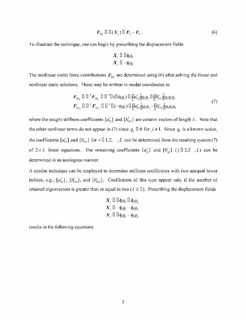
FNL [] [] (Xc) [] F_ -F L . (6)
TO illustrate the technique, one can begin by prescribing the displacement fields
xc _ D_ql
xc D-¢_ql
The nonlinear nodal force contributions F:vz are determined using (6) after solving the linear and
nonlinear static solutions. These may be written in modal coordinates as
FNq 0.0 _FNq 0.0 _.O(O_ql) O_all_qlq 10_blll_qlqlql
(7)FN_ a O.O_gN_a 0.0 _.O(-_q1)O _a11_qlql-_b111_qlqlql
where the sought stiffness coefficients [a_] and [bl_] are column vectors of length L. Note that
the other nonlinear terms do not appear in (7) since q/D 0 for j, 1. Since q_ is a known scalar,
the coefficients [a_] and [b_l] for r D 1,2, ,L can be determined from the resulting system (7)
of 2×L linear equations. The remaining coefficients [a{/] and [b_/] (jD 2,3 ,L) can be
determined in an analogous manner.
A similar technique can be employed to determine stiffness coefficients with two unequal lower
indices, e.g., [a_2 ] , [bi_2], and [bin]. Coefficients of this type appear only if the number of
retained eigenvectors is greater than or equal to two (L _ 2). Prescribing the displacement fields
X 00_q 10_2q2
x D-_ql-,_q_
x DD_ql-_q_
results in the following equations
FNZ_ [7 .[7 T.F]([].[_q 1 [7 []2q2) [7 _a(l_qlq 1 [7 _b(11_qlqlq1 [7 _a;2_q2q 2 D _b_22_q2q2q2
O _a(2_qiq 2 0 _b(12_qiqiq2 0 _b(22_qiq2q2
gNz _ [7 .[7 T.F]([].[_q 1 [7 .[]2q2) [7 _a(l_qlq 1 [7 _b(ll_qlqlql [7 _a_2_q2q 2 D _b_22_q2q2q2
O _a(2_qiq 2 0 _b(12_qiqiq2 0 _b(22_qiq2q2
gNz,3 [7 .[7 T.F]([].[_q 1 [7 .[]2q2) [7 _a(l_qlq 1 [7 _b(ll_qlqlql [7 _a_2_q2q 2 I7 _b_22_q2q2q2
O _a(2_qiq 2 0 _b(12_qiqiq2 0 _b(22_qiq2q2
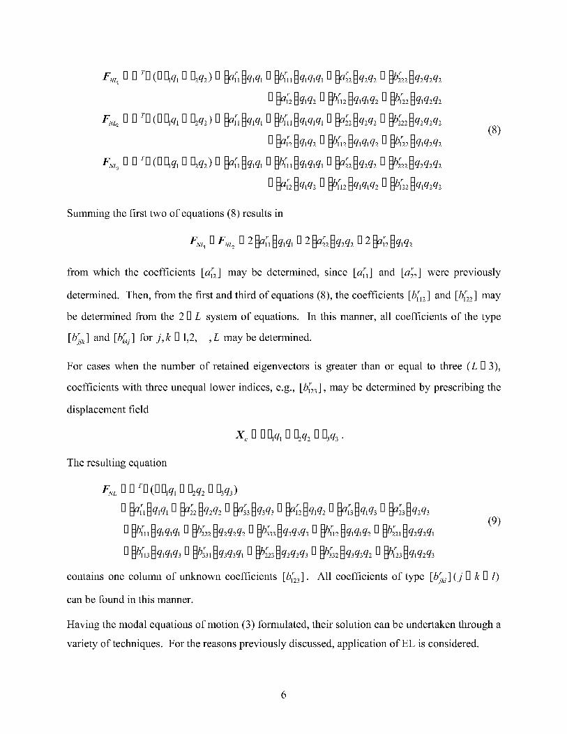
(8)
Summing the first two of equations (8) results in
FN_ [] FNL_ [] 2 _a(l _qlql [7 2 _a;2 _q2q2 [] 2 _a_2_qlq2
r r r
from which the coefficients [a12] may be determined, since [all ] and [a22 ] were previously
determined. Then, from the first and third of equations (8), the coefficients [b_rl2] and [b_r22] may
be determined from the 2 I7 L system of equations. In this manner, all coefficients of the type
[b_Tk] and [b_ki] for j,k [1 1,2, ,L may be determined.
For cases when the number of retained eigenvectors is greater than or equal to three (L I7 3),
coefficients with three unequal lower indices, e.g., [/)123], may be determined by prescribing the
displacement field
X [7 [].Olq1 [7 ._q2 [7 .[]3q3 •
The resulting equation
FN L [] .[] T.[]([].01ql [] []2q2 [] []3q3)
[7 [_alrl_qlql [7 _a;2_q2q 2 I7 [_a33_q3q 3 [7 _a_2_qlq 2 [7 [_alr3_qlq3 [7 _a;3_q2q 3
[7 _b_li_qiqiqi [7 _b_22_q2q2q2 I7 _b333_q3q3q3 I7 _b_12_qiqiq2 [7 _b221_q2q2qi(9)
[7 _b_13_qlqlq3 [7 _b331_q3q3q1 [7 _b;3_q2q2q 3 [7 _b332_q3q3q2 [7 _b(23_qlq2q3
contains one column of unknown coefficients [b1_3]. All coefficients of type [bill ] (j [] k [] l)
can be found in this manner.
Having the modal equations of motion (3) formulated, their solution can be undertaken through a
variety of techniques. For the reasons previously discussed, application of EL is considered.

3. EQUIVALENT LINEARIZATION APPROACH
An approximate solution to (1) can be achieved by formation of an equivalent linear system:
MX(t) 17CX(t) [3 (K [3Ke)X(t ) [3 F(t) (10)
where K is the equivalent linear stiffness matrix. While it is possible to perform an EL analysis
in the physical degrees-of-freedom, it is desirable to recast the problem in modal coordinates to
simplify the problem. The equivalent linear analog of equation (3) may be found by applying the
modal transformation (2) to (10):
M q [3 C q [3 _K [3Ke _q [3 F (11)
where the fully populated modal equivalent stiffness matrix is given by
K e [3 [3 rKe[3
Two EL approaches are considered. One is based on minimization of the error in the nonlinear
force vector and the other minimizes the error in potential (strain) energy.
3.1. FORCE-ERROR MINIMIZATION APPROACH
The traditional (force-error minimization) method of EL seeks to minimize the difference
between the nonlinear force and the product of the equivalent linear stiffness and displacement
response vector. Since the error is a random function of time, the required condition is that the
expectation of the mean square error be a minimum [3], i.e.
el'POP [3 E _([3 (X) [3 KeX) T ([3 ( X) [3 KeX)_'-'-_ rain (12)
where El...] represents the expectation operator. Equation (12) will be satisfied if
O(error) [3 0 i, j [3 1,2, , NOK..
e#l
where Kei j are the elements of matrix Ke, and N is the number of physical degrees of freedom.
In this study, consideration is limited to the case of Gaussian, zero-mean excitation and response
to simplify the solution. With these assumptions and omitting intermediate derivations, the final
form for the equivalent linear stiffness matrix in physical coordinates becomes (see for example
[4], [5]):

andin modalcoordinatesbecomes
o oo.ooOI_e O _E_]--_[_ (13)
o oo.ooOI_e O _ E _]--_q _ (14)
with 0 as previously defined in (4).
3.2. POTENTIAL ENERGY-ERROR MINIMIZATION APPROACH
An alternative EL approach based on potential (strain) energy-error minimization was proposed
in [6, 7]. Analysis in these works was limited to single degree-of-freedom systems and
simplified multiple degree-of-freedom systems. In this study, that approach is rigorously
generalized for the case of coupled multiple degree-of-freedom systems. One can begin with an
expression for the error in potential energy
error 1 T 20 Et(e(x)O-fx "eX) t (15)
where U(X) is the potential energy of the original (nonlinear) system. A condition of
minimized error requires that
°° tiE_t(U(X) O1XTKeX) 2 O0 i,j[] 1,2, ,N. (16)
Omitting intermediate derivations, one obtains the following system of N 2 linear equations with
respect to unknown elements of matrix K e :
N N
0 0 Ke,jE_xix.jxkx,_O 2E[xkx, U(X)] k,1 0 1,2, ,N. (17)i01 jOl
For example, equation (17) would have the following form for a two degree-of-freedom system
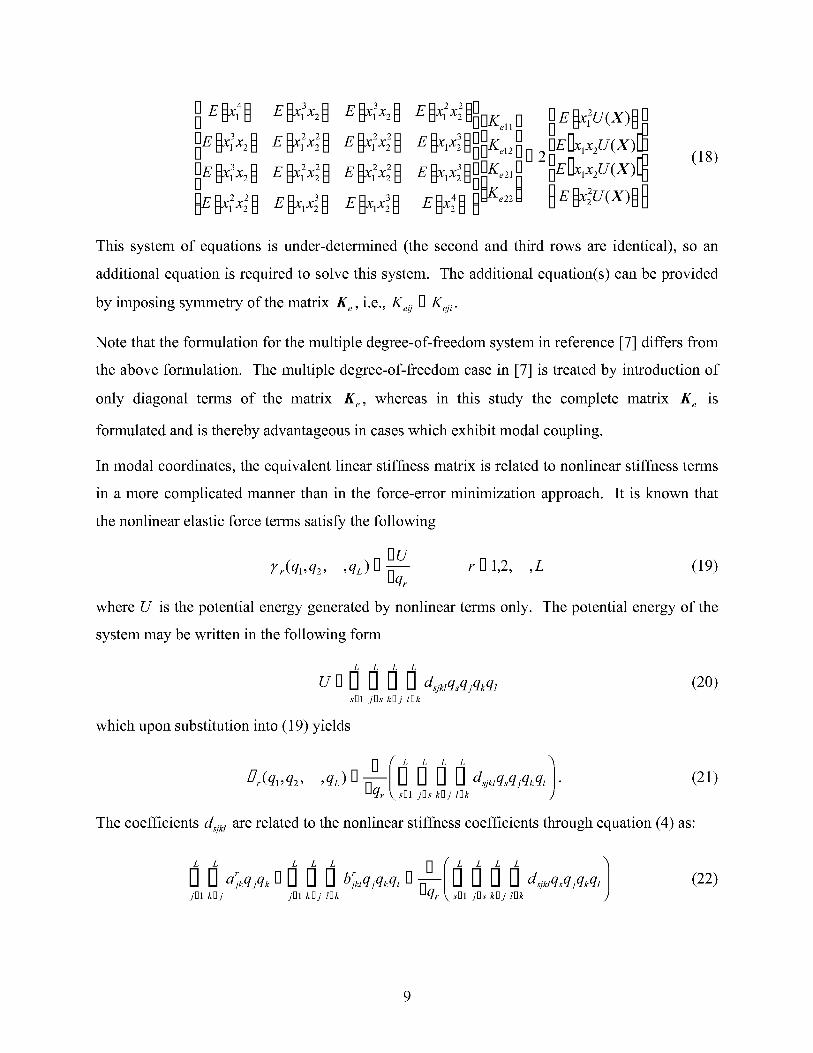
DE x4 ] E x x2 ]E x x2 ]D
D
D
_E_X2N2_ E_XIN_ E_NIN_
K DEgx U(X Dell [']
E_XIN_[qO0 K _ OEO)cIN2U(X)IF_
1113[] el2 i ['] 2 _E_71N2U(X)[ _
D_ X 3 [q[-][-]Ke21
E_]N4_] _ [=1/" e 22 _E_,y,2U(X)_]_
(18)
This system of equations is under-determined (the second and third rows are identical), so an
additional equation is required to solve this system. The additional equation(s) can be provided
by imposing symmetry of the matrix Ke, i.e., Kei i [] Kej i.
Note that the formulation for the multiple degree-of-freedom system in reference [7] differs from
the above formulation. The multiple degree-of-freedom case in [7] is treated by introduction of
only diagonal terms of the matrix l_e, whereas in this study the complete matrix i_ e is
formulated and is thereby advantageous in cases which exhibit modal coupling.
In modal coordinates, the equivalent linear stiffness matrix is related to nonlinear stiffness terms
in a more complicated manner than in the force-error minimization approach. It is known that
the nonlinear elastic force terms satisfy the following
DU7r(q,,q2, ,qL) [] -- r [] 1,2, ,L (19)
Flqr
where U is the potential energy generated by nonlinear terms only. The potential energy of the
system may be written in the following form
L L L L
U D F] F] F] F] d,;kzq,q./qkqz (20)slql jlqs k[]j l[]k
which upon substitution into (19) yields
g(q,,q2, ,qc) [] [] 0 0 d_/k,q,q/qkq, • (21)slql jlqs k[]j l[]k
The coefficients d_ikl are related to the nonlinear stiffness coefficients through equation (4) as:
.jD1 kD.j " " .jD1kD.i /Dk " " Uqr _ sD1 .jDs kD.j l_k " "
(22)

In the following, a zero-meanresponseis assumed,i.e., E[q] rl o. As will be subsequently
shown, this has the effect of dropping out the quadratic terms ajk. From (22), the coefficients
d,jkl can then be written as:
[b)_k,/ 2 s [] j/
d_Jk, [] _b)_k,/3 s [] j [] k (23)
_ I /b,;,/4 sD#D Dztb)_k, otherwise.
Note that if the zero-mean response assumption were not made, the above relationship would be
more complicated. Having U now fully defined from equation (20), the modal equivalent of
equation (17) can be written as
L L
0 0 Kei/E_qiq./qkql_[] 2E[]clkqzU(q)_ k,l[] 1,2, ,L (24)iD1 jD1
from which K ecan be determined. The matrix on the left hand side of equation (24) involves 4 th
order moments of modal displacements. The right hand side involves 4th, 5 th and 6 th order modal
displacement moments since the potential energy is a function of the 2 nd, 3 rd, and 4 th order
displacements. Assuming a Gaussian distributed, zero-mean response, the odd order moments
are zero and the higher order even moments can be expressed in terms of the 2 nd order moments.
For example,
E_qiq./qkqz_ lq E_qiq./_E[qkqz_ lqE[qiqk_E_q./qz_ lq E[qiqz_E_q./qk_.
Therefore, the matrices of equation (24) can be written solely in terms of the modal response
covariance.
4. ITERATIVE SOLUTION
Because the modal equivalent linear stiffness matrix /£e
displacements, the solution takes an iterative form.
displacements and forces may be expressed as:
q(t) D 0 gleiu°'n
is a function of the unknown modal
The time variation of the modal
f(t) [] 0 J¢eiu°t (25)n
10

where(A) indicatesthe dependencyon con. Applying (25) to (11) and writing in iterative form
gives:
4 m 0 HmDlf (26)
where m is the iteration number and
H mm DEDff2MDiffnCDKD[c_KmnlD flKmn2]_ _ (27)
The introduction of the weightings a and fl are to aid in the convergence of the solution, with
the condition that a _ fl D 1.
For stochastic excitation, (26) is rewritten as:
SqOHm°lSfEHm°l _
and the r,s component of the covariance matrix of modal displacements is
E[qrq,[_ D 0 S2qAQnn
(28)
Here, Sq is the spectral density matrix of modal displacements and S 1 is the spectral density
matrix of the load in modal coordinates. The diagonal elements, Sqrqr, are the variances of the
modal displacements. K e is zero for the first iteration, which yields the covariance matrix
E[q,.q,] of the linear system. For subsequent iterations (re>l), the nonlinear stiffness depends on
the minimization approach taken.
For example, for the force-error minimization approach, K e for the m th iteration is determined
from (14) as
SF D[]___S DOl Sm[]L, U Dqlu "'" E _-q_ RI-1
_ DrlrlDDmKm 0 _n-O[ ] 0 0 " ". " 0e D rluqrlFl rl " S
_E DD_-_-_S ... E D_-_-_SDU nqt U UnqLU_
(29)
Substitution of equation (4) into (29) gives
11

nno_°_a,,'E_e,_Or] r] b;_mE_e,e_ r] aJ_'E_q,_Or] r]0 j .iN kDj j .iN kDj
Kf [] []D
I! L L L L LajlE b.jklE _q.jqk _ 0 a.jLE _.j _ [] 0 0
.iN kD.j j .iN kD.j
DDD
bj_E_]qjqk_] I
Since a zero-mean response is assumed, i.e. E[q] r] 0, equation (30) reduces to:
(30)
0 L 0 roD1
O0 rl b._kmE _q./qk _ rl rl b.ljkLE _q./qk _O
O.]D1 kll j .][]1 kll j 0
rl rlK'_ [] [] L L []
°! D_. 1 kDj .]D1 kDj
(31)
For the potential energy-error minimization approach, K e is found by solving the system of
equations (24) in a similar iterative fashion.
For both error minimization approaches, the iterations continue until convergence of the modal
equivalent linear stiffness matrix such that
Kme 0 K_ D1 < E
The value of c typically used is 0.1%.
Following convergence, the N x
coordinates is recovered from
N covariance matrix of the
E_x_x/_O 0 ECq,q, O0_
displacements in physical
(32)
Furtherand root-mean-square (RMS) values are the square roots of the diagonal terms in (32).
post-processing to obtain power spectral densities of displacements, stresses, strains, etc., may be
performed by substituting the converged equivalent stiffness matrix into (11) and solving in the
usual linear fashion.
5. IMPLEMENTATION
The EL procedures as outlined above were recently implemented within the context of
MSC.NASTRAN [10] version 70.0 (heretofore NASTRAN) using the DMAP programming
language [15]. Its operation has been verified through NASTRAN version 70.7. Details of these
12
implementations,collectively calledELSTEP for "Equivalent Linearizationusing a STiffness
EvaluationProcedure,"aredocumentedin [16]. The implementationsentail first performinga
normalmodesanalysis(solution 103)to obtainthe modal matrices,from which a subsetof L
modes are chosen. The nonlinear stiffness coefficients are then determined by performing a
series of linear static (solution 101) and nonlinear static (solution 106) solutions using linear
combinations of modes as previously described. The iterative solution is performed in a
standalone routine, which has as its output the RMS displacements in physical coordinates, the
cross covariance in modal coordinates, and the sum of the linear and equivalent linear modal
stiffness matrices. The latter can then be substituted for the linear modal stiffness in the modal
frequency response analysis (solution 111) for post-processing.
6. NUMERICAL SIMULATION ANALYSIS
For validation purposes, a numerical simulation analysis was performed to generate time history
results from which response statistics could be calculated. The particular method used was finite
element-based with the integration performed in modal coordinates, as described in [14]. The
finite element model uses the 4-node, Bogner-Fox-Schmit (BFS) C 1 conforming rectangular
element with 24 degrees-of-freedom: 4 bending degrees-of-freedom (w, D_x, D_y, D2_fDxDy)and 2
in-plane degrees-of-freedom (u,v) at each node. The equations of motion are derived using the
von Karman large deformation theory. In applying this modal approach, the modal truncation
should be the same as that used in the EL approach.
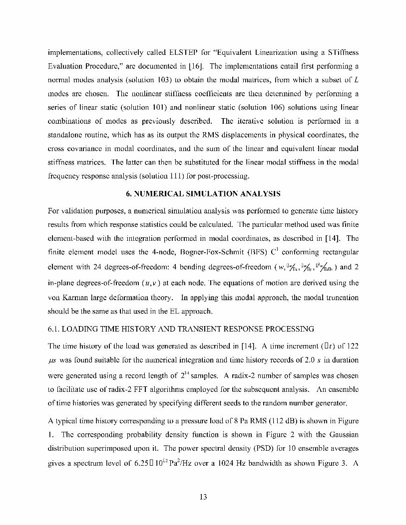
6.1. LOADING TIME HISTORY AND TRANSIENT RESPONSE PROCESSING
The time history of the load was generated as described in [14]. A time increment (_t) of 122
/Js was found suitable for the numerical integration and time history records of 2.0 s in duration
were generated using a record length of 2 TM samples. A radix-2 number of samples was chosen
to facilitate use of radix-2 FFT algorithms employed for the subsequent analysis. An ensemble
of time histories was generated by specifying different seeds to the random number generator.
A typical time history corresponding to a pressure load of 8 Pa RMS (112 dB) is shown in Figure
1. The corresponding probability density function is shown in Figure 2 with the Gaussian
distribution superimposed upon it. The power spectral density (PSD) for 10 ensemble averages
gives a spectrum level of 6.25 D 10 D=PaZ/Hz over a 1024 Hz bandwidth as shown Figure 3. A
13

sharproll-off of the input spectrumpracticallyeliminatesexcitationof the structureoutsidethe
frequencyrangeof interest.
Thestructureis assumedto beatrestat thebeginningof eachloading. An initial transientin the
structuralresponseis thereforeinducedbefore the responsebecomesfully developed. This
transientmustbeeliminatedto ensuretheproperresponsestatisticsarerecovered.In the linear
case,a moving block averageof 1.0sof datawas usedto ascertainthe point in the recordat
which the RMS displacementresponsebecamestable.In this manner,it was determinedthat
eliminationof thefirst 1.0sof the2.0srecordwasmorethansufficient. While thesamecriterion
doesnot strictly apply to thenonlinearresponsecasebecauseof thedependenceof theresponse
on theinitial conditions,it wasemployedwith satisfactoryresults.
14

30
20
10
"0
0•_ 0
•_ -lOa.
-20
-300 0.5 1 1.5 2
Time (s)
Typical acoustic loading time history.Figure 1:
0.06
II Load Distribution- Normal Distribution
0.05
0.04
_0.03
0.02
£a.
O.Ol
_.._d IN
_-30 -20 -10 0 10 20 30
Distribution Range (Pa)
Figure 2: Typical probability density of acoustic loading.
15

10-1
N"1-
GIoo
1o-3
1o-5
10 -7 --
10.9 _
10-110
I I I I I I I I I I I I I I I500 1000 1500
Frequency (Hz)
Figure 3: Typical averaged power spectral density of acoustic loading.
6.2. RESPONSE STATISTICS
Response statistics were generated from an ensemble of N=10 time histories at each load level.
Estimates of the displacement RMS served as the basis for comparison with the EL method.
Additionally, confidence intervals for the mean value of the displacement RMS estimate were
generated to quantify the degree of uncertainty in the estimate [ 17] using:
2. rl ---_- rl Jux rl 2. rl ---F_ , n rl N rl l (33)
where 2- and s 2 are the sample mean and variance of the RMS estimates from N ensembles, and
tn is the Student t distribution with n degrees of freedom, evaluated at 6, / 2. For the 90% confi-
dence intervals calculated, 6, _ 0.1.
Estimates of the displacement mean, skewness, and kurtosis were also computed to help
ascertain the degree to which the assumptions made in the development of the EL method were
followed. Power spectral density and probability density functions (PDF) of the displacement
were computed for similar purposes.
16
7.RESULTS
Validation studieswere conductedusing a rectangularaluminumplate measuring0.254m x
0.3556mof thickness,h, 0.00102m. All sides were simply supported. The material properties
used were:
E [] 7.3 [] 101°Pa, v [] 0.3, p [] 2763 kgm 3
where E is the elastic modulus, v is Poisson's ratio, and p is the mass density. The plate was
subjected to a spatially-uniform pressure loading over a computational bandwidth of 1024 Hz, as
shown in Figure 1. Since the loading was uniformly distributed, only symmetric modes were
included in the analysis. In general, any combination of symmetric and non-symmetric modes
may be included.
A NASTRAN model of the full plate was built with 560 CQUAD4 elements measuring 0.0127m
square for use in the EL analysis. The first two symmetric modes (modes 1 and 4) of this model
had natural frequencies of 58.38 and 217.27 Hz. For comparison, the natural frequencies given
by an analytical solution [18] were 58.34 and 216.01 Hz for the first two symmetric modes.
These two modes were selected as participating modes in the EL and numerical simulation
analyses. Modal damping was chosen to be sufficiently high (2.0% and 0.54% critical damping)
so that a good comparison with the numerical simulation results could be made at the peaks of
the PSD. The finite element model used in the numerical simulation analysis had the same
element size (0.0127m square) as the NASTRAN model, but a quarter-plate model was used to
reduce computational time. This model gave natural frequencies of 58.12 and 215.19 Hz for the
first two symmetric plate modes. Both EL and simulation finite element models were checked
for convergence by running additional analyses with models consisting of 0.00635m elements.
Analysis was performed at overall sound pressure levels from roughly 106 dB (4 Pa RMS) to
roughly 160 dB (2048 Pa RMS), in 6 dB increments, giving a dynamic range of 54 dB. Figure 4
shows the normalized RMS out-of-plane (w) deflection at the plate center as a function of
loading. Both force-error and potential energy-error minimization implementations are shown.
The numerical simulation results are shown with 90% confidence intervals of the RMS estimate.
At the lowest load level of 106 dB, the response is linear as can be seen by the comparison with
17

results from a strictly linear analysis (NASTRAN solution 111). Small, but noticeable,
differences between the linear and nonlinear responses are noted at the 118 dB load level. The
degree of nonlinearity increases with load level, as expected. At the highest level of 160 dB, the
nonlinear response calculations predict RMS center deflections of 2.20 and 2.27 times the
thickness for the force and potential energy-error minimization approaches, respectively. The
90% confidence interval on the numerical simulation data by comparison is 2.24 < WRMs/h < 2.39
at 160 dB. Consistent with past observations [11, 12], potential energy-error minimization
results are closer to known solutions and somewhat higher (by a few percent) than force-error
minimization results. The linear analysis by comparison predicts center deflections of nearly 13
times the thickness.
e- 100
10-1
.......... Linear
101 ELSTEP Force /ELSTEP Potential Energy ,,/'
/....... SEMELRR /"
• Simulation //,'
/ I /z/ .J
/,. j.j.i
/"./"
.6" /
100 110 120 130 140 150 160 170
Acoustic Load (dB)
Figure 4: Normalized RMS center deflection as a function of acoustic load.
Results from the earlier SEMELRR implementation [9], also shown in Figure 4, were generated
with the same NASTRAN model. These results are shown to significantly over-predict the
effect of nonlinearity at loads as low as 124 dB. At 160 dB, the SEMELRR implementation
predicts an RMS center deflection of 1.38 times the thickness, or approximately 60% less than
18

the mean of the numericalsimulation prediction. The highly non-conservativenatureof the
SEMELRRanalysismakesit unsuitablefor nonlinearstructuraldesign.
In orderto gain greaterinsight into the nonlineardynamics,plotsof thetime history, PDF,and
PSDareshownfor threeload levels,(106, 136 and 160dB) in the following seriesof figures.
Datain the time historyandPDF plotscorrespondsolely to numericalsimulationresults. Data
in thePSDplots correspondto numericalsimulationandEL results,wherethe EL resultswere
generatedby running a linear analysis(NASTRAN solution 111) usingthe modal equivalent
linearstiffnessK e generated by the EL process previously described.
Results for the 106 dB excitation level are shown in Figure 5 - Figure 7. This excitation level
was shown (see Figure 4) to produce a linear response. As expected, the PDF mimics the
normally distributed PDF of the input shown in Figure 1. The averaged PSD shows excellent
agreement between the EL, linear, and numerical simulation results. This agreement helps to
establish the confidence in making comparisons between these two fundamentally different
analyses.
0.1
A
E o.o5E
e,-
E
O0
.__121
e,--0.05
O
-0.10 0.25 0.5 0.75 1
Time (s)
Figure 5: Time history of center displacement response at 106 dB.
19

20-
- II w Distribution18 - - Normal Distribution
16-
14-
.._ 12
lO
£D.
°o 1Distribution Range (mm)
Figure 6: Probability density of center displacement response at 106 dB.
10 -9 m
AN
E
a
1o -_a
@
E@(,)
10 -1_ -
.__a¢_@
10 -17e-
U
10 -190
i .......... Linear................... ELSTEP Force
.......................ELSTEP Potential EnergyNumerical Simulation
i i i i I i i i i I i i i i I i i i i I250 500 750 1000
Frequency (Hz)
Figure 7: Power spectral density of center displacement response at 106 dB.
20

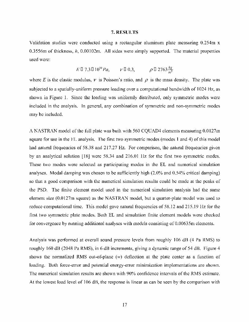
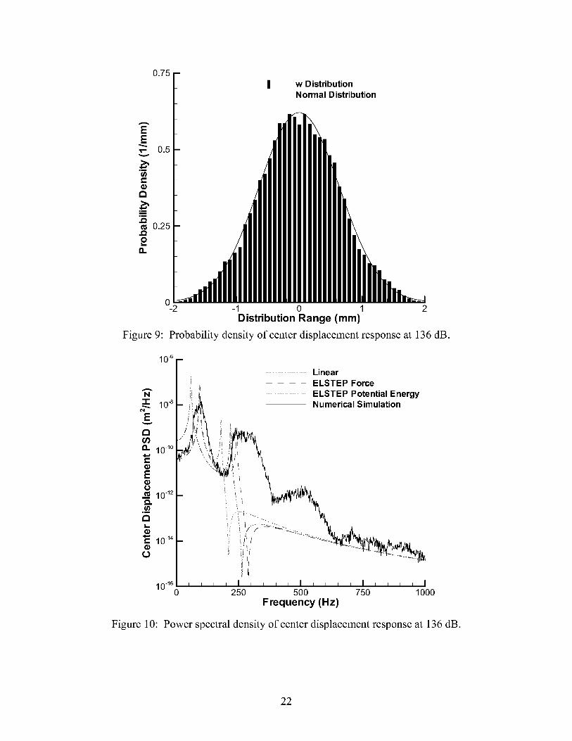
Figure 8 - Figure 10 show the nonlinear response associated with the 136 dB excitation level.
The time history of the center displacement has a visibly higher peak probability and the PDF
exhibits a minor flattening at the peak. The shapes of the PSDs from the EL analyses are those
of the equivalent linear systems. Thus, the PSDs from the EL analyses do not show the peak
broadening effect observed in the numerical simulation. Additionally, harmonics in the
structural response are present only in the numerical simulation results. The PSDs from both the
numerical simulation and EL analyses show a positive shift in the frequency of the fundamental
mode compared with the linear solution. Both EL analyses shift the fundamental frequency by
nominally the same amount and fall within the broadening fundamental peak of the numerical
simulation analysis. The frequency of the second mode from the force-error minimization
analysis also increases and more closely matches the numerical simulation data than does the
potential energy-error minimization analysis, which shows a negative frequency shift.
2
-20 0.25 0.5 0.75 1
Time (s)
Figure 8: Time history of center displacement response at 136 dB.
21
0.75
w Distribution
Normal Distribution
EE
•- 0.5
e"
GI
,m
.O0.25
.ola.
0-2 -1 0 1 2
Distribution Range (mm)
Figure 9: Probability density of center displacement response at 136 dB.
10 -6
10 -16
0
........................ Linear
ELSTEP Force
................... ELSTEP Potential EnergyNumerical Simulation
Figure 10: Power spectral density of center displacement response at 136 dB.
22
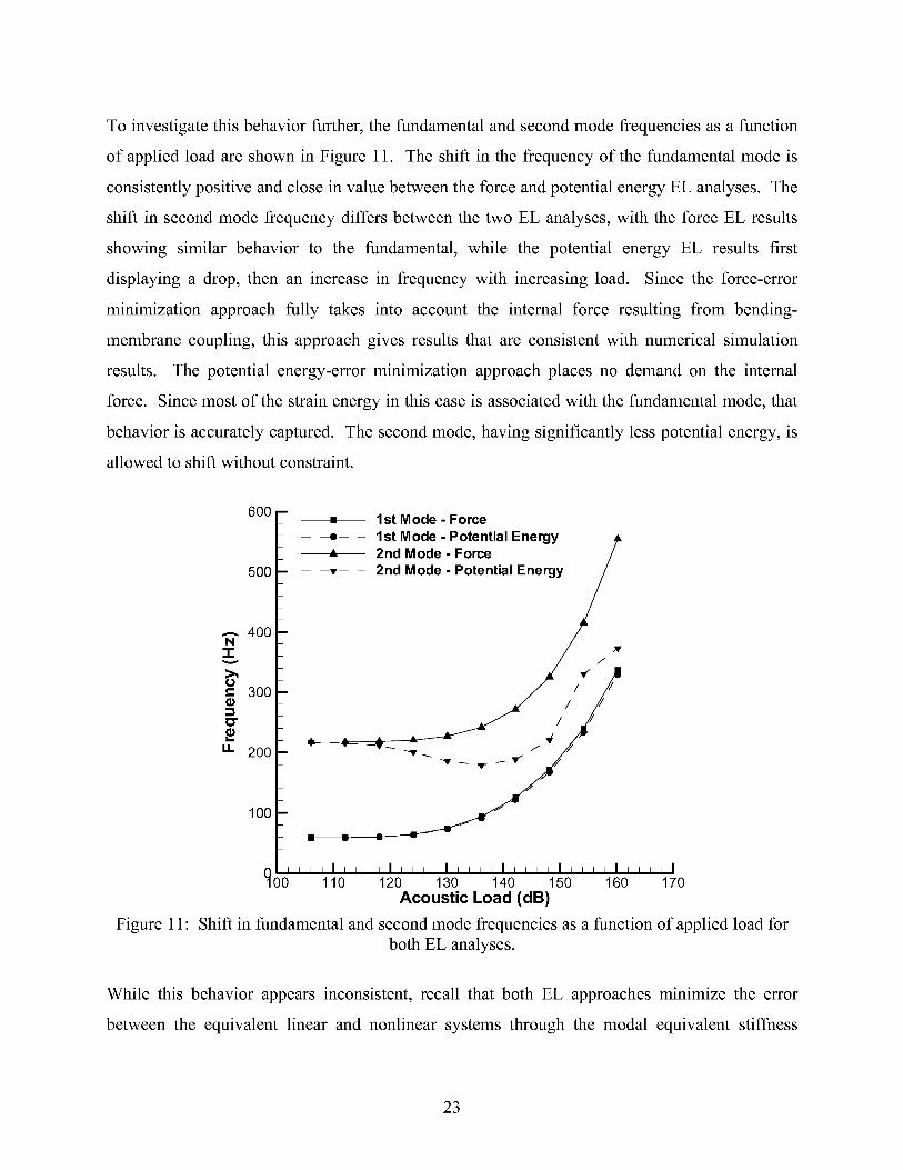
To investigate this behavior further, the fundamental and second mode frequencies as a function
of applied load are shown in Figure 11. The shift in the frequency of the fundamental mode is
consistently positive and close in value between the force and potential energy EL analyses. The
shift in second mode frequency differs between the two EL analyses, with the force EL results
showing similar behavior to the fundamental, while the potential energy EL results first
displaying a drop, then an increase in frequency with increasing load. Since the force-error
minimization approach fully takes into account the internal force resulting from bending-
membrane coupling, this approach gives results that are consistent with numerical simulation
results. The potential energy-error minimization approach places no demand on the internal
force. Since most of the strain energy in this case is associated with the fundamental mode, that
behavior is accurately captured. The second mode, having significantly less potential energy, is
allowed to shift without constraint.
600 -
5OO
.-, 400N-1-
e- 300
O"
u. 200
100
" 1st Mode - Force
-- --=-- - 1st Mode - Potential Energy
-- 2--- _nddMo°dd:_F;rt;ential Ene /rg_.v
,,,,,I,,,,I,,,,I,,,,I,,,,I,,,,I,,,,I
[J00 110 120 130 140 150 160 170
Acoustic Load (dB)
Figure 11: Shift in fundamental and second mode frequencies as a function of applied load for
both EL analyses.
While this behavior appears inconsistent, recall that both EL approaches minimize the error
between the equivalent linear and nonlinear systems through the modal equivalent stiffness
23

matrix Ke, which is a function of the modal displacement. It is therefore expected that only the
RMS displacement, or the area under the displacement PSD, should be the same between either
EL analysis and the numerical simulation analysis, and not the shape of the PSD itself. This is
consistent with the observations.
The highest degree of nonlinearity is shown in Figure 12 - Figure 14, corresponding to a 160 dB
acoustic load. The time history is further peak oriented and the PDF exhibits substantial
flattening. The peak broadening in the PSD of the numerical simulation results is severe, and
nearly flattens the spectrum above 350 Hz. With regard to the EL analyses, positive shifts in the
frequencies of the fundamental mode are comparable between the two EL analyses. Shifts in the
second mode frequencies are more substantial in the force-error minimization approach than in
the potential energy-error minimization.
8
6
-8 o
Figure 12:
0.25 0.5 0.75 1
Time (s)
Time history of center displacement response at 160 dB.
24

0.2
w Distribution
Normal Distribution
A
E o.15E
,,,,.,,,,
._z,c
0.1a
,m
2 0.050,.
0-8 -4 0 4 8
Distribution Range (mm)
Figure 13: Probability density of center deflection response at 160 dB.
10 -4 --
AN
•1- 10 .6
E
13t_
10 .8
Eo
10 -1°
.__13
""= 10 -12
0
_L
-i! 'i!!!t
.......... Linear
ELSTEP Force
....................... ELSTEP Potential EnergyNumerical Simulation
'I
/
_-: - " t • t..... -:it . --" , i t
I/ .......: ....
il i /i
q
10 -14 I I I I I I I I I I I I I I I I I I I I0 250 500 750 1000
Frequency (Hz)
Figure 14: Power spectral density of center deflection response at 160 dB.
25

Momentsof thecenterdisplacementwerecalculatedfrom thenumericalsimulationresultsfor all
load levels. They areprovided in Table 1 with the RMS centerdisplacementfrom both EL
analyses.TheEL andnumericalsimulationresultsagreewell, thusvalidating theEL analysis
overa substantialloadrange. Thevalidity of assumptionsmadein the developmentof the EL
method is ascertainedby observingthe mean,skewnessand kurtosis. The mean value is
effectivelyzerofor all loadlevels,indicatingtheassumptionof zeromeanresponsehasnot been
violated. Although thePDF is moreor lessskew-symmetric,theshapeis flattenedat thehigher
load levels as indicatedby a decreasingkurtosis from the linear value of 3. The decreasing
kurtosisvaluesindicatea violation of the Gaussianresponseassumption.However,evenwith
this non-Gaussianresponsedistribution, the EL analysesgive good predictionsof the RMS
response.
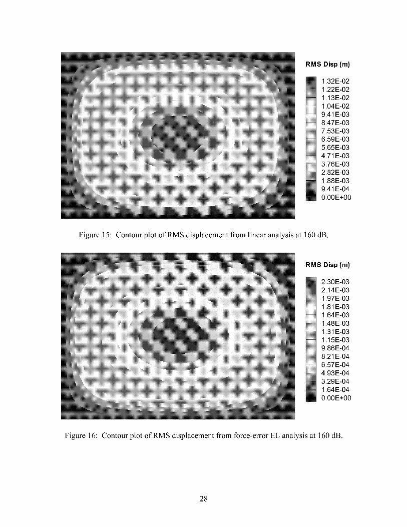
Plotsof the RMS displacementover the entireplate areshownin Figure 15 - Figure 17 for the
linearandEL analysesfor the 160dB loadcase.While theplotsappearsimilar in character,the
linear displacementcontours look rounder than those of the two EL analyses. To better
understandthenatureof thesedifferences,theRMS displacementswerenormalizedwith respect
to theirmaximum(center)displacementfor eachof thethreecases.Thedifferencesbetweenthe
normalizedlinearandforce-errorminimizationEL displacements,andthenormalizedlinearand
potential energy-errorminimization EL displacementsare shown in Figure 18 - Figure 19.
Theseareexpressedin percentwith respectto the maximumnormalizeddisplacement(unity).
In eachcase,the greatestdifferenceoccursalong the horizontal centerlineand nearthe short
sidesof theplate. Theseplotshighlight theneedto performa nonlinearanalysisto obtainthe
properspatialdistribution. As previouslynoted,the differencebetweenthe two EL analysesis
smallrelativeto their displacement,asshownin Figure20. Thedifferenceresemblesthesecond
symmetricmode. This observationis consistentwith thePSDin Figure 14,which indicatesthe
maximummagnitudedifferencebetweenthe two EL analysesto be associatedwith the second
mode.
26

Table 1: Moments of the center displacement.
Load
(dB)
106
112
118
124
130
136
142
148
154
160
Force Error
EL RMS (m)
2.57x10⁴
5.12x10⁴
1.00xl0 -4
1.88x10 -4
3.24x10 -4
5.13x10 -4
7.68x10 -4
1.10xl0 -3
1.58x10 -3
2.25x10 -3
Potential Energy
Error EL RMS (m)
2.57x10⁴
5.12x10⁴
1.01x10 -4
1.90x10 -4
3.30x10 -4
5.27x10 -4
7.95x10 -4
1.16x10 -3
1.63x10 -3
2.32x10 -3
SEMELRR Num Sim
RMS (m) Mean (m)
2.56x10⁴ +1.56x10 -7
5.04x10 -s +3.07x10 -7
9.54x10 -s +l.01xl0 -8
1.66x10⁴ +7.94x10 -7
2.62x10⁴ +1.87x10 -6
3.84x10⁴ -5.23x10 -7
5.35x10⁴ -3.18x10 -7
7.27x10⁴ +2.58x10 -6
1.05x10 -3 +l.04x10 -6
1.41x10 -3 +6.05x10 -6
Numerical Simulation RMS (m)
(90% Confidence Interval)
2.37x10⁴[] RMS < 2.76x10⁴
4.68x10-s[] RMS < 5.47x10 -s
9.34x10-s[] RMS < 1.06x10 -4
1.76x10⁻⁴[] RMS < 1.96x10 -4
3.42x10⁻⁴[] RMS < 4.01x10 -4
6.09x10⁻⁴[] RMS < 6.71x10 -4
8.38x10⁻⁴[] RMS < 9.30x10 -4
1.14x10⁻³[] RMS < 1.26x10 -3
1.61x10⁻³[] RMS < 1.79x10 -3
2.29x10⁻³[] RMS < 2.44x10 -3
Skewness Kurtosis
+0.0017 3.21
+0.0013 3.18
+0.0012 2.90
+0.0027 2.60
-0.0010 2.81
+0.0033 2.83
+0.0032 2.48
-0.0063 2.38
+0.0012 2.36
-0.0061 2.28
27
RMS Disp (m)
1.32E-021.22E-021.13E-021.04E-029.41E-038.47E-037.53E-036.59E-035.65E-034.71E-033.76E-032.82E-031.88E-039.41E-040.00E+00
Figure 15: Contour plot of RMS displacement from linear analysis at 160 dB.
RMS Disp (m)
2.30E-032.14E-031.97E-031.81E-031.64E-031.48E-031.31E-031.15E-039.86E-048.21E-046.57E-044.93E-043.29E-041.64E-040.00E+00
Figure 16: Contour plot of RMS displacement from force-error EL analysis at 160 dB.
28

RMS Disp (m)
2.30E-032.14E-031.97E-031.81E-031.64E-031.48E-031.31E-031.15E-039.86E-048.21E-046.57E-044.93E-043.29E-041.64E-040.00E+00
Figure 17: Contour plot of RMS displacement from potential energy-error EL analysis at 160dB.
Percent RMSDisplacementDifference
5.405.014.624.243.853.463.072.692.301.911.521.130.750.36
-0.03
Figure 18: Difference between normalized linear and force-error EL displacements at 160 dB.
29

Percent RMSDisplacementDifference
7.807.146.495.835.174.513.863.202.541.891.230.57
-0.09-0.74-1.40
Figure 19: Difference between normalized linear and potential energy-error EL displacements at160 dB.
RMSDisplacementDifference (m)
0.00E+00-7.75E-06-1.55E-05-2.32E-05-3.10E-05-3.87E-05-4.65E-05-5.42E-05-6.20E-05-6.97E-05-7.75E-05-8.52E-05-9.30E-05-1.01E-04-1.08E-04
Figure 20: Difference between displacements from force-error and potential energy-error
minimization analyses at 160 dB.
30

8. DISCUSSION
Differences between the two EL analyses and the numerical simulation do exist and warrant
some discussion. It is seen that the EL approach slightly over-predicts the degree of nonlinearity
compared to the numerical simulation results. Interestingly, the greatest differences appear in
the moderately nonlinear regime. The differences do not appear to be due to a violation of the
assumption of a Gaussian response because the over-prediction does not correlate with
increasing kurtosis of response. The trends observed here are consistent with comparisons
between a different numerical simulation analysis and a force-error minimization EL analysis of
a clamped-clamped beam [13]. Comparisons of the force and potential energy-error
minimization approaches with an F-P-K solution of a beam, however, indicate that EL solutions
span the exact solution, with the potential energy-error minimization results being slightly higher
and the force-error minimization results being slightly lower than the exact solution [12]. It
would therefore appear that the numerical simulation solutions are less stiff than the EL solutions
in the moderately nonlinear regime, but this has yet to be fully substantiated.
Some implications on the use of the EL technique as a basis for fatigue life calculations are
worth mentioning. First, assuming that stresses or strains from the EL technique will compare
equally well with those from the numerical simulation analysis, a simple fatigue-life calculation
based on RMS levels will be much less conservative than calculations based on linear analyses.
This offers the potential for substantial weight savings for structures designed using nonlinear
methods. Secondly, it appears that a nonlinear analysis, EL or otherwise, is required to accurately
calculate the RMS deflected shape. Use of a linear RMS deflected shape scaled to the nonlinear
level would inaccurately reflect the spatial distribution. Simple fatigue-life calculations based on
the RMS stress or strain could be significantly affected as these quantities depend on the spatial
distribution of the deformation. Lastly, use of the EL-derived PSD response in a more
sophisticated fatigue-life calculation requires careful investigation. Recall that peaks in the
equivalent linear PSD may occur at different frequencies than in the PSD from the numerical
simulation analysis, as shown in Figure 10 and Figure 14. Methods such as spectral fatigue
analysis [19], which take moments of the PSD, may incorrectly account for the contribution of a
particular frequency component in the cycle counting scheme. It is not known, for example, if
the narrowly shaped, higher fundamental frequencies of the equivalent linear PSD result in
31
conservativeor non-conservativeestimatesof fatiguelife relativeto predictionsmadeusingthe
numerical simulation PSD with more broadly shaped,lower fundamentalfrequencies. An
assessmentof this effectis left asanareafor furtherstudy.
9. CONCLUSIONS
A novel methodfor determiningnonlinearstiffnesscoefficientsof arbitrarystructureshasbeen
developed.Themethodcanbe implementedin any finite elementcodehavinga geometrically
nonlinearstatic capability. It hasbeenimplementedasa DMAP alter to MSC.NASTRANto
demonstrateits effectiveness.
A potential energy-errorminimization EL approachhas been extendedto handle multiple
degree-of-freedomsystems.The RMS randomresponsepredictionsfrom it and the traditional
force-errorminimization approachhavebeenvalidatedthrough comparisonwith a numerical
simulationmethodover a wide rangeof load levels. Comparisonswith numericalsimulation
resultsaregood,evenwhenthe assumptionof Gaussianresponsehasbeenviolated. It hasbeen
shown that a linear analysisgrossly over-predictsthe RMS displacements(i.e., it is too
conservative)in comparisonwith numerical simulation results. The potential energy-error
minimization approachprovided a slightly more conservativeestimateof RMS displacement
than the force-error minimization approach. It was demonstratedthat an earlier EL
implementation(SEMELRR)significantly over-predictstheeffectof nonlinearity(i.e., it is non-
conservative).
ACKNOWLEDGEMENTS
The authors wish to acknowledge the contributions of Jean-Michel Dhainaut and Professor Chuh
Mei at Old Dominion University in generating the numerical simulation results under NASA
grant NAG-I-2294. The authors also wish to thank Travis L. Turner and Jay H. Robinson of the
Structural Acoustics Branch at the NASA Langley Research Center for helpful discussions and
comments.
REFERENCES
[1] Bolotin, V.V., Statistical methods in structural mechanics, Holden-Day, Inc., 1969.
32
[2] Lin, Y.K., Probabilistic Theory of Structural Dynamics. Malabar, FL, R.E. Krieger,1976.
[3] Caughy, T.K., "Equivalent linearization techniques," Journal of the Acoustical Society of
America, Vol. 35, pp. 1706-1711, 1963.
[4] Roberts, J.B. and Spanos, P.D., Random vibration and statistical linearization. New
York, NY, John Wiley & Sons, 1990.
[5] Atalik, T.S. and Utku, S., "Stochastic linearization of multi-degree-of-freedom nonlinear
systems," Earthquake engineering and structural dynamics, Vol. 4, pp. 411-420, 1976.
[6] Elishakoff, I. and Zhang, R., "Comparison of new energy-based versions of the stochastic
linearization technique," IUTAMSymposium, Springer-Verlag, pp. 201-211, Turin, 1992.
[7] Fang, J. and Elishakoff, I., "Nonlinear response of a beam under stationary excitation by
improved stochastic linearization method," Applied Mathematical Modelling, Vol. 19, pp.
106-111, 1995.
[8] Chiang, C.K., Mei, C. and Gray, C.E., "Finite element large-amplitude free and forced
vibrations of rectangular thin composite plates," Journal of Vibration and Acoustics, Vol.
113, No. July, pp. 309-315., 1991.
[9] Robinson, J.H., Chiang, C.K., and Rizzi, S.A., "Nonlinear Random Response Prediction
Using MSC/NASTRAN," NASA TM-109029, October 1993.
[10] "MSC/NASTRAN Quick Reference Guide, Version 70.5," MacNeal Schwendler
Corporation, 1998.
[11] Muravyov, A.A., Turner, T.L., Robinson, J.H., and Rizzi, S.A., "A New Stochastic
Equivalent Linearization Implementation for Prediction of Geometrically Nonlinear
Vibrations," Proceedings of the 40th AIAA/ASME/ASCE/AHS/ASC Structures, Structural
Dynamics and Materials Conference, Vol. 2, AIAA-99-1376, pp. 1489-1497, St. Louis,
MO, 1999.
[12] Muravyov, A.A., "Determination of Nonlinear Stiffness Coefficients for Finite Element
Models with Application to the Random Vibration Problem," MSC Worldwide Aerospace
Conference Proceedings, MacNeal-Schwendler Corp., Vol. 2, pp. 1-14, Long Beach,1999.
[13] Rizzi, S.A. and Muravyov, A.A., "Comparison of Nonlinear Random Response Using
Equivalent Linearization and Numerical Simulation," Structural Dynamics: Recent
Advances, Proceedings of the 7th International Conference, Vol. 2, pp. 833-846,
Southampton, England, 2000.
[14] Mei, C., Dhainaut, J.M., Duan, B., Spottswood, S.M., and Wolfe, H.F., "Nonlinear
Random Response of Composite Panels in an Elevated Thermal Environment," Air Force
Research Laboratory, Wright-Patterson Air Force Base, OH, AFRL-VA-WP-TR-2000-
3049, October 2000.
[15] "MSC/NASTRAN Version 68 DMAP Module Dictionary," Bella, D. and Reymond, M.,
Eds., MacNeal-Schwendler Corporation, Los Angeles, CA, 1994.
[16] Rizzi, S.A. and Muravyov, A.A., "Improved Equivalent Linearization Implementations
Using Nonlinear Stiffness Evaluation," NASA TM-2001-210838, March 2001.
[17] Bendat, J.S. and Piersol, A.G., Random data: Analysis and measurement procedures,
Wiley-Interscience, 1971.
[18] Leissa, A.W., "Vibration of Plates," NASA SP-160, 1969.
33

[19] Bishop,N.W.M. and Sherratt,F., "A theoreticalsolution for the estimationof rainflowrangesfrom powerspectraldensitydata,"Fat. Fract. Engng. Mater. Struct., Vol. 13, pp.
311-326, 1990.
34

REPORT DOCUMENTATION PAGE ForrnA_rovedOMB No. 0704-0188
Public reporting burden for this collection of information is estimated to average 1 hour per response, including the time for reviewing instructions, searching existing datasources, gathering and maintaining the data needed, and completing and reviewing the collection of information. Send comments regarding this burden estimate or any otheraspect of this collection of information, including suggestions for reducing this burden, to Washington Headquarters Services, Directorate for Information Operations andReports, 1215 Jefferson Davis Highway, Suite 1204, Arlington, VA 22202-4302, and to the Office of Management and Budget, Paperwork Reduction Project (0704-0188),Washington, DC 20503.
1. AGENCY USE ONLY (Leave blank) 2. REPORT DATE 3. REPORT TYPE AND DATES COVERED
July 2002 Technical Publication
4. TITLE AND SUBTITLE 5. FUNDING NUMBERS
Equivalent Linearization Analysis of Geometrically Nonlinear RandomVibrations Using Commercial Finite Element Codes 522-63-11-03
6.AUTHOR(S)Stephen A. RizziAlexander A. Muravyov
7. PERFORMING ORGANIZATION NAME(S) AND ADDRESS(ES)
NASA Langley Research Center
Hampton, VA 23681-2199
9. SPONSORING/MONITORING AGENCY NAME(S) AND ADDRESS(ES)
National Aeronautics and Space Administration
Washington, DC 20546-0001
8. PERFORMING ORGANIZATION
REPORT NUMBER
L-18219
10. SPONSORING/MONITORING
AGENCY REPORT NUMBER
NASA/TP-2002-211761
11. SUPPLEMENTARY NOTES
Alexander Muravyov was a National Research Council post-doctoral research associate at the NASA LangleyResearch Center from June 1998 to September 1999.
12a. DISTRIBUTION/AVAILABILITY STATEMENT
Unclassified-Unlimited
Subject Category 39 Distribution: StandardAvailability: NASA CASI (301) 621-0390
12b. DISTRIBUTION CODE
13. ABSTRACT (Maximum 200 words)
Two new equivalent linearization implementations for geometrically nonlinear random vibrations are presented.Both implementations are based upon a novel approach for evaluating the nonlinear stiffness within commercialfmite element codes and are suitable for use with any fmite element code having geometrically nonlinear static
analysis capabilities. The formulation includes a traditional force-error minimization approach and a relativelynew version of a potential energy-error minimization approach, which has been generalized for multiple degree-
of-freedom systems. Results for a simply supported plate under random acoustic excitation are presented andcomparisons of the displacement root-mean-square values and power spectral densities are made with resultsfrom a nonlinear time domain numerical simulation.
14. SUBJECT TERMS
Geometrically nonlinear random vibration, equivalent linearization, statisticallinearization, force error minimization, potential energy error minimization, sonic
fatigue, nonlinear stiffness17. SECURITY CLASSIFICATION 18. SECURITY CLASSIFICATION 19. SECURITY CLASSIFICATION
OF REPORT OF THIS PAGE OF ABSTRACT
Unclassified Unclassified Unclassified
15. NUMBER OF PAGES
39
16. PRICECODE
20. LIMITATION
OF ABSTRACT
UL
NSN 7540-01-280-5500 Standard Form 298 (Rev. 2-89)
Prescribed by ANSI Std. Z-39-18298-102