Research Article Non-Gaussian Stochastic Equivalent...

Research ArticleNon-Gaussian Stochastic Equivalent LinearizationMethod for Inelastic Nonlinear Systems with SofteningBehaviour under Seismic Ground Motions

Francisco L Silva-Gonzaacutelez1 Sonia E Ruiz2 and Alejandro Rodriacuteguez-Castellanos1

1 Instituto Mexicano del Petroleo Eje Central Lazaro Cardenas 152 San Bartolo Atepehuacan07730 Del Gustavo A Madero DF Mexico

2 Coordinacion de Mecanica Aplicada Instituto de Ingenierıa Universidad Nacional Autonoma de MexicoCiudad Universitaria 04510 Del Coyoacan DF Mexico

Correspondence should be addressed to Francisco L Silva-Gonzalez flsilvaimpmx

Received 20 July 2014 Revised 6 October 2014 Accepted 20 October 2014 Published 25 November 2014

Academic Editor Salvatore Caddemi

Copyright copy 2014 Francisco L Silva-Gonzalez et al This is an open access article distributed under the Creative CommonsAttribution License which permits unrestricted use distribution and reproduction in any medium provided the original work isproperly cited

A non-Gaussian stochastic equivalent linearization (NSEL) method for estimating the non-Gaussian response of inelastic non-linear structural systems subjected to seismic ground motions represented as nonstationary random processes is presentedBased on a model that represents the time evolution of the joint probability density function (PDF) of the structural responsemathematical expressions of equivalent linearization coefficients are derived The displacement and velocity are assumed jointlyGaussian and the marginal PDF of the hysteretic component of the displacement is modeled by a mixed PDF which is Gaussianwhen the structural behavior is linear and turns into a bimodal PDF when the structural behavior is hysteretic The proposedNSEL method is applied to calculate the response of hysteretic single-degree-of-freedom systems with different vibration periodsand different design displacement ductility values The results corresponding to the proposed method are compared with thosecalculated by means of Monte Carlo simulation as well as by a Gaussian equivalent linearization method It is verified that theNSEL approach proposed herein leads to maximum structural response standard deviations similar to those obtained with MonteCarlo technique In addition a brief discussion about the extension of the method tomuti-degree-of-freedom systems is presented

1 Introduction

The method of stochastic equivalent linearization (SEL) isone of the most common methods within the approximateapproaches for stochastic dynamic analysis of nonlinearsystems The SEL method has proven to be a versatile andefficient technique from the computation point of viewA great impulse to the method was given by Atalik andUtku [1] who demonstrated that for Gaussian responses thecalculation of linearization coefficients can be performed ina very simple way However an important deficiency of themethod has been found when the response of systems withnonlinear inelastic behavior subjected to intense excitationshas been considered as Gaussian [2ndash6] The authors [7]have found that when the hypothesis related to the response

of single-degree-of-freedom (SDOF) systems with hystereticbehavior has Gaussian distribution the standard deviationof the displacement response can be underestimated in theorder of 45 consequently the probability of failure widelydeviates from the Monte Carlo simulation results especiallyfor systems with high displacement ductility demandsThis ismainly due to the fact that a Gaussian probability distributionis assumed for all variables however the restoring forceshould lie on a finite region implying that its probabilitydensity function (PDF) is non-Gaussian Several attemptshave been made in the last years to overcome the problemmentioned above [8ndash10] For example Asano and Iwan [11]obtained alternate linearization results for a hysteretic systemby using equations that were identical to the usual form on allsubsets having a nonzero probability density in the nonlinear

Hindawi Publishing CorporationMathematical Problems in EngineeringVolume 2014 Article ID 539738 16 pageshttpdxdoiorg1011552014539738

2 Mathematical Problems in Engineering

system but differed in the zero probability subsets An amplereview related to applications of statistical and equivalentlinearization in the analysis of structure and mechanicalnonlinear stochastic dynamic systems is found in [12]

A non-Gaussian equivalent linearization criterion(NSEL) that uses mathematical expressions for the lineari-zation coefficients is presented herein In order to derive thenon-Gaussian equivalent linearization coefficients a modelappropriately representing the time evolution of the jointprobability density function of the structural response ofsoftening systems subjected to seismic ground motions isused The parameters of the joint PDF depend on a functionwhichmeasures the non-Gaussianity of the response process

The structural softening models are of particular interestin earthquake engineering because they are commonly usedto analyze buildings made with softening materials suchas steel reinforced concrete or masonry which presentsaturation of the restoring force when deformation increases[13] The nonlinearities considered in the present study areonly due to material behavior

It is noticed that theNSELmethodsmentioned in the firstparagraph of this section do not take into account the timeevolution character of the joint PDFof the structural responsein the way that is formulated here

Themathematical expressions corresponding to the non-Gaussian equivalent linearization coefficients derived hereare applied to calculate the response of hysteretic SDOFsystems with different vibration periods and design displace-ment ductility demands subjected to seismic groundmotionsthat are representative of a nonstationary ergodic randomprocess The comparison of the results with those obtainedbymeans ofMonte Carlo simulation shows that the proposedapproach predicts with acceptable accuracy the maximumstandard deviation of the structural response of hystereticSDOF systems

An extension of the proposedmethod tomulti-degree-of-freedom (MDOF) systems is outlined at the end of the paper

2 Equation of Motion

The equation of motion of hysteretic SDOF system studiedhere is

+ 2120585120596 + 120572

2120596

2119909 + (1 minus 120572

2) 120596

2119911 = minus119886 (119905)

(1)

where and 119909 represent the relative acceleration velocityand displacement respectively 120585 = 1198882119898120596 is the fraction ofviscous critical damping 120596 =

radic119896119898 is the circular frequency

of vibration of the system 119898 is the mass 119888 is the coefficientof viscous damping 119896 is the initial stiffness 120572

2is the ratio

between the postyielding stiffness and the initial stiffness 119886(119905)represents the ground acceleration 119905 is the time and 119911 is thehysteretic component of displacement represented here bytheBouc-Wenmodel [14 15]which is defined by the followingnonlinear differential equation

= ℎ ( 119911) = 119860 minus 120573119911 || |119911|

119899minus1minus 120574 |119911|

119899 (2)

where 119860 120573 120574 and 119899 are parameters that define the size andthe shape of the hysteretic cycles 119899 controls the smoothness

of the transition from elastic to plastic structural behavior insuch a way that the smaller 119899 the smoother the transitionand 119899 rarr infin corresponds to a bilinear model 120573 and 120574 definethe softening or the hardening of the system the first casecorresponds to120573 + 120574 gt 0while the second corresponds to120573 +

120574 le 0 Casciati and Faravelli [16] recommend considering120573 = 120574 for steel and 120573 = minus2120574 for reinforced concrete In thisstudy softening systems with smooth transition representedby 119899 = 1 are considered

3 Stochastic Model of the Seismic Excitation

The seismic motion is modeled as a nonstationary Gaussianrandom process generated from a filtered white noise modu-lated in amplitudeThe transfer function proposed by Cloughand Penzien [17] is used here therefore the power spectraldensity of the seismic excitation is given by

119878 (120596) = (

120596

4

119892+ 4120585

2

119892120596

2

119892120596

2

(120596

2

119892minus 120596

2)

2

+ 4120585

2

119892120596

2

119892120596

2

)

times(

120596

4

(120596

2

119891minus 120596

2)

2

+ 4120585

2

119891120596

2

119891120596

2

)119904

0

(3)

The square of the amplitude modulating function is [18]

119888

2(119905) = 119886

119905

119887

119889 + 119905

119890Exp (minus119896119905) (4)

In practical applications the amplitude of the power spectraldensity of the white noise (119904

0) and the filter parameters (120596

119892

120585

119892 120596119891 and 120585

119891) are determined with a nonlinear fitting of

the power spectral density estimated by means of the Fourierspectrum of the basic seismic ground motion representativeof the excitation process The parameters 119886 119887 119889 119890 and 119896

of the modulating function are determined with a nonlinearfitting of the Arias intensity curve of the basic accelerogram[19] In this study the excitation process is modulated onlyin amplitude to study the effect of the frequency modulationon the nonlinear systems response the reader is referred to[20ndash23]

In the analysis presented below the seismic recordobtained in Mexico City at the Ministry of Communicationsand Transportation (SCT) during the September 19 1985earthquake is used to obtain the parameters of the stochasticmodel of the seismic excitationThe amplitude of the spectraldensity of the white noise is 119904

0= 72776 times 10

minus4 cm2s3 thefilter parameters are 120596

119892= 31017 120585

119892= 00220 120596

119891= 22988

and 120585119891= 00492 and those corresponding to the modulating

function are 119886 = 58161 times 10

48 cm2s4 119887 = minus03388 119889 =

2166times10

47 119890 = 26461 and 119896 = minus01258The bimodal powerspectral densities of the seismic motion and its fitted modelare shown in Figure 1 The cumulative Arias intensity curveand its fitted model (119868

0) are in Figure 2

Mathematical Problems in Engineering 3

Power spectral density of SCTClough-Penzien model

0

1000

2000

3000

4000

5000

6000

7000

8000

0 1 2 3 4 5

S(120596

) (cm

2s3)

Circular frequency120596 (rads)

Figure 1 Bimodal power spectral density of the accelerogram andits corresponding fitted model

0

20000

40000

60000

80000

100000

120000

140000

160000

0 20 40 60 80 100 120 140 160

intc2(t)dtI 0

(t) (

cm2s3)

Time t (s)

I0(t)intc2(t)dt

Figure 2 Cumulative Arias intensity curve (1198680) and its correspond-

ing fitted model

4 Modeling the Joint Probability DensityFunction of the Structural Response

TheNSEL approach presented here is based on an appropriaterepresentation of the time evolution of the joint PDF of thestructural seismic response of softening systems with smoothtransition Results from Monte Carlo simulation analyseshave shown that the PDF of the displacement 119891

119883(119909) and

of the velocity 119891() of the structural system is Gaussian

and their evolution in time is as shown in Figures 3 and 4respectively However the probability density of the restoringforce and of the displacement hysteretic component 119891

119885(119911)

changes with time because it depends on the nonlinearityof the structural behavior At the beginning and at the endof the excitation when the structure is under low seismicintensities 119891

119885(119911) tends to be Gaussian because the structure

presents linear behavior however as the seismic intensity

minus1minus05

005

1

0

005

01

015

02

025

03

x (m)Time (s)0

2040

6080

100

fx

(x)

Figure 3 Time evolution of the probability density function of thedisplacement response

increases and the structural behavior becomes nonlinear(hysteretic) then 119891

119885(119911) becomes non-Gaussian as shown in

Figure 5 It can be seen that when the system is vibratingwithin the nonlinear range 119911 equals its maximum value 119911

119906

and its PDF presents concentrations at +119911119906and minus119911

119906 Figure 5

also shows that as the excitation intensity grows (up to 119905 =

59 s) and consequently the displacement ductility demandincreases 119891

119885(119911) turns into a bimodal PDF It is observed that

the support of 119891119885(119911) is minus119911

119906le 119911 le 119911

119906 where the maximum

value of 119911 is given by [13 19]

119911

119906= (

119860

120573 + 120574

)

1119899

(5)

Considering the concentration of values of 119911 in the vicinityof its maximum value 119911

119906and the shape that such PDF adopts

(see Figure 5 for 119905 = 59 s) the following mathematical modelis used

119891

119885(119911) =

119886120593

119885(119911) (1 minus 2119901) +

119887120593

119885(119911 minus 119911

119911) 119901

+

119887120593

119885(119911 + 119911

119911) 119901 0 le 119901 le 05

(6)

where119886120593

119885is a Gaussian density functionwith zeromean and

standard deviation 120590

119911119886119887120593

119885is a Gaussian density function

with mean 119911

119911(or minus119911

119911) and standard deviation 120590

119911119887 and 119901 is a

weighting factorThe idea is that when the nonlinear behaviorbecomes important the weighting of

119887120593

119885 functions should

increase while that corresponding to119886120593

119885should decrease It

is noticed that (6) uses the Gaussian density functions119886120593

119885

and119887120593

119885and not Diracrsquos pulses as has been proposed by

other authors [9] The advantage of using Gaussian densityfunctions instead of Diracrsquos pulses is that it is possible tomodelmore appropriately the time evolution of the joint PDFand as a consequence theNSEL approach leads to results thatbetter approximate the Monte Carlo results Furthermore itis possible to get mathematical expressions of the equivalentlinearization coefficients

Using the marginal PDFs 119891119883(119909) 119891() and the informa-

tion about the correlation structure of the random variablesit is possible to compute the joint PDF [24 25] Here the joint


Figure 4 Time evolution of the probability density function of thevelocity response

PDF is obtained using the conditional PDF of 119909 and given119911 ℎ(119909 | 119911) as follows

119891

119883119885(119909 119911) = ℎ (119909 | 119911) 119891

119885(119911) (7)

Based on the simulation results it is reasonable to assumethat ℎ(119909 | 119911) is jointly Gaussian The parameters of ℎ(119909 |119911) that is conditional means and variances are estimatedassuming that the former are linear functions of 119911 andthe latter do not depend on 119911 as it happens in a meansquare estimation of normal variables [26] Additionally it isconsidered that the response process has zero mean

Based on (6) and (7) the following expression for the jointPDF is obtained

119891

119883119885(119909 119911)

=

1 minus 2119901

(2120587)

32120590

119909120590

119909120590

119911119886120581

12

times Exp[minus 1

2120581

(

119911

2

120590

2

119911119886

(1 minus 120588

2

119909 119909)

+ (

119911

2

120590

2

119911

minus

119911

2

120590

2

119911119886

)

times (120588

2

119909119911+ 120588

2

119909119911minus 2120588

119909 119909120588

119909119911120588

119909119911)

+

119909

2

120590

2

119909

(1 minus 120588

2

119909119911) +

2

120590

2

119909

(1 minus 120588

2

119909119911)

minus 2

119909119911

120590

119909120590

119911

(120588

119909119911minus 120588

119909120588

119909119911)

minus 2

119911

120590

119909120590

119911

(120588

119909119911minus 120588

119909120588

119909119911)

minus 2

119909

120590

119909120590

119909

(120588

119909 119909minus 120588

119909119911120588

119909119911))]

+

119901

(2120587)

32120590

119909120590

119909120590

119911119887120581

12

times Exp[minus 1

2120581

(

(119911 minus 119911

119911)

2

120590

2

119911119887

(1 minus 120588

2

119909 119909)

+ (

119911

2

120590

2

119911

minus

(119911 minus 119911

119911)

2

120590

2

119911119887

)

times (120588

2

119909119911+ 120588

2

119909119911minus 2120588

119909 119909120588

119909119911120588

119909119911)

+

119909

2

120590

2

119909

(1 minus 120588

2

119909119911) +

2

120590

2

119909

(1 minus 120588

2

119909119911)

minus 2

119909119911

120590

119909120590

119911

(120588

119909119911minus 120588

119909 119909120588

119909119911)

minus 2

119911

120590

119909120590

119911

(120588

119909119911minus 120588

119909 119909120588

119909119911)

minus 2

119909

120590

119909120590

119909

(120588

119909 119909minus 120588

119909119911120588

119909119911))]

+

119901

(2120587)

32120590

119909120590

119909120590

119911119887120581

12

times Exp[minus 1

2120581

(

(119911 + 119911

119911)

2

120590

2

119911119887

(1 minus 120588

2

119909 119909)

+ (

119911

2

120590

2

119911

minus

(119911 + 119911

119911)

2

120590

2

119911119887

)

times (120588

2

119909119911+ 120588

2

119909119911minus 2120588

119909 119909120588

119909119911120588

119909119911)

+

119909

2

120590

2

119909

(1 minus 120588

2

119909119911) +

2

120590

2

119909

(1 minus 120588

2

119909119911)

minus 2

119909119911

120590

119909120590

119911

(120588

119909119911minus 120588

119909 119909120588

119909119911)

minus 2

119911

120590

119909120590

119911

(120588

119909119911minus 120588

119909 119909120588

119909119911)

minus 2

119909

120590

119909120590

119909

(120588

119909 119909minus 120588

119909119911120588

119909119911))]

(8)

where 120590

119909 120590119909 and 120590

119911are the standard deviations of 119909

and 119911 respectively 120588119909119911 120588119909119911 and 120588

119909 119909are the corresponding

correlation coefficients and 120581 = 1 minus 120588

2

119909119911minus 120588

2

119909119911minus 120588

2

119909 119909+

2120588

119909 119909120588

119909119911120588

119909119911

41 Evaluating the Parameters 120590119911119886 120590119911119887 119901 and 119911

119911 The four

parameters 120590119911119886 120590119911119887 119901 and 119911

119911of the joint PDF given by (8)


020

4060

80100

minus01minus005

0005

01

0

02

04

06

08

z (m)Time (s) minuszu

+zu

fz(z

)

Figure 5 Time evolution of the probability density function of thehysteretic component of displacement response

should satisfy that the area under the PDF given by (6) is closeto unity

int

119911119906

minus119911119906

119891

119885(119911) 119889119911 = (1 minus 2119901)Erf(

119911

119911

radic2120590

119911119886

)

+ 119901[Erf(119911

119906minus 119911

119911

radic2120590

119911119887

)

+ Erf(119911

119906+ 119911

119911

radic2120590

119911119887

)] asymp 1

(9)

where Erf(sdot) is the error function given by

Erf (119906) = 2

radic120587

int

119906

0

Exp (minus1199052) 119889119905 (10)

The above mentioned condition is necessary because (6) isnot a bounded function If (9) is satisfied the secondmoment(in this case equal to the variance 1205902

119911) can be approximated

as

119864 [119911

2] = ∭

infin

minusinfin

119911

2119891

119883119885(119909 119911) 119889119909 119889 119889119911

= int

infin

minusinfin

119911

2119891

119885(119911) 119889119911 = (1 minus 2119901) 120590

2

119911119886

+ 2119901 (119911

2

119911+ 120590

2

119911119887) = 120590

2

119911

(11)

The four parameters 120590119911119886 120590119911119887 119901 and 119911

119911could be computed

by means of their first four moments however here theyare determined bymeans of nondimensional coefficients thatdepend on the system response non-Gaussianity level whichis represented by [13]

120582 (119905) = int

minus119911119906

minusinfin

1

radic2120587120590

119911(119905)

Exp(minus 119911

2

2120590

2

119911(119905)

) 119889119911

=

1

2

(1 minus Erf(119911

119906

radic2120590

119911(119905)

))

(12)

From (12) it is observed that 120582 is close to zero when theresponse is Gaussian that is when the system strength is

high (where 119911119906is high) and the excitation or response is low

(and as a consequence 120590119911is low) On the other hand if the

response is non-Gaussian that is if the system strength is low(where 119911

119906is low) and the excitation or response is high (and

consequently 120590119911is high) then 120582 is high

Here the following mathematical expressions for thenormalized parameters 119911

119911119911

119911119906 120590119911119886120590

119911 120590119911119887120590

119911 and 119901 are

proposed

119911

119911(119905)

119911

119906

= 119886

1Ln (1198862120582 (119905) + 119886

3) + 119886

4

119901 (119905) = 119887

1Ln (1198872120582 (119905) + 119887

3) + 119887

4

120590

119911119886(119905)

120590

119911(119905)

= 119888

1Ln (1198882120582 (119905) + 119888

3) + 119888

4

120590

119911119887(119905)

120590

119911(119905)

= 119889

1Ln (1198892120582 (119905) + 119889

3) + 119889

4

(13)

where 119886

119894 119887119894 119888119894 and 119889

119894 119894 = 1 2 3 and 4 are constants to

be determined The general behavior of (13) is presentedin Figures 6(a)ndash6(d) where it can be seen that 119911

119911and 119901

increase with 120582 (Figures 6(a) and 6(b)) meaning that whenthe nonlinearity of the response increases the function

119887120593

119885

moves far from 119911 = 0 and its weight increases hence 119891119885(119911)

(given by (6)) becomes a bimodal PDF On the other handwhen the structural behavior is linear120582 is close to zero and theweight of

119887120593

119885vanishes therefore 119891

119885(119911) becomes Gaussian

It can also be seen (Figures 6(c) and 6(d)) that119886120593

119885120590

119911and

119887120593

119885120590

119911decrease with 120582 but it should be noticed that as 120590

119911

increases 120582 grows as wellEquations (13) show that the parameters 120590

119911119886 120590119911119887 119901 and

119911

119911are time dependent thus the proposed approach considers

the time evolutionary character of the joint PDF of theresponse while other methods proposed in the literature donot take it into account Figure 7 shows an example of thetime evolution of 119891

119885(119911) given by (6)

411 Case of Narrow-Band Seismic Inputs Parameters 119886

119894

119887

119894 119888119894 and 119889

119894 119894 = 1 2 3 and 4 of (13) corresponding to

the response of single-degree-of-freedom systems (SDOF)systems subjected to the action of narrow-band seismicinputs were calculated by means of Monte Carlo simulationanalysis The critical case where the natural vibration periodof SDOF system is equal to the dominant period of seismicinput (in this case 119879 = 21 s see Figure 1) and the SDOFsystem has a high design ductility demand 120578 = 4 wasconsidered The design ductility factor 120578 is defined hereas the ratio between the expected maximum and the yielddisplacement of the system In this study the first one is foundby means of a stationary Gaussian equivalent linearizationanalysis and the latter is estimated by means of the initialstiffness and the yield force of the system

The SDOF system was subjected to the action of 50000artificial accelerograms based on the narrow-band motionrecorded in SCT on September 19 1985 (see Section 3) Forthis case it was found that 120582 lies within the interval 0 lt 120582 le

01 and that 120590119911119886

gt 120590

119911119887leads to good results The parameter

values obtained from the analysis are shown in Table 1


minus01

01

03

05

07

09

000 002 004 006 008

120582

zz

zu

12

c3

c4

c5

c6

(a) 119911119911119911119906 versus 120582

000 002 004 006 008

120582

045

035

025

015

005

minus005

p

12

c6

c5c4c3

(b) 119901 versus 120582

120582

000 002 004 006 008

11

10

09

08

07

06

05

04

120590za120590z

12

c6

c5

c4

c3

(c) 120590119911119886120590119911 versus 120582

minus01

01

03

05

07

09

120582

000 002 004 006 008

120590zb120590z

12

c6

c5

c4c3

(d) 120590119911119887120590119911 versus 120582

Figure 6 Behavior of the functions 119911119911119911

119911119906 119901 120590119911119886120590

119911 and 120590

119911119887120590

119911versus 120582

minus10minus8minus6 minus4

minus2 0 2 4 6 8 10

020

4060

80100

120140

1601800

0102030405

z (cm)

Time (s)

fz(z

)

Figure 7 Example of time evolution of 119891119885(119911)

Points 1198881ndash1198886in Figures 6(a)ndash6(d) represent the results of

Monte Carlo simulation analysesIt is noticed that parameters in Table 1 are proposed for

narrow-band seismic inputs and are independent of any otherparameter such as structural vibration period and designductility factor

Table 1 Values of the parameters in (13)

119886

1119886

2119886

3119886

4

0187 31990 0042 0590119887

1119887

2119887

3119887

4

0043 455126 0003 0240119888

1119888

2119888

3119888

4

minus0269 8247 0125 0442119889

1119889

2119889

3119889

4

minus0239 1408 0007 minus0391

5 Non-Gaussian EquivalentStochastic Linearization

In the equivalent linearization method (2) is replaced by alinear differential equation as follows [5 27]

= 119904

119890119909 + 119888

119890 + 119896

119890119911 (14)

where 119904119890 119888119890 and 119896

119890are linearization coefficients In order to

minimize the expected value of the square of the difference of(2) and (14) the linearization coefficients must satisfy [5 2829]

119867

119890= 119864 [119876119876

119879]

minus1

119864 [ℎ119876] (15)


where 119876 is the response vector 119876 = [119909 119911]

119879 119867119890is the

vector of equivalent linearization coefficients given by 119867119890=

[119904119890119888

119890119896

119890]

119879 and ℎ is given by (2)When the joint PDF proposed in this paper (see (8))

is substituted in (15) mathematical expressions for the lin-earization coefficients are derived (see Appendix A) In par-ticular for 119899 = 1 which corresponds to SDOF systems withsoftening behavior the equivalent linearization coefficientsare as follows

119904

119890= 0

119888

119890= (1 minus 2119901)119860 minus

radic

2

120587

120573

120588

119909119911120590

2

119911119886

radic120576

119886

minus

radic

2

120587

120574120590

119911119886

+ 2119901119860 minus 120573

radic

2

120587

120588

119909119911120590

2

119911119887

radic120576

119887

Exp(minus119911

2

119911120588

2

119909119911

2120576

119887

)

+119911

119911Erf(

119911

119911120588

119909119911

radic2120576

119887

)

minus 120574

radic

2

120587

120590

119911119887Exp(minus

119911

2

119911

2120590

2

119911119887

)

+ 119911

119911Erf(

119911

119911

radic2120590

119911119887

)

119896

119890= (1 minus 2119901)119860

120588

119909119911120590

119909(120590

2

119911119886minus 120590

2

119911)

120590

3

119911

minus

radic

2

120587

120573

120590

119909120590

2

119911119886

120590

3

119911

(120576

119886+ 120588

2

119909119911(120590

2

119911119886minus 120590

2

119911))

radic120576

119886

minus

radic

2

120587

120574

120588

119909119911120590

119909120590

119911119886(2120590

2

119911119886minus 120590

2

119911)

120590

3

119911

+ 2119901119860

120588

119909119911120590

119909(119911

2

119911+ 120590

2

119911119887minus 120590

2

119911)

120590

3

119911

minus 120573

120590

119909

120590

3

119911

times

radic

2

120587

Exp(minus119911

2

119911120588

2

119909119911

2120576

119887

)

times

119911

2

119911120576

119887+ 120590

2

119911119887(120576

119887+ 120588

2

119909119911(120590

2

119911119887minus120590

2

119911))

radic120576

119887

+ 119911

119911120588

119909119911(119911

2

119911+3120590

2

119911119887minus120590

2

119911)Erf(

119911

119911120588

119911

radic2120576

119887

)

+ 120574

120588

119909119911120590

119909

120590

3

119911

times

radic

2

120587

Exp(minus119911

2

119911

2120590

2

119911119887

)120590

119911119887(119911

2

119911+ 2120590

2

119911119887minus 120590

2

119911)

+ 119911

119911(119911

2

119911+ 3120590

2

119911119887minus 120590

2

119911)Erf(

119911

119911

radic2120590

119911119887

)

(16)

where 120576

119886= (1 minus 120588

2

119909119911)120590

2

119911+ 120588

2

119909119911120590

2

119911119886and 120576

119887= (1 minus 120588

2

119909119911)120590

2

119911+

120588

2

119909119911120590

2

119911119887

6 Covariance of the Response ofthe Hysteretic System

The covariance matrix of the response of the hystereticSDOF system Σ(119905) = 119864[119906119906

119879] where 119906(119905) =

[119909 119911 119909

119891119909

119892

119891

119892]

119879 is calculated by solving thefollowing equation [28 29]

119889Σ (119905)

119889119905

= 119867 (119905) Σ (119905) + Σ (119905)119867

119879(119905) + 2120587119878

119865

(17)

where 119867 is a matrix depending on the mechanical andgeometrical properties of the system the linearization coef-ficients the modulating function coefficients and the filterparameters In this study119867 is given by

119867(119905) =

[

[

[

[

[

[

[

[

[

[

[

[

[

[

0 1 0 0 0 0 0

minus120572

2120596

2minus2120585120596 minus (1 minus 120572

2) 120596

2120596

2

119891119888 (119905) minus120596

2

119892119888 (119905) 2120585

119891120596

119891119888 (119905) minus2120585

119892120596

119892119888 (119905)

119904

119890119888

119890119896

1198900 0 0 0

0 0 0 0 0 1 0

0 0 0 0 0 0 1

0 0 0 minus120596

2

119891120596

2

119892minus2120585

119891120596

1198912120585

119892120596

119892

0 0 0 0 minus120596

2

1198920 minus2120585

119892120596

119892

]

]

]

]

]

]

]

]

]

]

]

]

]

]

(18)


0

5

10

15

20

25

30

0 20 40 60 80 100 120 140 160 180

Stan

dard

dev

iatio

n of

disp

lace

men

t (cm

)

Time (s)

Monte Carlo

Proposedmethod

Gaussian SEL

Figure 8 Standard deviation of displacement119879 = 21 s and 120578 = 15

0

10

20

30

40

50

60

70

80

0 20 40 60 80 100 120 140 160 180

Stan

dard

dev

iatio

n of

vel

ocity

(cm

s)

Time (s)

Proposed method

Gaussian SEL

Monte Carlo

Figure 9 Standard deviation of velocity 119879 = 21 s and 120578 = 15

119878

119865is a 7times7matrix of zeros except the element 119878

119865(7 7)which

is equal to the amplitude of the white noise spectral density(119904

0)In order to compute Σ(119905) it is essential to start the

integration process of (17) when the Clough-Penzien filterresponse has reached the stationary stage Thus the initialcondition for Σ(119905) should correspond to the covariance of thestationary response of the Clough-Penzien filter as describedin Appendix B [30]

7 Verification of the Accuracy ofthe Proposed NSEL Approach

In this section the standard deviation of the response ofseveral hysteretic SDOF systems is calculated bymeans of theproposedNSEL criterion using themathematical expressionsobtained above ((13) and (16) using values of Table 1) TheSDOF systems have vibration periods 119879 = 21 s and 119879 = 40 sand design ductility factors 120578 = 15 and 120578 = 4 andthey are subjected to a nonstationary random process withthe statistical properties of the seismic motion recorded

0

5

10

15

20

25

0 20 40 60 80 100 120 140 160 180

Std

dev

of h

yste

retic

com

pone

nt (c

m)

Time (s)

GaussianSEL

MonteCarlo Proposed method

Figure 10 Standard deviation of hysteretic variable 119879 = 21 s and120578 = 15

0 20 40 60 80 100 120 140 160 1800

2

4

6

8

10

12

14

16

18

Time (s)

Stan

dard

dev

iatio

n of

disp

lace

men

t (cm

)Monte Carlo

Gaussian SEL

Proposed method

Figure 11 Standard deviation of displacement 119879 = 21 s and 120578 = 4

in Mexico City at the SCT during the September 19 1985earthquake (see Section 3)

The response of the SDOF hysteretic systems is calculatedbymeans of SEL and alternatively byMonte Carlo simulationusing 50000 simulated accelerograms Two SEL criteria areused (a) assuming Gaussian response [1] and (b) assumingnon-Gaussian response using the criterion and the mathe-matical expressions proposed herein

The statistical response of the SDOF systemwith119879 = 21 sand 120578 = 15 is shown in Figures 8 9 and 10 and thatcorresponding to the system with 119879 = 21 s and 120578 = 40 is inFigures 11 12 and 13 Figures 8 to 13 show that the proposedapproach predicts with reasonable accuracy the maximumresponse however as well as theGaussianmethod it does notpredict the permanent drift of the hysteretic system especiallyfor high values of the design ductility (see Figures 8 and 11)The statistical response of the SDOF system with 119879 = 40 sand 120578 = 15 is shown in Figures 14 15 and 16 and thatcorresponding to the system with 119879 = 40 s and 120578 = 40 isin Figures 17 18 and 19 As in the case of SDOF system with119879 = 21 s the proposed approach predicts with reasonable


accuracy the maximum response of the SDOF system with119879 = 40 s however it does not predict with good accuracy thepermanent drift

The relative error (120576) in the calculation of the maximumstandard deviation of the response (120590

119909 120590119909and 120590119911) is obtained

as follows

120576 () =

response obtained from linearization minus response obtained from simulationresponse obtained from simulation

times 100 (19)

The relative errors (120576) of themaximum response correspond-ing to all the cases analyzed are shown in Tables 2 and 3corresponding to structural vibration periods of 21 and 40 srespectively A negative value of 120576 indicates that the equivalentlinearization underestimates the response Tables 2 and 3show that the proposed NSEL method leads to results closeto those obtained by means of Monte Carlo simulation

8 Extension to Multiple-Degree-of-FreedomSystems

In this section an extension of the proposed method tomultiple-degree-of-freedom (MDOF) systems is presented

Consider a nonlinear dynamic MDOF structural systemsubjected to a vector input P(119905) with an 119898-dimensionalresponse q(119905) satisfying the nonlinear differential equation

Φ (q (119905) q (119905) q (119905)) = P (119905) (20)

Here bold letters are related to MDOF systems The equiva-lent linear system of (20) is defined as

Meq (119905) + Ceq (119905) + Keq (119905) = P (119905) (21)

where Me Ce and Ke are defined as the equivalent massviscous damping and stiffness matrices of 119898 times 119898 They aredetermined minimizing the mean square error 119890 = 119864[120576120576

119879]

where 120576 is the119898-dimensional vector

120576 = Φ (q q q) minus (Meq + Ceq + Keq) (22)

Denoting by Q and He the 3119898-dimensional response vectorand the 3119898 times 119898 equivalent structural matrix given respec-tively by

Q = [q q q]119879 He = [MeCeKe]119879 (23)

it can be shown thatHe can be obtained from [5 28 29]

He = 119864 [QQ119879]minus1

119864 [QΦ

119879(Q)]

(24)

Herein the random excitation P(119905) is modelled as a linearcombination of the responses of linear filters to white or shotnoiseWith the aim of calculating the statistical second-orderresponse of the MDOF structure it is convenient to express(21) in state space form

119889Z (119905)

119889119905

= AeZ (119905) + BZF (119905) (25)

where Z(119905) = [q(119905) q(119905)]119879 is the 2119898 times 1 state vector and Aethe time-dependent system matrix given by

Ae (119905) = [

0 IminusMminus1e Ke minusMminus1e Ce

] (26)

and the matrix B contains the coefficients of the linearcombination of the response ZF of the filters The dynamicsof the latter is governed by

119889ZF (119905)

119889119905

= DZF (119905) +W1015840 (119905) (27)

where the matrixD contains the coefficients of the filters andthe vector W

1015840

(119905) the white or shot noise Equations (25) and(27) can be rewritten as

119889u119889119905

= H (119905) u +W(28)

where

u (119905) =

Z (119905)

ZF (119905) (29)

H (119905) = [

A B0 D] (30)

Matrix W has the same structure as W1015840

but with higherdimensionThus (28) controls the response of an augmentedsystem consisting of the linear filters and the structuralsystem in series [5] Finally the covariance matrix of theresponse of the MDOF system is calculated by solving

119889Σ (119905)

119889119905

= H (119905)Σ (119905) + Σ (119905)H119879 (119905) + 2120587SF (31)

where SF is a matrix of zeros except the last element whichis equal to the amplitude of the white noise spectral density(119904

0)The mathematical expressions given in this section cor-

respond to a MDOF structural system with 119898-dimensionalresponse while those given in the previous sections corre-spond to the special case of a SDOF with 2-dimensionalresponse (q(119905) = [119909 119911]

119879) For example (20) took the

particular form of (1) and (2) (21) took the particular formof (14) (24) was reduced to (15) while (30) took the particularform of (18)

9 Conclusions

A model appropriately representing the time evolution ofthe joint PDF of the structural response of softening systems


Table 2 Relative errors of the maximum response of SDOF system with 119879 = 21 s

Method Error in max[120590119909] Error in max[120590

119909] Error in max[120590

119911]

120578 = 15 120578 = 4 120578 = 15 120578 = 4 120578 = 15 120578 = 4

Gaussian minus560 minus1359 minus567 minus929 minus708 minus1942Proposed method minus104 272 minus172 650 minus421 minus031



119909] Error in max[120590

119911]

120578 = 15 120578 = 4 120578 = 15 120578 = 4 120578 = 15 120578 = 4

Gaussian minus499 minus1302 minus199 minus383 minus492 minus1795Proposed method minus392 minus822 minus121 086 minus407 minus148

0 20 40 60 80 100 120 140 160 1800

5

10

15

20

25

30

35

40

45

50

Time (s)

Stan

dard

dev

iatio

n of

vel

ocity

(cm

s) Monte Carlo

Gaussian SEL

Proposed method


7

6

5

4

3

2

1

00 20 40 60 80 100 120 140 160 180

Time (s)

Std

dev

of h

yste

retic

com

pone

nt (c

m)

Proposed methodMonteCarlo

GaussianSEL


subjected to seismic ground motions was proposed Thedisplacement and velocity was assumed jointly Gaussianand the marginal PDF of the hysteretic component ofthe displacement was modeled by a mixed PDF whichis Gaussian when the structural behavior is linear andturns into a bimodal PDF when the structural behavior ishysteretic

0 20 40 60 80 100 120 140 160 1800

2

4

6

8

10

12

14

16

18

Time (s)

Stan

dard

dev

iatio

n of

disp

lace

men

t (cm

) Monte Carlo

Gaussian SEL

Proposed method

Figure 14 Standard deviation of displacement 119879 = 40 s and 120578 =

15

0 20 40 60 80 100 120 140 160 1800

5

10

15

20

25

30

35

40

45

50

Time (s)

Stan

dard

dev

iatio

n of

vel

ocity

(cm

s) Monte Carlo

Gaussian SEL

Proposed method

Figure 15 Standard deviation of the velocity 119879 = 40 s and 120578 = 15

TheNSELmethod proposed in this study usesmathemat-ical expressions for the equivalent linearization coefficients(16) corresponding to the non-Gaussian response of inelasticnonlinear systems The mathematical expressions depend onthe parameters of the joint PDF of the structural responseand they take into account the time evolutionary characterof the PDF It is noticed that other NSEL methods found


0 20 40 60 80 100 120 140 160 180

Time (s)

14

12

10

8

6

4

2

0

Std

dev

of h

yste

retic

com

pone

nt (c

m) Proposed methodMonte Carlo

Gaussian SEL

Figure 16 Standard deviation of the hysteretic variable 119879 = 40 sand 120578 = 15

0 20 40 60 80 100 120 140 160 1800

2

4

6

8

10

12

14

16

Time (s)

Stan

dard

dev

iatio

n of

disp

lace

men

t (cm

) Monte Carlo

Gaussian SEL

Proposed method


40

in the literature have proposed mathematical expressions forthe equivalent linearization coefficients however they do notconsider the time evolution of the joint PDF

The mathematical expressions derived here (16) can beapplied to obtain the non-Gaussian response of any kind ofSDOF softening system with smooth transition from elasticto plastic behavior (119899 = 1) It is possible to derive expressionsof the linearization coefficients for other values of 119899

The NSEL method proposed was applied to calculate thestatistical response of SDOF systems with different vibrationperiods and different design ductility factors The resultsshow that for the SDOF systems analyzed the proposedcriterion estimates with good accuracy the time evolutionof the structural response however it does not predict thepermanent drift exhibited by hysteretic systems with highdesign ductility values

It is concluded that the proposed NSEL approach isuseful to estimate the maximum standard deviation of thestructural response of softening systems subjected to seismicground motions The relative errors in the calculation of themaximum standard deviation of the displacement velocity

0 20 40 60 80 100 120 140 160 1800

5

10

15

20

25

30

35

40

Time (s)

Stan

dard

dev

iatio

n of

vel

ocity

(cm

s)

Monte Carlo

Gaussian SEL

Proposed method


0 20 40 60 80 100 120 140 160 180

Time (s)

7

6

5

4

3

2

1

0

Std

dev

of h

yste

retic

com

pone

nt (c

m)

Proposed method

Monte Carlo

Gaussian SEL


and hysteretic component of displacement as compared withthose obtained by means of Monte Carlo technique are lowand in general they are smaller than those obtained by theGaussian equivalent linearization method

The parameters 119886119894 119887119894 119888119894 and 119889

119894 119894 = 1 2 3 4 in (13) can be

found for other types of seismic excitation (eg wide-bandground motions)

Appendices

A Linearization Coefficients

This appendix presents the derivation of the equivalentlinearization coefficients given by (16)

The linearization coefficients are obtained from

119867

119890= 119864 [119876119876

119879]

minus1

119864 [ℎ119876] (A1)

where 119876 is the response vector and 119867

119890is the vector of

linearization coefficients given by 119876 = [119909 119911]

119879 and 119867

119890=

[119904119890119888

119890119896

119890]

119879


The inverse of the covariance matrix is

Σ

minus1

119876=

1

120590

2

119909120590

2

119909120590

2

119911120581

[

[

[

[

(1 minus 120588

2

119909119911) 120590

2

119909120590

2

119911(120588

119909119911120588

119909119911minus 120588

119909 119909) 120590

119909120590

119909120590

2

119911(120588

119909119911120588

119909 119909minus 120588

119909119911) 120590

2

119909120590

119909120590

119911

(120588

119909119911120588

119909119911minus 120588

119909) 120590

119909120590

119909120590

2

119911(1 minus 120588

2

119909119911) 120590

2

119909120590

2

119911(120588

119909 119909120588

119909119911minus 120588

119909119911) 120590

119909120590

2

119909120590

119911

(120588

119909119911120588

119909minus 120588

119909119911) 120590

2

119909120590

119909120590

119911(120588

119909 119909120588

119909119911minus 120588

119911) 120590

119909120590

2

119909120590

119911(1 minus 120588

2

119909 119909) 120590

2

119909120590

2

119911

]

]

]

]

(A2)

where 120581 = 1minus120588

2

119909119911minus120588

2

119909119911minus120588

2

119909 119909+2120588

119909 119909120588

119909119911120588

119909119911 Substituting (A2)

in the second factor of (A1) the following is obtained

119864 [ℎ119876] =

[

[

[

119864 [119909ℎ ( 119911)]

119864 [ℎ ( 119911)]

119864 [119911ℎ ( 119911)]

]

]

]

=

[

[

[

119860119865

1minus 120573119865

2minus 120574119865

3

119860119865

4minus 120573119865

5minus 120574119865

6

119860119865

7minus 120573119865

8minus 120574119865

9

]

]

]

(A3)

where

119865

1= 119864 [119909] = ∬

infin

minusinfin

119909119891

119883119889119909 119889

119865

2= 119864 [119909119911 || |119911|

119899minus1]

= ∭

infin

minusinfin

119909119911 || |119911|

119899minus1119891

119883119885119889119909 119889 119889119911

119865

3= 119864 [119909 |119911|

119899] = ∭

infin

minusinfin

119909 |119911|

119899119891

119883119885119889119909 119889 119889119911

119865

4= 119864 [

2] = int

infin

minusinfin

2119891

119889

119865

5= 119864 [119911 || |119911|

119899minus1] = ∬

infin

minusinfin

119911 || |119911|

119899minus1119891

119885119889 119889119911

119865

6= 119864 [

2|119911|

119899] = ∬

infin

minusinfin

2|119911|

119899119891

119885119889 119889119911

119865

7= 119864 [119911] = ∬

infin

minusinfin

119911119891

119885119889119889119911

119865

8= 119864 [119911

2|| |119911|

119899minus1] = ∬

infin

minusinfin

119911

2|| |119911|

119899minus1119891

119885119889 119889119911

119865

9= 119864 [119911 |119911|

119899] = ∬

infin

minusinfin

119911 |119911|

119899119891

119885119889 119889119911

(A4)

Considering that 119891119883119885

is modeled by (8) 119891119885

119891119883

and119891

can be easily obtained thus making it possible to obtain

mathematical expressions for the linearization coefficientsFor the case of 119899 = 1 (A4) are as follows

119865

1= (1 minus 2119901) 119865

1119886+ 2119901119865

1119887

119865

2= (1 minus 2119901) 119865

2119886+ 2119901119865

2119887

119865

3= (1 minus 2119901) 119865

3119886+ 2119901119865

3119887

119865

4= (1 minus 2119901) 119865

4119886+ 2119901119865

4119887

119865

5= (1 minus 2119901) 119865

5119886+ 2119901119865

5119887

119865

6= (1 minus 2119901) 119865

6119886+ 2119901119865

6119887

119865

7= (1 minus 2119901) 119865

7119886+ 2119901119865

7119887

119865

8= (1 minus 2119901) 119865

8119886+ 2119901119865

8119887

119865

9= (1 minus 2119901) 119865

9119886+ 2119901119865

9119887

(A5)

where

119865

1119886=

120590

119909120590

119909

120590

2

119911

[120590

2

119911(120588

119909minus 120588

119909119911120588

119909119911) + 120588

119909119911120588

119909119911120590

2

119911119886]

119865

1119887=

120590

119909120590

119909

120590

2

119911

[120590

2

119911(120588

119909 119909minus 120588

119909119911120588

119909119911) + 120588

119909119911120588

119909119911(119911

2

119911+ 120590

2

119911119887)]

119865

2119886=

radic

2

120587

120590

119909120590

119909120590

2

119911119886

120590

2

119911radic120576

119886

[120588

119909119911120576

119886

+ 120588

119909119911120590

2

119911(120588

119909 119909minus 120588

119909119911120588

119909119911)

+ 120588

119909119911120588

119909119911120590

2

119911119886]

119865

2119887

=

120590

119909120590

119909

radic2120587120590

2

119911

[

2

radic120576

119887

Exp[minus119911

2

119911120588

2

119909119911

2120576

119887

]

times 120588

119909119911(119911

2

119911+ 120590

2

119911119887) 120576

119887

+ 120590

2

119911119887120588

119909119911(120590

2

119911(120588

119909 119909minus 120588

119909119911120588

119909119911)

+ 120588

119909119911120588

119909119911120590

2

119911119887)

+

radic

2120587119911

119911(120590

2

119911(120588

119909 119909minus 120588

119909119911120588

119909119911)

+ 120588

119909119911120588

119909119911(119911

2

119911+ 3120590

2

119911119887))

times Erf[119911

119911120588

119909119911

radic2120576

119887

]]

119865

3119886=

radic

2

120587

120590

119909120590

119909120590

119911119886

120590

2

119911

[120590

2

119911(120588

119909 119909minus 120588

119909119911120588

119909119911)

+ 2120588

119909119911120588

119909119911120590

2

119911119886]


119865

3119887

=

120590

119909120590

119909

radic2120587120590

2

119911

[2120590

119911119887Exp[minus

119911

2

119911

2120590

2

119911119887

]

times [120590

2

119911(120588

119909minus 120588

119909119911120588

119909119911)

+ 120588

119909119911120588

119909119911(119911

2

119911+ 2120590

2

119911119887)]

+

radic

2120587119911

119911Erf[

119911

119911

radic2120590

119911119887

]

times [120590

2

119911(120588

119909minus 120588

119909119911120588

119909119911)

+ 120588

119909119911120588

119909119911(119911

2

119911+ 3120590

2

119911119887)]]

119865

4119886=

120590

2

119909

120590

2

119911

120576

119886

119865

4119887=

120590

2

119909

120590

2

119911

(120576

119887+ 120588

2

119909119911119911

2

119911)

119865

5119886=

radic

8

120587

120590

2

119909120590

2

119911119886

120590

2

119911

120588

119909119911radic120576

119886

119865

5119887

=

120590

2

119909

radic2120587120590

2

119911

[2120588

119909119911(119911

2

119911+ 2120590

2

119911119887)radic120576

119887Exp[minus

119911

2

119911120588

2

119909119911

2120576

119887

]

+

radic

2120587119911

119911120576

119887+ 120588

2

119909119911(119911

2

119911+ 2120590

2

119911119887)

times Erf[119911

119911120588

119909119911

radic2120576

119887

]]

119865

6119886=

radic

2

120587

120590

2

119909120590

119911119886

120590

2

119911

(120576

119886+ 120588

2

119909119911120590

2

119911119886)

119865

6119887

=

120590

2

119909

radic2120587120590

2

119911

[2120590

119911119887Exp[minus

119911

2

119911

2120590

2

119911119887

] 120576

119887+ 120588

2

119909119911(119911

2

119911+ 120590

2

119911119887)

+

radic

2120587119911

119911120576

119887+ 120588

2

119909119911(119911

2

119911+ 2120590

2

119911119887)

times Erf[119911

119911

radic2120590

119911119887

]]

119865

7119886=

120590

119909120588

119909119911120590

2

119911119886

120590

119911

119865

7119887=

120590

119909120588

119909119911

120590

119911

(119911

2

119911+ 120590

2

119911119887)

119865

8119886=

radic

2

120587

120590

119909120590

2

119911119886

120590

119911radic120576

119886

(120576

119886+ 120590

2

119911119886120588

2

119909119911)

119865

8119887

=

120590

119909

radic2120587120590

119911

[

2

radic120576

119887

Exp[minus119911

2

119911120588

2

119909119911

2120576

119887

] 120576

119887(119911

2

119911+ 120590

2

119911119887) + 120590

4

119911119887120588

2

119909119911

+

radic

2120587119911

119911120588

119909119911(119911

2

119911+ 3120590

2

119911119887)Erf[

119911

119911120588

119909119911

radic2120576

119887

]]

119865

9119886=

radic

8

120587

120590

119909120590

3

119911119886120588

119911

120590

119911

119865

9119887

=

120590

119909120588

119909119911

radic2120587120590

119911

[2120590

119911119887(119911

2

119911+ 2120590

2

119911119887)Exp[minus

119911

2

119911

2120590

2

119911119887

]

+

radic

2120587119911

119911(119911

2

119911+ 3120590

2

119911119887)Erf[

119911

119911

radic2120590

119911119887

]]

(A6)

where 120576119886= (1minus120588

2

119909119911)120590

2

119911+120588

2

119909119911120590

2

119911119886 120576119887= (1minus120588

2

119909119911)120590

2

119911+120588

2

119909119911120590

2

119911119887 Exp[sdot]

is the exponential function and Erf[sdot] is the error functiongiven by

Erf [119906] = 2

radic120587

int

119906

0

Exp [minus1199052] 119889119905 (A7)

Substituting ((A5)-(A6)) in (A3) the value of 119864[ℎ119876] for119899 = 1 is obtained This result together with the inverse ofthe covariance matrix (A2) is substituted in (A1) in order toobtain the linearization coefficients corresponding to 119899 = 1Consider

119904

119890= 0

119888

119890= (1 minus 2119901)

times [119860 minus

radic

2

120587

120573

120588

119909119911120590

2

119911119886

radic120576

119886

minus

radic

2

120587

120574120590

119911119886]

+ 2119901[119860 minus 120573

times

radic

2

120587

120588

119909119911120590

2

119911119887

radic120576

119887

Exp(minus119911

2

119911120588

2

119909119911

2120576

119887

)

+ 119911

119911Erf(

119911

119911120588

119909119911

radic2120576

119887

)

minus 120574

radic

2

120587

120590

119911119887Exp(minus

119911

2

119911

2120590

2

119911119887

)

+ 119911

119911Erf(

119911

119911

radic2120590

119911119887

)]

119896

119890= (1 minus 2119901) [119860

120588

119909119911120590

119909(120590

2

119911119886minus 120590

2

119911)

120590

3

119911

minus

radic

2

120587

120573

120590

119909120590

2

119911119886

120590

3

119911

(120576

119886+ 120588

2

119909119911(120590

2

119911119886minus 120590

2

119911))

radic120576

119886

minus

radic

2

120587

120574

120588

119909119911120590

119909120590

119911119886(2120590

2

119911119886minus 120590

2

119911)

120590

3

119911

]


+ 2119901[119860

120588

119909119911120590

119909(119911

2

119911+ 120590

2

119911119887minus 120590

2

119911)

120590

3

119911

minus 120573

120590

119909

120590

3

119911

times

radic

2

120587

Exp(minus119911

2

119911120588

2

119909119911

2120576

119887

)

times

119911

2

119911120576

119887+ 120590

2

119911119887(120576

119887+ 120588

2

119909119911(120590

2

119911119887minus 120590

2

119911))

radic120576

119887

+ 119911

119911120588

119909119911(119911

2

119911+ 3120590

2

119911119887minus 120590

2

119911)

times Erf(119911

119911120588

119909119911

radic2120576

119887

)

minus 120574

120588

119909119911120590

119909

120590

3

119911

radic

2

120587

Exp(minus119911

2

119911

2120590

2

119911119887

)

times 120590

119911119887(119911

2

119911+ 2120590

2

119911119887minus 120590

2

119911)

+ 119911

119911(119911

2

119911+ 3120590

2

119911119887minus 120590

2

119911)

times Erf(119911

119911

radic2120590

119911119887

)]

(A8)

B Initial Condition of the CovarianceMatrix of the Response

Following the state space approach the state equation of alinear system subjected to a nonwhite excitation modeled asa filtered white noise is [29]

119889Z (119905)

119889119905

= AZ (119905) + BZF (119905) (B1)

where Z(119905) is the state vector the matrix A is the systemmatrix and thematrixB contains the coefficients of the linearcombination of the response ZF of the filter The response ofthe filters is controlled by

119889ZF (119905)

119889119905

= DZF (119905) +W1015840 (119905) (B2)

where the matrixD contains the coefficients of the filters andW1015840

(119905) is a vector with zeros except the last element whichcorrespond to white noise (B1) and (B2) can be rewrittenas

119889u119889119905

= H (119905) u +W(B3)

where

u (119905) =

Z (119905)

ZF (119905) (B4)

H (119905) = [

A B0 D

] (B5)


but with a higherdimension To avoid introducing the effect arising from thetransient response of the filter the output of the filter ZFmust be allowed to reach the stationary phase before it ismultiplied by the modulating function [5] Analytically it isreached by selecting the suitable initial conditions for thecovariance matrix Σ of the overall state variable vector Zwhich is governed by the following differential equation

119889Σ (119905)

119889119905

= H (119905)Σ (119905) + Σ (119905)H119879 (119905) + 2120587SF (B6)

where SF is a matrix of zeros except the last element which isequal to the amplitude of the white noise spectral density (119904

0)

It is convenient to introduce a partition in Σ in agreementwith (B4) Thus

Σ = [

Σ119885119885Σ119885119885119865

Σ119879

119885119885119865

Σ119885119865119885119865

] (B7)

where Σ119885119885

= 119864[ZZ119879] Σ119885119885119865

= 119864[ZZ119879F ] and Σ119885119865119885119865 =

119864[ZFZ119879F ] If the original system is at rest at 119905 = 0 then theresponse will be zero and all the elements of Σ

119885119885and Σ

119885119885119865

will be zero however the elements of Σ119885119865119885119865

at 119905 = 0 willcorrespond to the stationary response of the filter which isgoverned by

DΣ119904119885119865119885119865

+ Σ119904

119885119865119885119865

D119879 + P1015840 = 0 (B8)

where P1015840 has the same form as P but with a lower dimensionFor the case when the Clough-Penzien filter is used thesolution of (B8) is

Σ119904

119885119865119885119865

=

[

[

[

[

[

[

]11

]12

]13

]14

]21

]22

]23

]24

]31

]32

]33

]34

]41

]42

]43

]44

]

]

]

]

]

]

(B9)


where

]11

= (120587119904

0120596

119892(4120585

2

119891120585

119892120596

2

119891120596

119892+ 120585

119892120596

119892(4120585

2

119892120596

2

119891+ 120596

2

119892)

+ 120585

119891((1 + 4120585

2

119892) 120596

3

119891+ 4120585

2

119892120596

119891120596

2

119892)))

times (2120585

119891120585

119892120596

3

119891(120596

4

119891+ 4120585

119891120585

119892120596

3

119891120596

119892

+ 2 (minus1 + 2120585

2

119891+ 2120585

2

119892) 120596

2

119891120596

2

119892

+ 4120585

119891120585

119892120596

119891120596

3

119892+ 120596

4

119892))

minus1

]12

= ]21

= (120587119904

0(120596

2

119891+ 8120585

119891120585

119892120596

119891120596

119892+ (minus1 + 8120585

2

119892) 120596

2

119892))

times (2120585

119892120596

119892(120596

4

119891+ 4120585

119891120585

119892120596

3

119891120596

119892

+ 2 (minus1 + 2120585

2

119891+ 2120585

2

119892) 120596

2

119891120596

2

119892

+ 4120585

119891120585

119892120596

119891120596

3

119892+ 120596

4

119892))

minus1

]13

= ]31

= 0

]14

= ]41

= (120587119904

0(minus120585

119891120596

119891120596

119892+ 120585

119892(120596

2

119891minus 2120596

2

119892)))

times (120585

119892(120596

4

119891+ 4120585

119891120585

119892120596

3

119891120596

119892

+ 2 (minus1 + 2120585

2

119891+ 2120585

2

119892) 120596

2

119891120596

2

119892

+ 4120585

119891120585

119892120596

119891120596

3

119892+ 120596

4

119892))

minus1

]22

=

120587119904

0

2120585

119892120596

3

119892

]23

= ]32

= (120587119904

0(120585

119891120596

119891120596

119892minus 120585

119892(120596

2

119891minus 2120596

2

119892)))

times (120585

119892(120596

4

119891+ 4120585

119891120585

119892120596

3

119891120596

119892

+ 2 (minus1 + 2120585

2

119891+ 2120585

2

119892) 120596

2

119891120596

2

119892

+ 4120585

119891120585

119892120596

119891120596

3

119892+ 120596

4

119892))

minus1

]24

= ]42

= 0

]33

= (120587119904

0120596

2

119892(4120585

3

119892120596

2

119891+ 120585

119891120596

119891120596

119892

+ 4120585

119891120585

2

119892120596

119891120596

119892+ 120585

119892120596

2

119891))

times (2120585

119892120585

119892120596

119891(120596

4

119891+ 4120585

119891120585

119892120596

3

119891120596

119892

+ 2 (minus1 + 2120585

2

119891+ 2120585

2

119892) 120596

2

119891120596

2

119892

+ 4120585

119891120585

119892120596

119891120596

3

119892+ 120596

4

119892))

minus1

]34

= ]43

= (120587119904

0120596

119892((1 + 4120585

2

119892) 120596

2

119891+ 4120585

119891120585

119892120596

119891120596

119892minus 120596

2

119892))

times (2120585

119892(120596

4

119891+ 4120585

119891120585

119892120596

3

119891120596

119892

+ 2 (minus1 + 2120585

2

119891+ 2120585

2

119892) 120596

2

119891120596

2

119892

+ 4120585

119891120585

119892120596

119891120596

3

119892+ 120596

4

119892))

minus1

]44

=

120587119904

0

2120585

119892120596

119892

(B10)

Thus (B6) should be integrated numerically with the follow-ing initial condition for Σ

Σ0= [

0 00 Σ119904119885119865119885119865

] (B11)

Conflict of Interests

The authors declare that there is no conflict of interestsregarding the publication of this paper

Acknowledgment

Thanks are given to DGAPA-UNAM for the support givenunder Project IN102114

References

[1] T S Atalik and S Utku ldquoStochastic linearization of multi-degree-of-freedom non-linear systemsrdquo Earthquake Engineer-ing amp Structural Dynamics vol 4 no 4 pp 411ndash420 1976

[2] J J Beaman ldquoAccuracy of statistical linearizationrdquo in NewApproaches to Nonlinear Problems in Dynamics P J HolmesEd pp 195ndash207 SIAM Philadelphia Pa USA 1980

[3] P D Spanos ldquoStochastic linearization in structural dynamicsrdquoApplied Mechanics Reviews vol 34 no 1 pp 1ndash8 1981

[4] F Fan and G Ahmadi ldquoLoss of accuracy and nonunique-ness of solutions generated by equivalent linearization andcumulant-neglected methodsrdquo Tech Rep MIE-168 Depart-ment of Mechanical and Industrial Engineering ClarksonUniversity Potsdam NY USA 1988

[5] J B Roberts and P D Spanos Random Vibration and StatisticalLinearization John Wiley amp Sons Chichester UK 1990

[6] G I Schueller H J Pradlwarter and C G Bucher ldquoEfficientcomputational procedures for reliability estimates of MDOF-systemsrdquo International Journal of Non-LinearMechanics vol 26no 6 pp 961ndash974 1991

[7] F L Silva and S E Ruiz ldquoCalibration of the equivalentlinearization gaussian approach applied to simple hystereticsystems subjected to narrow band seismic motionsrdquo StructuralSafety vol 22 no 3 pp 211ndash231 2000

[8] G Falsone ldquoAn extension of the Kazakov relationship fornon-Gaussian random variables and its use in the non-linearstochastic dynamicsrdquo Probabilistic Engineering Mechanics vol20 no 1 pp 45ndash56 2005


[9] K Kimura H Yasumuro and M Sakata ldquoNon-Gaussianequivalent linearization for non-stationary random vibration ofhysteretic systemrdquo Probabilistic Engineering Mechanics vol 9no 1-2 pp 15ndash22 1994

[10] G Ricciardi ldquoA non-Gaussian stochastic linearizationmethodrdquoProbabilistic Engineering Mechanics vol 22 no 1 pp 1ndash11 2007

[11] K Asano and W D Iwan ldquoAn alternative approach to therandom response of bilinear hysteretic systemsrdquo EarthquakeEngineering amp Structural Dynamics vol 12 no 2 pp 229ndash2361984

[12] L Socha ldquoLinearization in analysis of nonlinear stochastic sys-tems recent resultsmdashpart II applicationsrdquo Applied MechanicsReviews vol 58 no 5 pp 303ndash314 2005

[13] J E Hurtado and A H Barbat ldquoImproved stochastic lineariza-tion method using mixed distributionsrdquo Structural Safety vol18 no 1 pp 49ndash62 1996

[14] R Bouc ldquoForced vibration of mechanical systems with hys-teresisrdquo in Proceedings of the 4th Conference on NonlinearOscillation Academia Prague Czech Republic 1967

[15] Y K Wen ldquoEquivalent linearization for hysteretic systemsunder random excitationrdquo Journal of AppliedMechanics vol 47no 1 pp 150ndash154 1980

[16] F Casciati and L Faravelli Fragility Analysis of ComplexStructural Systems Research Studies Press Taunton UK 1991

[17] R W Clough and J Penzien Dynamics of Structures McGraw-Hill New York NY USA 2nd edition 1993

[18] C H Yeh and Y K WenModeling of nonstationary earthquakeground motion and biaxial and torsional response of inelasticstructures [dissertation] Civil Engineering Studies StructuralResearch Series no 546 University of Illinois 1989

[19] F L Silva Calibracion del metodo de linealizacion equivalenteestocastica para sistemas histereticos simples [MS thesis] Engi-neering Graduate School Universidad Nacional Autonoma deMexico UNAM 1998 (Spanish)

[20] M Grigoriu S E Ruiz and E Rosenblueth ldquoMexico earth-quake of September 19 1985mdashnonstationary models of seismicground accelerationrdquo Earthquake Spectra vol 4 no 3 pp 551ndash568 1988

[21] F L Silva J L Rivera S E Ruiz and J E Hurtado ldquoInfluenceof the mathematical modeling of the seismic input on the non-Gaussian response of non-linear systemsrdquo in Proceedings of the8th International Conference on Structural Safety and ReliabilityAA Balkema Publishers Newport Beach Calif USA June2001

[22] G M Atkinson and K Goda ldquoInelastic seismic demand ofreal versus simulated ground-motion records for Cascadiasubduction earthquakesrdquo Bulletin of the Seismological Society ofAmerica vol 100 no 1 pp 102ndash115 2010

[23] F de Luca I Iervolino and E Cosenza ldquoCompared seismicresponse of degrading systems to artificial and real recordsrdquoin Proceedings of the 14th European Conference on EarthquakeEngineering Ohrid Republic of Macedonia August-Sepember2010

[24] P-L Liu and A der Kiureghian ldquoMultivariate distributionmodels with prescribed marginals and covariancesrdquo Probabilis-tic Engineering Mechanics vol 1 no 2 pp 105ndash112 1986

[25] N L Johnson S Kotz andN BalakrishanContinuous Univari-ate Distributions John Wiley and Sons New York NY USA2nd edition 1994

[26] A Papoulis Probability Random Variables and Stochastic Pro-cesses McGraw-Hill Singapore 3rd edition 1991

[27] T K Caughey ldquoEquivalent linearization techniquesrdquo Journal ofthe Acoustical Society of America vol 35 pp 1706ndash1711 1963

[28] F Casciati and L Faravelli ldquoMethods of non-linear stochasticdynamics for the assessment of structural fragilityrdquo NuclearEngineering and Design vol 90 no 3 pp 341ndash356 1985

[29] T T Soong and M Grigoriu Random Vibration of Mechanicaland Structural Systems Prentice Hall Englewood Cliffs NJUSA 1993

[30] F L Silva Respuesta estocastica de estructuras histereticassujetas a sismos [PhD thesis] Engineering Graduate Schoolof Universidad Nacional Autonoma de Mexico UNAM 2002(Spanish)

Submit your manuscripts athttpwwwhindawicom

Hindawi Publishing Corporationhttpwwwhindawicom Volume 2014

MathematicsJournal of


Mathematical Problems in Engineering

Hindawi Publishing Corporationhttpwwwhindawicom

Differential EquationsInternational Journal of

Volume 2014

Applied MathematicsJournal of


Probability and StatisticsHindawi Publishing Corporationhttpwwwhindawicom Volume 2014

Journal of


Mathematical PhysicsAdvances in

Complex AnalysisJournal of


OptimizationJournal of


CombinatoricsHindawi Publishing Corporationhttpwwwhindawicom Volume 2014

International Journal of


Operations ResearchAdvances in

Journal of


Function Spaces

Abstract and Applied AnalysisHindawi Publishing Corporationhttpwwwhindawicom Volume 2014

International Journal of Mathematics and Mathematical Sciences


The Scientific World JournalHindawi Publishing Corporation httpwwwhindawicom Volume 2014


Algebra

Discrete Dynamics in Nature and Society



Decision SciencesAdvances in

Discrete MathematicsJournal of


Volume 2014 Hindawi Publishing Corporationhttpwwwhindawicom Volume 2014

Stochastic AnalysisInternational Journal of


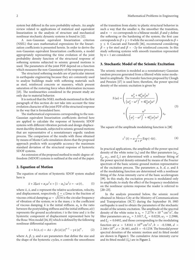
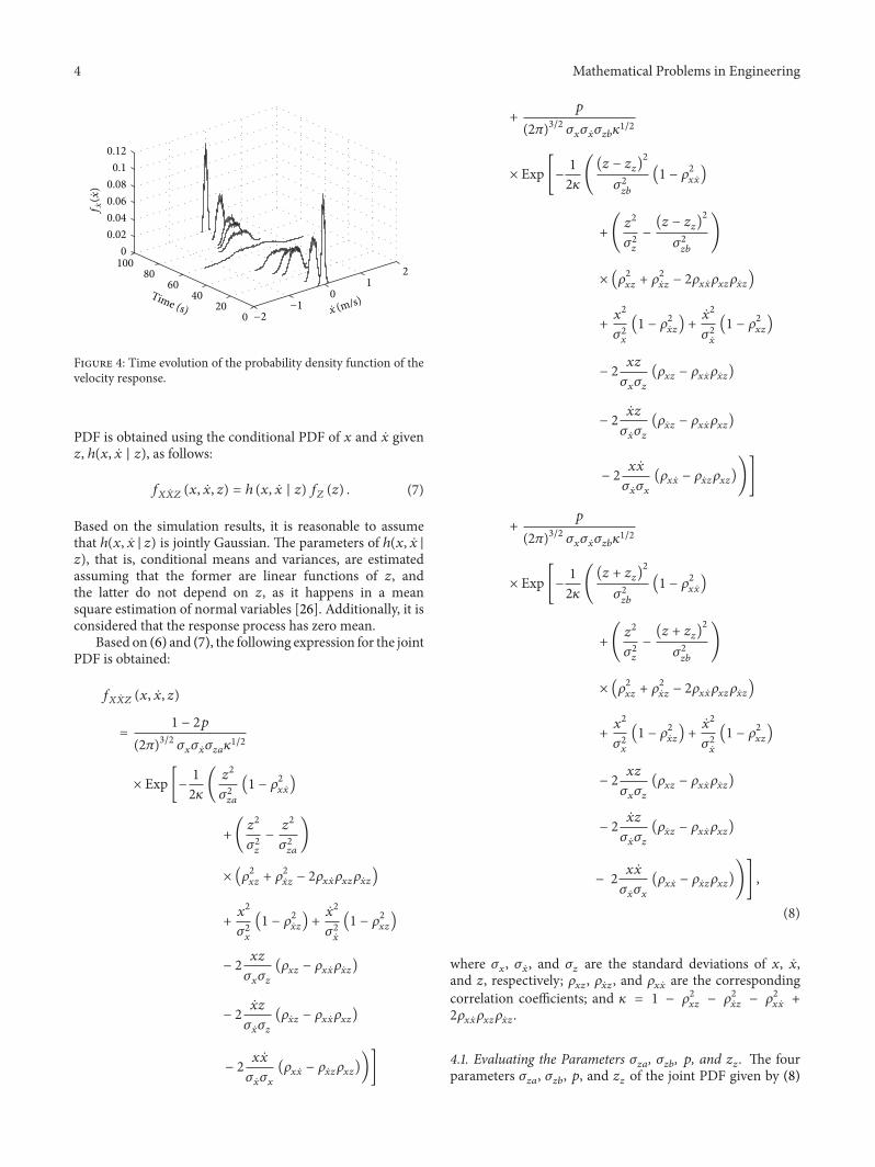
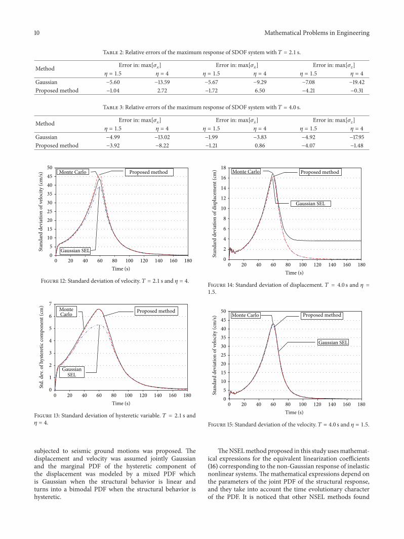
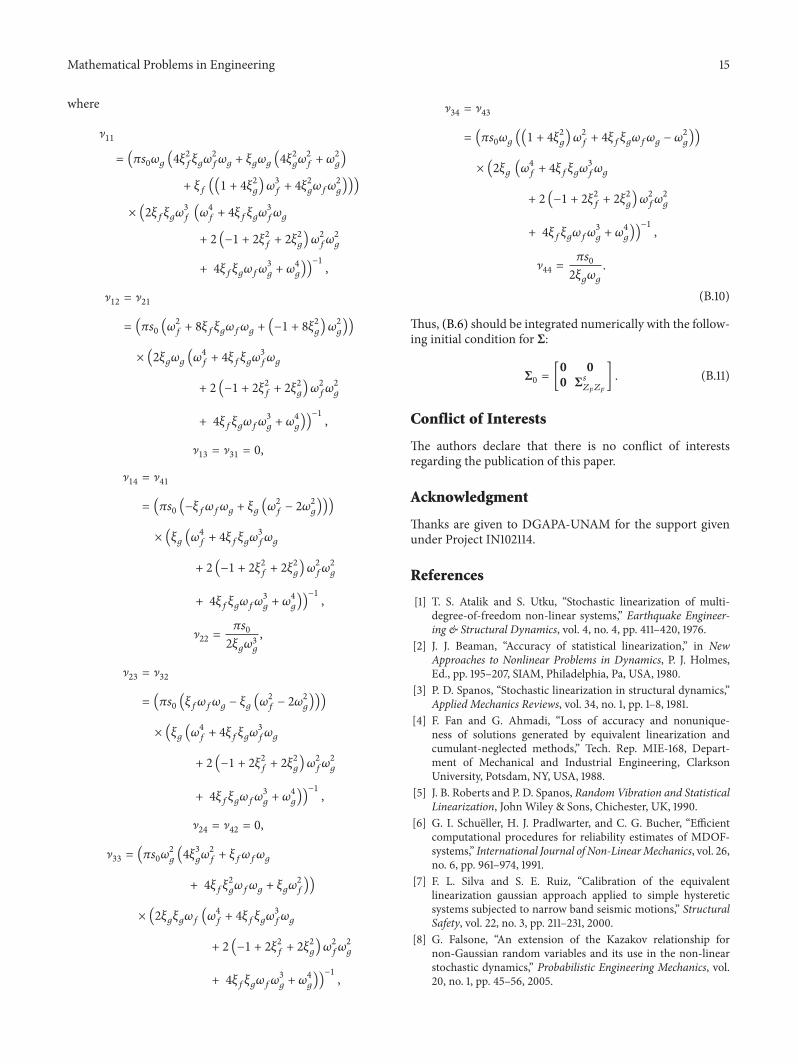system but differed in the zero probability subsets An amplereview related to applications of statistical and equivalentlinearization in the analysis of structure and mechanicalnonlinear stochastic dynamic systems is found in [12]

A non-Gaussian equivalent linearization criterion(NSEL) that uses mathematical expressions for the lineari-zation coefficients is presented herein In order to derive thenon-Gaussian equivalent linearization coefficients a modelappropriately representing the time evolution of the jointprobability density function of the structural response ofsoftening systems subjected to seismic ground motions isused The parameters of the joint PDF depend on a functionwhichmeasures the non-Gaussianity of the response process

The structural softening models are of particular interestin earthquake engineering because they are commonly usedto analyze buildings made with softening materials suchas steel reinforced concrete or masonry which presentsaturation of the restoring force when deformation increases[13] The nonlinearities considered in the present study areonly due to material behavior

It is noticed that theNSELmethodsmentioned in the firstparagraph of this section do not take into account the timeevolution character of the joint PDFof the structural responsein the way that is formulated here

Themathematical expressions corresponding to the non-Gaussian equivalent linearization coefficients derived hereare applied to calculate the response of hysteretic SDOFsystems with different vibration periods and design displace-ment ductility demands subjected to seismic groundmotionsthat are representative of a nonstationary ergodic randomprocess The comparison of the results with those obtainedbymeans ofMonte Carlo simulation shows that the proposedapproach predicts with acceptable accuracy the maximumstandard deviation of the structural response of hystereticSDOF systems

An extension of the proposedmethod tomulti-degree-of-freedom (MDOF) systems is outlined at the end of the paper

2 Equation of Motion

The equation of motion of hysteretic SDOF system studiedhere is

+ 2120585120596 + 120572

2120596

2119909 + (1 minus 120572

2) 120596

2119911 = minus119886 (119905)

(1)

where and 119909 represent the relative acceleration velocityand displacement respectively 120585 = 1198882119898120596 is the fraction ofviscous critical damping 120596 =

radic119896119898 is the circular frequency

of vibration of the system 119898 is the mass 119888 is the coefficientof viscous damping 119896 is the initial stiffness 120572

2is the ratio

between the postyielding stiffness and the initial stiffness 119886(119905)represents the ground acceleration 119905 is the time and 119911 is thehysteretic component of displacement represented here bytheBouc-Wenmodel [14 15]which is defined by the followingnonlinear differential equation

= ℎ ( 119911) = 119860 minus 120573119911 || |119911|

119899minus1minus 120574 |119911|

119899 (2)

where 119860 120573 120574 and 119899 are parameters that define the size andthe shape of the hysteretic cycles 119899 controls the smoothness

of the transition from elastic to plastic structural behavior insuch a way that the smaller 119899 the smoother the transitionand 119899 rarr infin corresponds to a bilinear model 120573 and 120574 definethe softening or the hardening of the system the first casecorresponds to120573 + 120574 gt 0while the second corresponds to120573 +

120574 le 0 Casciati and Faravelli [16] recommend considering120573 = 120574 for steel and 120573 = minus2120574 for reinforced concrete In thisstudy softening systems with smooth transition representedby 119899 = 1 are considered

3 Stochastic Model of the Seismic Excitation

The seismic motion is modeled as a nonstationary Gaussianrandom process generated from a filtered white noise modu-lated in amplitudeThe transfer function proposed by Cloughand Penzien [17] is used here therefore the power spectraldensity of the seismic excitation is given by

119878 (120596) = (

120596

4

119892+ 4120585

2

119892120596

2

119892120596

2

(120596

2

119892minus 120596

2)

2

+ 4120585

2

119892120596

2

119892120596

2

)

times(

120596

4

(120596

2

119891minus 120596

2)

2

+ 4120585

2

119891120596

2

119891120596

2

)119904

0

(3)

The square of the amplitude modulating function is [18]

119888

2(119905) = 119886

119905

119887

119889 + 119905

119890Exp (minus119896119905) (4)

In practical applications the amplitude of the power spectraldensity of the white noise (119904

0) and the filter parameters (120596

119892

120585

119892 120596119891 and 120585

119891) are determined with a nonlinear fitting of

the power spectral density estimated by means of the Fourierspectrum of the basic seismic ground motion representativeof the excitation process The parameters 119886 119887 119889 119890 and 119896

of the modulating function are determined with a nonlinearfitting of the Arias intensity curve of the basic accelerogram[19] In this study the excitation process is modulated onlyin amplitude to study the effect of the frequency modulationon the nonlinear systems response the reader is referred to[20ndash23]

In the analysis presented below the seismic recordobtained in Mexico City at the Ministry of Communicationsand Transportation (SCT) during the September 19 1985earthquake is used to obtain the parameters of the stochasticmodel of the seismic excitationThe amplitude of the spectraldensity of the white noise is 119904

0= 72776 times 10

minus4 cm2s3 thefilter parameters are 120596

119892= 31017 120585

119892= 00220 120596

119891= 22988

and 120585119891= 00492 and those corresponding to the modulating

function are 119886 = 58161 times 10

48 cm2s4 119887 = minus03388 119889 =

2166times10

47 119890 = 26461 and 119896 = minus01258The bimodal powerspectral densities of the seismic motion and its fitted modelare shown in Figure 1 The cumulative Arias intensity curveand its fitted model (119868

0) are in Figure 2



0

1000

2000

3000

4000

5000

6000

7000

8000

0 1 2 3 4 5

S(120596

) (cm

2s3)



0

20000

40000

60000

80000

100000

120000

140000

160000

0 20 40 60 80 100 120 140 160

intc2(t)dtI 0

(t) (

cm2s3)

Time t (s)

I0(t)intc2(t)dt


ing fitted model



119883(119909) and



119885(119911)




minus1minus05

005

1

0

005

01

015

02

025

03

x (m)Time (s)0

2040

6080

100

fx

(x)





119906


119906 Figure 5





119906le 119911 le 119911



119911

119906= (

119860

120573 + 120574

)

1119899

(5)




119891

119885(119911) =

119886120593

119885(119911) (1 minus 2119901) +

119887120593

119885(119911 minus 119911

119911) 119901

+

119887120593

119885(119911 + 119911

119911) 119901 0 le 119901 le 05

(6)

where119886120593



119911119886119887120593


with mean 119911

119911(or minus119911


119911119887 and 119901 is a


119887120593





119885

and119887120593








119891

119883119885(119909 119911) = ℎ (119909 | 119911) 119891

119885(119911) (7)



119891

119883119885(119909 119911)

=

1 minus 2119901

(2120587)

32120590

119909120590

119909120590

119911119886120581

12

times Exp[minus 1

2120581

(

119911

2

120590

2

119911119886

(1 minus 120588

2

119909 119909)

+ (

119911

2

120590

2

119911

minus

119911

2

120590

2

119911119886

)

times (120588

2

119909119911+ 120588

2

119909119911minus 2120588

119909 119909120588

119909119911120588

119909119911)

+

119909

2

120590

2

119909

(1 minus 120588

2

119909119911) +

2

120590

2

119909

(1 minus 120588

2

119909119911)

minus 2

119909119911

120590

119909120590

119911

(120588

119909119911minus 120588

119909120588

119909119911)

minus 2

119911

120590

119909120590

119911

(120588

119909119911minus 120588

119909120588

119909119911)

minus 2

119909

120590

119909120590

119909

(120588

119909 119909minus 120588

119909119911120588

119909119911))]

+

119901

(2120587)

32120590

119909120590

119909120590

119911119887120581

12

times Exp[minus 1

2120581

(

(119911 minus 119911

119911)

2

120590

2

119911119887

(1 minus 120588

2

119909 119909)

+ (

119911

2

120590

2

119911

minus

(119911 minus 119911

119911)

2

120590

2

119911119887

)

times (120588

2

119909119911+ 120588

2

119909119911minus 2120588

119909 119909120588

119909119911120588

119909119911)

+

119909

2

120590

2

119909

(1 minus 120588

2

119909119911) +

2

120590

2

119909

(1 minus 120588

2

119909119911)

minus 2

119909119911

120590

119909120590

119911

(120588

119909119911minus 120588

119909 119909120588

119909119911)

minus 2

119911

120590

119909120590

119911

(120588

119909119911minus 120588

119909 119909120588

119909119911)

minus 2

119909

120590

119909120590

119909

(120588

119909 119909minus 120588

119909119911120588

119909119911))]

+

119901

(2120587)

32120590

119909120590

119909120590

119911119887120581

12

times Exp[minus 1

2120581

(

(119911 + 119911

119911)

2

120590

2

119911119887

(1 minus 120588

2

119909 119909)

+ (

119911

2

120590

2

119911

minus

(119911 + 119911

119911)

2

120590

2

119911119887

)

times (120588

2

119909119911+ 120588

2

119909119911minus 2120588

119909 119909120588

119909119911120588

119909119911)

+

119909

2

120590

2

119909

(1 minus 120588

2

119909119911) +

2

120590

2

119909

(1 minus 120588

2

119909119911)

minus 2

119909119911

120590

119909120590

119911

(120588

119909119911minus 120588

119909 119909120588

119909119911)

minus 2

119911

120590

119909120590

119911

(120588

119909119911minus 120588

119909 119909120588

119909119911)

minus 2

119909

120590

119909120590

119909

(120588

119909 119909minus 120588

119909119911120588

119909119911))]

(8)

where 120590

119909 120590119909 and 120590





2

119909119911minus 120588

2

119909119911minus 120588

2

119909 119909+

2120588

119909 119909120588

119909119911120588

119909119911


119911 The four

parameters 120590119911119886 120590119911119887 119901 and 119911



020

4060

80100

minus01minus005

0005

01

0

02

04

06

08


+zu

fz(z

)



int

119911119906

minus119911119906

119891

119885(119911) 119889119911 = (1 minus 2119901)Erf(

119911

119911

radic2120590

119911119886

)

+ 119901[Erf(119911

119906minus 119911

119911

radic2120590

119911119887

)

+ Erf(119911

119906+ 119911

119911

radic2120590

119911119887

)] asymp 1

(9)


Erf (119906) = 2

radic120587

int

119906

0

Exp (minus1199052) 119889119905 (10)



as

119864 [119911

2] = ∭

infin

minusinfin

119911

2119891

119883119885(119909 119911) 119889119909 119889 119889119911

= int

infin

minusinfin

119911

2119891

119885(119911) 119889119911 = (1 minus 2119901) 120590

2

119911119886

+ 2119901 (119911

2

119911+ 120590

2

119911119887) = 120590

2

119911

(11)




120582 (119905) = int

minus119911119906

minusinfin

1

radic2120587120590

119911(119905)

Exp(minus 119911

2

2120590

2

119911(119905)

) 119889119911

=

1

2

(1 minus Erf(119911

119906

radic2120590

119911(119905)

))

(12)








119911119911

119911119906 120590119911119886120590

119911 120590119911119887120590

119911 and 119901 are

proposed

119911

119911(119905)

119911

119906

= 119886

1Ln (1198862120582 (119905) + 119886

3) + 119886

4

119901 (119905) = 119887

1Ln (1198872120582 (119905) + 119887

3) + 119887

4

120590

119911119886(119905)

120590

119911(119905)

= 119888

1Ln (1198882120582 (119905) + 119888

3) + 119888

4

120590

119911119887(119905)

120590

119911(119905)

= 119889

1Ln (1198892120582 (119905) + 119889

3) + 119889

4

(13)

where 119886

119894 119887119894 119888119894 and 119889



119911and 119901


119887120593

119885



119887120593




119885120590

119911and

119887120593

119885120590


119911


119911119886 120590119911119887 119901 and

119911



119885(119911) given by (6)


119894

119887

119894 119888119894 and 119889




01 and that 120590119911119886

gt 120590




minus01

01

03

05

07

09

000 002 004 006 008

120582

zz

zu

12

c3

c4

c5

c6

(a) 119911119911119911119906 versus 120582

000 002 004 006 008

120582

045

035

025

015

005

minus005

p

12

c6

c5c4c3

(b) 119901 versus 120582

120582

000 002 004 006 008

11

10

09

08

07

06

05

04

120590za120590z

12

c6

c5

c4

c3

(c) 120590119911119886120590119911 versus 120582

minus01

01

03

05

07

09

120582

000 002 004 006 008

120590zb120590z

12

c6

c5

c4c3

(d) 120590119911119887120590119911 versus 120582


119911119906 119901 120590119911119886120590

119911 and 120590

119911119887120590

119911versus 120582


minus2 0 2 4 6 8 10

020

4060

80100

120140

1601800

0102030405

z (cm)

Time (s)

fz(z

)






119886

1119886

2119886

3119886

4

0187 31990 0042 0590119887

1119887

2119887

3119887

4

0043 455126 0003 0240119888

1119888

2119888

3119888

4

minus0269 8247 0125 0442119889

1119889

2119889

3119889

4

minus0239 1408 0007 minus0391



= 119904

119890119909 + 119888

119890 + 119896

119890119911 (14)

where 119904119890 119888119890 and 119896



119867

119890= 119864 [119876119876

119879]

minus1

119864 [ℎ119876] (15)



119879 119867119890is the


[119904119890119888

119890119896

119890]



119904

119890= 0

119888

119890= (1 minus 2119901)119860 minus

radic

2

120587

120573

120588

119909119911120590

2

119911119886

radic120576

119886

minus

radic

2

120587

120574120590

119911119886

+ 2119901119860 minus 120573

radic

2

120587

120588

119909119911120590

2

119911119887

radic120576

119887

Exp(minus119911

2

119911120588

2

119909119911

2120576

119887

)

+119911

119911Erf(

119911

119911120588

119909119911

radic2120576

119887

)

minus 120574

radic

2

120587

120590

119911119887Exp(minus

119911

2

119911

2120590

2

119911119887

)

+ 119911

119911Erf(

119911

119911

radic2120590

119911119887

)

119896

119890= (1 minus 2119901)119860

120588

119909119911120590

119909(120590

2

119911119886minus 120590

2

119911)

120590

3

119911

minus

radic

2

120587

120573

120590

119909120590

2

119911119886

120590

3

119911

(120576

119886+ 120588

2

119909119911(120590

2

119911119886minus 120590

2

119911))

radic120576

119886

minus

radic

2

120587

120574

120588

119909119911120590

119909120590

119911119886(2120590

2

119911119886minus 120590

2

119911)

120590

3

119911

+ 2119901119860

120588

119909119911120590

119909(119911

2

119911+ 120590

2

119911119887minus 120590

2

119911)

120590

3

119911

minus 120573

120590

119909

120590

3

119911

times

radic

2

120587

Exp(minus119911

2

119911120588

2

119909119911

2120576

119887

)

times

119911

2

119911120576

119887+ 120590

2

119911119887(120576

119887+ 120588

2

119909119911(120590

2

119911119887minus120590

2

119911))

radic120576

119887

+ 119911

119911120588

119909119911(119911

2

119911+3120590

2

119911119887minus120590

2

119911)Erf(

119911

119911120588

119911

radic2120576

119887

)

+ 120574

120588

119909119911120590

119909

120590

3

119911

times

radic

2

120587

Exp(minus119911

2

119911

2120590

2

119911119887

)120590

119911119887(119911

2

119911+ 2120590

2

119911119887minus 120590

2

119911)

+ 119911

119911(119911

2

119911+ 3120590

2

119911119887minus 120590

2

119911)Erf(

119911

119911

radic2120590

119911119887

)

(16)

where 120576

119886= (1 minus 120588

2

119909119911)120590

2

119911+ 120588

2

119909119911120590

2

119911119886and 120576

119887= (1 minus 120588

2

119909119911)120590

2

119911+

120588

2

119909119911120590

2

119911119887



119879] where 119906(119905) =

[119909 119911 119909

119891119909

119892

119891

119892]


119889Σ (119905)

119889119905

= 119867 (119905) Σ (119905) + Σ (119905)119867

119879(119905) + 2120587119878

119865

(17)


119867(119905) =

[

[

[

[

[

[

[

[

[

[

[

[

[

[

0 1 0 0 0 0 0

minus120572

2120596


2) 120596

2120596

2

119891119888 (119905) minus120596

2

119892119888 (119905) 2120585

119891120596

119891119888 (119905) minus2120585

119892120596

119892119888 (119905)

119904

119890119888

119890119896

1198900 0 0 0

0 0 0 0 0 1 0

0 0 0 0 0 0 1

0 0 0 minus120596

2

119891120596

2

119892minus2120585

119891120596

1198912120585

119892120596

119892

0 0 0 0 minus120596

2

1198920 minus2120585

119892120596

119892

]

]

]

]

]

]

]

]

]

]

]

]

]

]

(18)


0

5

10

15

20

25

30

0 20 40 60 80 100 120 140 160 180

Stan

dard

dev

iatio

n of

disp

lace

men

t (cm

)

Time (s)

Monte Carlo

Proposedmethod

Gaussian SEL


0

10

20

30

40

50

60

70

80

0 20 40 60 80 100 120 140 160 180

Stan

dard

dev

iatio

n of

vel

ocity

(cm

s)

Time (s)

Proposed method

Gaussian SEL

Monte Carlo


119878


119865(7 7)which






0

5

10

15

20

25

0 20 40 60 80 100 120 140 160 180

Std

dev

of h

yste

retic

com

pone

nt (c

m)

Time (s)

GaussianSEL



0 20 40 60 80 100 120 140 160 1800

2

4

6

8

10

12

14

16

18

Time (s)

Stan

dard

dev

iatio

n of

disp

lace

men

t (cm

)Monte Carlo

Gaussian SEL

Proposed method








119909 120590119909and 120590119911) is obtained

as follows

120576 () =


times 100 (19)





Φ (q (119905) q (119905) q (119905)) = P (119905) (20)


Meq (119905) + Ceq (119905) + Keq (119905) = P (119905) (21)


119879]




Q = [q q q]119879 He = [MeCeKe]119879 (23)


He = 119864 [QQ119879]minus1

119864 [QΦ

119879(Q)]

(24)


119889Z (119905)

119889119905

= AeZ (119905) + BZF (119905) (25)


Ae (119905) = [


] (26)


119889ZF (119905)

119889119905

= DZF (119905) +W1015840 (119905) (27)


1015840


119889u119889119905

= H (119905) u +W(28)

where

u (119905) =

Z (119905)

ZF (119905) (29)

H (119905) = [

A B0 D] (30)



119889Σ (119905)

119889119905

= H (119905)Σ (119905) + Σ (119905)H119879 (119905) + 2120587SF (31)






9 Conclusions





119909] Error in max[120590

119911]

120578 = 15 120578 = 4 120578 = 15 120578 = 4 120578 = 15 120578 = 4




119909] Error in max[120590

119911]

120578 = 15 120578 = 4 120578 = 15 120578 = 4 120578 = 15 120578 = 4


0 20 40 60 80 100 120 140 160 1800

5

10

15

20

25

30

35

40

45

50

Time (s)

Stan

dard

dev

iatio

n of

vel

ocity

(cm

s) Monte Carlo

Gaussian SEL

Proposed method


7

6

5

4

3

2

1

00 20 40 60 80 100 120 140 160 180

Time (s)

Std

dev

of h

yste

retic

com

pone

nt (c

m)


GaussianSEL



0 20 40 60 80 100 120 140 160 1800

2

4

6

8

10

12

14

16

18

Time (s)

Stan

dard

dev

iatio

n of

disp

lace

men

t (cm

) Monte Carlo

Gaussian SEL

Proposed method


15

0 20 40 60 80 100 120 140 160 1800

5

10

15

20

25

30

35

40

45

50

Time (s)

Stan

dard

dev

iatio

n of

vel

ocity

(cm

s) Monte Carlo

Gaussian SEL

Proposed method




0 20 40 60 80 100 120 140 160 180

Time (s)

14

12

10

8

6

4

2

0

Std

dev

of h

yste

retic

com

pone

nt (c


Gaussian SEL


0 20 40 60 80 100 120 140 160 1800

2

4

6

8

10

12

14

16

Time (s)

Stan

dard

dev

iatio

n of

disp

lace

men

t (cm

) Monte Carlo

Gaussian SEL

Proposed method


40





0 20 40 60 80 100 120 140 160 1800

5

10

15

20

25

30

35

40

Time (s)

Stan

dard

dev

iatio

n of

vel

ocity

(cm

s)

Monte Carlo

Gaussian SEL

Proposed method


0 20 40 60 80 100 120 140 160 180

Time (s)

7

6

5

4

3

2

1

0

Std

dev

of h

yste

retic

com

pone

nt (c

m)

Proposed method

Monte Carlo

Gaussian SEL




119894 119894 = 1 2 3 4 in (13) can be


Appendices




119867

119890= 119864 [119876119876

119879]

minus1

119864 [ℎ119876] (A1)




119879 and 119867

119890=

[119904119890119888

119890119896

119890]

119879



Σ

minus1

119876=

1

120590

2

119909120590

2

119909120590

2

119911120581

[

[

[

[

(1 minus 120588

2

119909119911) 120590

2

119909120590

2

119911(120588

119909119911120588

119909119911minus 120588

119909 119909) 120590

119909120590

119909120590

2

119911(120588

119909119911120588

119909 119909minus 120588

119909119911) 120590

2

119909120590

119909120590

119911

(120588

119909119911120588

119909119911minus 120588

119909) 120590

119909120590

119909120590

2

119911(1 minus 120588

2

119909119911) 120590

2

119909120590

2

119911(120588

119909 119909120588

119909119911minus 120588

119909119911) 120590

119909120590

2

119909120590

119911

(120588

119909119911120588

119909minus 120588

119909119911) 120590

2

119909120590

119909120590

119911(120588

119909 119909120588

119909119911minus 120588

119911) 120590

119909120590

2

119909120590

119911(1 minus 120588

2

119909 119909) 120590

2

119909120590

2

119911

]

]

]

]

(A2)

where 120581 = 1minus120588

2

119909119911minus120588

2

119909119911minus120588

2

119909 119909+2120588

119909 119909120588

119909119911120588



119864 [ℎ119876] =

[

[

[

119864 [119909ℎ ( 119911)]

119864 [ℎ ( 119911)]

119864 [119911ℎ ( 119911)]

]

]

]

=

[

[

[

119860119865

1minus 120573119865

2minus 120574119865

3

119860119865

4minus 120573119865

5minus 120574119865

6

119860119865

7minus 120573119865

8minus 120574119865

9

]

]

]

(A3)

where

119865

1= 119864 [119909] = ∬

infin

minusinfin

119909119891

119883119889119909 119889

119865

2= 119864 [119909119911 || |119911|

119899minus1]

= ∭

infin

minusinfin

119909119911 || |119911|

119899minus1119891

119883119885119889119909 119889 119889119911

119865

3= 119864 [119909 |119911|

119899] = ∭

infin

minusinfin

119909 |119911|

119899119891

119883119885119889119909 119889 119889119911

119865

4= 119864 [

2] = int

infin

minusinfin

2119891

119889

119865

5= 119864 [119911 || |119911|

119899minus1] = ∬

infin

minusinfin

119911 || |119911|

119899minus1119891

119885119889 119889119911

119865

6= 119864 [

2|119911|

119899] = ∬

infin

minusinfin

2|119911|

119899119891

119885119889 119889119911

119865

7= 119864 [119911] = ∬

infin

minusinfin

119911119891

119885119889119889119911

119865

8= 119864 [119911

2|| |119911|

119899minus1] = ∬

infin

minusinfin

119911

2|| |119911|

119899minus1119891

119885119889 119889119911

119865

9= 119864 [119911 |119911|

119899] = ∬

infin

minusinfin

119911 |119911|

119899119891

119885119889 119889119911

(A4)


is modeled by (8) 119891119885

119891119883

and119891



119865

1= (1 minus 2119901) 119865

1119886+ 2119901119865

1119887

119865

2= (1 minus 2119901) 119865

2119886+ 2119901119865

2119887

119865

3= (1 minus 2119901) 119865

3119886+ 2119901119865

3119887

119865

4= (1 minus 2119901) 119865

4119886+ 2119901119865

4119887

119865

5= (1 minus 2119901) 119865

5119886+ 2119901119865

5119887

119865

6= (1 minus 2119901) 119865

6119886+ 2119901119865

6119887

119865

7= (1 minus 2119901) 119865

7119886+ 2119901119865

7119887

119865

8= (1 minus 2119901) 119865

8119886+ 2119901119865

8119887

119865

9= (1 minus 2119901) 119865

9119886+ 2119901119865

9119887

(A5)

where

119865

1119886=

120590

119909120590

119909

120590

2

119911

[120590

2

119911(120588

119909minus 120588

119909119911120588

119909119911) + 120588

119909119911120588

119909119911120590

2

119911119886]

119865

1119887=

120590

119909120590

119909

120590

2

119911

[120590

2

119911(120588

119909 119909minus 120588

119909119911120588

119909119911) + 120588

119909119911120588

119909119911(119911

2

119911+ 120590

2

119911119887)]

119865

2119886=

radic

2

120587

120590

119909120590

119909120590

2

119911119886

120590

2

119911radic120576

119886

[120588

119909119911120576

119886

+ 120588

119909119911120590

2

119911(120588

119909 119909minus 120588

119909119911120588

119909119911)

+ 120588

119909119911120588

119909119911120590

2

119911119886]

119865

2119887

=

120590

119909120590

119909

radic2120587120590

2

119911

[

2

radic120576

119887

Exp[minus119911

2

119911120588

2

119909119911

2120576

119887

]

times 120588

119909119911(119911

2

119911+ 120590

2

119911119887) 120576

119887

+ 120590

2

119911119887120588

119909119911(120590

2

119911(120588

119909 119909minus 120588

119909119911120588

119909119911)

+ 120588

119909119911120588

119909119911120590

2

119911119887)

+

radic

2120587119911

119911(120590

2

119911(120588

119909 119909minus 120588

119909119911120588

119909119911)

+ 120588

119909119911120588

119909119911(119911

2

119911+ 3120590

2

119911119887))

times Erf[119911

119911120588

119909119911

radic2120576

119887

]]

119865

3119886=

radic

2

120587

120590

119909120590

119909120590

119911119886

120590

2

119911

[120590

2

119911(120588

119909 119909minus 120588

119909119911120588

119909119911)

+ 2120588

119909119911120588

119909119911120590

2

119911119886]


119865

3119887

=

120590

119909120590

119909

radic2120587120590

2

119911

[2120590

119911119887Exp[minus

119911

2

119911

2120590

2

119911119887

]

times [120590

2

119911(120588

119909minus 120588

119909119911120588

119909119911)

+ 120588

119909119911120588

119909119911(119911

2

119911+ 2120590

2

119911119887)]

+

radic

2120587119911

119911Erf[

119911

119911

radic2120590

119911119887

]

times [120590

2

119911(120588

119909minus 120588

119909119911120588

119909119911)

+ 120588

119909119911120588

119909119911(119911

2

119911+ 3120590

2

119911119887)]]

119865

4119886=

120590

2

119909

120590

2

119911

120576

119886

119865

4119887=

120590

2

119909

120590

2

119911

(120576

119887+ 120588

2

119909119911119911

2

119911)

119865

5119886=

radic

8

120587

120590

2

119909120590

2

119911119886

120590

2

119911

120588

119909119911radic120576

119886

119865

5119887

=

120590

2

119909

radic2120587120590

2

119911

[2120588

119909119911(119911

2

119911+ 2120590

2

119911119887)radic120576

119887Exp[minus

119911

2

119911120588

2

119909119911

2120576

119887

]

+

radic

2120587119911

119911120576

119887+ 120588

2

119909119911(119911

2

119911+ 2120590

2

119911119887)

times Erf[119911

119911120588

119909119911

radic2120576

119887

]]

119865

6119886=

radic

2

120587

120590

2

119909120590

119911119886

120590

2

119911

(120576

119886+ 120588

2

119909119911120590

2

119911119886)

119865

6119887

=

120590

2

119909

radic2120587120590

2

119911

[2120590

119911119887Exp[minus

119911

2

119911

2120590

2

119911119887

] 120576

119887+ 120588

2

119909119911(119911

2

119911+ 120590

2

119911119887)

+

radic

2120587119911

119911120576

119887+ 120588

2

119909119911(119911

2

119911+ 2120590

2

119911119887)

times Erf[119911

119911

radic2120590

119911119887

]]

119865

7119886=

120590

119909120588

119909119911120590

2

119911119886

120590

119911

119865

7119887=

120590

119909120588

119909119911

120590

119911

(119911

2

119911+ 120590

2

119911119887)

119865

8119886=

radic

2

120587

120590

119909120590

2

119911119886

120590

119911radic120576

119886

(120576

119886+ 120590

2

119911119886120588

2

119909119911)

119865

8119887

=

120590

119909

radic2120587120590

119911

[

2

radic120576

119887

Exp[minus119911

2

119911120588

2

119909119911

2120576

119887

] 120576

119887(119911

2

119911+ 120590

2

119911119887) + 120590

4

119911119887120588

2

119909119911

+

radic

2120587119911

119911120588

119909119911(119911

2

119911+ 3120590

2

119911119887)Erf[

119911

119911120588

119909119911

radic2120576

119887

]]

119865

9119886=

radic

8

120587

120590

119909120590

3

119911119886120588

119911

120590

119911

119865

9119887

=

120590

119909120588

119909119911

radic2120587120590

119911

[2120590

119911119887(119911

2

119911+ 2120590

2

119911119887)Exp[minus

119911

2

119911

2120590

2

119911119887

]

+

radic

2120587119911

119911(119911

2

119911+ 3120590

2

119911119887)Erf[

119911

119911

radic2120590

119911119887

]]

(A6)

where 120576119886= (1minus120588

2

119909119911)120590

2

119911+120588

2

119909119911120590

2

119911119886 120576119887= (1minus120588

2

119909119911)120590

2

119911+120588

2

119909119911120590

2

119911119887 Exp[sdot]


Erf [119906] = 2

radic120587

int

119906

0

Exp [minus1199052] 119889119905 (A7)


119904

119890= 0

119888

119890= (1 minus 2119901)

times [119860 minus

radic

2

120587

120573

120588

119909119911120590

2

119911119886

radic120576

119886

minus

radic

2

120587

120574120590

119911119886]

+ 2119901[119860 minus 120573

times

radic

2

120587

120588

119909119911120590

2

119911119887

radic120576

119887

Exp(minus119911

2

119911120588

2

119909119911

2120576

119887

)

+ 119911

119911Erf(

119911

119911120588

119909119911

radic2120576

119887

)

minus 120574

radic

2

120587

120590

119911119887Exp(minus

119911

2

119911

2120590

2

119911119887

)

+ 119911

119911Erf(

119911

119911

radic2120590

119911119887

)]

119896

119890= (1 minus 2119901) [119860

120588

119909119911120590

119909(120590

2

119911119886minus 120590

2

119911)

120590

3

119911

minus

radic

2

120587

120573

120590

119909120590

2

119911119886

120590

3

119911

(120576

119886+ 120588

2

119909119911(120590

2

119911119886minus 120590

2

119911))

radic120576

119886

minus

radic

2

120587

120574

120588

119909119911120590

119909120590

119911119886(2120590

2

119911119886minus 120590

2

119911)

120590

3

119911

]


+ 2119901[119860

120588

119909119911120590

119909(119911

2

119911+ 120590

2

119911119887minus 120590

2

119911)

120590

3

119911

minus 120573

120590

119909

120590

3

119911

times

radic

2

120587

Exp(minus119911

2

119911120588

2

119909119911

2120576

119887

)

times

119911

2

119911120576

119887+ 120590

2

119911119887(120576

119887+ 120588

2

119909119911(120590

2

119911119887minus 120590

2

119911))

radic120576

119887

+ 119911

119911120588

119909119911(119911

2

119911+ 3120590

2

119911119887minus 120590

2

119911)

times Erf(119911

119911120588

119909119911

radic2120576

119887

)

minus 120574

120588

119909119911120590

119909

120590

3

119911

radic

2

120587

Exp(minus119911

2

119911

2120590

2

119911119887

)

times 120590

119911119887(119911

2

119911+ 2120590

2

119911119887minus 120590

2

119911)

+ 119911

119911(119911

2

119911+ 3120590

2

119911119887minus 120590

2

119911)

times Erf(119911

119911

radic2120590

119911119887

)]

(A8)



119889Z (119905)

119889119905

= AZ (119905) + BZF (119905) (B1)


119889ZF (119905)

119889119905

= DZF (119905) +W1015840 (119905) (B2)



119889u119889119905

= H (119905) u +W(B3)

where

u (119905) =

Z (119905)

ZF (119905) (B4)

H (119905) = [

A B0 D

] (B5)



119889Σ (119905)

119889119905

= H (119905)Σ (119905) + Σ (119905)H119879 (119905) + 2120587SF (B6)


0)


Σ = [

Σ119885119885Σ119885119885119865

Σ119879

119885119885119865

Σ119885119865119885119865

] (B7)

where Σ119885119885

= 119864[ZZ119879] Σ119885119885119865

= 119864[ZZ119879F ] and Σ119885119865119885119865 =


119885119885and Σ

119885119885119865



DΣ119904119885119865119885119865

+ Σ119904

119885119865119885119865

D119879 + P1015840 = 0 (B8)


Σ119904

119885119865119885119865

=

[

[

[

[

[

[

]11

]12

]13

]14

]21

]22

]23

]24

]31

]32

]33

]34

]41

]42

]43

]44

]

]

]

]

]

]

(B9)


where

]11

= (120587119904

0120596

119892(4120585

2

119891120585

119892120596

2

119891120596

119892+ 120585

119892120596

119892(4120585

2

119892120596

2

119891+ 120596

2

119892)

+ 120585

119891((1 + 4120585

2

119892) 120596

3

119891+ 4120585

2

119892120596

119891120596

2

119892)))

times (2120585

119891120585

119892120596

3

119891(120596

4

119891+ 4120585

119891120585

119892120596

3

119891120596

119892

+ 2 (minus1 + 2120585

2

119891+ 2120585

2

119892) 120596

2

119891120596

2

119892

+ 4120585

119891120585

119892120596

119891120596

3

119892+ 120596

4

119892))

minus1

]12

= ]21

= (120587119904

0(120596

2

119891+ 8120585

119891120585

119892120596

119891120596

119892+ (minus1 + 8120585

2

119892) 120596

2

119892))

times (2120585

119892120596

119892(120596

4

119891+ 4120585

119891120585

119892120596

3

119891120596

119892

+ 2 (minus1 + 2120585

2

119891+ 2120585

2

119892) 120596

2

119891120596

2

119892

+ 4120585

119891120585

119892120596

119891120596

3

119892+ 120596

4

119892))

minus1

]13

= ]31

= 0

]14

= ]41

= (120587119904

0(minus120585

119891120596

119891120596

119892+ 120585

119892(120596

2

119891minus 2120596

2

119892)))

times (120585

119892(120596

4

119891+ 4120585

119891120585

119892120596

3

119891120596

119892

+ 2 (minus1 + 2120585

2

119891+ 2120585

2

119892) 120596

2

119891120596

2

119892

+ 4120585

119891120585

119892120596

119891120596

3

119892+ 120596

4

119892))

minus1

]22

=

120587119904

0

2120585

119892120596

3

119892

]23

= ]32

= (120587119904

0(120585

119891120596

119891120596

119892minus 120585

119892(120596

2

119891minus 2120596

2

119892)))

times (120585

119892(120596

4

119891+ 4120585

119891120585

119892120596

3

119891120596

119892

+ 2 (minus1 + 2120585

2

119891+ 2120585

2

119892) 120596

2

119891120596

2

119892

+ 4120585

119891120585

119892120596

119891120596

3

119892+ 120596

4

119892))

minus1

]24

= ]42

= 0

]33

= (120587119904

0120596

2

119892(4120585

3

119892120596

2

119891+ 120585

119891120596

119891120596

119892

+ 4120585

119891120585

2

119892120596

119891120596

119892+ 120585

119892120596

2

119891))

times (2120585

119892120585

119892120596

119891(120596

4

119891+ 4120585

119891120585

119892120596

3

119891120596

119892

+ 2 (minus1 + 2120585

2

119891+ 2120585

2

119892) 120596

2

119891120596

2

119892

+ 4120585

119891120585

119892120596

119891120596

3

119892+ 120596

4

119892))

minus1

]34

= ]43

= (120587119904

0120596

119892((1 + 4120585

2

119892) 120596

2

119891+ 4120585

119891120585

119892120596

119891120596

119892minus 120596

2

119892))

times (2120585

119892(120596

4

119891+ 4120585

119891120585

119892120596

3

119891120596

119892

+ 2 (minus1 + 2120585

2

119891+ 2120585

2

119892) 120596

2

119891120596

2

119892

+ 4120585

119891120585

119892120596

119891120596

3

119892+ 120596

4

119892))

minus1

]44

=

120587119904

0

2120585

119892120596

119892

(B10)


Σ0= [

0 00 Σ119904119885119865119885119865

] (B11)



Acknowledgment


References







































Volume 2014




Journal of











Journal of


Function Spaces






Algebra











0

1000

2000

3000

4000

5000

6000

7000

8000

0 1 2 3 4 5

S(120596

) (cm

2s3)



0

20000

40000

60000

80000

100000

120000

140000

160000

0 20 40 60 80 100 120 140 160

intc2(t)dtI 0

(t) (

cm2s3)

Time t (s)

I0(t)intc2(t)dt


ing fitted model



119883(119909) and



119885(119911)




minus1minus05

005

1

0

005

01

015

02

025

03

x (m)Time (s)0

2040

6080

100

fx

(x)





119906


119906 Figure 5





119906le 119911 le 119911



119911

119906= (

119860

120573 + 120574

)

1119899

(5)




119891

119885(119911) =

119886120593

119885(119911) (1 minus 2119901) +

119887120593

119885(119911 minus 119911

119911) 119901

+

119887120593

119885(119911 + 119911

119911) 119901 0 le 119901 le 05

(6)

where119886120593



119911119886119887120593


with mean 119911

119911(or minus119911


119911119887 and 119901 is a


119887120593





119885

and119887120593








119891

119883119885(119909 119911) = ℎ (119909 | 119911) 119891

119885(119911) (7)



119891

119883119885(119909 119911)

=

1 minus 2119901

(2120587)

32120590

119909120590

119909120590

119911119886120581

12

times Exp[minus 1

2120581

(

119911

2

120590

2

119911119886

(1 minus 120588

2

119909 119909)

+ (

119911

2

120590

2

119911

minus

119911

2

120590

2

119911119886

)

times (120588

2

119909119911+ 120588

2

119909119911minus 2120588

119909 119909120588

119909119911120588

119909119911)

+

119909

2

120590

2

119909

(1 minus 120588

2

119909119911) +

2

120590

2

119909

(1 minus 120588

2

119909119911)

minus 2

119909119911

120590

119909120590

119911

(120588

119909119911minus 120588

119909120588

119909119911)

minus 2

119911

120590

119909120590

119911

(120588

119909119911minus 120588

119909120588

119909119911)

minus 2

119909

120590

119909120590

119909

(120588

119909 119909minus 120588

119909119911120588

119909119911))]

+

119901

(2120587)

32120590

119909120590

119909120590

119911119887120581

12

times Exp[minus 1

2120581

(

(119911 minus 119911

119911)

2

120590

2

119911119887

(1 minus 120588

2

119909 119909)

+ (

119911

2

120590

2

119911

minus

(119911 minus 119911

119911)

2

120590

2

119911119887

)

times (120588

2

119909119911+ 120588

2

119909119911minus 2120588

119909 119909120588

119909119911120588

119909119911)

+

119909

2

120590

2

119909

(1 minus 120588

2

119909119911) +

2

120590

2

119909

(1 minus 120588

2

119909119911)

minus 2

119909119911

120590

119909120590

119911

(120588

119909119911minus 120588

119909 119909120588

119909119911)

minus 2

119911

120590

119909120590

119911

(120588

119909119911minus 120588

119909 119909120588

119909119911)

minus 2

119909

120590

119909120590

119909

(120588

119909 119909minus 120588

119909119911120588

119909119911))]

+

119901

(2120587)

32120590

119909120590

119909120590

119911119887120581

12

times Exp[minus 1

2120581

(

(119911 + 119911

119911)

2

120590

2

119911119887

(1 minus 120588

2

119909 119909)

+ (

119911

2

120590

2

119911

minus

(119911 + 119911

119911)

2

120590

2

119911119887

)

times (120588

2

119909119911+ 120588

2

119909119911minus 2120588

119909 119909120588

119909119911120588

119909119911)

+

119909

2

120590

2

119909

(1 minus 120588

2

119909119911) +

2

120590

2

119909

(1 minus 120588

2

119909119911)

minus 2

119909119911

120590

119909120590

119911

(120588

119909119911minus 120588

119909 119909120588

119909119911)

minus 2

119911

120590

119909120590

119911

(120588

119909119911minus 120588

119909 119909120588

119909119911)

minus 2

119909

120590

119909120590

119909

(120588

119909 119909minus 120588

119909119911120588

119909119911))]

(8)

where 120590

119909 120590119909 and 120590





2

119909119911minus 120588

2

119909119911minus 120588

2

119909 119909+

2120588

119909 119909120588

119909119911120588

119909119911


119911 The four

parameters 120590119911119886 120590119911119887 119901 and 119911



020

4060

80100

minus01minus005

0005

01

0

02

04

06

08


+zu

fz(z

)



int

119911119906

minus119911119906

119891

119885(119911) 119889119911 = (1 minus 2119901)Erf(

119911

119911

radic2120590

119911119886

)

+ 119901[Erf(119911

119906minus 119911

119911

radic2120590

119911119887

)

+ Erf(119911

119906+ 119911

119911

radic2120590

119911119887

)] asymp 1

(9)


Erf (119906) = 2

radic120587

int

119906

0

Exp (minus1199052) 119889119905 (10)



as

119864 [119911

2] = ∭

infin

minusinfin

119911

2119891

119883119885(119909 119911) 119889119909 119889 119889119911

= int

infin

minusinfin

119911

2119891

119885(119911) 119889119911 = (1 minus 2119901) 120590

2

119911119886

+ 2119901 (119911

2

119911+ 120590

2

119911119887) = 120590

2

119911

(11)




120582 (119905) = int

minus119911119906

minusinfin

1

radic2120587120590

119911(119905)

Exp(minus 119911

2

2120590

2

119911(119905)

) 119889119911

=

1

2

(1 minus Erf(119911

119906

radic2120590

119911(119905)

))

(12)








119911119911

119911119906 120590119911119886120590

119911 120590119911119887120590

119911 and 119901 are

proposed

119911

119911(119905)

119911

119906

= 119886

1Ln (1198862120582 (119905) + 119886

3) + 119886

4

119901 (119905) = 119887

1Ln (1198872120582 (119905) + 119887

3) + 119887

4

120590

119911119886(119905)

120590

119911(119905)

= 119888

1Ln (1198882120582 (119905) + 119888

3) + 119888

4

120590

119911119887(119905)

120590

119911(119905)

= 119889

1Ln (1198892120582 (119905) + 119889

3) + 119889

4

(13)

where 119886

119894 119887119894 119888119894 and 119889



119911and 119901


119887120593

119885



119887120593




119885120590

119911and

119887120593

119885120590


119911


119911119886 120590119911119887 119901 and

119911



119885(119911) given by (6)


119894

119887

119894 119888119894 and 119889




01 and that 120590119911119886

gt 120590




minus01

01

03

05

07

09

000 002 004 006 008

120582

zz

zu

12

c3

c4

c5

c6

(a) 119911119911119911119906 versus 120582

000 002 004 006 008

120582

045

035

025

015

005

minus005

p

12

c6

c5c4c3

(b) 119901 versus 120582

120582

000 002 004 006 008

11

10

09

08

07

06

05

04

120590za120590z

12

c6

c5

c4

c3

(c) 120590119911119886120590119911 versus 120582

minus01

01

03

05

07

09

120582

000 002 004 006 008

120590zb120590z

12

c6

c5

c4c3

(d) 120590119911119887120590119911 versus 120582


119911119906 119901 120590119911119886120590

119911 and 120590

119911119887120590

119911versus 120582


minus2 0 2 4 6 8 10

020

4060

80100

120140

1601800

0102030405

z (cm)

Time (s)

fz(z

)






119886

1119886

2119886

3119886

4

0187 31990 0042 0590119887

1119887

2119887

3119887

4

0043 455126 0003 0240119888

1119888

2119888

3119888

4

minus0269 8247 0125 0442119889

1119889

2119889

3119889

4

minus0239 1408 0007 minus0391



= 119904

119890119909 + 119888

119890 + 119896

119890119911 (14)

where 119904119890 119888119890 and 119896



119867

119890= 119864 [119876119876

119879]

minus1

119864 [ℎ119876] (15)



119879 119867119890is the


[119904119890119888

119890119896

119890]



119904

119890= 0

119888

119890= (1 minus 2119901)119860 minus

radic

2

120587

120573

120588

119909119911120590

2

119911119886

radic120576

119886

minus

radic

2

120587

120574120590

119911119886

+ 2119901119860 minus 120573

radic

2

120587

120588

119909119911120590

2

119911119887

radic120576

119887

Exp(minus119911

2

119911120588

2

119909119911

2120576

119887

)

+119911

119911Erf(

119911

119911120588

119909119911

radic2120576

119887

)

minus 120574

radic

2

120587

120590

119911119887Exp(minus

119911

2

119911

2120590

2

119911119887

)

+ 119911

119911Erf(

119911

119911

radic2120590

119911119887

)

119896

119890= (1 minus 2119901)119860

120588

119909119911120590

119909(120590

2

119911119886minus 120590

2

119911)

120590

3

119911

minus

radic

2

120587

120573

120590

119909120590

2

119911119886

120590

3

119911

(120576

119886+ 120588

2

119909119911(120590

2

119911119886minus 120590

2

119911))

radic120576

119886

minus

radic

2

120587

120574

120588

119909119911120590

119909120590

119911119886(2120590

2

119911119886minus 120590

2

119911)

120590

3

119911

+ 2119901119860

120588

119909119911120590

119909(119911

2

119911+ 120590

2

119911119887minus 120590

2

119911)

120590

3

119911

minus 120573

120590

119909

120590

3

119911

times

radic

2

120587

Exp(minus119911

2

119911120588

2

119909119911

2120576

119887

)

times

119911

2

119911120576

119887+ 120590

2

119911119887(120576

119887+ 120588

2

119909119911(120590

2

119911119887minus120590

2

119911))

radic120576

119887

+ 119911

119911120588

119909119911(119911

2

119911+3120590

2

119911119887minus120590

2

119911)Erf(

119911

119911120588

119911

radic2120576

119887

)

+ 120574

120588

119909119911120590

119909

120590

3

119911

times

radic

2

120587

Exp(minus119911

2

119911

2120590

2

119911119887

)120590

119911119887(119911

2

119911+ 2120590

2

119911119887minus 120590

2

119911)

+ 119911

119911(119911

2

119911+ 3120590

2

119911119887minus 120590

2

119911)Erf(

119911

119911

radic2120590

119911119887

)

(16)

where 120576

119886= (1 minus 120588

2

119909119911)120590

2

119911+ 120588

2

119909119911120590

2

119911119886and 120576

119887= (1 minus 120588

2

119909119911)120590

2

119911+

120588

2

119909119911120590

2

119911119887



119879] where 119906(119905) =

[119909 119911 119909

119891119909

119892

119891

119892]


119889Σ (119905)

119889119905

= 119867 (119905) Σ (119905) + Σ (119905)119867

119879(119905) + 2120587119878

119865

(17)


119867(119905) =

[

[

[

[

[

[

[

[

[

[

[

[

[

[

0 1 0 0 0 0 0

minus120572

2120596


2) 120596

2120596

2

119891119888 (119905) minus120596

2

119892119888 (119905) 2120585

119891120596

119891119888 (119905) minus2120585

119892120596

119892119888 (119905)

119904

119890119888

119890119896

1198900 0 0 0

0 0 0 0 0 1 0

0 0 0 0 0 0 1

0 0 0 minus120596

2

119891120596

2

119892minus2120585

119891120596

1198912120585

119892120596

119892

0 0 0 0 minus120596

2

1198920 minus2120585

119892120596

119892

]

]

]

]

]

]

]

]

]

]

]

]

]

]

(18)


0

5

10

15

20

25

30

0 20 40 60 80 100 120 140 160 180

Stan

dard

dev

iatio

n of

disp

lace

men

t (cm

)

Time (s)

Monte Carlo

Proposedmethod

Gaussian SEL


0

10

20

30

40

50

60

70

80

0 20 40 60 80 100 120 140 160 180

Stan

dard

dev

iatio

n of

vel

ocity

(cm

s)

Time (s)

Proposed method

Gaussian SEL

Monte Carlo


119878


119865(7 7)which






0

5

10

15

20

25

0 20 40 60 80 100 120 140 160 180

Std

dev

of h

yste

retic

com

pone

nt (c

m)

Time (s)

GaussianSEL



0 20 40 60 80 100 120 140 160 1800

2

4

6

8

10

12

14

16

18

Time (s)

Stan

dard

dev

iatio

n of

disp

lace

men

t (cm

)Monte Carlo

Gaussian SEL

Proposed method








119909 120590119909and 120590119911) is obtained

as follows

120576 () =


times 100 (19)





Φ (q (119905) q (119905) q (119905)) = P (119905) (20)


Meq (119905) + Ceq (119905) + Keq (119905) = P (119905) (21)


119879]




Q = [q q q]119879 He = [MeCeKe]119879 (23)


He = 119864 [QQ119879]minus1

119864 [QΦ

119879(Q)]

(24)


119889Z (119905)

119889119905

= AeZ (119905) + BZF (119905) (25)


Ae (119905) = [


] (26)


119889ZF (119905)

119889119905

= DZF (119905) +W1015840 (119905) (27)


1015840


119889u119889119905

= H (119905) u +W(28)

where

u (119905) =

Z (119905)

ZF (119905) (29)

H (119905) = [

A B0 D] (30)



119889Σ (119905)

119889119905

= H (119905)Σ (119905) + Σ (119905)H119879 (119905) + 2120587SF (31)






9 Conclusions





119909] Error in max[120590

119911]

120578 = 15 120578 = 4 120578 = 15 120578 = 4 120578 = 15 120578 = 4




119909] Error in max[120590

119911]

120578 = 15 120578 = 4 120578 = 15 120578 = 4 120578 = 15 120578 = 4


0 20 40 60 80 100 120 140 160 1800

5

10

15

20

25

30

35

40

45

50

Time (s)

Stan

dard

dev

iatio

n of

vel

ocity

(cm

s) Monte Carlo

Gaussian SEL

Proposed method


7

6

5

4

3

2

1

00 20 40 60 80 100 120 140 160 180

Time (s)

Std

dev

of h

yste

retic

com

pone

nt (c

m)


GaussianSEL



0 20 40 60 80 100 120 140 160 1800

2

4

6

8

10

12

14

16

18

Time (s)

Stan

dard

dev

iatio

n of

disp

lace

men

t (cm

) Monte Carlo

Gaussian SEL

Proposed method


15

0 20 40 60 80 100 120 140 160 1800

5

10

15

20

25

30

35

40

45

50

Time (s)

Stan

dard

dev

iatio

n of

vel

ocity

(cm

s) Monte Carlo

Gaussian SEL

Proposed method




0 20 40 60 80 100 120 140 160 180

Time (s)

14

12

10

8

6

4

2

0

Std

dev

of h

yste

retic

com

pone

nt (c


Gaussian SEL


0 20 40 60 80 100 120 140 160 1800

2

4

6

8

10

12

14

16

Time (s)

Stan

dard

dev

iatio

n of

disp

lace

men

t (cm

) Monte Carlo

Gaussian SEL

Proposed method


40





0 20 40 60 80 100 120 140 160 1800

5

10

15

20

25

30

35

40

Time (s)

Stan

dard

dev

iatio

n of

vel

ocity

(cm

s)

Monte Carlo

Gaussian SEL

Proposed method


0 20 40 60 80 100 120 140 160 180

Time (s)

7

6

5

4

3

2

1

0

Std

dev

of h

yste

retic

com

pone

nt (c

m)

Proposed method

Monte Carlo

Gaussian SEL




119894 119894 = 1 2 3 4 in (13) can be


Appendices




119867

119890= 119864 [119876119876

119879]

minus1

119864 [ℎ119876] (A1)




119879 and 119867

119890=

[119904119890119888

119890119896

119890]

119879



Σ

minus1

119876=

1

120590

2

119909120590

2

119909120590

2

119911120581

[

[

[

[

(1 minus 120588

2

119909119911) 120590

2

119909120590

2

119911(120588

119909119911120588

119909119911minus 120588

119909 119909) 120590

119909120590

119909120590

2

119911(120588

119909119911120588

119909 119909minus 120588

119909119911) 120590

2

119909120590

119909120590

119911

(120588

119909119911120588

119909119911minus 120588

119909) 120590

119909120590

119909120590

2

119911(1 minus 120588

2

119909119911) 120590

2

119909120590

2

119911(120588

119909 119909120588

119909119911minus 120588

119909119911) 120590

119909120590

2

119909120590

119911

(120588

119909119911120588

119909minus 120588

119909119911) 120590

2

119909120590

119909120590

119911(120588

119909 119909120588

119909119911minus 120588

119911) 120590

119909120590

2

119909120590

119911(1 minus 120588

2

119909 119909) 120590

2

119909120590

2

119911

]

]

]

]

(A2)

where 120581 = 1minus120588

2

119909119911minus120588

2

119909119911minus120588

2

119909 119909+2120588

119909 119909120588

119909119911120588



119864 [ℎ119876] =

[

[

[

119864 [119909ℎ ( 119911)]

119864 [ℎ ( 119911)]

119864 [119911ℎ ( 119911)]

]

]

]

=

[

[

[

119860119865

1minus 120573119865

2minus 120574119865

3

119860119865

4minus 120573119865

5minus 120574119865

6

119860119865

7minus 120573119865

8minus 120574119865

9

]

]

]

(A3)

where

119865

1= 119864 [119909] = ∬

infin

minusinfin

119909119891

119883119889119909 119889

119865

2= 119864 [119909119911 || |119911|

119899minus1]

= ∭

infin

minusinfin

119909119911 || |119911|

119899minus1119891

119883119885119889119909 119889 119889119911

119865

3= 119864 [119909 |119911|

119899] = ∭

infin

minusinfin

119909 |119911|

119899119891

119883119885119889119909 119889 119889119911

119865

4= 119864 [

2] = int

infin

minusinfin

2119891

119889

119865

5= 119864 [119911 || |119911|

119899minus1] = ∬

infin

minusinfin

119911 || |119911|

119899minus1119891

119885119889 119889119911

119865

6= 119864 [

2|119911|

119899] = ∬

infin

minusinfin

2|119911|

119899119891

119885119889 119889119911

119865

7= 119864 [119911] = ∬

infin

minusinfin

119911119891

119885119889119889119911

119865

8= 119864 [119911

2|| |119911|

119899minus1] = ∬

infin

minusinfin

119911

2|| |119911|

119899minus1119891

119885119889 119889119911

119865

9= 119864 [119911 |119911|

119899] = ∬

infin

minusinfin

119911 |119911|

119899119891

119885119889 119889119911

(A4)


is modeled by (8) 119891119885

119891119883

and119891



119865

1= (1 minus 2119901) 119865

1119886+ 2119901119865

1119887

119865

2= (1 minus 2119901) 119865

2119886+ 2119901119865

2119887

119865

3= (1 minus 2119901) 119865

3119886+ 2119901119865

3119887

119865

4= (1 minus 2119901) 119865

4119886+ 2119901119865

4119887

119865

5= (1 minus 2119901) 119865

5119886+ 2119901119865

5119887

119865

6= (1 minus 2119901) 119865

6119886+ 2119901119865

6119887

119865

7= (1 minus 2119901) 119865

7119886+ 2119901119865

7119887

119865

8= (1 minus 2119901) 119865

8119886+ 2119901119865

8119887

119865

9= (1 minus 2119901) 119865

9119886+ 2119901119865

9119887

(A5)

where

119865

1119886=

120590

119909120590

119909

120590

2

119911

[120590

2

119911(120588

119909minus 120588

119909119911120588

119909119911) + 120588

119909119911120588

119909119911120590

2

119911119886]

119865

1119887=

120590

119909120590

119909

120590

2

119911

[120590

2

119911(120588

119909 119909minus 120588

119909119911120588

119909119911) + 120588

119909119911120588

119909119911(119911

2

119911+ 120590

2

119911119887)]

119865

2119886=

radic

2

120587

120590

119909120590

119909120590

2

119911119886

120590

2

119911radic120576

119886

[120588

119909119911120576

119886

+ 120588

119909119911120590

2

119911(120588

119909 119909minus 120588

119909119911120588

119909119911)

+ 120588

119909119911120588

119909119911120590

2

119911119886]

119865

2119887

=

120590

119909120590

119909

radic2120587120590

2

119911

[

2

radic120576

119887

Exp[minus119911

2

119911120588

2

119909119911

2120576

119887

]

times 120588

119909119911(119911

2

119911+ 120590

2

119911119887) 120576

119887

+ 120590

2

119911119887120588

119909119911(120590

2

119911(120588

119909 119909minus 120588

119909119911120588

119909119911)

+ 120588

119909119911120588

119909119911120590

2

119911119887)

+

radic

2120587119911

119911(120590

2

119911(120588

119909 119909minus 120588

119909119911120588

119909119911)

+ 120588

119909119911120588

119909119911(119911

2

119911+ 3120590

2

119911119887))

times Erf[119911

119911120588

119909119911

radic2120576

119887

]]

119865

3119886=

radic

2

120587

120590

119909120590

119909120590

119911119886

120590

2

119911

[120590

2

119911(120588

119909 119909minus 120588

119909119911120588

119909119911)

+ 2120588

119909119911120588

119909119911120590

2

119911119886]


119865

3119887

=

120590

119909120590

119909

radic2120587120590

2

119911

[2120590

119911119887Exp[minus

119911

2

119911

2120590

2

119911119887

]

times [120590

2

119911(120588

119909minus 120588

119909119911120588

119909119911)

+ 120588

119909119911120588

119909119911(119911

2

119911+ 2120590

2

119911119887)]

+

radic

2120587119911

119911Erf[

119911

119911

radic2120590

119911119887

]

times [120590

2

119911(120588

119909minus 120588

119909119911120588

119909119911)

+ 120588

119909119911120588

119909119911(119911

2

119911+ 3120590

2

119911119887)]]

119865

4119886=

120590

2

119909

120590

2

119911

120576

119886

119865

4119887=

120590

2

119909

120590

2

119911

(120576

119887+ 120588

2

119909119911119911

2

119911)

119865

5119886=

radic

8

120587

120590

2

119909120590

2

119911119886

120590

2

119911

120588

119909119911radic120576

119886

119865

5119887

=

120590

2

119909

radic2120587120590

2

119911

[2120588

119909119911(119911

2

119911+ 2120590

2

119911119887)radic120576

119887Exp[minus

119911

2

119911120588

2

119909119911

2120576

119887

]

+

radic

2120587119911

119911120576

119887+ 120588

2

119909119911(119911

2

119911+ 2120590

2

119911119887)

times Erf[119911

119911120588

119909119911

radic2120576

119887

]]

119865

6119886=

radic

2

120587

120590

2

119909120590

119911119886

120590

2

119911

(120576

119886+ 120588

2

119909119911120590

2

119911119886)

119865

6119887

=

120590

2

119909

radic2120587120590

2

119911

[2120590

119911119887Exp[minus

119911

2

119911

2120590

2

119911119887

] 120576

119887+ 120588

2

119909119911(119911

2

119911+ 120590

2

119911119887)

+

radic

2120587119911

119911120576

119887+ 120588

2

119909119911(119911

2

119911+ 2120590

2

119911119887)

times Erf[119911

119911

radic2120590

119911119887

]]

119865

7119886=

120590

119909120588

119909119911120590

2

119911119886

120590

119911

119865

7119887=

120590

119909120588

119909119911

120590

119911

(119911

2

119911+ 120590

2

119911119887)

119865

8119886=

radic

2

120587

120590

119909120590

2

119911119886

120590

119911radic120576

119886

(120576

119886+ 120590

2

119911119886120588

2

119909119911)

119865

8119887

=

120590

119909

radic2120587120590

119911

[

2

radic120576

119887

Exp[minus119911

2

119911120588

2

119909119911

2120576

119887

] 120576

119887(119911

2

119911+ 120590

2

119911119887) + 120590

4

119911119887120588

2

119909119911

+

radic

2120587119911

119911120588

119909119911(119911

2

119911+ 3120590

2

119911119887)Erf[

119911

119911120588

119909119911

radic2120576

119887

]]

119865

9119886=

radic

8

120587

120590

119909120590

3

119911119886120588

119911

120590

119911

119865

9119887

=

120590

119909120588

119909119911

radic2120587120590

119911

[2120590

119911119887(119911

2

119911+ 2120590

2

119911119887)Exp[minus

119911

2

119911

2120590

2

119911119887

]

+

radic

2120587119911

119911(119911

2

119911+ 3120590

2

119911119887)Erf[

119911

119911

radic2120590

119911119887

]]

(A6)

where 120576119886= (1minus120588

2

119909119911)120590

2

119911+120588

2

119909119911120590

2

119911119886 120576119887= (1minus120588

2

119909119911)120590

2

119911+120588

2

119909119911120590

2

119911119887 Exp[sdot]


Erf [119906] = 2

radic120587

int

119906

0

Exp [minus1199052] 119889119905 (A7)


119904

119890= 0

119888

119890= (1 minus 2119901)

times [119860 minus

radic

2

120587

120573

120588

119909119911120590

2

119911119886

radic120576

119886

minus

radic

2

120587

120574120590

119911119886]

+ 2119901[119860 minus 120573

times

radic

2

120587

120588

119909119911120590

2

119911119887

radic120576

119887

Exp(minus119911

2

119911120588

2

119909119911

2120576

119887

)

+ 119911

119911Erf(

119911

119911120588

119909119911

radic2120576

119887

)

minus 120574

radic

2

120587

120590

119911119887Exp(minus

119911

2

119911

2120590

2

119911119887

)

+ 119911

119911Erf(

119911

119911

radic2120590

119911119887

)]

119896

119890= (1 minus 2119901) [119860

120588

119909119911120590

119909(120590

2

119911119886minus 120590

2

119911)

120590

3

119911

minus

radic

2

120587

120573

120590

119909120590

2

119911119886

120590

3

119911

(120576

119886+ 120588

2

119909119911(120590

2

119911119886minus 120590

2

119911))

radic120576

119886

minus

radic

2

120587

120574

120588

119909119911120590

119909120590

119911119886(2120590

2

119911119886minus 120590

2

119911)

120590

3

119911

]


+ 2119901[119860

120588

119909119911120590

119909(119911

2

119911+ 120590

2

119911119887minus 120590

2

119911)

120590

3

119911

minus 120573

120590

119909

120590

3

119911

times

radic

2

120587

Exp(minus119911

2

119911120588

2

119909119911

2120576

119887

)

times

119911

2

119911120576

119887+ 120590

2

119911119887(120576

119887+ 120588

2

119909119911(120590

2

119911119887minus 120590

2

119911))

radic120576

119887

+ 119911

119911120588

119909119911(119911

2

119911+ 3120590

2

119911119887minus 120590

2

119911)

times Erf(119911

119911120588

119909119911

radic2120576

119887

)

minus 120574

120588

119909119911120590

119909

120590

3

119911

radic

2

120587

Exp(minus119911

2

119911

2120590

2

119911119887

)

times 120590

119911119887(119911

2

119911+ 2120590

2

119911119887minus 120590

2

119911)

+ 119911

119911(119911

2

119911+ 3120590

2

119911119887minus 120590

2

119911)

times Erf(119911

119911

radic2120590

119911119887

)]

(A8)



119889Z (119905)

119889119905

= AZ (119905) + BZF (119905) (B1)


119889ZF (119905)

119889119905

= DZF (119905) +W1015840 (119905) (B2)



119889u119889119905

= H (119905) u +W(B3)

where

u (119905) =

Z (119905)

ZF (119905) (B4)

H (119905) = [

A B0 D

] (B5)



119889Σ (119905)

119889119905

= H (119905)Σ (119905) + Σ (119905)H119879 (119905) + 2120587SF (B6)


0)


Σ = [

Σ119885119885Σ119885119885119865

Σ119879

119885119885119865

Σ119885119865119885119865

] (B7)

where Σ119885119885

= 119864[ZZ119879] Σ119885119885119865

= 119864[ZZ119879F ] and Σ119885119865119885119865 =


119885119885and Σ

119885119885119865



DΣ119904119885119865119885119865

+ Σ119904

119885119865119885119865

D119879 + P1015840 = 0 (B8)


Σ119904

119885119865119885119865

=

[

[

[

[

[

[

]11

]12

]13

]14

]21

]22

]23

]24

]31

]32

]33

]34

]41

]42

]43

]44

]

]

]

]

]

]

(B9)


where

]11

= (120587119904

0120596

119892(4120585

2

119891120585

119892120596

2

119891120596

119892+ 120585

119892120596

119892(4120585

2

119892120596

2

119891+ 120596

2

119892)

+ 120585

119891((1 + 4120585

2

119892) 120596

3

119891+ 4120585

2

119892120596

119891120596

2

119892)))

times (2120585

119891120585

119892120596

3

119891(120596

4

119891+ 4120585

119891120585

119892120596

3

119891120596

119892

+ 2 (minus1 + 2120585

2

119891+ 2120585

2

119892) 120596

2

119891120596

2

119892

+ 4120585

119891120585

119892120596

119891120596

3

119892+ 120596

4

119892))

minus1

]12

= ]21

= (120587119904

0(120596

2

119891+ 8120585

119891120585

119892120596

119891120596

119892+ (minus1 + 8120585

2

119892) 120596

2

119892))

times (2120585

119892120596

119892(120596

4

119891+ 4120585

119891120585

119892120596

3

119891120596

119892

+ 2 (minus1 + 2120585

2

119891+ 2120585

2

119892) 120596

2

119891120596

2

119892

+ 4120585

119891120585

119892120596

119891120596

3

119892+ 120596

4

119892))

minus1

]13

= ]31

= 0

]14

= ]41

= (120587119904

0(minus120585

119891120596

119891120596

119892+ 120585

119892(120596

2

119891minus 2120596

2

119892)))

times (120585

119892(120596

4

119891+ 4120585

119891120585

119892120596

3

119891120596

119892

+ 2 (minus1 + 2120585

2

119891+ 2120585

2

119892) 120596

2

119891120596

2

119892

+ 4120585

119891120585

119892120596

119891120596

3

119892+ 120596

4

119892))

minus1

]22

=

120587119904

0

2120585

119892120596

3

119892

]23

= ]32

= (120587119904

0(120585

119891120596

119891120596

119892minus 120585

119892(120596

2

119891minus 2120596

2

119892)))

times (120585

119892(120596

4

119891+ 4120585

119891120585

119892120596

3

119891120596

119892

+ 2 (minus1 + 2120585

2

119891+ 2120585

2

119892) 120596

2

119891120596

2

119892

+ 4120585

119891120585

119892120596

119891120596

3

119892+ 120596

4

119892))

minus1

]24

= ]42

= 0

]33

= (120587119904

0120596

2

119892(4120585

3

119892120596

2

119891+ 120585

119891120596

119891120596

119892

+ 4120585

119891120585

2

119892120596

119891120596

119892+ 120585

119892120596

2

119891))

times (2120585

119892120585

119892120596

119891(120596

4

119891+ 4120585

119891120585

119892120596

3

119891120596

119892

+ 2 (minus1 + 2120585

2

119891+ 2120585

2

119892) 120596

2

119891120596

2

119892

+ 4120585

119891120585

119892120596

119891120596

3

119892+ 120596

4

119892))

minus1

]34

= ]43

= (120587119904

0120596

119892((1 + 4120585

2

119892) 120596

2

119891+ 4120585

119891120585

119892120596

119891120596

119892minus 120596

2

119892))

times (2120585

119892(120596

4

119891+ 4120585

119891120585

119892120596

3

119891120596

119892

+ 2 (minus1 + 2120585

2

119891+ 2120585

2

119892) 120596

2

119891120596

2

119892

+ 4120585

119891120585

119892120596

119891120596

3

119892+ 120596

4

119892))

minus1

]44

=

120587119904

0

2120585

119892120596

119892

(B10)


Σ0= [

0 00 Σ119904119885119865119885119865

] (B11)



Acknowledgment


References







































Volume 2014




Journal of











Journal of


Function Spaces






Algebra












119891

119883119885(119909 119911) = ℎ (119909 | 119911) 119891

119885(119911) (7)



119891

119883119885(119909 119911)

=

1 minus 2119901

(2120587)

32120590

119909120590

119909120590

119911119886120581

12

times Exp[minus 1

2120581

(

119911

2

120590

2

119911119886

(1 minus 120588

2

119909 119909)

+ (

119911

2

120590

2

119911

minus

119911

2

120590

2

119911119886

)

times (120588

2

119909119911+ 120588

2

119909119911minus 2120588

119909 119909120588

119909119911120588

119909119911)

+

119909

2

120590

2

119909

(1 minus 120588

2

119909119911) +

2

120590

2

119909

(1 minus 120588

2

119909119911)

minus 2

119909119911

120590

119909120590

119911

(120588

119909119911minus 120588

119909120588

119909119911)

minus 2

119911

120590

119909120590

119911

(120588

119909119911minus 120588

119909120588

119909119911)

minus 2

119909

120590

119909120590

119909

(120588

119909 119909minus 120588

119909119911120588

119909119911))]

+

119901

(2120587)

32120590

119909120590

119909120590

119911119887120581

12

times Exp[minus 1

2120581

(

(119911 minus 119911

119911)

2

120590

2

119911119887

(1 minus 120588

2

119909 119909)

+ (

119911

2

120590

2

119911

minus

(119911 minus 119911

119911)

2

120590

2

119911119887

)

times (120588

2

119909119911+ 120588

2

119909119911minus 2120588

119909 119909120588

119909119911120588

119909119911)

+

119909

2

120590

2

119909

(1 minus 120588

2

119909119911) +

2

120590

2

119909

(1 minus 120588

2

119909119911)

minus 2

119909119911

120590

119909120590

119911

(120588

119909119911minus 120588

119909 119909120588

119909119911)

minus 2

119911

120590

119909120590

119911

(120588

119909119911minus 120588

119909 119909120588

119909119911)

minus 2

119909

120590

119909120590

119909

(120588

119909 119909minus 120588

119909119911120588

119909119911))]

+

119901

(2120587)

32120590

119909120590

119909120590

119911119887120581

12

times Exp[minus 1

2120581

(

(119911 + 119911

119911)

2

120590

2

119911119887

(1 minus 120588

2

119909 119909)

+ (

119911

2

120590

2

119911

minus

(119911 + 119911

119911)

2

120590

2

119911119887

)

times (120588

2

119909119911+ 120588

2

119909119911minus 2120588

119909 119909120588

119909119911120588

119909119911)

+

119909

2

120590

2

119909

(1 minus 120588

2

119909119911) +

2

120590

2

119909

(1 minus 120588

2

119909119911)

minus 2

119909119911

120590

119909120590

119911

(120588

119909119911minus 120588

119909 119909120588

119909119911)

minus 2

119911

120590

119909120590

119911

(120588

119909119911minus 120588

119909 119909120588

119909119911)

minus 2

119909

120590

119909120590

119909

(120588

119909 119909minus 120588

119909119911120588

119909119911))]

(8)

where 120590

119909 120590119909 and 120590





2

119909119911minus 120588

2

119909119911minus 120588

2

119909 119909+

2120588

119909 119909120588

119909119911120588

119909119911


119911 The four

parameters 120590119911119886 120590119911119887 119901 and 119911



020

4060

80100

minus01minus005

0005

01

0

02

04

06

08


+zu

fz(z

)



int

119911119906

minus119911119906

119891

119885(119911) 119889119911 = (1 minus 2119901)Erf(

119911

119911

radic2120590

119911119886

)

+ 119901[Erf(119911

119906minus 119911

119911

radic2120590

119911119887

)

+ Erf(119911

119906+ 119911

119911

radic2120590

119911119887

)] asymp 1

(9)


Erf (119906) = 2

radic120587

int

119906

0

Exp (minus1199052) 119889119905 (10)



as

119864 [119911

2] = ∭

infin

minusinfin

119911

2119891

119883119885(119909 119911) 119889119909 119889 119889119911

= int

infin

minusinfin

119911

2119891

119885(119911) 119889119911 = (1 minus 2119901) 120590

2

119911119886

+ 2119901 (119911

2

119911+ 120590

2

119911119887) = 120590

2

119911

(11)




120582 (119905) = int

minus119911119906

minusinfin

1

radic2120587120590

119911(119905)

Exp(minus 119911

2

2120590

2

119911(119905)

) 119889119911

=

1

2

(1 minus Erf(119911

119906

radic2120590

119911(119905)

))

(12)








119911119911

119911119906 120590119911119886120590

119911 120590119911119887120590

119911 and 119901 are

proposed

119911

119911(119905)

119911

119906

= 119886

1Ln (1198862120582 (119905) + 119886

3) + 119886

4

119901 (119905) = 119887

1Ln (1198872120582 (119905) + 119887

3) + 119887

4

120590

119911119886(119905)

120590

119911(119905)

= 119888

1Ln (1198882120582 (119905) + 119888

3) + 119888

4

120590

119911119887(119905)

120590

119911(119905)

= 119889

1Ln (1198892120582 (119905) + 119889

3) + 119889

4

(13)

where 119886

119894 119887119894 119888119894 and 119889



119911and 119901


119887120593

119885



119887120593




119885120590

119911and

119887120593

119885120590


119911


119911119886 120590119911119887 119901 and

119911



119885(119911) given by (6)


119894

119887

119894 119888119894 and 119889




01 and that 120590119911119886

gt 120590




minus01

01

03

05

07

09

000 002 004 006 008

120582

zz

zu

12

c3

c4

c5

c6

(a) 119911119911119911119906 versus 120582

000 002 004 006 008

120582

045

035

025

015

005

minus005

p

12

c6

c5c4c3

(b) 119901 versus 120582

120582

000 002 004 006 008

11

10

09

08

07

06

05

04

120590za120590z

12

c6

c5

c4

c3

(c) 120590119911119886120590119911 versus 120582

minus01

01

03

05

07

09

120582

000 002 004 006 008

120590zb120590z

12

c6

c5

c4c3

(d) 120590119911119887120590119911 versus 120582


119911119906 119901 120590119911119886120590

119911 and 120590

119911119887120590

119911versus 120582


minus2 0 2 4 6 8 10

020

4060

80100

120140

1601800

0102030405

z (cm)

Time (s)

fz(z

)






119886

1119886

2119886

3119886

4

0187 31990 0042 0590119887

1119887

2119887

3119887

4

0043 455126 0003 0240119888

1119888

2119888

3119888

4

minus0269 8247 0125 0442119889

1119889

2119889

3119889

4

minus0239 1408 0007 minus0391



= 119904

119890119909 + 119888

119890 + 119896

119890119911 (14)

where 119904119890 119888119890 and 119896



119867

119890= 119864 [119876119876

119879]

minus1

119864 [ℎ119876] (15)



119879 119867119890is the


[119904119890119888

119890119896

119890]



119904

119890= 0

119888

119890= (1 minus 2119901)119860 minus

radic

2

120587

120573

120588

119909119911120590

2

119911119886

radic120576

119886

minus

radic

2

120587

120574120590

119911119886

+ 2119901119860 minus 120573

radic

2

120587

120588

119909119911120590

2

119911119887

radic120576

119887

Exp(minus119911

2

119911120588

2

119909119911

2120576

119887

)

+119911

119911Erf(

119911

119911120588

119909119911

radic2120576

119887

)

minus 120574

radic

2

120587

120590

119911119887Exp(minus

119911

2

119911

2120590

2

119911119887

)

+ 119911

119911Erf(

119911

119911

radic2120590

119911119887

)

119896

119890= (1 minus 2119901)119860

120588

119909119911120590

119909(120590

2

119911119886minus 120590

2

119911)

120590

3

119911

minus

radic

2

120587

120573

120590

119909120590

2

119911119886

120590

3

119911

(120576

119886+ 120588

2

119909119911(120590

2

119911119886minus 120590

2

119911))

radic120576

119886

minus

radic

2

120587

120574

120588

119909119911120590

119909120590

119911119886(2120590

2

119911119886minus 120590

2

119911)

120590

3

119911

+ 2119901119860

120588

119909119911120590

119909(119911

2

119911+ 120590

2

119911119887minus 120590

2

119911)

120590

3

119911

minus 120573

120590

119909

120590

3

119911

times

radic

2

120587

Exp(minus119911

2

119911120588

2

119909119911

2120576

119887

)

times

119911

2

119911120576

119887+ 120590

2

119911119887(120576

119887+ 120588

2

119909119911(120590

2

119911119887minus120590

2

119911))

radic120576

119887

+ 119911

119911120588

119909119911(119911

2

119911+3120590

2

119911119887minus120590

2

119911)Erf(

119911

119911120588

119911

radic2120576

119887

)

+ 120574

120588

119909119911120590

119909

120590

3

119911

times

radic

2

120587

Exp(minus119911

2

119911

2120590

2

119911119887

)120590

119911119887(119911

2

119911+ 2120590

2

119911119887minus 120590

2

119911)

+ 119911

119911(119911

2

119911+ 3120590

2

119911119887minus 120590

2

119911)Erf(

119911

119911

radic2120590

119911119887

)

(16)

where 120576

119886= (1 minus 120588

2

119909119911)120590

2

119911+ 120588

2

119909119911120590

2

119911119886and 120576

119887= (1 minus 120588

2

119909119911)120590

2

119911+

120588

2

119909119911120590

2

119911119887



119879] where 119906(119905) =

[119909 119911 119909

119891119909

119892

119891

119892]


119889Σ (119905)

119889119905

= 119867 (119905) Σ (119905) + Σ (119905)119867

119879(119905) + 2120587119878

119865

(17)


119867(119905) =

[

[

[

[

[

[

[

[

[

[

[

[

[

[

0 1 0 0 0 0 0

minus120572

2120596


2) 120596

2120596

2

119891119888 (119905) minus120596

2

119892119888 (119905) 2120585

119891120596

119891119888 (119905) minus2120585

119892120596

119892119888 (119905)

119904

119890119888

119890119896

1198900 0 0 0

0 0 0 0 0 1 0

0 0 0 0 0 0 1

0 0 0 minus120596

2

119891120596

2

119892minus2120585

119891120596

1198912120585

119892120596

119892

0 0 0 0 minus120596

2

1198920 minus2120585

119892120596

119892

]

]

]

]

]

]

]

]

]

]

]

]

]

]

(18)


0

5

10

15

20

25

30

0 20 40 60 80 100 120 140 160 180

Stan

dard

dev

iatio

n of

disp

lace

men

t (cm

)

Time (s)

Monte Carlo

Proposedmethod

Gaussian SEL


0

10

20

30

40

50

60

70

80

0 20 40 60 80 100 120 140 160 180

Stan

dard

dev

iatio

n of

vel

ocity

(cm

s)

Time (s)

Proposed method

Gaussian SEL

Monte Carlo


119878


119865(7 7)which






0

5

10

15

20

25

0 20 40 60 80 100 120 140 160 180

Std

dev

of h

yste

retic

com

pone

nt (c

m)

Time (s)

GaussianSEL



0 20 40 60 80 100 120 140 160 1800

2

4

6

8

10

12

14

16

18

Time (s)

Stan

dard

dev

iatio

n of

disp

lace

men

t (cm

)Monte Carlo

Gaussian SEL

Proposed method








119909 120590119909and 120590119911) is obtained

as follows

120576 () =


times 100 (19)





Φ (q (119905) q (119905) q (119905)) = P (119905) (20)


Meq (119905) + Ceq (119905) + Keq (119905) = P (119905) (21)


119879]




Q = [q q q]119879 He = [MeCeKe]119879 (23)


He = 119864 [QQ119879]minus1

119864 [QΦ

119879(Q)]

(24)


119889Z (119905)

119889119905

= AeZ (119905) + BZF (119905) (25)


Ae (119905) = [


] (26)


119889ZF (119905)

119889119905

= DZF (119905) +W1015840 (119905) (27)


1015840


119889u119889119905

= H (119905) u +W(28)

where

u (119905) =

Z (119905)

ZF (119905) (29)

H (119905) = [

A B0 D] (30)



119889Σ (119905)

119889119905

= H (119905)Σ (119905) + Σ (119905)H119879 (119905) + 2120587SF (31)






9 Conclusions





119909] Error in max[120590

119911]

120578 = 15 120578 = 4 120578 = 15 120578 = 4 120578 = 15 120578 = 4




119909] Error in max[120590

119911]

120578 = 15 120578 = 4 120578 = 15 120578 = 4 120578 = 15 120578 = 4


0 20 40 60 80 100 120 140 160 1800

5

10

15

20

25

30

35

40

45

50

Time (s)

Stan

dard

dev

iatio

n of

vel

ocity

(cm

s) Monte Carlo

Gaussian SEL

Proposed method


7

6

5

4

3

2

1

00 20 40 60 80 100 120 140 160 180

Time (s)

Std

dev

of h

yste

retic

com

pone

nt (c

m)


GaussianSEL



0 20 40 60 80 100 120 140 160 1800

2

4

6

8

10

12

14

16

18

Time (s)

Stan

dard

dev

iatio

n of

disp

lace

men

t (cm

) Monte Carlo

Gaussian SEL

Proposed method


15

0 20 40 60 80 100 120 140 160 1800

5

10

15

20

25

30

35

40

45

50

Time (s)

Stan

dard

dev

iatio

n of

vel

ocity

(cm

s) Monte Carlo

Gaussian SEL

Proposed method




0 20 40 60 80 100 120 140 160 180

Time (s)

14

12

10

8

6

4

2

0

Std

dev

of h

yste

retic

com

pone

nt (c


Gaussian SEL


0 20 40 60 80 100 120 140 160 1800

2

4

6

8

10

12

14

16

Time (s)

Stan

dard

dev

iatio

n of

disp

lace

men

t (cm

) Monte Carlo

Gaussian SEL

Proposed method


40





0 20 40 60 80 100 120 140 160 1800

5

10

15

20

25

30

35

40

Time (s)

Stan

dard

dev

iatio

n of

vel

ocity

(cm

s)

Monte Carlo

Gaussian SEL

Proposed method


0 20 40 60 80 100 120 140 160 180

Time (s)

7

6

5

4

3

2

1

0

Std

dev

of h

yste

retic

com

pone

nt (c

m)

Proposed method

Monte Carlo

Gaussian SEL




119894 119894 = 1 2 3 4 in (13) can be


Appendices




119867

119890= 119864 [119876119876

119879]

minus1

119864 [ℎ119876] (A1)




119879 and 119867

119890=

[119904119890119888

119890119896

119890]

119879



Σ

minus1

119876=

1

120590

2

119909120590

2

119909120590

2

119911120581

[

[

[

[

(1 minus 120588

2

119909119911) 120590

2

119909120590

2

119911(120588

119909119911120588

119909119911minus 120588

119909 119909) 120590

119909120590

119909120590

2

119911(120588

119909119911120588

119909 119909minus 120588

119909119911) 120590

2

119909120590

119909120590

119911

(120588

119909119911120588

119909119911minus 120588

119909) 120590

119909120590

119909120590

2

119911(1 minus 120588

2

119909119911) 120590

2

119909120590

2

119911(120588

119909 119909120588

119909119911minus 120588

119909119911) 120590

119909120590

2

119909120590

119911

(120588

119909119911120588

119909minus 120588

119909119911) 120590

2

119909120590

119909120590

119911(120588

119909 119909120588

119909119911minus 120588

119911) 120590

119909120590

2

119909120590

119911(1 minus 120588

2

119909 119909) 120590

2

119909120590

2

119911

]

]

]

]

(A2)

where 120581 = 1minus120588

2

119909119911minus120588

2

119909119911minus120588

2

119909 119909+2120588

119909 119909120588

119909119911120588



119864 [ℎ119876] =

[

[

[

119864 [119909ℎ ( 119911)]

119864 [ℎ ( 119911)]

119864 [119911ℎ ( 119911)]

]

]

]

=

[

[

[

119860119865

1minus 120573119865

2minus 120574119865

3

119860119865

4minus 120573119865

5minus 120574119865

6

119860119865

7minus 120573119865

8minus 120574119865

9

]

]

]

(A3)

where

119865

1= 119864 [119909] = ∬

infin

minusinfin

119909119891

119883119889119909 119889

119865

2= 119864 [119909119911 || |119911|

119899minus1]

= ∭

infin

minusinfin

119909119911 || |119911|

119899minus1119891

119883119885119889119909 119889 119889119911

119865

3= 119864 [119909 |119911|

119899] = ∭

infin

minusinfin

119909 |119911|

119899119891

119883119885119889119909 119889 119889119911

119865

4= 119864 [

2] = int

infin

minusinfin

2119891

119889

119865

5= 119864 [119911 || |119911|

119899minus1] = ∬

infin

minusinfin

119911 || |119911|

119899minus1119891

119885119889 119889119911

119865

6= 119864 [

2|119911|

119899] = ∬

infin

minusinfin

2|119911|

119899119891

119885119889 119889119911

119865

7= 119864 [119911] = ∬

infin

minusinfin

119911119891

119885119889119889119911

119865

8= 119864 [119911

2|| |119911|

119899minus1] = ∬

infin

minusinfin

119911

2|| |119911|

119899minus1119891

119885119889 119889119911

119865

9= 119864 [119911 |119911|

119899] = ∬

infin

minusinfin

119911 |119911|

119899119891

119885119889 119889119911

(A4)


is modeled by (8) 119891119885

119891119883

and119891



119865

1= (1 minus 2119901) 119865

1119886+ 2119901119865

1119887

119865

2= (1 minus 2119901) 119865

2119886+ 2119901119865

2119887

119865

3= (1 minus 2119901) 119865

3119886+ 2119901119865

3119887

119865

4= (1 minus 2119901) 119865

4119886+ 2119901119865

4119887

119865

5= (1 minus 2119901) 119865

5119886+ 2119901119865

5119887

119865

6= (1 minus 2119901) 119865

6119886+ 2119901119865

6119887

119865

7= (1 minus 2119901) 119865

7119886+ 2119901119865

7119887

119865

8= (1 minus 2119901) 119865

8119886+ 2119901119865

8119887

119865

9= (1 minus 2119901) 119865

9119886+ 2119901119865

9119887

(A5)

where

119865

1119886=

120590

119909120590

119909

120590

2

119911

[120590

2

119911(120588

119909minus 120588

119909119911120588

119909119911) + 120588

119909119911120588

119909119911120590

2

119911119886]

119865

1119887=

120590

119909120590

119909

120590

2

119911

[120590

2

119911(120588

119909 119909minus 120588

119909119911120588

119909119911) + 120588

119909119911120588

119909119911(119911

2

119911+ 120590

2

119911119887)]

119865

2119886=

radic

2

120587

120590

119909120590

119909120590

2

119911119886

120590

2

119911radic120576

119886

[120588

119909119911120576

119886

+ 120588

119909119911120590

2

119911(120588

119909 119909minus 120588

119909119911120588

119909119911)

+ 120588

119909119911120588

119909119911120590

2

119911119886]

119865

2119887

=

120590

119909120590

119909

radic2120587120590

2

119911

[

2

radic120576

119887

Exp[minus119911

2

119911120588

2

119909119911

2120576

119887

]

times 120588

119909119911(119911

2

119911+ 120590

2

119911119887) 120576

119887

+ 120590

2

119911119887120588

119909119911(120590

2

119911(120588

119909 119909minus 120588

119909119911120588

119909119911)

+ 120588

119909119911120588

119909119911120590

2

119911119887)

+

radic

2120587119911

119911(120590

2

119911(120588

119909 119909minus 120588

119909119911120588

119909119911)

+ 120588

119909119911120588

119909119911(119911

2

119911+ 3120590

2

119911119887))

times Erf[119911

119911120588

119909119911

radic2120576

119887

]]

119865

3119886=

radic

2

120587

120590

119909120590

119909120590

119911119886

120590

2

119911

[120590

2

119911(120588

119909 119909minus 120588

119909119911120588

119909119911)

+ 2120588

119909119911120588

119909119911120590

2

119911119886]


119865

3119887

=

120590

119909120590

119909

radic2120587120590

2

119911

[2120590

119911119887Exp[minus

119911

2

119911

2120590

2

119911119887

]

times [120590

2

119911(120588

119909minus 120588

119909119911120588

119909119911)

+ 120588

119909119911120588

119909119911(119911

2

119911+ 2120590

2

119911119887)]

+

radic

2120587119911

119911Erf[

119911

119911

radic2120590

119911119887

]

times [120590

2

119911(120588

119909minus 120588

119909119911120588

119909119911)

+ 120588

119909119911120588

119909119911(119911

2

119911+ 3120590

2

119911119887)]]

119865

4119886=

120590

2

119909

120590

2

119911

120576

119886

119865

4119887=

120590

2

119909

120590

2

119911

(120576

119887+ 120588

2

119909119911119911

2

119911)

119865

5119886=

radic

8

120587

120590

2

119909120590

2

119911119886

120590

2

119911

120588

119909119911radic120576

119886

119865

5119887

=

120590

2

119909

radic2120587120590

2

119911

[2120588

119909119911(119911

2

119911+ 2120590

2

119911119887)radic120576

119887Exp[minus

119911

2

119911120588

2

119909119911

2120576

119887

]

+

radic

2120587119911

119911120576

119887+ 120588

2

119909119911(119911

2

119911+ 2120590

2

119911119887)

times Erf[119911

119911120588

119909119911

radic2120576

119887

]]

119865

6119886=

radic

2

120587

120590

2

119909120590

119911119886

120590

2

119911

(120576

119886+ 120588

2

119909119911120590

2

119911119886)

119865

6119887

=

120590

2

119909

radic2120587120590

2

119911

[2120590

119911119887Exp[minus

119911

2

119911

2120590

2

119911119887

] 120576

119887+ 120588

2

119909119911(119911

2

119911+ 120590

2

119911119887)

+

radic

2120587119911

119911120576

119887+ 120588

2

119909119911(119911

2

119911+ 2120590

2

119911119887)

times Erf[119911

119911

radic2120590

119911119887

]]

119865

7119886=

120590

119909120588

119909119911120590

2

119911119886

120590

119911

119865

7119887=

120590

119909120588

119909119911

120590

119911

(119911

2

119911+ 120590

2

119911119887)

119865

8119886=

radic

2

120587

120590

119909120590

2

119911119886

120590

119911radic120576

119886

(120576

119886+ 120590

2

119911119886120588

2

119909119911)

119865

8119887

=

120590

119909

radic2120587120590

119911

[

2

radic120576

119887

Exp[minus119911

2

119911120588

2

119909119911

2120576

119887

] 120576

119887(119911

2

119911+ 120590

2

119911119887) + 120590

4

119911119887120588

2

119909119911

+

radic

2120587119911

119911120588

119909119911(119911

2

119911+ 3120590

2

119911119887)Erf[

119911

119911120588

119909119911

radic2120576

119887

]]

119865

9119886=

radic

8

120587

120590

119909120590

3

119911119886120588

119911

120590

119911

119865

9119887

=

120590

119909120588

119909119911

radic2120587120590

119911

[2120590

119911119887(119911

2

119911+ 2120590

2

119911119887)Exp[minus

119911

2

119911

2120590

2

119911119887

]

+

radic

2120587119911

119911(119911

2

119911+ 3120590

2

119911119887)Erf[

119911

119911

radic2120590

119911119887

]]

(A6)

where 120576119886= (1minus120588

2

119909119911)120590

2

119911+120588

2

119909119911120590

2

119911119886 120576119887= (1minus120588

2

119909119911)120590

2

119911+120588

2

119909119911120590

2

119911119887 Exp[sdot]


Erf [119906] = 2

radic120587

int

119906

0

Exp [minus1199052] 119889119905 (A7)


119904

119890= 0

119888

119890= (1 minus 2119901)

times [119860 minus

radic

2

120587

120573

120588

119909119911120590

2

119911119886

radic120576

119886

minus

radic

2

120587

120574120590

119911119886]

+ 2119901[119860 minus 120573

times

radic

2

120587

120588

119909119911120590

2

119911119887

radic120576

119887

Exp(minus119911

2

119911120588

2

119909119911

2120576

119887

)

+ 119911

119911Erf(

119911

119911120588

119909119911

radic2120576

119887

)

minus 120574

radic

2

120587

120590

119911119887Exp(minus

119911

2

119911

2120590

2

119911119887

)

+ 119911

119911Erf(

119911

119911

radic2120590

119911119887

)]

119896

119890= (1 minus 2119901) [119860

120588

119909119911120590

119909(120590

2

119911119886minus 120590

2

119911)

120590

3

119911

minus

radic

2

120587

120573

120590

119909120590

2

119911119886

120590

3

119911

(120576

119886+ 120588

2

119909119911(120590

2

119911119886minus 120590

2

119911))

radic120576

119886

minus

radic

2

120587

120574

120588

119909119911120590

119909120590

119911119886(2120590

2

119911119886minus 120590

2

119911)

120590

3

119911

]


+ 2119901[119860

120588

119909119911120590

119909(119911

2

119911+ 120590

2

119911119887minus 120590

2

119911)

120590

3

119911

minus 120573

120590

119909

120590

3

119911

times

radic

2

120587

Exp(minus119911

2

119911120588

2

119909119911

2120576

119887

)

times

119911

2

119911120576

119887+ 120590

2

119911119887(120576

119887+ 120588

2

119909119911(120590

2

119911119887minus 120590

2

119911))

radic120576

119887

+ 119911

119911120588

119909119911(119911

2

119911+ 3120590

2

119911119887minus 120590

2

119911)

times Erf(119911

119911120588

119909119911

radic2120576

119887

)

minus 120574

120588

119909119911120590

119909

120590

3

119911

radic

2

120587

Exp(minus119911

2

119911

2120590

2

119911119887

)

times 120590

119911119887(119911

2

119911+ 2120590

2

119911119887minus 120590

2

119911)

+ 119911

119911(119911

2

119911+ 3120590

2

119911119887minus 120590

2

119911)

times Erf(119911

119911

radic2120590

119911119887

)]

(A8)



119889Z (119905)

119889119905

= AZ (119905) + BZF (119905) (B1)


119889ZF (119905)

119889119905

= DZF (119905) +W1015840 (119905) (B2)



119889u119889119905

= H (119905) u +W(B3)

where

u (119905) =

Z (119905)

ZF (119905) (B4)

H (119905) = [

A B0 D

] (B5)



119889Σ (119905)

119889119905

= H (119905)Σ (119905) + Σ (119905)H119879 (119905) + 2120587SF (B6)


0)


Σ = [

Σ119885119885Σ119885119885119865

Σ119879

119885119885119865

Σ119885119865119885119865

] (B7)

where Σ119885119885

= 119864[ZZ119879] Σ119885119885119865

= 119864[ZZ119879F ] and Σ119885119865119885119865 =


119885119885and Σ

119885119885119865



DΣ119904119885119865119885119865

+ Σ119904

119885119865119885119865

D119879 + P1015840 = 0 (B8)


Σ119904

119885119865119885119865

=

[

[

[

[

[

[

]11

]12

]13

]14

]21

]22

]23

]24

]31

]32

]33

]34

]41

]42

]43

]44

]

]

]

]

]

]

(B9)


where

]11

= (120587119904

0120596

119892(4120585

2

119891120585

119892120596

2

119891120596

119892+ 120585

119892120596

119892(4120585

2

119892120596

2

119891+ 120596

2

119892)

+ 120585

119891((1 + 4120585

2

119892) 120596

3

119891+ 4120585

2

119892120596

119891120596

2

119892)))

times (2120585

119891120585

119892120596

3

119891(120596

4

119891+ 4120585

119891120585

119892120596

3

119891120596

119892

+ 2 (minus1 + 2120585

2

119891+ 2120585

2

119892) 120596

2

119891120596

2

119892

+ 4120585

119891120585

119892120596

119891120596

3

119892+ 120596

4

119892))

minus1

]12

= ]21

= (120587119904

0(120596

2

119891+ 8120585

119891120585

119892120596

119891120596

119892+ (minus1 + 8120585

2

119892) 120596

2

119892))

times (2120585

119892120596

119892(120596

4

119891+ 4120585

119891120585

119892120596

3

119891120596

119892

+ 2 (minus1 + 2120585

2

119891+ 2120585

2

119892) 120596

2

119891120596

2

119892

+ 4120585

119891120585

119892120596

119891120596

3

119892+ 120596

4

119892))

minus1

]13

= ]31

= 0

]14

= ]41

= (120587119904

0(minus120585

119891120596

119891120596

119892+ 120585

119892(120596

2

119891minus 2120596

2

119892)))

times (120585

119892(120596

4

119891+ 4120585

119891120585

119892120596

3

119891120596

119892

+ 2 (minus1 + 2120585

2

119891+ 2120585

2

119892) 120596

2

119891120596

2

119892

+ 4120585

119891120585

119892120596

119891120596

3

119892+ 120596

4

119892))

minus1

]22

=

120587119904

0

2120585

119892120596

3

119892

]23

= ]32

= (120587119904

0(120585

119891120596

119891120596

119892minus 120585

119892(120596

2

119891minus 2120596

2

119892)))

times (120585

119892(120596

4

119891+ 4120585

119891120585

119892120596

3

119891120596

119892

+ 2 (minus1 + 2120585

2

119891+ 2120585

2

119892) 120596

2

119891120596

2

119892

+ 4120585

119891120585

119892120596

119891120596

3

119892+ 120596

4

119892))

minus1

]24

= ]42

= 0

]33

= (120587119904

0120596

2

119892(4120585

3

119892120596

2

119891+ 120585

119891120596

119891120596

119892

+ 4120585

119891120585

2

119892120596

119891120596

119892+ 120585

119892120596

2

119891))

times (2120585

119892120585

119892120596

119891(120596

4

119891+ 4120585

119891120585

119892120596

3

119891120596

119892

+ 2 (minus1 + 2120585

2

119891+ 2120585

2

119892) 120596

2

119891120596

2

119892

+ 4120585

119891120585

119892120596

119891120596

3

119892+ 120596

4

119892))

minus1

]34

= ]43

= (120587119904

0120596

119892((1 + 4120585

2

119892) 120596

2

119891+ 4120585

119891120585

119892120596

119891120596

119892minus 120596

2

119892))

times (2120585

119892(120596

4

119891+ 4120585

119891120585

119892120596

3

119891120596

119892

+ 2 (minus1 + 2120585

2

119891+ 2120585

2

119892) 120596

2

119891120596

2

119892

+ 4120585

119891120585

119892120596

119891120596

3

119892+ 120596

4

119892))

minus1

]44

=

120587119904

0

2120585

119892120596

119892

(B10)


Σ0= [

0 00 Σ119904119885119865119885119865

] (B11)



Acknowledgment


References







































Volume 2014




Journal of











Journal of


Function Spaces






Algebra










020

4060

80100

minus01minus005

0005

01

0

02

04

06

08


+zu

fz(z

)



int

119911119906

minus119911119906

119891

119885(119911) 119889119911 = (1 minus 2119901)Erf(

119911

119911

radic2120590

119911119886

)

+ 119901[Erf(119911

119906minus 119911

119911

radic2120590

119911119887

)

+ Erf(119911

119906+ 119911

119911

radic2120590

119911119887

)] asymp 1

(9)


Erf (119906) = 2

radic120587

int

119906

0

Exp (minus1199052) 119889119905 (10)



as

119864 [119911

2] = ∭

infin

minusinfin

119911

2119891

119883119885(119909 119911) 119889119909 119889 119889119911

= int

infin

minusinfin

119911

2119891

119885(119911) 119889119911 = (1 minus 2119901) 120590

2

119911119886

+ 2119901 (119911

2

119911+ 120590

2

119911119887) = 120590

2

119911

(11)




120582 (119905) = int

minus119911119906

minusinfin

1

radic2120587120590

119911(119905)

Exp(minus 119911

2

2120590

2

119911(119905)

) 119889119911

=

1

2

(1 minus Erf(119911

119906

radic2120590

119911(119905)

))

(12)








119911119911

119911119906 120590119911119886120590

119911 120590119911119887120590

119911 and 119901 are

proposed

119911

119911(119905)

119911

119906

= 119886

1Ln (1198862120582 (119905) + 119886

3) + 119886

4

119901 (119905) = 119887

1Ln (1198872120582 (119905) + 119887

3) + 119887

4

120590

119911119886(119905)

120590

119911(119905)

= 119888

1Ln (1198882120582 (119905) + 119888

3) + 119888

4

120590

119911119887(119905)

120590

119911(119905)

= 119889

1Ln (1198892120582 (119905) + 119889

3) + 119889

4

(13)

where 119886

119894 119887119894 119888119894 and 119889



119911and 119901


119887120593

119885



119887120593




119885120590

119911and

119887120593

119885120590


119911


119911119886 120590119911119887 119901 and

119911



119885(119911) given by (6)


119894

119887

119894 119888119894 and 119889




01 and that 120590119911119886

gt 120590




minus01

01

03

05

07

09

000 002 004 006 008

120582

zz

zu

12

c3

c4

c5

c6

(a) 119911119911119911119906 versus 120582

000 002 004 006 008

120582

045

035

025

015

005

minus005

p

12

c6

c5c4c3

(b) 119901 versus 120582

120582

000 002 004 006 008

11

10

09

08

07

06

05

04

120590za120590z

12

c6

c5

c4

c3

(c) 120590119911119886120590119911 versus 120582

minus01

01

03

05

07

09

120582

000 002 004 006 008

120590zb120590z

12

c6

c5

c4c3

(d) 120590119911119887120590119911 versus 120582


119911119906 119901 120590119911119886120590

119911 and 120590

119911119887120590

119911versus 120582


minus2 0 2 4 6 8 10

020

4060

80100

120140

1601800

0102030405

z (cm)

Time (s)

fz(z

)






119886

1119886

2119886

3119886

4

0187 31990 0042 0590119887

1119887

2119887

3119887

4

0043 455126 0003 0240119888

1119888

2119888

3119888

4

minus0269 8247 0125 0442119889

1119889

2119889

3119889

4

minus0239 1408 0007 minus0391



= 119904

119890119909 + 119888

119890 + 119896

119890119911 (14)

where 119904119890 119888119890 and 119896



119867

119890= 119864 [119876119876

119879]

minus1

119864 [ℎ119876] (15)



119879 119867119890is the


[119904119890119888

119890119896

119890]



119904

119890= 0

119888

119890= (1 minus 2119901)119860 minus

radic

2

120587

120573

120588

119909119911120590

2

119911119886

radic120576

119886

minus

radic

2

120587

120574120590

119911119886

+ 2119901119860 minus 120573

radic

2

120587

120588

119909119911120590

2

119911119887

radic120576

119887

Exp(minus119911

2

119911120588

2

119909119911

2120576

119887

)

+119911

119911Erf(

119911

119911120588

119909119911

radic2120576

119887

)

minus 120574

radic

2

120587

120590

119911119887Exp(minus

119911

2

119911

2120590

2

119911119887

)

+ 119911

119911Erf(

119911

119911

radic2120590

119911119887

)

119896

119890= (1 minus 2119901)119860

120588

119909119911120590

119909(120590

2

119911119886minus 120590

2

119911)

120590

3

119911

minus

radic

2

120587

120573

120590

119909120590

2

119911119886

120590

3

119911

(120576

119886+ 120588

2

119909119911(120590

2

119911119886minus 120590

2

119911))

radic120576

119886

minus

radic

2

120587

120574

120588

119909119911120590

119909120590

119911119886(2120590

2

119911119886minus 120590

2

119911)

120590

3

119911

+ 2119901119860

120588

119909119911120590

119909(119911

2

119911+ 120590

2

119911119887minus 120590

2

119911)

120590

3

119911

minus 120573

120590

119909

120590

3

119911

times

radic

2

120587

Exp(minus119911

2

119911120588

2

119909119911

2120576

119887

)

times

119911

2

119911120576

119887+ 120590

2

119911119887(120576

119887+ 120588

2

119909119911(120590

2

119911119887minus120590

2

119911))

radic120576

119887

+ 119911

119911120588

119909119911(119911

2

119911+3120590

2

119911119887minus120590

2

119911)Erf(

119911

119911120588

119911

radic2120576

119887

)

+ 120574

120588

119909119911120590

119909

120590

3

119911

times

radic

2

120587

Exp(minus119911

2

119911

2120590

2

119911119887

)120590

119911119887(119911

2

119911+ 2120590

2

119911119887minus 120590

2

119911)

+ 119911

119911(119911

2

119911+ 3120590

2

119911119887minus 120590

2

119911)Erf(

119911

119911

radic2120590

119911119887

)

(16)

where 120576

119886= (1 minus 120588

2

119909119911)120590

2

119911+ 120588

2

119909119911120590

2

119911119886and 120576

119887= (1 minus 120588

2

119909119911)120590

2

119911+

120588

2

119909119911120590

2

119911119887



119879] where 119906(119905) =

[119909 119911 119909

119891119909

119892

119891

119892]


119889Σ (119905)

119889119905

= 119867 (119905) Σ (119905) + Σ (119905)119867

119879(119905) + 2120587119878

119865

(17)


119867(119905) =

[

[

[

[

[

[

[

[

[

[

[

[

[

[

0 1 0 0 0 0 0

minus120572

2120596


2) 120596

2120596

2

119891119888 (119905) minus120596

2

119892119888 (119905) 2120585

119891120596

119891119888 (119905) minus2120585

119892120596

119892119888 (119905)

119904

119890119888

119890119896

1198900 0 0 0

0 0 0 0 0 1 0

0 0 0 0 0 0 1

0 0 0 minus120596

2

119891120596

2

119892minus2120585

119891120596

1198912120585

119892120596

119892

0 0 0 0 minus120596

2

1198920 minus2120585

119892120596

119892

]

]

]

]

]

]

]

]

]

]

]

]

]

]

(18)


0

5

10

15

20

25

30

0 20 40 60 80 100 120 140 160 180

Stan

dard

dev

iatio

n of

disp

lace

men

t (cm

)

Time (s)

Monte Carlo

Proposedmethod

Gaussian SEL


0

10

20

30

40

50

60

70

80

0 20 40 60 80 100 120 140 160 180

Stan

dard

dev

iatio

n of

vel

ocity

(cm

s)

Time (s)

Proposed method

Gaussian SEL

Monte Carlo


119878


119865(7 7)which






0

5

10

15

20

25

0 20 40 60 80 100 120 140 160 180

Std

dev

of h

yste

retic

com

pone

nt (c

m)

Time (s)

GaussianSEL



0 20 40 60 80 100 120 140 160 1800

2

4

6

8

10

12

14

16

18

Time (s)

Stan

dard

dev

iatio

n of

disp

lace

men

t (cm

)Monte Carlo

Gaussian SEL

Proposed method








119909 120590119909and 120590119911) is obtained

as follows

120576 () =


times 100 (19)





Φ (q (119905) q (119905) q (119905)) = P (119905) (20)


Meq (119905) + Ceq (119905) + Keq (119905) = P (119905) (21)


119879]




Q = [q q q]119879 He = [MeCeKe]119879 (23)


He = 119864 [QQ119879]minus1

119864 [QΦ

119879(Q)]

(24)


119889Z (119905)

119889119905

= AeZ (119905) + BZF (119905) (25)


Ae (119905) = [


] (26)


119889ZF (119905)

119889119905

= DZF (119905) +W1015840 (119905) (27)


1015840


119889u119889119905

= H (119905) u +W(28)

where

u (119905) =

Z (119905)

ZF (119905) (29)

H (119905) = [

A B0 D] (30)



119889Σ (119905)

119889119905

= H (119905)Σ (119905) + Σ (119905)H119879 (119905) + 2120587SF (31)






9 Conclusions





119909] Error in max[120590

119911]

120578 = 15 120578 = 4 120578 = 15 120578 = 4 120578 = 15 120578 = 4




119909] Error in max[120590

119911]

120578 = 15 120578 = 4 120578 = 15 120578 = 4 120578 = 15 120578 = 4


0 20 40 60 80 100 120 140 160 1800

5

10

15

20

25

30

35

40

45

50

Time (s)

Stan

dard

dev

iatio

n of

vel

ocity

(cm

s) Monte Carlo

Gaussian SEL

Proposed method


7

6

5

4

3

2

1

00 20 40 60 80 100 120 140 160 180

Time (s)

Std

dev

of h

yste

retic

com

pone

nt (c

m)


GaussianSEL



0 20 40 60 80 100 120 140 160 1800

2

4

6

8

10

12

14

16

18

Time (s)

Stan

dard

dev

iatio

n of

disp

lace

men

t (cm

) Monte Carlo

Gaussian SEL

Proposed method


15

0 20 40 60 80 100 120 140 160 1800

5

10

15

20

25

30

35

40

45

50

Time (s)

Stan

dard

dev

iatio

n of

vel

ocity

(cm

s) Monte Carlo

Gaussian SEL

Proposed method




0 20 40 60 80 100 120 140 160 180

Time (s)

14

12

10

8

6

4

2

0

Std

dev

of h

yste

retic

com

pone

nt (c


Gaussian SEL


0 20 40 60 80 100 120 140 160 1800

2

4

6

8

10

12

14

16

Time (s)

Stan

dard

dev

iatio

n of

disp

lace

men

t (cm

) Monte Carlo

Gaussian SEL

Proposed method


40





0 20 40 60 80 100 120 140 160 1800

5

10

15

20

25

30

35

40

Time (s)

Stan

dard

dev

iatio

n of

vel

ocity

(cm

s)

Monte Carlo

Gaussian SEL

Proposed method


0 20 40 60 80 100 120 140 160 180

Time (s)

7

6

5

4

3

2

1

0

Std

dev

of h

yste

retic

com

pone

nt (c

m)

Proposed method

Monte Carlo

Gaussian SEL




119894 119894 = 1 2 3 4 in (13) can be


Appendices




119867

119890= 119864 [119876119876

119879]

minus1

119864 [ℎ119876] (A1)




119879 and 119867

119890=

[119904119890119888

119890119896

119890]

119879



Σ

minus1

119876=

1

120590

2

119909120590

2

119909120590

2

119911120581

[

[

[

[

(1 minus 120588

2

119909119911) 120590

2

119909120590

2

119911(120588

119909119911120588

119909119911minus 120588

119909 119909) 120590

119909120590

119909120590

2

119911(120588

119909119911120588

119909 119909minus 120588

119909119911) 120590

2

119909120590

119909120590

119911

(120588

119909119911120588

119909119911minus 120588

119909) 120590

119909120590

119909120590

2

119911(1 minus 120588

2

119909119911) 120590

2

119909120590

2

119911(120588

119909 119909120588

119909119911minus 120588

119909119911) 120590

119909120590

2

119909120590

119911

(120588

119909119911120588

119909minus 120588

119909119911) 120590

2

119909120590

119909120590

119911(120588

119909 119909120588

119909119911minus 120588

119911) 120590

119909120590

2

119909120590

119911(1 minus 120588

2

119909 119909) 120590

2

119909120590

2

119911

]

]

]

]

(A2)

where 120581 = 1minus120588

2

119909119911minus120588

2

119909119911minus120588

2

119909 119909+2120588

119909 119909120588

119909119911120588



119864 [ℎ119876] =

[

[

[

119864 [119909ℎ ( 119911)]

119864 [ℎ ( 119911)]

119864 [119911ℎ ( 119911)]

]

]

]

=

[

[

[

119860119865

1minus 120573119865

2minus 120574119865

3

119860119865

4minus 120573119865

5minus 120574119865

6

119860119865

7minus 120573119865

8minus 120574119865

9

]

]

]

(A3)

where

119865

1= 119864 [119909] = ∬

infin

minusinfin

119909119891

119883119889119909 119889

119865

2= 119864 [119909119911 || |119911|

119899minus1]

= ∭

infin

minusinfin

119909119911 || |119911|

119899minus1119891

119883119885119889119909 119889 119889119911

119865

3= 119864 [119909 |119911|

119899] = ∭

infin

minusinfin

119909 |119911|

119899119891

119883119885119889119909 119889 119889119911

119865

4= 119864 [

2] = int

infin

minusinfin

2119891

119889

119865

5= 119864 [119911 || |119911|

119899minus1] = ∬

infin

minusinfin

119911 || |119911|

119899minus1119891

119885119889 119889119911

119865

6= 119864 [

2|119911|

119899] = ∬

infin

minusinfin

2|119911|

119899119891

119885119889 119889119911

119865

7= 119864 [119911] = ∬

infin

minusinfin

119911119891

119885119889119889119911

119865

8= 119864 [119911

2|| |119911|

119899minus1] = ∬

infin

minusinfin

119911

2|| |119911|

119899minus1119891

119885119889 119889119911

119865

9= 119864 [119911 |119911|

119899] = ∬

infin

minusinfin

119911 |119911|

119899119891

119885119889 119889119911

(A4)


is modeled by (8) 119891119885

119891119883

and119891



119865

1= (1 minus 2119901) 119865

1119886+ 2119901119865

1119887

119865

2= (1 minus 2119901) 119865

2119886+ 2119901119865

2119887

119865

3= (1 minus 2119901) 119865

3119886+ 2119901119865

3119887

119865

4= (1 minus 2119901) 119865

4119886+ 2119901119865

4119887

119865

5= (1 minus 2119901) 119865

5119886+ 2119901119865

5119887

119865

6= (1 minus 2119901) 119865

6119886+ 2119901119865

6119887

119865

7= (1 minus 2119901) 119865

7119886+ 2119901119865

7119887

119865

8= (1 minus 2119901) 119865

8119886+ 2119901119865

8119887

119865

9= (1 minus 2119901) 119865

9119886+ 2119901119865

9119887

(A5)

where

119865

1119886=

120590

119909120590

119909

120590

2

119911

[120590

2

119911(120588

119909minus 120588

119909119911120588

119909119911) + 120588

119909119911120588

119909119911120590

2

119911119886]

119865

1119887=

120590

119909120590

119909

120590

2

119911

[120590

2

119911(120588

119909 119909minus 120588

119909119911120588

119909119911) + 120588

119909119911120588

119909119911(119911

2

119911+ 120590

2

119911119887)]

119865

2119886=

radic

2

120587

120590

119909120590

119909120590

2

119911119886

120590

2

119911radic120576

119886

[120588

119909119911120576

119886

+ 120588

119909119911120590

2

119911(120588

119909 119909minus 120588

119909119911120588

119909119911)

+ 120588

119909119911120588

119909119911120590

2

119911119886]

119865

2119887

=

120590

119909120590

119909

radic2120587120590

2

119911

[

2

radic120576

119887

Exp[minus119911

2

119911120588

2

119909119911

2120576

119887

]

times 120588

119909119911(119911

2

119911+ 120590

2

119911119887) 120576

119887

+ 120590

2

119911119887120588

119909119911(120590

2

119911(120588

119909 119909minus 120588

119909119911120588

119909119911)

+ 120588

119909119911120588

119909119911120590

2

119911119887)

+

radic

2120587119911

119911(120590

2

119911(120588

119909 119909minus 120588

119909119911120588

119909119911)

+ 120588

119909119911120588

119909119911(119911

2

119911+ 3120590

2

119911119887))

times Erf[119911

119911120588

119909119911

radic2120576

119887

]]

119865

3119886=

radic

2

120587

120590

119909120590

119909120590

119911119886

120590

2

119911

[120590

2

119911(120588

119909 119909minus 120588

119909119911120588

119909119911)

+ 2120588

119909119911120588

119909119911120590

2

119911119886]


119865

3119887

=

120590

119909120590

119909

radic2120587120590

2

119911

[2120590

119911119887Exp[minus

119911

2

119911

2120590

2

119911119887

]

times [120590

2

119911(120588

119909minus 120588

119909119911120588

119909119911)

+ 120588

119909119911120588

119909119911(119911

2

119911+ 2120590

2

119911119887)]

+

radic

2120587119911

119911Erf[

119911

119911

radic2120590

119911119887

]

times [120590

2

119911(120588

119909minus 120588

119909119911120588

119909119911)

+ 120588

119909119911120588

119909119911(119911

2

119911+ 3120590

2

119911119887)]]

119865

4119886=

120590

2

119909

120590

2

119911

120576

119886

119865

4119887=

120590

2

119909

120590

2

119911

(120576

119887+ 120588

2

119909119911119911

2

119911)

119865

5119886=

radic

8

120587

120590

2

119909120590

2

119911119886

120590

2

119911

120588

119909119911radic120576

119886

119865

5119887

=

120590

2

119909

radic2120587120590

2

119911

[2120588

119909119911(119911

2

119911+ 2120590

2

119911119887)radic120576

119887Exp[minus

119911

2

119911120588

2

119909119911

2120576

119887

]

+

radic

2120587119911

119911120576

119887+ 120588

2

119909119911(119911

2

119911+ 2120590

2

119911119887)

times Erf[119911

119911120588

119909119911

radic2120576

119887

]]

119865

6119886=

radic

2

120587

120590

2

119909120590

119911119886

120590

2

119911

(120576

119886+ 120588

2

119909119911120590

2

119911119886)

119865

6119887

=

120590

2

119909

radic2120587120590

2

119911

[2120590

119911119887Exp[minus

119911

2

119911

2120590

2

119911119887

] 120576

119887+ 120588

2

119909119911(119911

2

119911+ 120590

2

119911119887)

+

radic

2120587119911

119911120576

119887+ 120588

2

119909119911(119911

2

119911+ 2120590

2

119911119887)

times Erf[119911

119911

radic2120590

119911119887

]]

119865

7119886=

120590

119909120588

119909119911120590

2

119911119886

120590

119911

119865

7119887=

120590

119909120588

119909119911

120590

119911

(119911

2

119911+ 120590

2

119911119887)

119865

8119886=

radic

2

120587

120590

119909120590

2

119911119886

120590

119911radic120576

119886

(120576

119886+ 120590

2

119911119886120588

2

119909119911)

119865

8119887

=

120590

119909

radic2120587120590

119911

[

2

radic120576

119887

Exp[minus119911

2

119911120588

2

119909119911

2120576

119887

] 120576

119887(119911

2

119911+ 120590

2

119911119887) + 120590

4

119911119887120588

2

119909119911

+

radic

2120587119911

119911120588

119909119911(119911

2

119911+ 3120590

2

119911119887)Erf[

119911

119911120588

119909119911

radic2120576

119887

]]

119865

9119886=

radic

8

120587

120590

119909120590

3

119911119886120588

119911

120590

119911

119865

9119887

=

120590

119909120588

119909119911

radic2120587120590

119911

[2120590

119911119887(119911

2

119911+ 2120590

2

119911119887)Exp[minus

119911

2

119911

2120590

2

119911119887

]

+

radic

2120587119911

119911(119911

2

119911+ 3120590

2

119911119887)Erf[

119911

119911

radic2120590

119911119887

]]

(A6)

where 120576119886= (1minus120588

2

119909119911)120590

2

119911+120588

2

119909119911120590

2

119911119886 120576119887= (1minus120588

2

119909119911)120590

2

119911+120588

2

119909119911120590

2

119911119887 Exp[sdot]


Erf [119906] = 2

radic120587

int

119906

0

Exp [minus1199052] 119889119905 (A7)


119904

119890= 0

119888

119890= (1 minus 2119901)

times [119860 minus

radic

2

120587

120573

120588

119909119911120590

2

119911119886

radic120576

119886

minus

radic

2

120587

120574120590

119911119886]

+ 2119901[119860 minus 120573

times

radic

2

120587

120588

119909119911120590

2

119911119887

radic120576

119887

Exp(minus119911

2

119911120588

2

119909119911

2120576

119887

)

+ 119911

119911Erf(

119911

119911120588

119909119911

radic2120576

119887

)

minus 120574

radic

2

120587

120590

119911119887Exp(minus

119911

2

119911

2120590

2

119911119887

)

+ 119911

119911Erf(

119911

119911

radic2120590

119911119887

)]

119896

119890= (1 minus 2119901) [119860

120588

119909119911120590

119909(120590

2

119911119886minus 120590

2

119911)

120590

3

119911

minus

radic

2

120587

120573

120590

119909120590

2

119911119886

120590

3

119911

(120576

119886+ 120588

2

119909119911(120590

2

119911119886minus 120590

2

119911))

radic120576

119886

minus

radic

2

120587

120574

120588

119909119911120590

119909120590

119911119886(2120590

2

119911119886minus 120590

2

119911)

120590

3

119911

]


+ 2119901[119860

120588

119909119911120590

119909(119911

2

119911+ 120590

2

119911119887minus 120590

2

119911)

120590

3

119911

minus 120573

120590

119909

120590

3

119911

times

radic

2

120587

Exp(minus119911

2

119911120588

2

119909119911

2120576

119887

)

times

119911

2

119911120576

119887+ 120590

2

119911119887(120576

119887+ 120588

2

119909119911(120590

2

119911119887minus 120590

2

119911))

radic120576

119887

+ 119911

119911120588

119909119911(119911

2

119911+ 3120590

2

119911119887minus 120590

2

119911)

times Erf(119911

119911120588

119909119911

radic2120576

119887

)

minus 120574

120588

119909119911120590

119909

120590

3

119911

radic

2

120587

Exp(minus119911

2

119911

2120590

2

119911119887

)

times 120590

119911119887(119911

2

119911+ 2120590

2

119911119887minus 120590

2

119911)

+ 119911

119911(119911

2

119911+ 3120590

2

119911119887minus 120590

2

119911)

times Erf(119911

119911

radic2120590

119911119887

)]

(A8)



119889Z (119905)

119889119905

= AZ (119905) + BZF (119905) (B1)


119889ZF (119905)

119889119905

= DZF (119905) +W1015840 (119905) (B2)



119889u119889119905

= H (119905) u +W(B3)

where

u (119905) =

Z (119905)

ZF (119905) (B4)

H (119905) = [

A B0 D

] (B5)



119889Σ (119905)

119889119905

= H (119905)Σ (119905) + Σ (119905)H119879 (119905) + 2120587SF (B6)


0)


Σ = [

Σ119885119885Σ119885119885119865

Σ119879

119885119885119865

Σ119885119865119885119865

] (B7)

where Σ119885119885

= 119864[ZZ119879] Σ119885119885119865

= 119864[ZZ119879F ] and Σ119885119865119885119865 =


119885119885and Σ

119885119885119865



DΣ119904119885119865119885119865

+ Σ119904

119885119865119885119865

D119879 + P1015840 = 0 (B8)


Σ119904

119885119865119885119865

=

[

[

[

[

[

[

]11

]12

]13

]14

]21

]22

]23

]24

]31

]32

]33

]34

]41

]42

]43

]44

]

]

]

]

]

]

(B9)


where

]11

= (120587119904

0120596

119892(4120585

2

119891120585

119892120596

2

119891120596

119892+ 120585

119892120596

119892(4120585

2

119892120596

2

119891+ 120596

2

119892)

+ 120585

119891((1 + 4120585

2

119892) 120596

3

119891+ 4120585

2

119892120596

119891120596

2

119892)))

times (2120585

119891120585

119892120596

3

119891(120596

4

119891+ 4120585

119891120585

119892120596

3

119891120596

119892

+ 2 (minus1 + 2120585

2

119891+ 2120585

2

119892) 120596

2

119891120596

2

119892

+ 4120585

119891120585

119892120596

119891120596

3

119892+ 120596

4

119892))

minus1

]12

= ]21

= (120587119904

0(120596

2

119891+ 8120585

119891120585

119892120596

119891120596

119892+ (minus1 + 8120585

2

119892) 120596

2

119892))

times (2120585

119892120596

119892(120596

4

119891+ 4120585

119891120585

119892120596

3

119891120596

119892

+ 2 (minus1 + 2120585

2

119891+ 2120585

2

119892) 120596

2

119891120596

2

119892

+ 4120585

119891120585

119892120596

119891120596

3

119892+ 120596

4

119892))

minus1

]13

= ]31

= 0

]14

= ]41

= (120587119904

0(minus120585

119891120596

119891120596

119892+ 120585

119892(120596

2

119891minus 2120596

2

119892)))

times (120585

119892(120596

4

119891+ 4120585

119891120585

119892120596

3

119891120596

119892

+ 2 (minus1 + 2120585

2

119891+ 2120585

2

119892) 120596

2

119891120596

2

119892

+ 4120585

119891120585

119892120596

119891120596

3

119892+ 120596

4

119892))

minus1

]22

=

120587119904

0

2120585

119892120596

3

119892

]23

= ]32

= (120587119904

0(120585

119891120596

119891120596

119892minus 120585

119892(120596

2

119891minus 2120596

2

119892)))

times (120585

119892(120596

4

119891+ 4120585

119891120585

119892120596

3

119891120596

119892

+ 2 (minus1 + 2120585

2

119891+ 2120585

2

119892) 120596

2

119891120596

2

119892

+ 4120585

119891120585

119892120596

119891120596

3

119892+ 120596

4

119892))

minus1

]24

= ]42

= 0

]33

= (120587119904

0120596

2

119892(4120585

3

119892120596

2

119891+ 120585

119891120596

119891120596

119892

+ 4120585

119891120585

2

119892120596

119891120596

119892+ 120585

119892120596

2

119891))

times (2120585

119892120585

119892120596

119891(120596

4

119891+ 4120585

119891120585

119892120596

3

119891120596

119892

+ 2 (minus1 + 2120585

2

119891+ 2120585

2

119892) 120596

2

119891120596

2

119892

+ 4120585

119891120585

119892120596

119891120596

3

119892+ 120596

4

119892))

minus1

]34

= ]43

= (120587119904

0120596

119892((1 + 4120585

2

119892) 120596

2

119891+ 4120585

119891120585

119892120596

119891120596

119892minus 120596

2

119892))

times (2120585

119892(120596

4

119891+ 4120585

119891120585

119892120596

3

119891120596

119892

+ 2 (minus1 + 2120585

2

119891+ 2120585

2

119892) 120596

2

119891120596

2

119892

+ 4120585

119891120585

119892120596

119891120596

3

119892+ 120596

4

119892))

minus1

]44

=

120587119904

0

2120585

119892120596

119892

(B10)


Σ0= [

0 00 Σ119904119885119865119885119865

] (B11)



Acknowledgment


References







































Volume 2014




Journal of











Journal of


Function Spaces






Algebra










minus01

01

03

05

07

09

000 002 004 006 008

120582

zz

zu

12

c3

c4

c5

c6

(a) 119911119911119911119906 versus 120582

000 002 004 006 008

120582

045

035

025

015

005

minus005

p

12

c6

c5c4c3

(b) 119901 versus 120582

120582

000 002 004 006 008

11

10

09

08

07

06

05

04

120590za120590z

12

c6

c5

c4

c3

(c) 120590119911119886120590119911 versus 120582

minus01

01

03

05

07

09

120582

000 002 004 006 008

120590zb120590z

12

c6

c5

c4c3

(d) 120590119911119887120590119911 versus 120582


119911119906 119901 120590119911119886120590

119911 and 120590

119911119887120590

119911versus 120582


minus2 0 2 4 6 8 10

020

4060

80100

120140

1601800

0102030405

z (cm)

Time (s)

fz(z

)






119886

1119886

2119886

3119886

4

0187 31990 0042 0590119887

1119887

2119887

3119887

4

0043 455126 0003 0240119888

1119888

2119888

3119888

4

minus0269 8247 0125 0442119889

1119889

2119889

3119889

4

minus0239 1408 0007 minus0391



= 119904

119890119909 + 119888

119890 + 119896

119890119911 (14)

where 119904119890 119888119890 and 119896



119867

119890= 119864 [119876119876

119879]

minus1

119864 [ℎ119876] (15)



119879 119867119890is the


[119904119890119888

119890119896

119890]



119904

119890= 0

119888

119890= (1 minus 2119901)119860 minus

radic

2

120587

120573

120588

119909119911120590

2

119911119886

radic120576

119886

minus

radic

2

120587

120574120590

119911119886

+ 2119901119860 minus 120573

radic

2

120587

120588

119909119911120590

2

119911119887

radic120576

119887

Exp(minus119911

2

119911120588

2

119909119911

2120576

119887

)

+119911

119911Erf(

119911

119911120588

119909119911

radic2120576

119887

)

minus 120574

radic

2

120587

120590

119911119887Exp(minus

119911

2

119911

2120590

2

119911119887

)

+ 119911

119911Erf(

119911

119911

radic2120590

119911119887

)

119896

119890= (1 minus 2119901)119860

120588

119909119911120590

119909(120590

2

119911119886minus 120590

2

119911)

120590

3

119911

minus

radic

2

120587

120573

120590

119909120590

2

119911119886

120590

3

119911

(120576

119886+ 120588

2

119909119911(120590

2

119911119886minus 120590

2

119911))

radic120576

119886

minus

radic

2

120587

120574

120588

119909119911120590

119909120590

119911119886(2120590

2

119911119886minus 120590

2

119911)

120590

3

119911

+ 2119901119860

120588

119909119911120590

119909(119911

2

119911+ 120590

2

119911119887minus 120590

2

119911)

120590

3

119911

minus 120573

120590

119909

120590

3

119911

times

radic

2

120587

Exp(minus119911

2

119911120588

2

119909119911

2120576

119887

)

times

119911

2

119911120576

119887+ 120590

2

119911119887(120576

119887+ 120588

2

119909119911(120590

2

119911119887minus120590

2

119911))

radic120576

119887

+ 119911

119911120588

119909119911(119911

2

119911+3120590

2

119911119887minus120590

2

119911)Erf(

119911

119911120588

119911

radic2120576

119887

)

+ 120574

120588

119909119911120590

119909

120590

3

119911

times

radic

2

120587

Exp(minus119911

2

119911

2120590

2

119911119887

)120590

119911119887(119911

2

119911+ 2120590

2

119911119887minus 120590

2

119911)

+ 119911

119911(119911

2

119911+ 3120590

2

119911119887minus 120590

2

119911)Erf(

119911

119911

radic2120590

119911119887

)

(16)

where 120576

119886= (1 minus 120588

2

119909119911)120590

2

119911+ 120588

2

119909119911120590

2

119911119886and 120576

119887= (1 minus 120588

2

119909119911)120590

2

119911+

120588

2

119909119911120590

2

119911119887



119879] where 119906(119905) =

[119909 119911 119909

119891119909

119892

119891

119892]


119889Σ (119905)

119889119905

= 119867 (119905) Σ (119905) + Σ (119905)119867

119879(119905) + 2120587119878

119865

(17)


119867(119905) =

[

[

[

[

[

[

[

[

[

[

[

[

[

[

0 1 0 0 0 0 0

minus120572

2120596


2) 120596

2120596

2

119891119888 (119905) minus120596

2

119892119888 (119905) 2120585

119891120596

119891119888 (119905) minus2120585

119892120596

119892119888 (119905)

119904

119890119888

119890119896

1198900 0 0 0

0 0 0 0 0 1 0

0 0 0 0 0 0 1

0 0 0 minus120596

2

119891120596

2

119892minus2120585

119891120596

1198912120585

119892120596

119892

0 0 0 0 minus120596

2

1198920 minus2120585

119892120596

119892

]

]

]

]

]

]

]

]

]

]

]

]

]

]

(18)


0

5

10

15

20

25

30

0 20 40 60 80 100 120 140 160 180

Stan

dard

dev

iatio

n of

disp

lace

men

t (cm

)

Time (s)

Monte Carlo

Proposedmethod

Gaussian SEL


0

10

20

30

40

50

60

70

80

0 20 40 60 80 100 120 140 160 180

Stan

dard

dev

iatio

n of

vel

ocity

(cm

s)

Time (s)

Proposed method

Gaussian SEL

Monte Carlo


119878


119865(7 7)which






0

5

10

15

20

25

0 20 40 60 80 100 120 140 160 180

Std

dev

of h

yste

retic

com

pone

nt (c

m)

Time (s)

GaussianSEL



0 20 40 60 80 100 120 140 160 1800

2

4

6

8

10

12

14

16

18

Time (s)

Stan

dard

dev

iatio

n of

disp

lace

men

t (cm

)Monte Carlo

Gaussian SEL

Proposed method








119909 120590119909and 120590119911) is obtained

as follows

120576 () =


times 100 (19)





Φ (q (119905) q (119905) q (119905)) = P (119905) (20)


Meq (119905) + Ceq (119905) + Keq (119905) = P (119905) (21)


119879]




Q = [q q q]119879 He = [MeCeKe]119879 (23)


He = 119864 [QQ119879]minus1

119864 [QΦ

119879(Q)]

(24)


119889Z (119905)

119889119905

= AeZ (119905) + BZF (119905) (25)


Ae (119905) = [


] (26)


119889ZF (119905)

119889119905

= DZF (119905) +W1015840 (119905) (27)


1015840


119889u119889119905

= H (119905) u +W(28)

where

u (119905) =

Z (119905)

ZF (119905) (29)

H (119905) = [

A B0 D] (30)



119889Σ (119905)

119889119905

= H (119905)Σ (119905) + Σ (119905)H119879 (119905) + 2120587SF (31)






9 Conclusions





119909] Error in max[120590

119911]

120578 = 15 120578 = 4 120578 = 15 120578 = 4 120578 = 15 120578 = 4




119909] Error in max[120590

119911]

120578 = 15 120578 = 4 120578 = 15 120578 = 4 120578 = 15 120578 = 4


0 20 40 60 80 100 120 140 160 1800

5

10

15

20

25

30

35

40

45

50

Time (s)

Stan

dard

dev

iatio

n of

vel

ocity

(cm

s) Monte Carlo

Gaussian SEL

Proposed method


7

6

5

4

3

2

1

00 20 40 60 80 100 120 140 160 180

Time (s)

Std

dev

of h

yste

retic

com

pone

nt (c

m)


GaussianSEL



0 20 40 60 80 100 120 140 160 1800

2

4

6

8

10

12

14

16

18

Time (s)

Stan

dard

dev

iatio

n of

disp

lace

men

t (cm

) Monte Carlo

Gaussian SEL

Proposed method


15

0 20 40 60 80 100 120 140 160 1800

5

10

15

20

25

30

35

40

45

50

Time (s)

Stan

dard

dev

iatio

n of

vel

ocity

(cm

s) Monte Carlo

Gaussian SEL

Proposed method




0 20 40 60 80 100 120 140 160 180

Time (s)

14

12

10

8

6

4

2

0

Std

dev

of h

yste

retic

com

pone

nt (c


Gaussian SEL


0 20 40 60 80 100 120 140 160 1800

2

4

6

8

10

12

14

16

Time (s)

Stan

dard

dev

iatio

n of

disp

lace

men

t (cm

) Monte Carlo

Gaussian SEL

Proposed method


40





0 20 40 60 80 100 120 140 160 1800

5

10

15

20

25

30

35

40

Time (s)

Stan

dard

dev

iatio

n of

vel

ocity

(cm

s)

Monte Carlo

Gaussian SEL

Proposed method


0 20 40 60 80 100 120 140 160 180

Time (s)

7

6

5

4

3

2

1

0

Std

dev

of h

yste

retic

com

pone

nt (c

m)

Proposed method

Monte Carlo

Gaussian SEL




119894 119894 = 1 2 3 4 in (13) can be


Appendices




119867

119890= 119864 [119876119876

119879]

minus1

119864 [ℎ119876] (A1)




119879 and 119867

119890=

[119904119890119888

119890119896

119890]

119879



Σ

minus1

119876=

1

120590

2

119909120590

2

119909120590

2

119911120581

[

[

[

[

(1 minus 120588

2

119909119911) 120590

2

119909120590

2

119911(120588

119909119911120588

119909119911minus 120588

119909 119909) 120590

119909120590

119909120590

2

119911(120588

119909119911120588

119909 119909minus 120588

119909119911) 120590

2

119909120590

119909120590

119911

(120588

119909119911120588

119909119911minus 120588

119909) 120590

119909120590

119909120590

2

119911(1 minus 120588

2

119909119911) 120590

2

119909120590

2

119911(120588

119909 119909120588

119909119911minus 120588

119909119911) 120590

119909120590

2

119909120590

119911

(120588

119909119911120588

119909minus 120588

119909119911) 120590

2

119909120590

119909120590

119911(120588

119909 119909120588

119909119911minus 120588

119911) 120590

119909120590

2

119909120590

119911(1 minus 120588

2

119909 119909) 120590

2

119909120590

2

119911

]

]

]

]

(A2)

where 120581 = 1minus120588

2

119909119911minus120588

2

119909119911minus120588

2

119909 119909+2120588

119909 119909120588

119909119911120588



119864 [ℎ119876] =

[

[

[

119864 [119909ℎ ( 119911)]

119864 [ℎ ( 119911)]

119864 [119911ℎ ( 119911)]

]

]

]

=

[

[

[

119860119865

1minus 120573119865

2minus 120574119865

3

119860119865

4minus 120573119865

5minus 120574119865

6

119860119865

7minus 120573119865

8minus 120574119865

9

]

]

]

(A3)

where

119865

1= 119864 [119909] = ∬

infin

minusinfin

119909119891

119883119889119909 119889

119865

2= 119864 [119909119911 || |119911|

119899minus1]

= ∭

infin

minusinfin

119909119911 || |119911|

119899minus1119891

119883119885119889119909 119889 119889119911

119865

3= 119864 [119909 |119911|

119899] = ∭

infin

minusinfin

119909 |119911|

119899119891

119883119885119889119909 119889 119889119911

119865

4= 119864 [

2] = int

infin

minusinfin

2119891

119889

119865

5= 119864 [119911 || |119911|

119899minus1] = ∬

infin

minusinfin

119911 || |119911|

119899minus1119891

119885119889 119889119911

119865

6= 119864 [

2|119911|

119899] = ∬

infin

minusinfin

2|119911|

119899119891

119885119889 119889119911

119865

7= 119864 [119911] = ∬

infin

minusinfin

119911119891

119885119889119889119911

119865

8= 119864 [119911

2|| |119911|

119899minus1] = ∬

infin

minusinfin

119911

2|| |119911|

119899minus1119891

119885119889 119889119911

119865

9= 119864 [119911 |119911|

119899] = ∬

infin

minusinfin

119911 |119911|

119899119891

119885119889 119889119911

(A4)


is modeled by (8) 119891119885

119891119883

and119891



119865

1= (1 minus 2119901) 119865

1119886+ 2119901119865

1119887

119865

2= (1 minus 2119901) 119865

2119886+ 2119901119865

2119887

119865

3= (1 minus 2119901) 119865

3119886+ 2119901119865

3119887

119865

4= (1 minus 2119901) 119865

4119886+ 2119901119865

4119887

119865

5= (1 minus 2119901) 119865

5119886+ 2119901119865

5119887

119865

6= (1 minus 2119901) 119865

6119886+ 2119901119865

6119887

119865

7= (1 minus 2119901) 119865

7119886+ 2119901119865

7119887

119865

8= (1 minus 2119901) 119865

8119886+ 2119901119865

8119887

119865

9= (1 minus 2119901) 119865

9119886+ 2119901119865

9119887

(A5)

where

119865

1119886=

120590

119909120590

119909

120590

2

119911

[120590

2

119911(120588

119909minus 120588

119909119911120588

119909119911) + 120588

119909119911120588

119909119911120590

2

119911119886]

119865

1119887=

120590

119909120590

119909

120590

2

119911

[120590

2

119911(120588

119909 119909minus 120588

119909119911120588

119909119911) + 120588

119909119911120588

119909119911(119911

2

119911+ 120590

2

119911119887)]

119865

2119886=

radic

2

120587

120590

119909120590

119909120590

2

119911119886

120590

2

119911radic120576

119886

[120588

119909119911120576

119886

+ 120588

119909119911120590

2

119911(120588

119909 119909minus 120588

119909119911120588

119909119911)

+ 120588

119909119911120588

119909119911120590

2

119911119886]

119865

2119887

=

120590

119909120590

119909

radic2120587120590

2

119911

[

2

radic120576

119887

Exp[minus119911

2

119911120588

2

119909119911

2120576

119887

]

times 120588

119909119911(119911

2

119911+ 120590

2

119911119887) 120576

119887

+ 120590

2

119911119887120588

119909119911(120590

2

119911(120588

119909 119909minus 120588

119909119911120588

119909119911)

+ 120588

119909119911120588

119909119911120590

2

119911119887)

+

radic

2120587119911

119911(120590

2

119911(120588

119909 119909minus 120588

119909119911120588

119909119911)

+ 120588

119909119911120588

119909119911(119911

2

119911+ 3120590

2

119911119887))

times Erf[119911

119911120588

119909119911

radic2120576

119887

]]

119865

3119886=

radic

2

120587

120590

119909120590

119909120590

119911119886

120590

2

119911

[120590

2

119911(120588

119909 119909minus 120588

119909119911120588

119909119911)

+ 2120588

119909119911120588

119909119911120590

2

119911119886]


119865

3119887

=

120590

119909120590

119909

radic2120587120590

2

119911

[2120590

119911119887Exp[minus

119911

2

119911

2120590

2

119911119887

]

times [120590

2

119911(120588

119909minus 120588

119909119911120588

119909119911)

+ 120588

119909119911120588

119909119911(119911

2

119911+ 2120590

2

119911119887)]

+

radic

2120587119911

119911Erf[

119911

119911

radic2120590

119911119887

]

times [120590

2

119911(120588

119909minus 120588

119909119911120588

119909119911)

+ 120588

119909119911120588

119909119911(119911

2

119911+ 3120590

2

119911119887)]]

119865

4119886=

120590

2

119909

120590

2

119911

120576

119886

119865

4119887=

120590

2

119909

120590

2

119911

(120576

119887+ 120588

2

119909119911119911

2

119911)

119865

5119886=

radic

8

120587

120590

2

119909120590

2

119911119886

120590

2

119911

120588

119909119911radic120576

119886

119865

5119887

=

120590

2

119909

radic2120587120590

2

119911

[2120588

119909119911(119911

2

119911+ 2120590

2

119911119887)radic120576

119887Exp[minus

119911

2

119911120588

2

119909119911

2120576

119887

]

+

radic

2120587119911

119911120576

119887+ 120588

2

119909119911(119911

2

119911+ 2120590

2

119911119887)

times Erf[119911

119911120588

119909119911

radic2120576

119887

]]

119865

6119886=

radic

2

120587

120590

2

119909120590

119911119886

120590

2

119911

(120576

119886+ 120588

2

119909119911120590

2

119911119886)

119865

6119887

=

120590

2

119909

radic2120587120590

2

119911

[2120590

119911119887Exp[minus

119911

2

119911

2120590

2

119911119887

] 120576

119887+ 120588

2

119909119911(119911

2

119911+ 120590

2

119911119887)

+

radic

2120587119911

119911120576

119887+ 120588

2

119909119911(119911

2

119911+ 2120590

2

119911119887)

times Erf[119911

119911

radic2120590

119911119887

]]

119865

7119886=

120590

119909120588

119909119911120590

2

119911119886

120590

119911

119865

7119887=

120590

119909120588

119909119911

120590

119911

(119911

2

119911+ 120590

2

119911119887)

119865

8119886=

radic

2

120587

120590

119909120590

2

119911119886

120590

119911radic120576

119886

(120576

119886+ 120590

2

119911119886120588

2

119909119911)

119865

8119887

=

120590

119909

radic2120587120590

119911

[

2

radic120576

119887

Exp[minus119911

2

119911120588

2

119909119911

2120576

119887

] 120576

119887(119911

2

119911+ 120590

2

119911119887) + 120590

4

119911119887120588

2

119909119911

+

radic

2120587119911

119911120588

119909119911(119911

2

119911+ 3120590

2

119911119887)Erf[

119911

119911120588

119909119911

radic2120576

119887

]]

119865

9119886=

radic

8

120587

120590

119909120590

3

119911119886120588

119911

120590

119911

119865

9119887

=

120590

119909120588

119909119911

radic2120587120590

119911

[2120590

119911119887(119911

2

119911+ 2120590

2

119911119887)Exp[minus

119911

2

119911

2120590

2

119911119887

]

+

radic

2120587119911

119911(119911

2

119911+ 3120590

2

119911119887)Erf[

119911

119911

radic2120590

119911119887

]]

(A6)

where 120576119886= (1minus120588

2

119909119911)120590

2

119911+120588

2

119909119911120590

2

119911119886 120576119887= (1minus120588

2

119909119911)120590

2

119911+120588

2

119909119911120590

2

119911119887 Exp[sdot]


Erf [119906] = 2

radic120587

int

119906

0

Exp [minus1199052] 119889119905 (A7)


119904

119890= 0

119888

119890= (1 minus 2119901)

times [119860 minus

radic

2

120587

120573

120588

119909119911120590

2

119911119886

radic120576

119886

minus

radic

2

120587

120574120590

119911119886]

+ 2119901[119860 minus 120573

times

radic

2

120587

120588

119909119911120590

2

119911119887

radic120576

119887

Exp(minus119911

2

119911120588

2

119909119911

2120576

119887

)

+ 119911

119911Erf(

119911

119911120588

119909119911

radic2120576

119887

)

minus 120574

radic

2

120587

120590

119911119887Exp(minus

119911

2

119911

2120590

2

119911119887

)

+ 119911

119911Erf(

119911

119911

radic2120590

119911119887

)]

119896

119890= (1 minus 2119901) [119860

120588

119909119911120590

119909(120590

2

119911119886minus 120590

2

119911)

120590

3

119911

minus

radic

2

120587

120573

120590

119909120590

2

119911119886

120590

3

119911

(120576

119886+ 120588

2

119909119911(120590

2

119911119886minus 120590

2

119911))

radic120576

119886

minus

radic

2

120587

120574

120588

119909119911120590

119909120590

119911119886(2120590

2

119911119886minus 120590

2

119911)

120590

3

119911

]


+ 2119901[119860

120588

119909119911120590

119909(119911

2

119911+ 120590

2

119911119887minus 120590

2

119911)

120590

3

119911

minus 120573

120590

119909

120590

3

119911

times

radic

2

120587

Exp(minus119911

2

119911120588

2

119909119911

2120576

119887

)

times

119911

2

119911120576

119887+ 120590

2

119911119887(120576

119887+ 120588

2

119909119911(120590

2

119911119887minus 120590

2

119911))

radic120576

119887

+ 119911

119911120588

119909119911(119911

2

119911+ 3120590

2

119911119887minus 120590

2

119911)

times Erf(119911

119911120588

119909119911

radic2120576

119887

)

minus 120574

120588

119909119911120590

119909

120590

3

119911

radic

2

120587

Exp(minus119911

2

119911

2120590

2

119911119887

)

times 120590

119911119887(119911

2

119911+ 2120590

2

119911119887minus 120590

2

119911)

+ 119911

119911(119911

2

119911+ 3120590

2

119911119887minus 120590

2

119911)

times Erf(119911

119911

radic2120590

119911119887

)]

(A8)



119889Z (119905)

119889119905

= AZ (119905) + BZF (119905) (B1)


119889ZF (119905)

119889119905

= DZF (119905) +W1015840 (119905) (B2)



119889u119889119905

= H (119905) u +W(B3)

where

u (119905) =

Z (119905)

ZF (119905) (B4)

H (119905) = [

A B0 D

] (B5)



119889Σ (119905)

119889119905

= H (119905)Σ (119905) + Σ (119905)H119879 (119905) + 2120587SF (B6)


0)


Σ = [

Σ119885119885Σ119885119885119865

Σ119879

119885119885119865

Σ119885119865119885119865

] (B7)

where Σ119885119885

= 119864[ZZ119879] Σ119885119885119865

= 119864[ZZ119879F ] and Σ119885119865119885119865 =


119885119885and Σ

119885119885119865



DΣ119904119885119865119885119865

+ Σ119904

119885119865119885119865

D119879 + P1015840 = 0 (B8)


Σ119904

119885119865119885119865

=

[

[

[

[

[

[

]11

]12

]13

]14

]21

]22

]23

]24

]31

]32

]33

]34

]41

]42

]43

]44

]

]

]

]

]

]

(B9)


where

]11

= (120587119904

0120596

119892(4120585

2

119891120585

119892120596

2

119891120596

119892+ 120585

119892120596

119892(4120585

2

119892120596

2

119891+ 120596

2

119892)

+ 120585

119891((1 + 4120585

2

119892) 120596

3

119891+ 4120585

2

119892120596

119891120596

2

119892)))

times (2120585

119891120585

119892120596

3

119891(120596

4

119891+ 4120585

119891120585

119892120596

3

119891120596

119892

+ 2 (minus1 + 2120585

2

119891+ 2120585

2

119892) 120596

2

119891120596

2

119892

+ 4120585

119891120585

119892120596

119891120596

3

119892+ 120596

4

119892))

minus1

]12

= ]21

= (120587119904

0(120596

2

119891+ 8120585

119891120585

119892120596

119891120596

119892+ (minus1 + 8120585

2

119892) 120596

2

119892))

times (2120585

119892120596

119892(120596

4

119891+ 4120585

119891120585

119892120596

3

119891120596

119892

+ 2 (minus1 + 2120585

2

119891+ 2120585

2

119892) 120596

2

119891120596

2

119892

+ 4120585

119891120585

119892120596

119891120596

3

119892+ 120596

4

119892))

minus1

]13

= ]31

= 0

]14

= ]41

= (120587119904

0(minus120585

119891120596

119891120596

119892+ 120585

119892(120596

2

119891minus 2120596

2

119892)))

times (120585

119892(120596

4

119891+ 4120585

119891120585

119892120596

3

119891120596

119892

+ 2 (minus1 + 2120585

2

119891+ 2120585

2

119892) 120596

2

119891120596

2

119892

+ 4120585

119891120585

119892120596

119891120596

3

119892+ 120596

4

119892))

minus1

]22

=

120587119904

0

2120585

119892120596

3

119892

]23

= ]32

= (120587119904

0(120585

119891120596

119891120596

119892minus 120585

119892(120596

2

119891minus 2120596

2

119892)))

times (120585

119892(120596

4

119891+ 4120585

119891120585

119892120596

3

119891120596

119892

+ 2 (minus1 + 2120585

2

119891+ 2120585

2

119892) 120596

2

119891120596

2

119892

+ 4120585

119891120585

119892120596

119891120596

3

119892+ 120596

4

119892))

minus1

]24

= ]42

= 0

]33

= (120587119904

0120596

2

119892(4120585

3

119892120596

2

119891+ 120585

119891120596

119891120596

119892

+ 4120585

119891120585

2

119892120596

119891120596

119892+ 120585

119892120596

2

119891))

times (2120585

119892120585

119892120596

119891(120596

4

119891+ 4120585

119891120585

119892120596

3

119891120596

119892

+ 2 (minus1 + 2120585

2

119891+ 2120585

2

119892) 120596

2

119891120596

2

119892

+ 4120585

119891120585

119892120596

119891120596

3

119892+ 120596

4

119892))

minus1

]34

= ]43

= (120587119904

0120596

119892((1 + 4120585

2

119892) 120596

2

119891+ 4120585

119891120585

119892120596

119891120596

119892minus 120596

2

119892))

times (2120585

119892(120596

4

119891+ 4120585

119891120585

119892120596

3

119891120596

119892

+ 2 (minus1 + 2120585

2

119891+ 2120585

2

119892) 120596

2

119891120596

2

119892

+ 4120585

119891120585

119892120596

119891120596

3

119892+ 120596

4

119892))

minus1

]44

=

120587119904

0

2120585

119892120596

119892

(B10)


Σ0= [

0 00 Σ119904119885119865119885119865

] (B11)



Acknowledgment


References







































Volume 2014




Journal of











Journal of


Function Spaces






Algebra











119879 119867119890is the


[119904119890119888

119890119896

119890]



119904

119890= 0

119888

119890= (1 minus 2119901)119860 minus

radic

2

120587

120573

120588

119909119911120590

2

119911119886

radic120576

119886

minus

radic

2

120587

120574120590

119911119886

+ 2119901119860 minus 120573

radic

2

120587

120588

119909119911120590

2

119911119887

radic120576

119887

Exp(minus119911

2

119911120588

2

119909119911

2120576

119887

)

+119911

119911Erf(

119911

119911120588

119909119911

radic2120576

119887

)

minus 120574

radic

2

120587

120590

119911119887Exp(minus

119911

2

119911

2120590

2

119911119887

)

+ 119911

119911Erf(

119911

119911

radic2120590

119911119887

)

119896

119890= (1 minus 2119901)119860

120588

119909119911120590

119909(120590

2

119911119886minus 120590

2

119911)

120590

3

119911

minus

radic

2

120587

120573

120590

119909120590

2

119911119886

120590

3

119911

(120576

119886+ 120588

2

119909119911(120590

2

119911119886minus 120590

2

119911))

radic120576

119886

minus

radic

2

120587

120574

120588

119909119911120590

119909120590

119911119886(2120590

2

119911119886minus 120590

2

119911)

120590

3

119911

+ 2119901119860

120588

119909119911120590

119909(119911

2

119911+ 120590

2

119911119887minus 120590

2

119911)

120590

3

119911

minus 120573

120590

119909

120590

3

119911

times

radic

2

120587

Exp(minus119911

2

119911120588

2

119909119911

2120576

119887

)

times

119911

2

119911120576

119887+ 120590

2

119911119887(120576

119887+ 120588

2

119909119911(120590

2

119911119887minus120590

2

119911))

radic120576

119887

+ 119911

119911120588

119909119911(119911

2

119911+3120590

2

119911119887minus120590

2

119911)Erf(

119911

119911120588

119911

radic2120576

119887

)

+ 120574

120588

119909119911120590

119909

120590

3

119911

times

radic

2

120587

Exp(minus119911

2

119911

2120590

2

119911119887

)120590

119911119887(119911

2

119911+ 2120590

2

119911119887minus 120590

2

119911)

+ 119911

119911(119911

2

119911+ 3120590

2

119911119887minus 120590

2

119911)Erf(

119911

119911

radic2120590

119911119887

)

(16)

where 120576

119886= (1 minus 120588

2

119909119911)120590

2

119911+ 120588

2

119909119911120590

2

119911119886and 120576

119887= (1 minus 120588

2

119909119911)120590

2

119911+

120588

2

119909119911120590

2

119911119887



119879] where 119906(119905) =

[119909 119911 119909

119891119909

119892

119891

119892]


119889Σ (119905)

119889119905

= 119867 (119905) Σ (119905) + Σ (119905)119867

119879(119905) + 2120587119878

119865

(17)


119867(119905) =

[

[

[

[

[

[

[

[

[

[

[

[

[

[

0 1 0 0 0 0 0

minus120572

2120596


2) 120596

2120596

2

119891119888 (119905) minus120596

2

119892119888 (119905) 2120585

119891120596

119891119888 (119905) minus2120585

119892120596

119892119888 (119905)

119904

119890119888

119890119896

1198900 0 0 0

0 0 0 0 0 1 0

0 0 0 0 0 0 1

0 0 0 minus120596

2

119891120596

2

119892minus2120585

119891120596

1198912120585

119892120596

119892

0 0 0 0 minus120596

2

1198920 minus2120585

119892120596

119892

]

]

]

]

]

]

]

]

]

]

]

]

]

]

(18)


0

5

10

15

20

25

30

0 20 40 60 80 100 120 140 160 180

Stan

dard

dev

iatio

n of

disp

lace

men

t (cm

)

Time (s)

Monte Carlo

Proposedmethod

Gaussian SEL


0

10

20

30

40

50

60

70

80

0 20 40 60 80 100 120 140 160 180

Stan

dard

dev

iatio

n of

vel

ocity

(cm

s)

Time (s)

Proposed method

Gaussian SEL

Monte Carlo


119878


119865(7 7)which






0

5

10

15

20

25

0 20 40 60 80 100 120 140 160 180

Std

dev

of h

yste

retic

com

pone

nt (c

m)

Time (s)

GaussianSEL



0 20 40 60 80 100 120 140 160 1800

2

4

6

8

10

12

14

16

18

Time (s)

Stan

dard

dev

iatio

n of

disp

lace

men

t (cm

)Monte Carlo

Gaussian SEL

Proposed method








119909 120590119909and 120590119911) is obtained

as follows

120576 () =


times 100 (19)





Φ (q (119905) q (119905) q (119905)) = P (119905) (20)


Meq (119905) + Ceq (119905) + Keq (119905) = P (119905) (21)


119879]




Q = [q q q]119879 He = [MeCeKe]119879 (23)


He = 119864 [QQ119879]minus1

119864 [QΦ

119879(Q)]

(24)


119889Z (119905)

119889119905

= AeZ (119905) + BZF (119905) (25)


Ae (119905) = [


] (26)


119889ZF (119905)

119889119905

= DZF (119905) +W1015840 (119905) (27)


1015840


119889u119889119905

= H (119905) u +W(28)

where

u (119905) =

Z (119905)

ZF (119905) (29)

H (119905) = [

A B0 D] (30)



119889Σ (119905)

119889119905

= H (119905)Σ (119905) + Σ (119905)H119879 (119905) + 2120587SF (31)






9 Conclusions





119909] Error in max[120590

119911]

120578 = 15 120578 = 4 120578 = 15 120578 = 4 120578 = 15 120578 = 4




119909] Error in max[120590

119911]

120578 = 15 120578 = 4 120578 = 15 120578 = 4 120578 = 15 120578 = 4


0 20 40 60 80 100 120 140 160 1800

5

10

15

20

25

30

35

40

45

50

Time (s)

Stan

dard

dev

iatio

n of

vel

ocity

(cm

s) Monte Carlo

Gaussian SEL

Proposed method


7

6

5

4

3

2

1

00 20 40 60 80 100 120 140 160 180

Time (s)

Std

dev

of h

yste

retic

com

pone

nt (c

m)


GaussianSEL



0 20 40 60 80 100 120 140 160 1800

2

4

6

8

10

12

14

16

18

Time (s)

Stan

dard

dev

iatio

n of

disp

lace

men

t (cm

) Monte Carlo

Gaussian SEL

Proposed method


15

0 20 40 60 80 100 120 140 160 1800

5

10

15

20

25

30

35

40

45

50

Time (s)

Stan

dard

dev

iatio

n of

vel

ocity

(cm

s) Monte Carlo

Gaussian SEL

Proposed method




0 20 40 60 80 100 120 140 160 180

Time (s)

14

12

10

8

6

4

2

0

Std

dev

of h

yste

retic

com

pone

nt (c


Gaussian SEL


0 20 40 60 80 100 120 140 160 1800

2

4

6

8

10

12

14

16

Time (s)

Stan

dard

dev

iatio

n of

disp

lace

men

t (cm

) Monte Carlo

Gaussian SEL

Proposed method


40





0 20 40 60 80 100 120 140 160 1800

5

10

15

20

25

30

35

40

Time (s)

Stan

dard

dev

iatio

n of

vel

ocity

(cm

s)

Monte Carlo

Gaussian SEL

Proposed method


0 20 40 60 80 100 120 140 160 180

Time (s)

7

6

5

4

3

2

1

0

Std

dev

of h

yste

retic

com

pone

nt (c

m)

Proposed method

Monte Carlo

Gaussian SEL




119894 119894 = 1 2 3 4 in (13) can be


Appendices




119867

119890= 119864 [119876119876

119879]

minus1

119864 [ℎ119876] (A1)




119879 and 119867

119890=

[119904119890119888

119890119896

119890]

119879



Σ

minus1

119876=

1

120590

2

119909120590

2

119909120590

2

119911120581

[

[

[

[

(1 minus 120588

2

119909119911) 120590

2

119909120590

2

119911(120588

119909119911120588

119909119911minus 120588

119909 119909) 120590

119909120590

119909120590

2

119911(120588

119909119911120588

119909 119909minus 120588

119909119911) 120590

2

119909120590

119909120590

119911

(120588

119909119911120588

119909119911minus 120588

119909) 120590

119909120590

119909120590

2

119911(1 minus 120588

2

119909119911) 120590

2

119909120590

2

119911(120588

119909 119909120588

119909119911minus 120588

119909119911) 120590

119909120590

2

119909120590

119911

(120588

119909119911120588

119909minus 120588

119909119911) 120590

2

119909120590

119909120590

119911(120588

119909 119909120588

119909119911minus 120588

119911) 120590

119909120590

2

119909120590

119911(1 minus 120588

2

119909 119909) 120590

2

119909120590

2

119911

]

]

]

]

(A2)

where 120581 = 1minus120588

2

119909119911minus120588

2

119909119911minus120588

2

119909 119909+2120588

119909 119909120588

119909119911120588



119864 [ℎ119876] =

[

[

[

119864 [119909ℎ ( 119911)]

119864 [ℎ ( 119911)]

119864 [119911ℎ ( 119911)]

]

]

]

=

[

[

[

119860119865

1minus 120573119865

2minus 120574119865

3

119860119865

4minus 120573119865

5minus 120574119865

6

119860119865

7minus 120573119865

8minus 120574119865

9

]

]

]

(A3)

where

119865

1= 119864 [119909] = ∬

infin

minusinfin

119909119891

119883119889119909 119889

119865

2= 119864 [119909119911 || |119911|

119899minus1]

= ∭

infin

minusinfin

119909119911 || |119911|

119899minus1119891

119883119885119889119909 119889 119889119911

119865

3= 119864 [119909 |119911|

119899] = ∭

infin

minusinfin

119909 |119911|

119899119891

119883119885119889119909 119889 119889119911

119865

4= 119864 [

2] = int

infin

minusinfin

2119891

119889

119865

5= 119864 [119911 || |119911|

119899minus1] = ∬

infin

minusinfin

119911 || |119911|

119899minus1119891

119885119889 119889119911

119865

6= 119864 [

2|119911|

119899] = ∬

infin

minusinfin

2|119911|

119899119891

119885119889 119889119911

119865

7= 119864 [119911] = ∬

infin

minusinfin

119911119891

119885119889119889119911

119865

8= 119864 [119911

2|| |119911|

119899minus1] = ∬

infin

minusinfin

119911

2|| |119911|

119899minus1119891

119885119889 119889119911

119865

9= 119864 [119911 |119911|

119899] = ∬

infin

minusinfin

119911 |119911|

119899119891

119885119889 119889119911

(A4)


is modeled by (8) 119891119885

119891119883

and119891



119865

1= (1 minus 2119901) 119865

1119886+ 2119901119865

1119887

119865

2= (1 minus 2119901) 119865

2119886+ 2119901119865

2119887

119865

3= (1 minus 2119901) 119865

3119886+ 2119901119865

3119887

119865

4= (1 minus 2119901) 119865

4119886+ 2119901119865

4119887

119865

5= (1 minus 2119901) 119865

5119886+ 2119901119865

5119887

119865

6= (1 minus 2119901) 119865

6119886+ 2119901119865

6119887

119865

7= (1 minus 2119901) 119865

7119886+ 2119901119865

7119887

119865

8= (1 minus 2119901) 119865

8119886+ 2119901119865

8119887

119865

9= (1 minus 2119901) 119865

9119886+ 2119901119865

9119887

(A5)

where

119865

1119886=

120590

119909120590

119909

120590

2

119911

[120590

2

119911(120588

119909minus 120588

119909119911120588

119909119911) + 120588

119909119911120588

119909119911120590

2

119911119886]

119865

1119887=

120590

119909120590

119909

120590

2

119911

[120590

2

119911(120588

119909 119909minus 120588

119909119911120588

119909119911) + 120588

119909119911120588

119909119911(119911

2

119911+ 120590

2

119911119887)]

119865

2119886=

radic

2

120587

120590

119909120590

119909120590

2

119911119886

120590

2

119911radic120576

119886

[120588

119909119911120576

119886

+ 120588

119909119911120590

2

119911(120588

119909 119909minus 120588

119909119911120588

119909119911)

+ 120588

119909119911120588

119909119911120590

2

119911119886]

119865

2119887

=

120590

119909120590

119909

radic2120587120590

2

119911

[

2

radic120576

119887

Exp[minus119911

2

119911120588

2

119909119911

2120576

119887

]

times 120588

119909119911(119911

2

119911+ 120590

2

119911119887) 120576

119887

+ 120590

2

119911119887120588

119909119911(120590

2

119911(120588

119909 119909minus 120588

119909119911120588

119909119911)

+ 120588

119909119911120588

119909119911120590

2

119911119887)

+

radic

2120587119911

119911(120590

2

119911(120588

119909 119909minus 120588

119909119911120588

119909119911)

+ 120588

119909119911120588

119909119911(119911

2

119911+ 3120590

2

119911119887))

times Erf[119911

119911120588

119909119911

radic2120576

119887

]]

119865

3119886=

radic

2

120587

120590

119909120590

119909120590

119911119886

120590

2

119911

[120590

2

119911(120588

119909 119909minus 120588

119909119911120588

119909119911)

+ 2120588

119909119911120588

119909119911120590

2

119911119886]


119865

3119887

=

120590

119909120590

119909

radic2120587120590

2

119911

[2120590

119911119887Exp[minus

119911

2

119911

2120590

2

119911119887

]

times [120590

2

119911(120588

119909minus 120588

119909119911120588

119909119911)

+ 120588

119909119911120588

119909119911(119911

2

119911+ 2120590

2

119911119887)]

+

radic

2120587119911

119911Erf[

119911

119911

radic2120590

119911119887

]

times [120590

2

119911(120588

119909minus 120588

119909119911120588

119909119911)

+ 120588

119909119911120588

119909119911(119911

2

119911+ 3120590

2

119911119887)]]

119865

4119886=

120590

2

119909

120590

2

119911

120576

119886

119865

4119887=

120590

2

119909

120590

2

119911

(120576

119887+ 120588

2

119909119911119911

2

119911)

119865

5119886=

radic

8

120587

120590

2

119909120590

2

119911119886

120590

2

119911

120588

119909119911radic120576

119886

119865

5119887

=

120590

2

119909

radic2120587120590

2

119911

[2120588

119909119911(119911

2

119911+ 2120590

2

119911119887)radic120576

119887Exp[minus

119911

2

119911120588

2

119909119911

2120576

119887

]

+

radic

2120587119911

119911120576

119887+ 120588

2

119909119911(119911

2

119911+ 2120590

2

119911119887)

times Erf[119911

119911120588

119909119911

radic2120576

119887

]]

119865

6119886=

radic

2

120587

120590

2

119909120590

119911119886

120590

2

119911

(120576

119886+ 120588

2

119909119911120590

2

119911119886)

119865

6119887

=

120590

2

119909

radic2120587120590

2

119911

[2120590

119911119887Exp[minus

119911

2

119911

2120590

2

119911119887

] 120576

119887+ 120588

2

119909119911(119911

2

119911+ 120590

2

119911119887)

+

radic

2120587119911

119911120576

119887+ 120588

2

119909119911(119911

2

119911+ 2120590

2

119911119887)

times Erf[119911

119911

radic2120590

119911119887

]]

119865

7119886=

120590

119909120588

119909119911120590

2

119911119886

120590

119911

119865

7119887=

120590

119909120588

119909119911

120590

119911

(119911

2

119911+ 120590

2

119911119887)

119865

8119886=

radic

2

120587

120590

119909120590

2

119911119886

120590

119911radic120576

119886

(120576

119886+ 120590

2

119911119886120588

2

119909119911)

119865

8119887

=

120590

119909

radic2120587120590

119911

[

2

radic120576

119887

Exp[minus119911

2

119911120588

2

119909119911

2120576

119887

] 120576

119887(119911

2

119911+ 120590

2

119911119887) + 120590

4

119911119887120588

2

119909119911

+

radic

2120587119911

119911120588

119909119911(119911

2

119911+ 3120590

2

119911119887)Erf[

119911

119911120588

119909119911

radic2120576

119887

]]

119865

9119886=

radic

8

120587

120590

119909120590

3

119911119886120588

119911

120590

119911

119865

9119887

=

120590

119909120588

119909119911

radic2120587120590

119911

[2120590

119911119887(119911

2

119911+ 2120590

2

119911119887)Exp[minus

119911

2

119911

2120590

2

119911119887

]

+

radic

2120587119911

119911(119911

2

119911+ 3120590

2

119911119887)Erf[

119911

119911

radic2120590

119911119887

]]

(A6)

where 120576119886= (1minus120588

2

119909119911)120590

2

119911+120588

2

119909119911120590

2

119911119886 120576119887= (1minus120588

2

119909119911)120590

2

119911+120588

2

119909119911120590

2

119911119887 Exp[sdot]


Erf [119906] = 2

radic120587

int

119906

0

Exp [minus1199052] 119889119905 (A7)


119904

119890= 0

119888

119890= (1 minus 2119901)

times [119860 minus

radic

2

120587

120573

120588

119909119911120590

2

119911119886

radic120576

119886

minus

radic

2

120587

120574120590

119911119886]

+ 2119901[119860 minus 120573

times

radic

2

120587

120588

119909119911120590

2

119911119887

radic120576

119887

Exp(minus119911

2

119911120588

2

119909119911

2120576

119887

)

+ 119911

119911Erf(

119911

119911120588

119909119911

radic2120576

119887

)

minus 120574

radic

2

120587

120590

119911119887Exp(minus

119911

2

119911

2120590

2

119911119887

)

+ 119911

119911Erf(

119911

119911

radic2120590

119911119887

)]

119896

119890= (1 minus 2119901) [119860

120588

119909119911120590

119909(120590

2

119911119886minus 120590

2

119911)

120590

3

119911

minus

radic

2

120587

120573

120590

119909120590

2

119911119886

120590

3

119911

(120576

119886+ 120588

2

119909119911(120590

2

119911119886minus 120590

2

119911))

radic120576

119886

minus

radic

2

120587

120574

120588

119909119911120590

119909120590

119911119886(2120590

2

119911119886minus 120590

2

119911)

120590

3

119911

]


+ 2119901[119860

120588

119909119911120590

119909(119911

2

119911+ 120590

2

119911119887minus 120590

2

119911)

120590

3

119911

minus 120573

120590

119909

120590

3

119911

times

radic

2

120587

Exp(minus119911

2

119911120588

2

119909119911

2120576

119887

)

times

119911

2

119911120576

119887+ 120590

2

119911119887(120576

119887+ 120588

2

119909119911(120590

2

119911119887minus 120590

2

119911))

radic120576

119887

+ 119911

119911120588

119909119911(119911

2

119911+ 3120590

2

119911119887minus 120590

2

119911)

times Erf(119911

119911120588

119909119911

radic2120576

119887

)

minus 120574

120588

119909119911120590

119909

120590

3

119911

radic

2

120587

Exp(minus119911

2

119911

2120590

2

119911119887

)

times 120590

119911119887(119911

2

119911+ 2120590

2

119911119887minus 120590

2

119911)

+ 119911

119911(119911

2

119911+ 3120590

2

119911119887minus 120590

2

119911)

times Erf(119911

119911

radic2120590

119911119887

)]

(A8)



119889Z (119905)

119889119905

= AZ (119905) + BZF (119905) (B1)


119889ZF (119905)

119889119905

= DZF (119905) +W1015840 (119905) (B2)



119889u119889119905

= H (119905) u +W(B3)

where

u (119905) =

Z (119905)

ZF (119905) (B4)

H (119905) = [

A B0 D

] (B5)



119889Σ (119905)

119889119905

= H (119905)Σ (119905) + Σ (119905)H119879 (119905) + 2120587SF (B6)


0)


Σ = [

Σ119885119885Σ119885119885119865

Σ119879

119885119885119865

Σ119885119865119885119865

] (B7)

where Σ119885119885

= 119864[ZZ119879] Σ119885119885119865

= 119864[ZZ119879F ] and Σ119885119865119885119865 =


119885119885and Σ

119885119885119865



DΣ119904119885119865119885119865

+ Σ119904

119885119865119885119865

D119879 + P1015840 = 0 (B8)


Σ119904

119885119865119885119865

=

[

[

[

[

[

[

]11

]12

]13

]14

]21

]22

]23

]24

]31

]32

]33

]34

]41

]42

]43

]44

]

]

]

]

]

]

(B9)


where

]11

= (120587119904

0120596

119892(4120585

2

119891120585

119892120596

2

119891120596

119892+ 120585

119892120596

119892(4120585

2

119892120596

2

119891+ 120596

2

119892)

+ 120585

119891((1 + 4120585

2

119892) 120596

3

119891+ 4120585

2

119892120596

119891120596

2

119892)))

times (2120585

119891120585

119892120596

3

119891(120596

4

119891+ 4120585

119891120585

119892120596

3

119891120596

119892

+ 2 (minus1 + 2120585

2

119891+ 2120585

2

119892) 120596

2

119891120596

2

119892

+ 4120585

119891120585

119892120596

119891120596

3

119892+ 120596

4

119892))

minus1

]12

= ]21

= (120587119904

0(120596

2

119891+ 8120585

119891120585

119892120596

119891120596

119892+ (minus1 + 8120585

2

119892) 120596

2

119892))

times (2120585

119892120596

119892(120596

4

119891+ 4120585

119891120585

119892120596

3

119891120596

119892

+ 2 (minus1 + 2120585

2

119891+ 2120585

2

119892) 120596

2

119891120596

2

119892

+ 4120585

119891120585

119892120596

119891120596

3

119892+ 120596

4

119892))

minus1

]13

= ]31

= 0

]14

= ]41

= (120587119904

0(minus120585

119891120596

119891120596

119892+ 120585

119892(120596

2

119891minus 2120596

2

119892)))

times (120585

119892(120596

4

119891+ 4120585

119891120585

119892120596

3

119891120596

119892

+ 2 (minus1 + 2120585

2

119891+ 2120585

2

119892) 120596

2

119891120596

2

119892

+ 4120585

119891120585

119892120596

119891120596

3

119892+ 120596

4

119892))

minus1

]22

=

120587119904

0

2120585

119892120596

3

119892

]23

= ]32

= (120587119904

0(120585

119891120596

119891120596

119892minus 120585

119892(120596

2

119891minus 2120596

2

119892)))

times (120585

119892(120596

4

119891+ 4120585

119891120585

119892120596

3

119891120596

119892

+ 2 (minus1 + 2120585

2

119891+ 2120585

2

119892) 120596

2

119891120596

2

119892

+ 4120585

119891120585

119892120596

119891120596

3

119892+ 120596

4

119892))

minus1

]24

= ]42

= 0

]33

= (120587119904

0120596

2

119892(4120585

3

119892120596

2

119891+ 120585

119891120596

119891120596

119892

+ 4120585

119891120585

2

119892120596

119891120596

119892+ 120585

119892120596

2

119891))

times (2120585

119892120585

119892120596

119891(120596

4

119891+ 4120585

119891120585

119892120596

3

119891120596

119892

+ 2 (minus1 + 2120585

2

119891+ 2120585

2

119892) 120596

2

119891120596

2

119892

+ 4120585

119891120585

119892120596

119891120596

3

119892+ 120596

4

119892))

minus1

]34

= ]43

= (120587119904

0120596

119892((1 + 4120585

2

119892) 120596

2

119891+ 4120585

119891120585

119892120596

119891120596

119892minus 120596

2

119892))

times (2120585

119892(120596

4

119891+ 4120585

119891120585

119892120596

3

119891120596

119892

+ 2 (minus1 + 2120585

2

119891+ 2120585

2

119892) 120596

2

119891120596

2

119892

+ 4120585

119891120585

119892120596

119891120596

3

119892+ 120596

4

119892))

minus1

]44

=

120587119904

0

2120585

119892120596

119892

(B10)


Σ0= [

0 00 Σ119904119885119865119885119865

] (B11)



Acknowledgment


References







































Volume 2014




Journal of











Journal of


Function Spaces






Algebra










0

5

10

15

20

25

30

0 20 40 60 80 100 120 140 160 180

Stan

dard

dev

iatio

n of

disp

lace

men

t (cm

)

Time (s)

Monte Carlo

Proposedmethod

Gaussian SEL


0

10

20

30

40

50

60

70

80

0 20 40 60 80 100 120 140 160 180

Stan

dard

dev

iatio

n of

vel

ocity

(cm

s)

Time (s)

Proposed method

Gaussian SEL

Monte Carlo


119878


119865(7 7)which






0

5

10

15

20

25

0 20 40 60 80 100 120 140 160 180

Std

dev

of h

yste

retic

com

pone

nt (c

m)

Time (s)

GaussianSEL



0 20 40 60 80 100 120 140 160 1800

2

4

6

8

10

12

14

16

18

Time (s)

Stan

dard

dev

iatio

n of

disp

lace

men

t (cm

)Monte Carlo

Gaussian SEL

Proposed method








119909 120590119909and 120590119911) is obtained

as follows

120576 () =


times 100 (19)





Φ (q (119905) q (119905) q (119905)) = P (119905) (20)


Meq (119905) + Ceq (119905) + Keq (119905) = P (119905) (21)


119879]




Q = [q q q]119879 He = [MeCeKe]119879 (23)


He = 119864 [QQ119879]minus1

119864 [QΦ

119879(Q)]

(24)


119889Z (119905)

119889119905

= AeZ (119905) + BZF (119905) (25)


Ae (119905) = [


] (26)


119889ZF (119905)

119889119905

= DZF (119905) +W1015840 (119905) (27)


1015840


119889u119889119905

= H (119905) u +W(28)

where

u (119905) =

Z (119905)

ZF (119905) (29)

H (119905) = [

A B0 D] (30)



119889Σ (119905)

119889119905

= H (119905)Σ (119905) + Σ (119905)H119879 (119905) + 2120587SF (31)






9 Conclusions





119909] Error in max[120590

119911]

120578 = 15 120578 = 4 120578 = 15 120578 = 4 120578 = 15 120578 = 4




119909] Error in max[120590

119911]

120578 = 15 120578 = 4 120578 = 15 120578 = 4 120578 = 15 120578 = 4


0 20 40 60 80 100 120 140 160 1800

5

10

15

20

25

30

35

40

45

50

Time (s)

Stan

dard

dev

iatio

n of

vel

ocity

(cm

s) Monte Carlo

Gaussian SEL

Proposed method


7

6

5

4

3

2

1

00 20 40 60 80 100 120 140 160 180

Time (s)

Std

dev

of h

yste

retic

com

pone

nt (c

m)


GaussianSEL



0 20 40 60 80 100 120 140 160 1800

2

4

6

8

10

12

14

16

18

Time (s)

Stan

dard

dev

iatio

n of

disp

lace

men

t (cm

) Monte Carlo

Gaussian SEL

Proposed method


15

0 20 40 60 80 100 120 140 160 1800

5

10

15

20

25

30

35

40

45

50

Time (s)

Stan

dard

dev

iatio

n of

vel

ocity

(cm

s) Monte Carlo

Gaussian SEL

Proposed method




0 20 40 60 80 100 120 140 160 180

Time (s)

14

12

10

8

6

4

2

0

Std

dev

of h

yste

retic

com

pone

nt (c


Gaussian SEL


0 20 40 60 80 100 120 140 160 1800

2

4

6

8

10

12

14

16

Time (s)

Stan

dard

dev

iatio

n of

disp

lace

men

t (cm

) Monte Carlo

Gaussian SEL

Proposed method


40





0 20 40 60 80 100 120 140 160 1800

5

10

15

20

25

30

35

40

Time (s)

Stan

dard

dev

iatio

n of

vel

ocity

(cm

s)

Monte Carlo

Gaussian SEL

Proposed method


0 20 40 60 80 100 120 140 160 180

Time (s)

7

6

5

4

3

2

1

0

Std

dev

of h

yste

retic

com

pone

nt (c

m)

Proposed method

Monte Carlo

Gaussian SEL




119894 119894 = 1 2 3 4 in (13) can be


Appendices




119867

119890= 119864 [119876119876

119879]

minus1

119864 [ℎ119876] (A1)




119879 and 119867

119890=

[119904119890119888

119890119896

119890]

119879



Σ

minus1

119876=

1

120590

2

119909120590

2

119909120590

2

119911120581

[

[

[

[

(1 minus 120588

2

119909119911) 120590

2

119909120590

2

119911(120588

119909119911120588

119909119911minus 120588

119909 119909) 120590

119909120590

119909120590

2

119911(120588

119909119911120588

119909 119909minus 120588

119909119911) 120590

2

119909120590

119909120590

119911

(120588

119909119911120588

119909119911minus 120588

119909) 120590

119909120590

119909120590

2

119911(1 minus 120588

2

119909119911) 120590

2

119909120590

2

119911(120588

119909 119909120588

119909119911minus 120588

119909119911) 120590

119909120590

2

119909120590

119911

(120588

119909119911120588

119909minus 120588

119909119911) 120590

2

119909120590

119909120590

119911(120588

119909 119909120588

119909119911minus 120588

119911) 120590

119909120590

2

119909120590

119911(1 minus 120588

2

119909 119909) 120590

2

119909120590

2

119911

]

]

]

]

(A2)

where 120581 = 1minus120588

2

119909119911minus120588

2

119909119911minus120588

2

119909 119909+2120588

119909 119909120588

119909119911120588



119864 [ℎ119876] =

[

[

[

119864 [119909ℎ ( 119911)]

119864 [ℎ ( 119911)]

119864 [119911ℎ ( 119911)]

]

]

]

=

[

[

[

119860119865

1minus 120573119865

2minus 120574119865

3

119860119865

4minus 120573119865

5minus 120574119865

6

119860119865

7minus 120573119865

8minus 120574119865

9

]

]

]

(A3)

where

119865

1= 119864 [119909] = ∬

infin

minusinfin

119909119891

119883119889119909 119889

119865

2= 119864 [119909119911 || |119911|

119899minus1]

= ∭

infin

minusinfin

119909119911 || |119911|

119899minus1119891

119883119885119889119909 119889 119889119911

119865

3= 119864 [119909 |119911|

119899] = ∭

infin

minusinfin

119909 |119911|

119899119891

119883119885119889119909 119889 119889119911

119865

4= 119864 [

2] = int

infin

minusinfin

2119891

119889

119865

5= 119864 [119911 || |119911|

119899minus1] = ∬

infin

minusinfin

119911 || |119911|

119899minus1119891

119885119889 119889119911

119865

6= 119864 [

2|119911|

119899] = ∬

infin

minusinfin

2|119911|

119899119891

119885119889 119889119911

119865

7= 119864 [119911] = ∬

infin

minusinfin

119911119891

119885119889119889119911

119865

8= 119864 [119911

2|| |119911|

119899minus1] = ∬

infin

minusinfin

119911

2|| |119911|

119899minus1119891

119885119889 119889119911

119865

9= 119864 [119911 |119911|

119899] = ∬

infin

minusinfin

119911 |119911|

119899119891

119885119889 119889119911

(A4)


is modeled by (8) 119891119885

119891119883

and119891



119865

1= (1 minus 2119901) 119865

1119886+ 2119901119865

1119887

119865

2= (1 minus 2119901) 119865

2119886+ 2119901119865

2119887

119865

3= (1 minus 2119901) 119865

3119886+ 2119901119865

3119887

119865

4= (1 minus 2119901) 119865

4119886+ 2119901119865

4119887

119865

5= (1 minus 2119901) 119865

5119886+ 2119901119865

5119887

119865

6= (1 minus 2119901) 119865

6119886+ 2119901119865

6119887

119865

7= (1 minus 2119901) 119865

7119886+ 2119901119865

7119887

119865

8= (1 minus 2119901) 119865

8119886+ 2119901119865

8119887

119865

9= (1 minus 2119901) 119865

9119886+ 2119901119865

9119887

(A5)

where

119865

1119886=

120590

119909120590

119909

120590

2

119911

[120590

2

119911(120588

119909minus 120588

119909119911120588

119909119911) + 120588

119909119911120588

119909119911120590

2

119911119886]

119865

1119887=

120590

119909120590

119909

120590

2

119911

[120590

2

119911(120588

119909 119909minus 120588

119909119911120588

119909119911) + 120588

119909119911120588

119909119911(119911

2

119911+ 120590

2

119911119887)]

119865

2119886=

radic

2

120587

120590

119909120590

119909120590

2

119911119886

120590

2

119911radic120576

119886

[120588

119909119911120576

119886

+ 120588

119909119911120590

2

119911(120588

119909 119909minus 120588

119909119911120588

119909119911)

+ 120588

119909119911120588

119909119911120590

2

119911119886]

119865

2119887

=

120590

119909120590

119909

radic2120587120590

2

119911

[

2

radic120576

119887

Exp[minus119911

2

119911120588

2

119909119911

2120576

119887

]

times 120588

119909119911(119911

2

119911+ 120590

2

119911119887) 120576

119887

+ 120590

2

119911119887120588

119909119911(120590

2

119911(120588

119909 119909minus 120588

119909119911120588

119909119911)

+ 120588

119909119911120588

119909119911120590

2

119911119887)

+

radic

2120587119911

119911(120590

2

119911(120588

119909 119909minus 120588

119909119911120588

119909119911)

+ 120588

119909119911120588

119909119911(119911

2

119911+ 3120590

2

119911119887))

times Erf[119911

119911120588

119909119911

radic2120576

119887

]]

119865

3119886=

radic

2

120587

120590

119909120590

119909120590

119911119886

120590

2

119911

[120590

2

119911(120588

119909 119909minus 120588

119909119911120588

119909119911)

+ 2120588

119909119911120588

119909119911120590

2

119911119886]


119865

3119887

=

120590

119909120590

119909

radic2120587120590

2

119911

[2120590

119911119887Exp[minus

119911

2

119911

2120590

2

119911119887

]

times [120590

2

119911(120588

119909minus 120588

119909119911120588

119909119911)

+ 120588

119909119911120588

119909119911(119911

2

119911+ 2120590

2

119911119887)]

+

radic

2120587119911

119911Erf[

119911

119911

radic2120590

119911119887

]

times [120590

2

119911(120588

119909minus 120588

119909119911120588

119909119911)

+ 120588

119909119911120588

119909119911(119911

2

119911+ 3120590

2

119911119887)]]

119865

4119886=

120590

2

119909

120590

2

119911

120576

119886

119865

4119887=

120590

2

119909

120590

2

119911

(120576

119887+ 120588

2

119909119911119911

2

119911)

119865

5119886=

radic

8

120587

120590

2

119909120590

2

119911119886

120590

2

119911

120588

119909119911radic120576

119886

119865

5119887

=

120590

2

119909

radic2120587120590

2

119911

[2120588

119909119911(119911

2

119911+ 2120590

2

119911119887)radic120576

119887Exp[minus

119911

2

119911120588

2

119909119911

2120576

119887

]

+

radic

2120587119911

119911120576

119887+ 120588

2

119909119911(119911

2

119911+ 2120590

2

119911119887)

times Erf[119911

119911120588

119909119911

radic2120576

119887

]]

119865

6119886=

radic

2

120587

120590

2

119909120590

119911119886

120590

2

119911

(120576

119886+ 120588

2

119909119911120590

2

119911119886)

119865

6119887

=

120590

2

119909

radic2120587120590

2

119911

[2120590

119911119887Exp[minus

119911

2

119911

2120590

2

119911119887

] 120576

119887+ 120588

2

119909119911(119911

2

119911+ 120590

2

119911119887)

+

radic

2120587119911

119911120576

119887+ 120588

2

119909119911(119911

2

119911+ 2120590

2

119911119887)

times Erf[119911

119911

radic2120590

119911119887

]]

119865

7119886=

120590

119909120588

119909119911120590

2

119911119886

120590

119911

119865

7119887=

120590

119909120588

119909119911

120590

119911

(119911

2

119911+ 120590

2

119911119887)

119865

8119886=

radic

2

120587

120590

119909120590

2

119911119886

120590

119911radic120576

119886

(120576

119886+ 120590

2

119911119886120588

2

119909119911)

119865

8119887

=

120590

119909

radic2120587120590

119911

[

2

radic120576

119887

Exp[minus119911

2

119911120588

2

119909119911

2120576

119887

] 120576

119887(119911

2

119911+ 120590

2

119911119887) + 120590

4

119911119887120588

2

119909119911

+

radic

2120587119911

119911120588

119909119911(119911

2

119911+ 3120590

2

119911119887)Erf[

119911

119911120588

119909119911

radic2120576

119887

]]

119865

9119886=

radic

8

120587

120590

119909120590

3

119911119886120588

119911

120590

119911

119865

9119887

=

120590

119909120588

119909119911

radic2120587120590

119911

[2120590

119911119887(119911

2

119911+ 2120590

2

119911119887)Exp[minus

119911

2

119911

2120590

2

119911119887

]

+

radic

2120587119911

119911(119911

2

119911+ 3120590

2

119911119887)Erf[

119911

119911

radic2120590

119911119887

]]

(A6)

where 120576119886= (1minus120588

2

119909119911)120590

2

119911+120588

2

119909119911120590

2

119911119886 120576119887= (1minus120588

2

119909119911)120590

2

119911+120588

2

119909119911120590

2

119911119887 Exp[sdot]


Erf [119906] = 2

radic120587

int

119906

0

Exp [minus1199052] 119889119905 (A7)


119904

119890= 0

119888

119890= (1 minus 2119901)

times [119860 minus

radic

2

120587

120573

120588

119909119911120590

2

119911119886

radic120576

119886

minus

radic

2

120587

120574120590

119911119886]

+ 2119901[119860 minus 120573

times

radic

2

120587

120588

119909119911120590

2

119911119887

radic120576

119887

Exp(minus119911

2

119911120588

2

119909119911

2120576

119887

)

+ 119911

119911Erf(

119911

119911120588

119909119911

radic2120576

119887

)

minus 120574

radic

2

120587

120590

119911119887Exp(minus

119911

2

119911

2120590

2

119911119887

)

+ 119911

119911Erf(

119911

119911

radic2120590

119911119887

)]

119896

119890= (1 minus 2119901) [119860

120588

119909119911120590

119909(120590

2

119911119886minus 120590

2

119911)

120590

3

119911

minus

radic

2

120587

120573

120590

119909120590

2

119911119886

120590

3

119911

(120576

119886+ 120588

2

119909119911(120590

2

119911119886minus 120590

2

119911))

radic120576

119886

minus

radic

2

120587

120574

120588

119909119911120590

119909120590

119911119886(2120590

2

119911119886minus 120590

2

119911)

120590

3

119911

]


+ 2119901[119860

120588

119909119911120590

119909(119911

2

119911+ 120590

2

119911119887minus 120590

2

119911)

120590

3

119911

minus 120573

120590

119909

120590

3

119911

times

radic

2

120587

Exp(minus119911

2

119911120588

2

119909119911

2120576

119887

)

times

119911

2

119911120576

119887+ 120590

2

119911119887(120576

119887+ 120588

2

119909119911(120590

2

119911119887minus 120590

2

119911))

radic120576

119887

+ 119911

119911120588

119909119911(119911

2

119911+ 3120590

2

119911119887minus 120590

2

119911)

times Erf(119911

119911120588

119909119911

radic2120576

119887

)

minus 120574

120588

119909119911120590

119909

120590

3

119911

radic

2

120587

Exp(minus119911

2

119911

2120590

2

119911119887

)

times 120590

119911119887(119911

2

119911+ 2120590

2

119911119887minus 120590

2

119911)

+ 119911

119911(119911

2

119911+ 3120590

2

119911119887minus 120590

2

119911)

times Erf(119911

119911

radic2120590

119911119887

)]

(A8)



119889Z (119905)

119889119905

= AZ (119905) + BZF (119905) (B1)


119889ZF (119905)

119889119905

= DZF (119905) +W1015840 (119905) (B2)



119889u119889119905

= H (119905) u +W(B3)

where

u (119905) =

Z (119905)

ZF (119905) (B4)

H (119905) = [

A B0 D

] (B5)



119889Σ (119905)

119889119905

= H (119905)Σ (119905) + Σ (119905)H119879 (119905) + 2120587SF (B6)


0)


Σ = [

Σ119885119885Σ119885119885119865

Σ119879

119885119885119865

Σ119885119865119885119865

] (B7)

where Σ119885119885

= 119864[ZZ119879] Σ119885119885119865

= 119864[ZZ119879F ] and Σ119885119865119885119865 =


119885119885and Σ

119885119885119865



DΣ119904119885119865119885119865

+ Σ119904

119885119865119885119865

D119879 + P1015840 = 0 (B8)


Σ119904

119885119865119885119865

=

[

[

[

[

[

[

]11

]12

]13

]14

]21

]22

]23

]24

]31

]32

]33

]34

]41

]42

]43

]44

]

]

]

]

]

]

(B9)


where

]11

= (120587119904

0120596

119892(4120585

2

119891120585

119892120596

2

119891120596

119892+ 120585

119892120596

119892(4120585

2

119892120596

2

119891+ 120596

2

119892)

+ 120585

119891((1 + 4120585

2

119892) 120596

3

119891+ 4120585

2

119892120596

119891120596

2

119892)))

times (2120585

119891120585

119892120596

3

119891(120596

4

119891+ 4120585

119891120585

119892120596

3

119891120596

119892

+ 2 (minus1 + 2120585

2

119891+ 2120585

2

119892) 120596

2

119891120596

2

119892

+ 4120585

119891120585

119892120596

119891120596

3

119892+ 120596

4

119892))

minus1

]12

= ]21

= (120587119904

0(120596

2

119891+ 8120585

119891120585

119892120596

119891120596

119892+ (minus1 + 8120585

2

119892) 120596

2

119892))

times (2120585

119892120596

119892(120596

4

119891+ 4120585

119891120585

119892120596

3

119891120596

119892

+ 2 (minus1 + 2120585

2

119891+ 2120585

2

119892) 120596

2

119891120596

2

119892

+ 4120585

119891120585

119892120596

119891120596

3

119892+ 120596

4

119892))

minus1

]13

= ]31

= 0

]14

= ]41

= (120587119904

0(minus120585

119891120596

119891120596

119892+ 120585

119892(120596

2

119891minus 2120596

2

119892)))

times (120585

119892(120596

4

119891+ 4120585

119891120585

119892120596

3

119891120596

119892

+ 2 (minus1 + 2120585

2

119891+ 2120585

2

119892) 120596

2

119891120596

2

119892

+ 4120585

119891120585

119892120596

119891120596

3

119892+ 120596

4

119892))

minus1

]22

=

120587119904

0

2120585

119892120596

3

119892

]23

= ]32

= (120587119904

0(120585

119891120596

119891120596

119892minus 120585

119892(120596

2

119891minus 2120596

2

119892)))

times (120585

119892(120596

4

119891+ 4120585

119891120585

119892120596

3

119891120596

119892

+ 2 (minus1 + 2120585

2

119891+ 2120585

2

119892) 120596

2

119891120596

2

119892

+ 4120585

119891120585

119892120596

119891120596

3

119892+ 120596

4

119892))

minus1

]24

= ]42

= 0

]33

= (120587119904

0120596

2

119892(4120585

3

119892120596

2

119891+ 120585

119891120596

119891120596

119892

+ 4120585

119891120585

2

119892120596

119891120596

119892+ 120585

119892120596

2

119891))

times (2120585

119892120585

119892120596

119891(120596

4

119891+ 4120585

119891120585

119892120596

3

119891120596

119892

+ 2 (minus1 + 2120585

2

119891+ 2120585

2

119892) 120596

2

119891120596

2

119892

+ 4120585

119891120585

119892120596

119891120596

3

119892+ 120596

4

119892))

minus1

]34

= ]43

= (120587119904

0120596

119892((1 + 4120585

2

119892) 120596

2

119891+ 4120585

119891120585

119892120596

119891120596

119892minus 120596

2

119892))

times (2120585

119892(120596

4

119891+ 4120585

119891120585

119892120596

3

119891120596

119892

+ 2 (minus1 + 2120585

2

119891+ 2120585

2

119892) 120596

2

119891120596

2

119892

+ 4120585

119891120585

119892120596

119891120596

3

119892+ 120596

4

119892))

minus1

]44

=

120587119904

0

2120585

119892120596

119892

(B10)


Σ0= [

0 00 Σ119904119885119865119885119865

] (B11)



Acknowledgment


References







































Volume 2014




Journal of











Journal of


Function Spaces






Algebra












119909 120590119909and 120590119911) is obtained

as follows

120576 () =


times 100 (19)





Φ (q (119905) q (119905) q (119905)) = P (119905) (20)


Meq (119905) + Ceq (119905) + Keq (119905) = P (119905) (21)


119879]




Q = [q q q]119879 He = [MeCeKe]119879 (23)


He = 119864 [QQ119879]minus1

119864 [QΦ

119879(Q)]

(24)


119889Z (119905)

119889119905

= AeZ (119905) + BZF (119905) (25)


Ae (119905) = [


] (26)


119889ZF (119905)

119889119905

= DZF (119905) +W1015840 (119905) (27)


1015840


119889u119889119905

= H (119905) u +W(28)

where

u (119905) =

Z (119905)

ZF (119905) (29)

H (119905) = [

A B0 D] (30)



119889Σ (119905)

119889119905

= H (119905)Σ (119905) + Σ (119905)H119879 (119905) + 2120587SF (31)






9 Conclusions





119909] Error in max[120590

119911]

120578 = 15 120578 = 4 120578 = 15 120578 = 4 120578 = 15 120578 = 4




119909] Error in max[120590

119911]

120578 = 15 120578 = 4 120578 = 15 120578 = 4 120578 = 15 120578 = 4


0 20 40 60 80 100 120 140 160 1800

5

10

15

20

25

30

35

40

45

50

Time (s)

Stan

dard

dev

iatio

n of

vel

ocity

(cm

s) Monte Carlo

Gaussian SEL

Proposed method


7

6

5

4

3

2

1

00 20 40 60 80 100 120 140 160 180

Time (s)

Std

dev

of h

yste

retic

com

pone

nt (c

m)


GaussianSEL



0 20 40 60 80 100 120 140 160 1800

2

4

6

8

10

12

14

16

18

Time (s)

Stan

dard

dev

iatio

n of

disp

lace

men

t (cm

) Monte Carlo

Gaussian SEL

Proposed method


15

0 20 40 60 80 100 120 140 160 1800

5

10

15

20

25

30

35

40

45

50

Time (s)

Stan

dard

dev

iatio

n of

vel

ocity

(cm

s) Monte Carlo

Gaussian SEL

Proposed method




0 20 40 60 80 100 120 140 160 180

Time (s)

14

12

10

8

6

4

2

0

Std

dev

of h

yste

retic

com

pone

nt (c


Gaussian SEL


0 20 40 60 80 100 120 140 160 1800

2

4

6

8

10

12

14

16

Time (s)

Stan

dard

dev

iatio

n of

disp

lace

men

t (cm

) Monte Carlo

Gaussian SEL

Proposed method


40





0 20 40 60 80 100 120 140 160 1800

5

10

15

20

25

30

35

40

Time (s)

Stan

dard

dev

iatio

n of

vel

ocity

(cm

s)

Monte Carlo

Gaussian SEL

Proposed method


0 20 40 60 80 100 120 140 160 180

Time (s)

7

6

5

4

3

2

1

0

Std

dev

of h

yste

retic

com

pone

nt (c

m)

Proposed method

Monte Carlo

Gaussian SEL




119894 119894 = 1 2 3 4 in (13) can be


Appendices




119867

119890= 119864 [119876119876

119879]

minus1

119864 [ℎ119876] (A1)




119879 and 119867

119890=

[119904119890119888

119890119896

119890]

119879



Σ

minus1

119876=

1

120590

2

119909120590

2

119909120590

2

119911120581

[

[

[

[

(1 minus 120588

2

119909119911) 120590

2

119909120590

2

119911(120588

119909119911120588

119909119911minus 120588

119909 119909) 120590

119909120590

119909120590

2

119911(120588

119909119911120588

119909 119909minus 120588

119909119911) 120590

2

119909120590

119909120590

119911

(120588

119909119911120588

119909119911minus 120588

119909) 120590

119909120590

119909120590

2

119911(1 minus 120588

2

119909119911) 120590

2

119909120590

2

119911(120588

119909 119909120588

119909119911minus 120588

119909119911) 120590

119909120590

2

119909120590

119911

(120588

119909119911120588

119909minus 120588

119909119911) 120590

2

119909120590

119909120590

119911(120588

119909 119909120588

119909119911minus 120588

119911) 120590

119909120590

2

119909120590

119911(1 minus 120588

2

119909 119909) 120590

2

119909120590

2

119911

]

]

]

]

(A2)

where 120581 = 1minus120588

2

119909119911minus120588

2

119909119911minus120588

2

119909 119909+2120588

119909 119909120588

119909119911120588



119864 [ℎ119876] =

[

[

[

119864 [119909ℎ ( 119911)]

119864 [ℎ ( 119911)]

119864 [119911ℎ ( 119911)]

]

]

]

=

[

[

[

119860119865

1minus 120573119865

2minus 120574119865

3

119860119865

4minus 120573119865

5minus 120574119865

6

119860119865

7minus 120573119865

8minus 120574119865

9

]

]

]

(A3)

where

119865

1= 119864 [119909] = ∬

infin

minusinfin

119909119891

119883119889119909 119889

119865

2= 119864 [119909119911 || |119911|

119899minus1]

= ∭

infin

minusinfin

119909119911 || |119911|

119899minus1119891

119883119885119889119909 119889 119889119911

119865

3= 119864 [119909 |119911|

119899] = ∭

infin

minusinfin

119909 |119911|

119899119891

119883119885119889119909 119889 119889119911

119865

4= 119864 [

2] = int

infin

minusinfin

2119891

119889

119865

5= 119864 [119911 || |119911|

119899minus1] = ∬

infin

minusinfin

119911 || |119911|

119899minus1119891

119885119889 119889119911

119865

6= 119864 [

2|119911|

119899] = ∬

infin

minusinfin

2|119911|

119899119891

119885119889 119889119911

119865

7= 119864 [119911] = ∬

infin

minusinfin

119911119891

119885119889119889119911

119865

8= 119864 [119911

2|| |119911|

119899minus1] = ∬

infin

minusinfin

119911

2|| |119911|

119899minus1119891

119885119889 119889119911

119865

9= 119864 [119911 |119911|

119899] = ∬

infin

minusinfin

119911 |119911|

119899119891

119885119889 119889119911

(A4)


is modeled by (8) 119891119885

119891119883

and119891



119865

1= (1 minus 2119901) 119865

1119886+ 2119901119865

1119887

119865

2= (1 minus 2119901) 119865

2119886+ 2119901119865

2119887

119865

3= (1 minus 2119901) 119865

3119886+ 2119901119865

3119887

119865

4= (1 minus 2119901) 119865

4119886+ 2119901119865

4119887

119865

5= (1 minus 2119901) 119865

5119886+ 2119901119865

5119887

119865

6= (1 minus 2119901) 119865

6119886+ 2119901119865

6119887

119865

7= (1 minus 2119901) 119865

7119886+ 2119901119865

7119887

119865

8= (1 minus 2119901) 119865

8119886+ 2119901119865

8119887

119865

9= (1 minus 2119901) 119865

9119886+ 2119901119865

9119887

(A5)

where

119865

1119886=

120590

119909120590

119909

120590

2

119911

[120590

2

119911(120588

119909minus 120588

119909119911120588

119909119911) + 120588

119909119911120588

119909119911120590

2

119911119886]

119865

1119887=

120590

119909120590

119909

120590

2

119911

[120590

2

119911(120588

119909 119909minus 120588

119909119911120588

119909119911) + 120588

119909119911120588

119909119911(119911

2

119911+ 120590

2

119911119887)]

119865

2119886=

radic

2

120587

120590

119909120590

119909120590

2

119911119886

120590

2

119911radic120576

119886

[120588

119909119911120576

119886

+ 120588

119909119911120590

2

119911(120588

119909 119909minus 120588

119909119911120588

119909119911)

+ 120588

119909119911120588

119909119911120590

2

119911119886]

119865

2119887

=

120590

119909120590

119909

radic2120587120590

2

119911

[

2

radic120576

119887

Exp[minus119911

2

119911120588

2

119909119911

2120576

119887

]

times 120588

119909119911(119911

2

119911+ 120590

2

119911119887) 120576

119887

+ 120590

2

119911119887120588

119909119911(120590

2

119911(120588

119909 119909minus 120588

119909119911120588

119909119911)

+ 120588

119909119911120588

119909119911120590

2

119911119887)

+

radic

2120587119911

119911(120590

2

119911(120588

119909 119909minus 120588

119909119911120588

119909119911)

+ 120588

119909119911120588

119909119911(119911

2

119911+ 3120590

2

119911119887))

times Erf[119911

119911120588

119909119911

radic2120576

119887

]]

119865

3119886=

radic

2

120587

120590

119909120590

119909120590

119911119886

120590

2

119911

[120590

2

119911(120588

119909 119909minus 120588

119909119911120588

119909119911)

+ 2120588

119909119911120588

119909119911120590

2

119911119886]


119865

3119887

=

120590

119909120590

119909

radic2120587120590

2

119911

[2120590

119911119887Exp[minus

119911

2

119911

2120590

2

119911119887

]

times [120590

2

119911(120588

119909minus 120588

119909119911120588

119909119911)

+ 120588

119909119911120588

119909119911(119911

2

119911+ 2120590

2

119911119887)]

+

radic

2120587119911

119911Erf[

119911

119911

radic2120590

119911119887

]

times [120590

2

119911(120588

119909minus 120588

119909119911120588

119909119911)

+ 120588

119909119911120588

119909119911(119911

2

119911+ 3120590

2

119911119887)]]

119865

4119886=

120590

2

119909

120590

2

119911

120576

119886

119865

4119887=

120590

2

119909

120590

2

119911

(120576

119887+ 120588

2

119909119911119911

2

119911)

119865

5119886=

radic

8

120587

120590

2

119909120590

2

119911119886

120590

2

119911

120588

119909119911radic120576

119886

119865

5119887

=

120590

2

119909

radic2120587120590

2

119911

[2120588

119909119911(119911

2

119911+ 2120590

2

119911119887)radic120576

119887Exp[minus

119911

2

119911120588

2

119909119911

2120576

119887

]

+

radic

2120587119911

119911120576

119887+ 120588

2

119909119911(119911

2

119911+ 2120590

2

119911119887)

times Erf[119911

119911120588

119909119911

radic2120576

119887

]]

119865

6119886=

radic

2

120587

120590

2

119909120590

119911119886

120590

2

119911

(120576

119886+ 120588

2

119909119911120590

2

119911119886)

119865

6119887

=

120590

2

119909

radic2120587120590

2

119911

[2120590

119911119887Exp[minus

119911

2

119911

2120590

2

119911119887

] 120576

119887+ 120588

2

119909119911(119911

2

119911+ 120590

2

119911119887)

+

radic

2120587119911

119911120576

119887+ 120588

2

119909119911(119911

2

119911+ 2120590

2

119911119887)

times Erf[119911

119911

radic2120590

119911119887

]]

119865

7119886=

120590

119909120588

119909119911120590

2

119911119886

120590

119911

119865

7119887=

120590

119909120588

119909119911

120590

119911

(119911

2

119911+ 120590

2

119911119887)

119865

8119886=

radic

2

120587

120590

119909120590

2

119911119886

120590

119911radic120576

119886

(120576

119886+ 120590

2

119911119886120588

2

119909119911)

119865

8119887

=

120590

119909

radic2120587120590

119911

[

2

radic120576

119887

Exp[minus119911

2

119911120588

2

119909119911

2120576

119887

] 120576

119887(119911

2

119911+ 120590

2

119911119887) + 120590

4

119911119887120588

2

119909119911

+

radic

2120587119911

119911120588

119909119911(119911

2

119911+ 3120590

2

119911119887)Erf[

119911

119911120588

119909119911

radic2120576

119887

]]

119865

9119886=

radic

8

120587

120590

119909120590

3

119911119886120588

119911

120590

119911

119865

9119887

=

120590

119909120588

119909119911

radic2120587120590

119911

[2120590

119911119887(119911

2

119911+ 2120590

2

119911119887)Exp[minus

119911

2

119911

2120590

2

119911119887

]

+

radic

2120587119911

119911(119911

2

119911+ 3120590

2

119911119887)Erf[

119911

119911

radic2120590

119911119887

]]

(A6)

where 120576119886= (1minus120588

2

119909119911)120590

2

119911+120588

2

119909119911120590

2

119911119886 120576119887= (1minus120588

2

119909119911)120590

2

119911+120588

2

119909119911120590

2

119911119887 Exp[sdot]


Erf [119906] = 2

radic120587

int

119906

0

Exp [minus1199052] 119889119905 (A7)


119904

119890= 0

119888

119890= (1 minus 2119901)

times [119860 minus

radic

2

120587

120573

120588

119909119911120590

2

119911119886

radic120576

119886

minus

radic

2

120587

120574120590

119911119886]

+ 2119901[119860 minus 120573

times

radic

2

120587

120588

119909119911120590

2

119911119887

radic120576

119887

Exp(minus119911

2

119911120588

2

119909119911

2120576

119887

)

+ 119911

119911Erf(

119911

119911120588

119909119911

radic2120576

119887

)

minus 120574

radic

2

120587

120590

119911119887Exp(minus

119911

2

119911

2120590

2

119911119887

)

+ 119911

119911Erf(

119911

119911

radic2120590

119911119887

)]

119896

119890= (1 minus 2119901) [119860

120588

119909119911120590

119909(120590

2

119911119886minus 120590

2

119911)

120590

3

119911

minus

radic

2

120587

120573

120590

119909120590

2

119911119886

120590

3

119911

(120576

119886+ 120588

2

119909119911(120590

2

119911119886minus 120590

2

119911))

radic120576

119886

minus

radic

2

120587

120574

120588

119909119911120590

119909120590

119911119886(2120590

2

119911119886minus 120590

2

119911)

120590

3

119911

]


+ 2119901[119860

120588

119909119911120590

119909(119911

2

119911+ 120590

2

119911119887minus 120590

2

119911)

120590

3

119911

minus 120573

120590

119909

120590

3

119911

times

radic

2

120587

Exp(minus119911

2

119911120588

2

119909119911

2120576

119887

)

times

119911

2

119911120576

119887+ 120590

2

119911119887(120576

119887+ 120588

2

119909119911(120590

2

119911119887minus 120590

2

119911))

radic120576

119887

+ 119911

119911120588

119909119911(119911

2

119911+ 3120590

2

119911119887minus 120590

2

119911)

times Erf(119911

119911120588

119909119911

radic2120576

119887

)

minus 120574

120588

119909119911120590

119909

120590

3

119911

radic

2

120587

Exp(minus119911

2

119911

2120590

2

119911119887

)

times 120590

119911119887(119911

2

119911+ 2120590

2

119911119887minus 120590

2

119911)

+ 119911

119911(119911

2

119911+ 3120590

2

119911119887minus 120590

2

119911)

times Erf(119911

119911

radic2120590

119911119887

)]

(A8)



119889Z (119905)

119889119905

= AZ (119905) + BZF (119905) (B1)


119889ZF (119905)

119889119905

= DZF (119905) +W1015840 (119905) (B2)



119889u119889119905

= H (119905) u +W(B3)

where

u (119905) =

Z (119905)

ZF (119905) (B4)

H (119905) = [

A B0 D

] (B5)



119889Σ (119905)

119889119905

= H (119905)Σ (119905) + Σ (119905)H119879 (119905) + 2120587SF (B6)


0)


Σ = [

Σ119885119885Σ119885119885119865

Σ119879

119885119885119865

Σ119885119865119885119865

] (B7)

where Σ119885119885

= 119864[ZZ119879] Σ119885119885119865

= 119864[ZZ119879F ] and Σ119885119865119885119865 =


119885119885and Σ

119885119885119865



DΣ119904119885119865119885119865

+ Σ119904

119885119865119885119865

D119879 + P1015840 = 0 (B8)


Σ119904

119885119865119885119865

=

[

[

[

[

[

[

]11

]12

]13

]14

]21

]22

]23

]24

]31

]32

]33

]34

]41

]42

]43

]44

]

]

]

]

]

]

(B9)


where

]11

= (120587119904

0120596

119892(4120585

2

119891120585

119892120596

2

119891120596

119892+ 120585

119892120596

119892(4120585

2

119892120596

2

119891+ 120596

2

119892)

+ 120585

119891((1 + 4120585

2

119892) 120596

3

119891+ 4120585

2

119892120596

119891120596

2

119892)))

times (2120585

119891120585

119892120596

3

119891(120596

4

119891+ 4120585

119891120585

119892120596

3

119891120596

119892

+ 2 (minus1 + 2120585

2

119891+ 2120585

2

119892) 120596

2

119891120596

2

119892

+ 4120585

119891120585

119892120596

119891120596

3

119892+ 120596

4

119892))

minus1

]12

= ]21

= (120587119904

0(120596

2

119891+ 8120585

119891120585

119892120596

119891120596

119892+ (minus1 + 8120585

2

119892) 120596

2

119892))

times (2120585

119892120596

119892(120596

4

119891+ 4120585

119891120585

119892120596

3

119891120596

119892

+ 2 (minus1 + 2120585

2

119891+ 2120585

2

119892) 120596

2

119891120596

2

119892

+ 4120585

119891120585

119892120596

119891120596

3

119892+ 120596

4

119892))

minus1

]13

= ]31

= 0

]14

= ]41

= (120587119904

0(minus120585

119891120596

119891120596

119892+ 120585

119892(120596

2

119891minus 2120596

2

119892)))

times (120585

119892(120596

4

119891+ 4120585

119891120585

119892120596

3

119891120596

119892

+ 2 (minus1 + 2120585

2

119891+ 2120585

2

119892) 120596

2

119891120596

2

119892

+ 4120585

119891120585

119892120596

119891120596

3

119892+ 120596

4

119892))

minus1

]22

=

120587119904

0

2120585

119892120596

3

119892

]23

= ]32

= (120587119904

0(120585

119891120596

119891120596

119892minus 120585

119892(120596

2

119891minus 2120596

2

119892)))

times (120585

119892(120596

4

119891+ 4120585

119891120585

119892120596

3

119891120596

119892

+ 2 (minus1 + 2120585

2

119891+ 2120585

2

119892) 120596

2

119891120596

2

119892

+ 4120585

119891120585

119892120596

119891120596

3

119892+ 120596

4

119892))

minus1

]24

= ]42

= 0

]33

= (120587119904

0120596

2

119892(4120585

3

119892120596

2

119891+ 120585

119891120596

119891120596

119892

+ 4120585

119891120585

2

119892120596

119891120596

119892+ 120585

119892120596

2

119891))

times (2120585

119892120585

119892120596

119891(120596

4

119891+ 4120585

119891120585

119892120596

3

119891120596

119892

+ 2 (minus1 + 2120585

2

119891+ 2120585

2

119892) 120596

2

119891120596

2

119892

+ 4120585

119891120585

119892120596

119891120596

3

119892+ 120596

4

119892))

minus1

]34

= ]43

= (120587119904

0120596

119892((1 + 4120585

2

119892) 120596

2

119891+ 4120585

119891120585

119892120596

119891120596

119892minus 120596

2

119892))

times (2120585

119892(120596

4

119891+ 4120585

119891120585

119892120596

3

119891120596

119892

+ 2 (minus1 + 2120585

2

119891+ 2120585

2

119892) 120596

2

119891120596

2

119892

+ 4120585

119891120585

119892120596

119891120596

3

119892+ 120596

4

119892))

minus1

]44

=

120587119904

0

2120585

119892120596

119892

(B10)


Σ0= [

0 00 Σ119904119885119865119885119865

] (B11)



Acknowledgment


References







































Volume 2014




Journal of











Journal of


Function Spaces






Algebra












119909] Error in max[120590

119911]

120578 = 15 120578 = 4 120578 = 15 120578 = 4 120578 = 15 120578 = 4




119909] Error in max[120590

119911]

120578 = 15 120578 = 4 120578 = 15 120578 = 4 120578 = 15 120578 = 4


0 20 40 60 80 100 120 140 160 1800

5

10

15

20

25

30

35

40

45

50

Time (s)

Stan

dard

dev

iatio

n of

vel

ocity

(cm

s) Monte Carlo

Gaussian SEL

Proposed method


7

6

5

4

3

2

1

00 20 40 60 80 100 120 140 160 180

Time (s)

Std

dev

of h

yste

retic

com

pone

nt (c

m)


GaussianSEL



0 20 40 60 80 100 120 140 160 1800

2

4

6

8

10

12

14

16

18

Time (s)

Stan

dard

dev

iatio

n of

disp

lace

men

t (cm

) Monte Carlo

Gaussian SEL

Proposed method


15

0 20 40 60 80 100 120 140 160 1800

5

10

15

20

25

30

35

40

45

50

Time (s)

Stan

dard

dev

iatio

n of

vel

ocity

(cm

s) Monte Carlo

Gaussian SEL

Proposed method




0 20 40 60 80 100 120 140 160 180

Time (s)

14

12

10

8

6

4

2

0

Std

dev

of h

yste

retic

com

pone

nt (c


Gaussian SEL


0 20 40 60 80 100 120 140 160 1800

2

4

6

8

10

12

14

16

Time (s)

Stan

dard

dev

iatio

n of

disp

lace

men

t (cm

) Monte Carlo

Gaussian SEL

Proposed method


40





0 20 40 60 80 100 120 140 160 1800

5

10

15

20

25

30

35

40

Time (s)

Stan

dard

dev

iatio

n of

vel

ocity

(cm

s)

Monte Carlo

Gaussian SEL

Proposed method


0 20 40 60 80 100 120 140 160 180

Time (s)

7

6

5

4

3

2

1

0

Std

dev

of h

yste

retic

com

pone

nt (c

m)

Proposed method

Monte Carlo

Gaussian SEL




119894 119894 = 1 2 3 4 in (13) can be


Appendices




119867

119890= 119864 [119876119876

119879]

minus1

119864 [ℎ119876] (A1)




119879 and 119867

119890=

[119904119890119888

119890119896

119890]

119879



Σ

minus1

119876=

1

120590

2

119909120590

2

119909120590

2

119911120581

[

[

[

[

(1 minus 120588

2

119909119911) 120590

2

119909120590

2

119911(120588

119909119911120588

119909119911minus 120588

119909 119909) 120590

119909120590

119909120590

2

119911(120588

119909119911120588

119909 119909minus 120588

119909119911) 120590

2

119909120590

119909120590

119911

(120588

119909119911120588

119909119911minus 120588

119909) 120590

119909120590

119909120590

2

119911(1 minus 120588

2

119909119911) 120590

2

119909120590

2

119911(120588

119909 119909120588

119909119911minus 120588

119909119911) 120590

119909120590

2

119909120590

119911

(120588

119909119911120588

119909minus 120588

119909119911) 120590

2

119909120590

119909120590

119911(120588

119909 119909120588

119909119911minus 120588

119911) 120590

119909120590

2

119909120590

119911(1 minus 120588

2

119909 119909) 120590

2

119909120590

2

119911

]

]

]

]

(A2)

where 120581 = 1minus120588

2

119909119911minus120588

2

119909119911minus120588

2

119909 119909+2120588

119909 119909120588

119909119911120588



119864 [ℎ119876] =

[

[

[

119864 [119909ℎ ( 119911)]

119864 [ℎ ( 119911)]

119864 [119911ℎ ( 119911)]

]

]

]

=

[

[

[

119860119865

1minus 120573119865

2minus 120574119865

3

119860119865

4minus 120573119865

5minus 120574119865

6

119860119865

7minus 120573119865

8minus 120574119865

9

]

]

]

(A3)

where

119865

1= 119864 [119909] = ∬

infin

minusinfin

119909119891

119883119889119909 119889

119865

2= 119864 [119909119911 || |119911|

119899minus1]

= ∭

infin

minusinfin

119909119911 || |119911|

119899minus1119891

119883119885119889119909 119889 119889119911

119865

3= 119864 [119909 |119911|

119899] = ∭

infin

minusinfin

119909 |119911|

119899119891

119883119885119889119909 119889 119889119911

119865

4= 119864 [

2] = int

infin

minusinfin

2119891

119889

119865

5= 119864 [119911 || |119911|

119899minus1] = ∬

infin

minusinfin

119911 || |119911|

119899minus1119891

119885119889 119889119911

119865

6= 119864 [

2|119911|

119899] = ∬

infin

minusinfin

2|119911|

119899119891

119885119889 119889119911

119865

7= 119864 [119911] = ∬

infin

minusinfin

119911119891

119885119889119889119911

119865

8= 119864 [119911

2|| |119911|

119899minus1] = ∬

infin

minusinfin

119911

2|| |119911|

119899minus1119891

119885119889 119889119911

119865

9= 119864 [119911 |119911|

119899] = ∬

infin

minusinfin

119911 |119911|

119899119891

119885119889 119889119911

(A4)


is modeled by (8) 119891119885

119891119883

and119891



119865

1= (1 minus 2119901) 119865

1119886+ 2119901119865

1119887

119865

2= (1 minus 2119901) 119865

2119886+ 2119901119865

2119887

119865

3= (1 minus 2119901) 119865

3119886+ 2119901119865

3119887

119865

4= (1 minus 2119901) 119865

4119886+ 2119901119865

4119887

119865

5= (1 minus 2119901) 119865

5119886+ 2119901119865

5119887

119865

6= (1 minus 2119901) 119865

6119886+ 2119901119865

6119887

119865

7= (1 minus 2119901) 119865

7119886+ 2119901119865

7119887

119865

8= (1 minus 2119901) 119865

8119886+ 2119901119865

8119887

119865

9= (1 minus 2119901) 119865

9119886+ 2119901119865

9119887

(A5)

where

119865

1119886=

120590

119909120590

119909

120590

2

119911

[120590

2

119911(120588

119909minus 120588

119909119911120588

119909119911) + 120588

119909119911120588

119909119911120590

2

119911119886]

119865

1119887=

120590

119909120590

119909

120590

2

119911

[120590

2

119911(120588

119909 119909minus 120588

119909119911120588

119909119911) + 120588

119909119911120588

119909119911(119911

2

119911+ 120590

2

119911119887)]

119865

2119886=

radic

2

120587

120590

119909120590

119909120590

2

119911119886

120590

2

119911radic120576

119886

[120588

119909119911120576

119886

+ 120588

119909119911120590

2

119911(120588

119909 119909minus 120588

119909119911120588

119909119911)

+ 120588

119909119911120588

119909119911120590

2

119911119886]

119865

2119887

=

120590

119909120590

119909

radic2120587120590

2

119911

[

2

radic120576

119887

Exp[minus119911

2

119911120588

2

119909119911

2120576

119887

]

times 120588

119909119911(119911

2

119911+ 120590

2

119911119887) 120576

119887

+ 120590

2

119911119887120588

119909119911(120590

2

119911(120588

119909 119909minus 120588

119909119911120588

119909119911)

+ 120588

119909119911120588

119909119911120590

2

119911119887)

+

radic

2120587119911

119911(120590

2

119911(120588

119909 119909minus 120588

119909119911120588

119909119911)

+ 120588

119909119911120588

119909119911(119911

2

119911+ 3120590

2

119911119887))

times Erf[119911

119911120588

119909119911

radic2120576

119887

]]

119865

3119886=

radic

2

120587

120590

119909120590

119909120590

119911119886

120590

2

119911

[120590

2

119911(120588

119909 119909minus 120588

119909119911120588

119909119911)

+ 2120588

119909119911120588

119909119911120590

2

119911119886]


119865

3119887

=

120590

119909120590

119909

radic2120587120590

2

119911

[2120590

119911119887Exp[minus

119911

2

119911

2120590

2

119911119887

]

times [120590

2

119911(120588

119909minus 120588

119909119911120588

119909119911)

+ 120588

119909119911120588

119909119911(119911

2

119911+ 2120590

2

119911119887)]

+

radic

2120587119911

119911Erf[

119911

119911

radic2120590

119911119887

]

times [120590

2

119911(120588

119909minus 120588

119909119911120588

119909119911)

+ 120588

119909119911120588

119909119911(119911

2

119911+ 3120590

2

119911119887)]]

119865

4119886=

120590

2

119909

120590

2

119911

120576

119886

119865

4119887=

120590

2

119909

120590

2

119911

(120576

119887+ 120588

2

119909119911119911

2

119911)

119865

5119886=

radic

8

120587

120590

2

119909120590

2

119911119886

120590

2

119911

120588

119909119911radic120576

119886

119865

5119887

=

120590

2

119909

radic2120587120590

2

119911

[2120588

119909119911(119911

2

119911+ 2120590

2

119911119887)radic120576

119887Exp[minus

119911

2

119911120588

2

119909119911

2120576

119887

]

+

radic

2120587119911

119911120576

119887+ 120588

2

119909119911(119911

2

119911+ 2120590

2

119911119887)

times Erf[119911

119911120588

119909119911

radic2120576

119887

]]

119865

6119886=

radic

2

120587

120590

2

119909120590

119911119886

120590

2

119911

(120576

119886+ 120588

2

119909119911120590

2

119911119886)

119865

6119887

=

120590

2

119909

radic2120587120590

2

119911

[2120590

119911119887Exp[minus

119911

2

119911

2120590

2

119911119887

] 120576

119887+ 120588

2

119909119911(119911

2

119911+ 120590

2

119911119887)

+

radic

2120587119911

119911120576

119887+ 120588

2

119909119911(119911

2

119911+ 2120590

2

119911119887)

times Erf[119911

119911

radic2120590

119911119887

]]

119865

7119886=

120590

119909120588

119909119911120590

2

119911119886

120590

119911

119865

7119887=

120590

119909120588

119909119911

120590

119911

(119911

2

119911+ 120590

2

119911119887)

119865

8119886=

radic

2

120587

120590

119909120590

2

119911119886

120590

119911radic120576

119886

(120576

119886+ 120590

2

119911119886120588

2

119909119911)

119865

8119887

=

120590

119909

radic2120587120590

119911

[

2

radic120576

119887

Exp[minus119911

2

119911120588

2

119909119911

2120576

119887

] 120576

119887(119911

2

119911+ 120590

2

119911119887) + 120590

4

119911119887120588

2

119909119911

+

radic

2120587119911

119911120588

119909119911(119911

2

119911+ 3120590

2

119911119887)Erf[

119911

119911120588

119909119911

radic2120576

119887

]]

119865

9119886=

radic

8

120587

120590

119909120590

3

119911119886120588

119911

120590

119911

119865

9119887

=

120590

119909120588

119909119911

radic2120587120590

119911

[2120590

119911119887(119911

2

119911+ 2120590

2

119911119887)Exp[minus

119911

2

119911

2120590

2

119911119887

]

+

radic

2120587119911

119911(119911

2

119911+ 3120590

2

119911119887)Erf[

119911

119911

radic2120590

119911119887

]]

(A6)

where 120576119886= (1minus120588

2

119909119911)120590

2

119911+120588

2

119909119911120590

2

119911119886 120576119887= (1minus120588

2

119909119911)120590

2

119911+120588

2

119909119911120590

2

119911119887 Exp[sdot]


Erf [119906] = 2

radic120587

int

119906

0

Exp [minus1199052] 119889119905 (A7)


119904

119890= 0

119888

119890= (1 minus 2119901)

times [119860 minus

radic

2

120587

120573

120588

119909119911120590

2

119911119886

radic120576

119886

minus

radic

2

120587

120574120590

119911119886]

+ 2119901[119860 minus 120573

times

radic

2

120587

120588

119909119911120590

2

119911119887

radic120576

119887

Exp(minus119911

2

119911120588

2

119909119911

2120576

119887

)

+ 119911

119911Erf(

119911

119911120588

119909119911

radic2120576

119887

)

minus 120574

radic

2

120587

120590

119911119887Exp(minus

119911

2

119911

2120590

2

119911119887

)

+ 119911

119911Erf(

119911

119911

radic2120590

119911119887

)]

119896

119890= (1 minus 2119901) [119860

120588

119909119911120590

119909(120590

2

119911119886minus 120590

2

119911)

120590

3

119911

minus

radic

2

120587

120573

120590

119909120590

2

119911119886

120590

3

119911

(120576

119886+ 120588

2

119909119911(120590

2

119911119886minus 120590

2

119911))

radic120576

119886

minus

radic

2

120587

120574

120588

119909119911120590

119909120590

119911119886(2120590

2

119911119886minus 120590

2

119911)

120590

3

119911

]


+ 2119901[119860

120588

119909119911120590

119909(119911

2

119911+ 120590

2

119911119887minus 120590

2

119911)

120590

3

119911

minus 120573

120590

119909

120590

3

119911

times

radic

2

120587

Exp(minus119911

2

119911120588

2

119909119911

2120576

119887

)

times

119911

2

119911120576

119887+ 120590

2

119911119887(120576

119887+ 120588

2

119909119911(120590

2

119911119887minus 120590

2

119911))

radic120576

119887

+ 119911

119911120588

119909119911(119911

2

119911+ 3120590

2

119911119887minus 120590

2

119911)

times Erf(119911

119911120588

119909119911

radic2120576

119887

)

minus 120574

120588

119909119911120590

119909

120590

3

119911

radic

2

120587

Exp(minus119911

2

119911

2120590

2

119911119887

)

times 120590

119911119887(119911

2

119911+ 2120590

2

119911119887minus 120590

2

119911)

+ 119911

119911(119911

2

119911+ 3120590

2

119911119887minus 120590

2

119911)

times Erf(119911

119911

radic2120590

119911119887

)]

(A8)



119889Z (119905)

119889119905

= AZ (119905) + BZF (119905) (B1)


119889ZF (119905)

119889119905

= DZF (119905) +W1015840 (119905) (B2)



119889u119889119905

= H (119905) u +W(B3)

where

u (119905) =

Z (119905)

ZF (119905) (B4)

H (119905) = [

A B0 D

] (B5)



119889Σ (119905)

119889119905

= H (119905)Σ (119905) + Σ (119905)H119879 (119905) + 2120587SF (B6)


0)


Σ = [

Σ119885119885Σ119885119885119865

Σ119879

119885119885119865

Σ119885119865119885119865

] (B7)

where Σ119885119885

= 119864[ZZ119879] Σ119885119885119865

= 119864[ZZ119879F ] and Σ119885119865119885119865 =


119885119885and Σ

119885119885119865



DΣ119904119885119865119885119865

+ Σ119904

119885119865119885119865

D119879 + P1015840 = 0 (B8)


Σ119904

119885119865119885119865

=

[

[

[

[

[

[

]11

]12

]13

]14

]21

]22

]23

]24

]31

]32

]33

]34

]41

]42

]43

]44

]

]

]

]

]

]

(B9)


where

]11

= (120587119904

0120596

119892(4120585

2

119891120585

119892120596

2

119891120596

119892+ 120585

119892120596

119892(4120585

2

119892120596

2

119891+ 120596

2

119892)

+ 120585

119891((1 + 4120585

2

119892) 120596

3

119891+ 4120585

2

119892120596

119891120596

2

119892)))

times (2120585

119891120585

119892120596

3

119891(120596

4

119891+ 4120585

119891120585

119892120596

3

119891120596

119892

+ 2 (minus1 + 2120585

2

119891+ 2120585

2

119892) 120596

2

119891120596

2

119892

+ 4120585

119891120585

119892120596

119891120596

3

119892+ 120596

4

119892))

minus1

]12

= ]21

= (120587119904

0(120596

2

119891+ 8120585

119891120585

119892120596

119891120596

119892+ (minus1 + 8120585

2

119892) 120596

2

119892))

times (2120585

119892120596

119892(120596

4

119891+ 4120585

119891120585

119892120596

3

119891120596

119892

+ 2 (minus1 + 2120585

2

119891+ 2120585

2

119892) 120596

2

119891120596

2

119892

+ 4120585

119891120585

119892120596

119891120596

3

119892+ 120596

4

119892))

minus1

]13

= ]31

= 0

]14

= ]41

= (120587119904

0(minus120585

119891120596

119891120596

119892+ 120585

119892(120596

2

119891minus 2120596

2

119892)))

times (120585

119892(120596

4

119891+ 4120585

119891120585

119892120596

3

119891120596

119892

+ 2 (minus1 + 2120585

2

119891+ 2120585

2

119892) 120596

2

119891120596

2

119892

+ 4120585

119891120585

119892120596

119891120596

3

119892+ 120596

4

119892))

minus1

]22

=

120587119904

0

2120585

119892120596

3

119892

]23

= ]32

= (120587119904

0(120585

119891120596

119891120596

119892minus 120585

119892(120596

2

119891minus 2120596

2

119892)))

times (120585

119892(120596

4

119891+ 4120585

119891120585

119892120596

3

119891120596

119892

+ 2 (minus1 + 2120585

2

119891+ 2120585

2

119892) 120596

2

119891120596

2

119892

+ 4120585

119891120585

119892120596

119891120596

3

119892+ 120596

4

119892))

minus1

]24

= ]42

= 0

]33

= (120587119904

0120596

2

119892(4120585

3

119892120596

2

119891+ 120585

119891120596

119891120596

119892

+ 4120585

119891120585

2

119892120596

119891120596

119892+ 120585

119892120596

2

119891))

times (2120585

119892120585

119892120596

119891(120596

4

119891+ 4120585

119891120585

119892120596

3

119891120596

119892

+ 2 (minus1 + 2120585

2

119891+ 2120585

2

119892) 120596

2

119891120596

2

119892

+ 4120585

119891120585

119892120596

119891120596

3

119892+ 120596

4

119892))

minus1

]34

= ]43

= (120587119904

0120596

119892((1 + 4120585

2

119892) 120596

2

119891+ 4120585

119891120585

119892120596

119891120596

119892minus 120596

2

119892))

times (2120585

119892(120596

4

119891+ 4120585

119891120585

119892120596

3

119891120596

119892

+ 2 (minus1 + 2120585

2

119891+ 2120585

2

119892) 120596

2

119891120596

2

119892

+ 4120585

119891120585

119892120596

119891120596

3

119892+ 120596

4

119892))

minus1

]44

=

120587119904

0

2120585

119892120596

119892

(B10)


Σ0= [

0 00 Σ119904119885119865119885119865

] (B11)



Acknowledgment


References







































Volume 2014




Journal of











Journal of


Function Spaces






Algebra










0 20 40 60 80 100 120 140 160 180

Time (s)

14

12

10

8

6

4

2

0

Std

dev

of h

yste

retic

com

pone

nt (c


Gaussian SEL


0 20 40 60 80 100 120 140 160 1800

2

4

6

8

10

12

14

16

Time (s)

Stan

dard

dev

iatio

n of

disp

lace

men

t (cm

) Monte Carlo

Gaussian SEL

Proposed method


40





0 20 40 60 80 100 120 140 160 1800

5

10

15

20

25

30

35

40

Time (s)

Stan

dard

dev

iatio

n of

vel

ocity

(cm

s)

Monte Carlo

Gaussian SEL

Proposed method


0 20 40 60 80 100 120 140 160 180

Time (s)

7

6

5

4

3

2

1

0

Std

dev

of h

yste

retic

com

pone

nt (c

m)

Proposed method

Monte Carlo

Gaussian SEL




119894 119894 = 1 2 3 4 in (13) can be


Appendices




119867

119890= 119864 [119876119876

119879]

minus1

119864 [ℎ119876] (A1)




119879 and 119867

119890=

[119904119890119888

119890119896

119890]

119879



Σ

minus1

119876=

1

120590

2

119909120590

2

119909120590

2

119911120581

[

[

[

[

(1 minus 120588

2

119909119911) 120590

2

119909120590

2

119911(120588

119909119911120588

119909119911minus 120588

119909 119909) 120590

119909120590

119909120590

2

119911(120588

119909119911120588

119909 119909minus 120588

119909119911) 120590

2

119909120590

119909120590

119911

(120588

119909119911120588

119909119911minus 120588

119909) 120590

119909120590

119909120590

2

119911(1 minus 120588

2

119909119911) 120590

2

119909120590

2

119911(120588

119909 119909120588

119909119911minus 120588

119909119911) 120590

119909120590

2

119909120590

119911

(120588

119909119911120588

119909minus 120588

119909119911) 120590

2

119909120590

119909120590

119911(120588

119909 119909120588

119909119911minus 120588

119911) 120590

119909120590

2

119909120590

119911(1 minus 120588

2

119909 119909) 120590

2

119909120590

2

119911

]

]

]

]

(A2)

where 120581 = 1minus120588

2

119909119911minus120588

2

119909119911minus120588

2

119909 119909+2120588

119909 119909120588

119909119911120588



119864 [ℎ119876] =

[

[

[

119864 [119909ℎ ( 119911)]

119864 [ℎ ( 119911)]

119864 [119911ℎ ( 119911)]

]

]

]

=

[

[

[

119860119865

1minus 120573119865

2minus 120574119865

3

119860119865

4minus 120573119865

5minus 120574119865

6

119860119865

7minus 120573119865

8minus 120574119865

9

]

]

]

(A3)

where

119865

1= 119864 [119909] = ∬

infin

minusinfin

119909119891

119883119889119909 119889

119865

2= 119864 [119909119911 || |119911|

119899minus1]

= ∭

infin

minusinfin

119909119911 || |119911|

119899minus1119891

119883119885119889119909 119889 119889119911

119865

3= 119864 [119909 |119911|

119899] = ∭

infin

minusinfin

119909 |119911|

119899119891

119883119885119889119909 119889 119889119911

119865

4= 119864 [

2] = int

infin

minusinfin

2119891

119889

119865

5= 119864 [119911 || |119911|

119899minus1] = ∬

infin

minusinfin

119911 || |119911|

119899minus1119891

119885119889 119889119911

119865

6= 119864 [

2|119911|

119899] = ∬

infin

minusinfin

2|119911|

119899119891

119885119889 119889119911

119865

7= 119864 [119911] = ∬

infin

minusinfin

119911119891

119885119889119889119911

119865

8= 119864 [119911

2|| |119911|

119899minus1] = ∬

infin

minusinfin

119911

2|| |119911|

119899minus1119891

119885119889 119889119911

119865

9= 119864 [119911 |119911|

119899] = ∬

infin

minusinfin

119911 |119911|

119899119891

119885119889 119889119911

(A4)


is modeled by (8) 119891119885

119891119883

and119891



119865

1= (1 minus 2119901) 119865

1119886+ 2119901119865

1119887

119865

2= (1 minus 2119901) 119865

2119886+ 2119901119865

2119887

119865

3= (1 minus 2119901) 119865

3119886+ 2119901119865

3119887

119865

4= (1 minus 2119901) 119865

4119886+ 2119901119865

4119887

119865

5= (1 minus 2119901) 119865

5119886+ 2119901119865

5119887

119865

6= (1 minus 2119901) 119865

6119886+ 2119901119865

6119887

119865

7= (1 minus 2119901) 119865

7119886+ 2119901119865

7119887

119865

8= (1 minus 2119901) 119865

8119886+ 2119901119865

8119887

119865

9= (1 minus 2119901) 119865

9119886+ 2119901119865

9119887

(A5)

where

119865

1119886=

120590

119909120590

119909

120590

2

119911

[120590

2

119911(120588

119909minus 120588

119909119911120588

119909119911) + 120588

119909119911120588

119909119911120590

2

119911119886]

119865

1119887=

120590

119909120590

119909

120590

2

119911

[120590

2

119911(120588

119909 119909minus 120588

119909119911120588

119909119911) + 120588

119909119911120588

119909119911(119911

2

119911+ 120590

2

119911119887)]

119865

2119886=

radic

2

120587

120590

119909120590

119909120590

2

119911119886

120590

2

119911radic120576

119886

[120588

119909119911120576

119886

+ 120588

119909119911120590

2

119911(120588

119909 119909minus 120588

119909119911120588

119909119911)

+ 120588

119909119911120588

119909119911120590

2

119911119886]

119865

2119887

=

120590

119909120590

119909

radic2120587120590

2

119911

[

2

radic120576

119887

Exp[minus119911

2

119911120588

2

119909119911

2120576

119887

]

times 120588

119909119911(119911

2

119911+ 120590

2

119911119887) 120576

119887

+ 120590

2

119911119887120588

119909119911(120590

2

119911(120588

119909 119909minus 120588

119909119911120588

119909119911)

+ 120588

119909119911120588

119909119911120590

2

119911119887)

+

radic

2120587119911

119911(120590

2

119911(120588

119909 119909minus 120588

119909119911120588

119909119911)

+ 120588

119909119911120588

119909119911(119911

2

119911+ 3120590

2

119911119887))

times Erf[119911

119911120588

119909119911

radic2120576

119887

]]

119865

3119886=

radic

2

120587

120590

119909120590

119909120590

119911119886

120590

2

119911

[120590

2

119911(120588

119909 119909minus 120588

119909119911120588

119909119911)

+ 2120588

119909119911120588

119909119911120590

2

119911119886]


119865

3119887

=

120590

119909120590

119909

radic2120587120590

2

119911

[2120590

119911119887Exp[minus

119911

2

119911

2120590

2

119911119887

]

times [120590

2

119911(120588

119909minus 120588

119909119911120588

119909119911)

+ 120588

119909119911120588

119909119911(119911

2

119911+ 2120590

2

119911119887)]

+

radic

2120587119911

119911Erf[

119911

119911

radic2120590

119911119887

]

times [120590

2

119911(120588

119909minus 120588

119909119911120588

119909119911)

+ 120588

119909119911120588

119909119911(119911

2

119911+ 3120590

2

119911119887)]]

119865

4119886=

120590

2

119909

120590

2

119911

120576

119886

119865

4119887=

120590

2

119909

120590

2

119911

(120576

119887+ 120588

2

119909119911119911

2

119911)

119865

5119886=

radic

8

120587

120590

2

119909120590

2

119911119886

120590

2

119911

120588

119909119911radic120576

119886

119865

5119887

=

120590

2

119909

radic2120587120590

2

119911

[2120588

119909119911(119911

2

119911+ 2120590

2

119911119887)radic120576

119887Exp[minus

119911

2

119911120588

2

119909119911

2120576

119887

]

+

radic

2120587119911

119911120576

119887+ 120588

2

119909119911(119911

2

119911+ 2120590

2

119911119887)

times Erf[119911

119911120588

119909119911

radic2120576

119887

]]

119865

6119886=

radic

2

120587

120590

2

119909120590

119911119886

120590

2

119911

(120576

119886+ 120588

2

119909119911120590

2

119911119886)

119865

6119887

=

120590

2

119909

radic2120587120590

2

119911

[2120590

119911119887Exp[minus

119911

2

119911

2120590

2

119911119887

] 120576

119887+ 120588

2

119909119911(119911

2

119911+ 120590

2

119911119887)

+

radic

2120587119911

119911120576

119887+ 120588

2

119909119911(119911

2

119911+ 2120590

2

119911119887)

times Erf[119911

119911

radic2120590

119911119887

]]

119865

7119886=

120590

119909120588

119909119911120590

2

119911119886

120590

119911

119865

7119887=

120590

119909120588

119909119911

120590

119911

(119911

2

119911+ 120590

2

119911119887)

119865

8119886=

radic

2

120587

120590

119909120590

2

119911119886

120590

119911radic120576

119886

(120576

119886+ 120590

2

119911119886120588

2

119909119911)

119865

8119887

=

120590

119909

radic2120587120590

119911

[

2

radic120576

119887

Exp[minus119911

2

119911120588

2

119909119911

2120576

119887

] 120576

119887(119911

2

119911+ 120590

2

119911119887) + 120590

4

119911119887120588

2

119909119911

+

radic

2120587119911

119911120588

119909119911(119911

2

119911+ 3120590

2

119911119887)Erf[

119911

119911120588

119909119911

radic2120576

119887

]]

119865

9119886=

radic

8

120587

120590

119909120590

3

119911119886120588

119911

120590

119911

119865

9119887

=

120590

119909120588

119909119911

radic2120587120590

119911

[2120590

119911119887(119911

2

119911+ 2120590

2

119911119887)Exp[minus

119911

2

119911

2120590

2

119911119887

]

+

radic

2120587119911

119911(119911

2

119911+ 3120590

2

119911119887)Erf[

119911

119911

radic2120590

119911119887

]]

(A6)

where 120576119886= (1minus120588

2

119909119911)120590

2

119911+120588

2

119909119911120590

2

119911119886 120576119887= (1minus120588

2

119909119911)120590

2

119911+120588

2

119909119911120590

2

119911119887 Exp[sdot]


Erf [119906] = 2

radic120587

int

119906

0

Exp [minus1199052] 119889119905 (A7)


119904

119890= 0

119888

119890= (1 minus 2119901)

times [119860 minus

radic

2

120587

120573

120588

119909119911120590

2

119911119886

radic120576

119886

minus

radic

2

120587

120574120590

119911119886]

+ 2119901[119860 minus 120573

times

radic

2

120587

120588

119909119911120590

2

119911119887

radic120576

119887

Exp(minus119911

2

119911120588

2

119909119911

2120576

119887

)

+ 119911

119911Erf(

119911

119911120588

119909119911

radic2120576

119887

)

minus 120574

radic

2

120587

120590

119911119887Exp(minus

119911

2

119911

2120590

2

119911119887

)

+ 119911

119911Erf(

119911

119911

radic2120590

119911119887

)]

119896

119890= (1 minus 2119901) [119860

120588

119909119911120590

119909(120590

2

119911119886minus 120590

2

119911)

120590

3

119911

minus

radic

2

120587

120573

120590

119909120590

2

119911119886

120590

3

119911

(120576

119886+ 120588

2

119909119911(120590

2

119911119886minus 120590

2

119911))

radic120576

119886

minus

radic

2

120587

120574

120588

119909119911120590

119909120590

119911119886(2120590

2

119911119886minus 120590

2

119911)

120590

3

119911

]


+ 2119901[119860

120588

119909119911120590

119909(119911

2

119911+ 120590

2

119911119887minus 120590

2

119911)

120590

3

119911

minus 120573

120590

119909

120590

3

119911

times

radic

2

120587

Exp(minus119911

2

119911120588

2

119909119911

2120576

119887

)

times

119911

2

119911120576

119887+ 120590

2

119911119887(120576

119887+ 120588

2

119909119911(120590

2

119911119887minus 120590

2

119911))

radic120576

119887

+ 119911

119911120588

119909119911(119911

2

119911+ 3120590

2

119911119887minus 120590

2

119911)

times Erf(119911

119911120588

119909119911

radic2120576

119887

)

minus 120574

120588

119909119911120590

119909

120590

3

119911

radic

2

120587

Exp(minus119911

2

119911

2120590

2

119911119887

)

times 120590

119911119887(119911

2

119911+ 2120590

2

119911119887minus 120590

2

119911)

+ 119911

119911(119911

2

119911+ 3120590

2

119911119887minus 120590

2

119911)

times Erf(119911

119911

radic2120590

119911119887

)]

(A8)



119889Z (119905)

119889119905

= AZ (119905) + BZF (119905) (B1)


119889ZF (119905)

119889119905

= DZF (119905) +W1015840 (119905) (B2)



119889u119889119905

= H (119905) u +W(B3)

where

u (119905) =

Z (119905)

ZF (119905) (B4)

H (119905) = [

A B0 D

] (B5)



119889Σ (119905)

119889119905

= H (119905)Σ (119905) + Σ (119905)H119879 (119905) + 2120587SF (B6)


0)


Σ = [

Σ119885119885Σ119885119885119865

Σ119879

119885119885119865

Σ119885119865119885119865

] (B7)

where Σ119885119885

= 119864[ZZ119879] Σ119885119885119865

= 119864[ZZ119879F ] and Σ119885119865119885119865 =


119885119885and Σ

119885119885119865



DΣ119904119885119865119885119865

+ Σ119904

119885119865119885119865

D119879 + P1015840 = 0 (B8)


Σ119904

119885119865119885119865

=

[

[

[

[

[

[

]11

]12

]13

]14

]21

]22

]23

]24

]31

]32

]33

]34

]41

]42

]43

]44

]

]

]

]

]

]

(B9)


where

]11

= (120587119904

0120596

119892(4120585

2

119891120585

119892120596

2

119891120596

119892+ 120585

119892120596

119892(4120585

2

119892120596

2

119891+ 120596

2

119892)

+ 120585

119891((1 + 4120585

2

119892) 120596

3

119891+ 4120585

2

119892120596

119891120596

2

119892)))

times (2120585

119891120585

119892120596

3

119891(120596

4

119891+ 4120585

119891120585

119892120596

3

119891120596

119892

+ 2 (minus1 + 2120585

2

119891+ 2120585

2

119892) 120596

2

119891120596

2

119892

+ 4120585

119891120585

119892120596

119891120596

3

119892+ 120596

4

119892))

minus1

]12

= ]21

= (120587119904

0(120596

2

119891+ 8120585

119891120585

119892120596

119891120596

119892+ (minus1 + 8120585

2

119892) 120596

2

119892))

times (2120585

119892120596

119892(120596

4

119891+ 4120585

119891120585

119892120596

3

119891120596

119892

+ 2 (minus1 + 2120585

2

119891+ 2120585

2

119892) 120596

2

119891120596

2

119892

+ 4120585

119891120585

119892120596

119891120596

3

119892+ 120596

4

119892))

minus1

]13

= ]31

= 0

]14

= ]41

= (120587119904

0(minus120585

119891120596

119891120596

119892+ 120585

119892(120596

2

119891minus 2120596

2

119892)))

times (120585

119892(120596

4

119891+ 4120585

119891120585

119892120596

3

119891120596

119892

+ 2 (minus1 + 2120585

2

119891+ 2120585

2

119892) 120596

2

119891120596

2

119892

+ 4120585

119891120585

119892120596

119891120596

3

119892+ 120596

4

119892))

minus1

]22

=

120587119904

0

2120585

119892120596

3

119892

]23

= ]32

= (120587119904

0(120585

119891120596

119891120596

119892minus 120585

119892(120596

2

119891minus 2120596

2

119892)))

times (120585

119892(120596

4

119891+ 4120585

119891120585

119892120596

3

119891120596

119892

+ 2 (minus1 + 2120585

2

119891+ 2120585

2

119892) 120596

2

119891120596

2

119892

+ 4120585

119891120585

119892120596

119891120596

3

119892+ 120596

4

119892))

minus1

]24

= ]42

= 0

]33

= (120587119904

0120596

2

119892(4120585

3

119892120596

2

119891+ 120585

119891120596

119891120596

119892

+ 4120585

119891120585

2

119892120596

119891120596

119892+ 120585

119892120596

2

119891))

times (2120585

119892120585

119892120596

119891(120596

4

119891+ 4120585

119891120585

119892120596

3

119891120596

119892

+ 2 (minus1 + 2120585

2

119891+ 2120585

2

119892) 120596

2

119891120596

2

119892

+ 4120585

119891120585

119892120596

119891120596

3

119892+ 120596

4

119892))

minus1

]34

= ]43

= (120587119904

0120596

119892((1 + 4120585

2

119892) 120596

2

119891+ 4120585

119891120585

119892120596

119891120596

119892minus 120596

2

119892))

times (2120585

119892(120596

4

119891+ 4120585

119891120585

119892120596

3

119891120596

119892

+ 2 (minus1 + 2120585

2

119891+ 2120585

2

119892) 120596

2

119891120596

2

119892

+ 4120585

119891120585

119892120596

119891120596

3

119892+ 120596

4

119892))

minus1

]44

=

120587119904

0

2120585

119892120596

119892

(B10)


Σ0= [

0 00 Σ119904119885119865119885119865

] (B11)



Acknowledgment


References







































Volume 2014




Journal of











Journal of


Function Spaces






Algebra











Σ

minus1

119876=

1

120590

2

119909120590

2

119909120590

2

119911120581

[

[

[

[

(1 minus 120588

2

119909119911) 120590

2

119909120590

2

119911(120588

119909119911120588

119909119911minus 120588

119909 119909) 120590

119909120590

119909120590

2

119911(120588

119909119911120588

119909 119909minus 120588

119909119911) 120590

2

119909120590

119909120590

119911

(120588

119909119911120588

119909119911minus 120588

119909) 120590

119909120590

119909120590

2

119911(1 minus 120588

2

119909119911) 120590

2

119909120590

2

119911(120588

119909 119909120588

119909119911minus 120588

119909119911) 120590

119909120590

2

119909120590

119911

(120588

119909119911120588

119909minus 120588

119909119911) 120590

2

119909120590

119909120590

119911(120588

119909 119909120588

119909119911minus 120588

119911) 120590

119909120590

2

119909120590

119911(1 minus 120588

2

119909 119909) 120590

2

119909120590

2

119911

]

]

]

]

(A2)

where 120581 = 1minus120588

2

119909119911minus120588

2

119909119911minus120588

2

119909 119909+2120588

119909 119909120588

119909119911120588



119864 [ℎ119876] =

[

[

[

119864 [119909ℎ ( 119911)]

119864 [ℎ ( 119911)]

119864 [119911ℎ ( 119911)]

]

]

]

=

[

[

[

119860119865

1minus 120573119865

2minus 120574119865

3

119860119865

4minus 120573119865

5minus 120574119865

6

119860119865

7minus 120573119865

8minus 120574119865

9

]

]

]

(A3)

where

119865

1= 119864 [119909] = ∬

infin

minusinfin

119909119891

119883119889119909 119889

119865

2= 119864 [119909119911 || |119911|

119899minus1]

= ∭

infin

minusinfin

119909119911 || |119911|

119899minus1119891

119883119885119889119909 119889 119889119911

119865

3= 119864 [119909 |119911|

119899] = ∭

infin

minusinfin

119909 |119911|

119899119891

119883119885119889119909 119889 119889119911

119865

4= 119864 [

2] = int

infin

minusinfin

2119891

119889

119865

5= 119864 [119911 || |119911|

119899minus1] = ∬

infin

minusinfin

119911 || |119911|

119899minus1119891

119885119889 119889119911

119865

6= 119864 [

2|119911|

119899] = ∬

infin

minusinfin

2|119911|

119899119891

119885119889 119889119911

119865

7= 119864 [119911] = ∬

infin

minusinfin

119911119891

119885119889119889119911

119865

8= 119864 [119911

2|| |119911|

119899minus1] = ∬

infin

minusinfin

119911

2|| |119911|

119899minus1119891

119885119889 119889119911

119865

9= 119864 [119911 |119911|

119899] = ∬

infin

minusinfin

119911 |119911|

119899119891

119885119889 119889119911

(A4)


is modeled by (8) 119891119885

119891119883

and119891



119865

1= (1 minus 2119901) 119865

1119886+ 2119901119865

1119887

119865

2= (1 minus 2119901) 119865

2119886+ 2119901119865

2119887

119865

3= (1 minus 2119901) 119865

3119886+ 2119901119865

3119887

119865

4= (1 minus 2119901) 119865

4119886+ 2119901119865

4119887

119865

5= (1 minus 2119901) 119865

5119886+ 2119901119865

5119887

119865

6= (1 minus 2119901) 119865

6119886+ 2119901119865

6119887

119865

7= (1 minus 2119901) 119865

7119886+ 2119901119865

7119887

119865

8= (1 minus 2119901) 119865

8119886+ 2119901119865

8119887

119865

9= (1 minus 2119901) 119865

9119886+ 2119901119865

9119887

(A5)

where

119865

1119886=

120590

119909120590

119909

120590

2

119911

[120590

2

119911(120588

119909minus 120588

119909119911120588

119909119911) + 120588

119909119911120588

119909119911120590

2

119911119886]

119865

1119887=

120590

119909120590

119909

120590

2

119911

[120590

2

119911(120588

119909 119909minus 120588

119909119911120588

119909119911) + 120588

119909119911120588

119909119911(119911

2

119911+ 120590

2

119911119887)]

119865

2119886=

radic

2

120587

120590

119909120590

119909120590

2

119911119886

120590

2

119911radic120576

119886

[120588

119909119911120576

119886

+ 120588

119909119911120590

2

119911(120588

119909 119909minus 120588

119909119911120588

119909119911)

+ 120588

119909119911120588

119909119911120590

2

119911119886]

119865

2119887

=

120590

119909120590

119909

radic2120587120590

2

119911

[

2

radic120576

119887

Exp[minus119911

2

119911120588

2

119909119911

2120576

119887

]

times 120588

119909119911(119911

2

119911+ 120590

2

119911119887) 120576

119887

+ 120590

2

119911119887120588

119909119911(120590

2

119911(120588

119909 119909minus 120588

119909119911120588

119909119911)

+ 120588

119909119911120588

119909119911120590

2

119911119887)

+

radic

2120587119911

119911(120590

2

119911(120588

119909 119909minus 120588

119909119911120588

119909119911)

+ 120588

119909119911120588

119909119911(119911

2

119911+ 3120590

2

119911119887))

times Erf[119911

119911120588

119909119911

radic2120576

119887

]]

119865

3119886=

radic

2

120587

120590

119909120590

119909120590

119911119886

120590

2

119911

[120590

2

119911(120588

119909 119909minus 120588

119909119911120588

119909119911)

+ 2120588

119909119911120588

119909119911120590

2

119911119886]


119865

3119887

=

120590

119909120590

119909

radic2120587120590

2

119911

[2120590

119911119887Exp[minus

119911

2

119911

2120590

2

119911119887

]

times [120590

2

119911(120588

119909minus 120588

119909119911120588

119909119911)

+ 120588

119909119911120588

119909119911(119911

2

119911+ 2120590

2

119911119887)]

+

radic

2120587119911

119911Erf[

119911

119911

radic2120590

119911119887

]

times [120590

2

119911(120588

119909minus 120588

119909119911120588

119909119911)

+ 120588

119909119911120588

119909119911(119911

2

119911+ 3120590

2

119911119887)]]

119865

4119886=

120590

2

119909

120590

2

119911

120576

119886

119865

4119887=

120590

2

119909

120590

2

119911

(120576

119887+ 120588

2

119909119911119911

2

119911)

119865

5119886=

radic

8

120587

120590

2

119909120590

2

119911119886

120590

2

119911

120588

119909119911radic120576

119886

119865

5119887

=

120590

2

119909

radic2120587120590

2

119911

[2120588

119909119911(119911

2

119911+ 2120590

2

119911119887)radic120576

119887Exp[minus

119911

2

119911120588

2

119909119911

2120576

119887

]

+

radic

2120587119911

119911120576

119887+ 120588

2

119909119911(119911

2

119911+ 2120590

2

119911119887)

times Erf[119911

119911120588

119909119911

radic2120576

119887

]]

119865

6119886=

radic

2

120587

120590

2

119909120590

119911119886

120590

2

119911

(120576

119886+ 120588

2

119909119911120590

2

119911119886)

119865

6119887

=

120590

2

119909

radic2120587120590

2

119911

[2120590

119911119887Exp[minus

119911

2

119911

2120590

2

119911119887

] 120576

119887+ 120588

2

119909119911(119911

2

119911+ 120590

2

119911119887)

+

radic

2120587119911

119911120576

119887+ 120588

2

119909119911(119911

2

119911+ 2120590

2

119911119887)

times Erf[119911

119911

radic2120590

119911119887

]]

119865

7119886=

120590

119909120588

119909119911120590

2

119911119886

120590

119911

119865

7119887=

120590

119909120588

119909119911

120590

119911

(119911

2

119911+ 120590

2

119911119887)

119865

8119886=

radic

2

120587

120590

119909120590

2

119911119886

120590

119911radic120576

119886

(120576

119886+ 120590

2

119911119886120588

2

119909119911)

119865

8119887

=

120590

119909

radic2120587120590

119911

[

2

radic120576

119887

Exp[minus119911

2

119911120588

2

119909119911

2120576

119887

] 120576

119887(119911

2

119911+ 120590

2

119911119887) + 120590

4

119911119887120588

2

119909119911

+

radic

2120587119911

119911120588

119909119911(119911

2

119911+ 3120590

2

119911119887)Erf[

119911

119911120588

119909119911

radic2120576

119887

]]

119865

9119886=

radic

8

120587

120590

119909120590

3

119911119886120588

119911

120590

119911

119865

9119887

=

120590

119909120588

119909119911

radic2120587120590

119911

[2120590

119911119887(119911

2

119911+ 2120590

2

119911119887)Exp[minus

119911

2

119911

2120590

2

119911119887

]

+

radic

2120587119911

119911(119911

2

119911+ 3120590

2

119911119887)Erf[

119911

119911

radic2120590

119911119887

]]

(A6)

where 120576119886= (1minus120588

2

119909119911)120590

2

119911+120588

2

119909119911120590

2

119911119886 120576119887= (1minus120588

2

119909119911)120590

2

119911+120588

2

119909119911120590

2

119911119887 Exp[sdot]


Erf [119906] = 2

radic120587

int

119906

0

Exp [minus1199052] 119889119905 (A7)


119904

119890= 0

119888

119890= (1 minus 2119901)

times [119860 minus

radic

2

120587

120573

120588

119909119911120590

2

119911119886

radic120576

119886

minus

radic

2

120587

120574120590

119911119886]

+ 2119901[119860 minus 120573

times

radic

2

120587

120588

119909119911120590

2

119911119887

radic120576

119887

Exp(minus119911

2

119911120588

2

119909119911

2120576

119887

)

+ 119911

119911Erf(

119911

119911120588

119909119911

radic2120576

119887

)

minus 120574

radic

2

120587

120590

119911119887Exp(minus

119911

2

119911

2120590

2

119911119887

)

+ 119911

119911Erf(

119911

119911

radic2120590

119911119887

)]

119896

119890= (1 minus 2119901) [119860

120588

119909119911120590

119909(120590

2

119911119886minus 120590

2

119911)

120590

3

119911

minus

radic

2

120587

120573

120590

119909120590

2

119911119886

120590

3

119911

(120576

119886+ 120588

2

119909119911(120590

2

119911119886minus 120590

2

119911))

radic120576

119886

minus

radic

2

120587

120574

120588

119909119911120590

119909120590

119911119886(2120590

2

119911119886minus 120590

2

119911)

120590

3

119911

]


+ 2119901[119860

120588

119909119911120590

119909(119911

2

119911+ 120590

2

119911119887minus 120590

2

119911)

120590

3

119911

minus 120573

120590

119909

120590

3

119911

times

radic

2

120587

Exp(minus119911

2

119911120588

2

119909119911

2120576

119887

)

times

119911

2

119911120576

119887+ 120590

2

119911119887(120576

119887+ 120588

2

119909119911(120590

2

119911119887minus 120590

2

119911))

radic120576

119887

+ 119911

119911120588

119909119911(119911

2

119911+ 3120590

2

119911119887minus 120590

2

119911)

times Erf(119911

119911120588

119909119911

radic2120576

119887

)

minus 120574

120588

119909119911120590

119909

120590

3

119911

radic

2

120587

Exp(minus119911

2

119911

2120590

2

119911119887

)

times 120590

119911119887(119911

2

119911+ 2120590

2

119911119887minus 120590

2

119911)

+ 119911

119911(119911

2

119911+ 3120590

2

119911119887minus 120590

2

119911)

times Erf(119911

119911

radic2120590

119911119887

)]

(A8)



119889Z (119905)

119889119905

= AZ (119905) + BZF (119905) (B1)


119889ZF (119905)

119889119905

= DZF (119905) +W1015840 (119905) (B2)



119889u119889119905

= H (119905) u +W(B3)

where

u (119905) =

Z (119905)

ZF (119905) (B4)

H (119905) = [

A B0 D

] (B5)



119889Σ (119905)

119889119905

= H (119905)Σ (119905) + Σ (119905)H119879 (119905) + 2120587SF (B6)


0)


Σ = [

Σ119885119885Σ119885119885119865

Σ119879

119885119885119865

Σ119885119865119885119865

] (B7)

where Σ119885119885

= 119864[ZZ119879] Σ119885119885119865

= 119864[ZZ119879F ] and Σ119885119865119885119865 =


119885119885and Σ

119885119885119865



DΣ119904119885119865119885119865

+ Σ119904

119885119865119885119865

D119879 + P1015840 = 0 (B8)


Σ119904

119885119865119885119865

=

[

[

[

[

[

[

]11

]12

]13

]14

]21

]22

]23

]24

]31

]32

]33

]34

]41

]42

]43

]44

]

]

]

]

]

]

(B9)


where

]11

= (120587119904

0120596

119892(4120585

2

119891120585

119892120596

2

119891120596

119892+ 120585

119892120596

119892(4120585

2

119892120596

2

119891+ 120596

2

119892)

+ 120585

119891((1 + 4120585

2

119892) 120596

3

119891+ 4120585

2

119892120596

119891120596

2

119892)))

times (2120585

119891120585

119892120596

3

119891(120596

4

119891+ 4120585

119891120585

119892120596

3

119891120596

119892

+ 2 (minus1 + 2120585

2

119891+ 2120585

2

119892) 120596

2

119891120596

2

119892

+ 4120585

119891120585

119892120596

119891120596

3

119892+ 120596

4

119892))

minus1

]12

= ]21

= (120587119904

0(120596

2

119891+ 8120585

119891120585

119892120596

119891120596

119892+ (minus1 + 8120585

2

119892) 120596

2

119892))

times (2120585

119892120596

119892(120596

4

119891+ 4120585

119891120585

119892120596

3

119891120596

119892

+ 2 (minus1 + 2120585

2

119891+ 2120585

2

119892) 120596

2

119891120596

2

119892

+ 4120585

119891120585

119892120596

119891120596

3

119892+ 120596

4

119892))

minus1

]13

= ]31

= 0

]14

= ]41

= (120587119904

0(minus120585

119891120596

119891120596

119892+ 120585

119892(120596

2

119891minus 2120596

2

119892)))

times (120585

119892(120596

4

119891+ 4120585

119891120585

119892120596

3

119891120596

119892

+ 2 (minus1 + 2120585

2

119891+ 2120585

2

119892) 120596

2

119891120596

2

119892

+ 4120585

119891120585

119892120596

119891120596

3

119892+ 120596

4

119892))

minus1

]22

=

120587119904

0

2120585

119892120596

3

119892

]23

= ]32

= (120587119904

0(120585

119891120596

119891120596

119892minus 120585

119892(120596

2

119891minus 2120596

2

119892)))

times (120585

119892(120596

4

119891+ 4120585

119891120585

119892120596

3

119891120596

119892

+ 2 (minus1 + 2120585

2

119891+ 2120585

2

119892) 120596

2

119891120596

2

119892

+ 4120585

119891120585

119892120596

119891120596

3

119892+ 120596

4

119892))

minus1

]24

= ]42

= 0

]33

= (120587119904

0120596

2

119892(4120585

3

119892120596

2

119891+ 120585

119891120596

119891120596

119892

+ 4120585

119891120585

2

119892120596

119891120596

119892+ 120585

119892120596

2

119891))

times (2120585

119892120585

119892120596

119891(120596

4

119891+ 4120585

119891120585

119892120596

3

119891120596

119892

+ 2 (minus1 + 2120585

2

119891+ 2120585

2

119892) 120596

2

119891120596

2

119892

+ 4120585

119891120585

119892120596

119891120596

3

119892+ 120596

4

119892))

minus1

]34

= ]43

= (120587119904

0120596

119892((1 + 4120585

2

119892) 120596

2

119891+ 4120585

119891120585

119892120596

119891120596

119892minus 120596

2

119892))

times (2120585

119892(120596

4

119891+ 4120585

119891120585

119892120596

3

119891120596

119892

+ 2 (minus1 + 2120585

2

119891+ 2120585

2

119892) 120596

2

119891120596

2

119892

+ 4120585

119891120585

119892120596

119891120596

3

119892+ 120596

4

119892))

minus1

]44

=

120587119904

0

2120585

119892120596

119892

(B10)


Σ0= [

0 00 Σ119904119885119865119885119865

] (B11)



Acknowledgment


References







































Volume 2014




Journal of











Journal of


Function Spaces






Algebra










119865

3119887

=

120590

119909120590

119909

radic2120587120590

2

119911

[2120590

119911119887Exp[minus

119911

2

119911

2120590

2

119911119887

]

times [120590

2

119911(120588

119909minus 120588

119909119911120588

119909119911)

+ 120588

119909119911120588

119909119911(119911

2

119911+ 2120590

2

119911119887)]

+

radic

2120587119911

119911Erf[

119911

119911

radic2120590

119911119887

]

times [120590

2

119911(120588

119909minus 120588

119909119911120588

119909119911)

+ 120588

119909119911120588

119909119911(119911

2

119911+ 3120590

2

119911119887)]]

119865

4119886=

120590

2

119909

120590

2

119911

120576

119886

119865

4119887=

120590

2

119909

120590

2

119911

(120576

119887+ 120588

2

119909119911119911

2

119911)

119865

5119886=

radic

8

120587

120590

2

119909120590

2

119911119886

120590

2

119911

120588

119909119911radic120576

119886

119865

5119887

=

120590

2

119909

radic2120587120590

2

119911

[2120588

119909119911(119911

2

119911+ 2120590

2

119911119887)radic120576

119887Exp[minus

119911

2

119911120588

2

119909119911

2120576

119887

]

+

radic

2120587119911

119911120576

119887+ 120588

2

119909119911(119911

2

119911+ 2120590

2

119911119887)

times Erf[119911

119911120588

119909119911

radic2120576

119887

]]

119865

6119886=

radic

2

120587

120590

2

119909120590

119911119886

120590

2

119911

(120576

119886+ 120588

2

119909119911120590

2

119911119886)

119865

6119887

=

120590

2

119909

radic2120587120590

2

119911

[2120590

119911119887Exp[minus

119911

2

119911

2120590

2

119911119887

] 120576

119887+ 120588

2

119909119911(119911

2

119911+ 120590

2

119911119887)

+

radic

2120587119911

119911120576

119887+ 120588

2

119909119911(119911

2

119911+ 2120590

2

119911119887)

times Erf[119911

119911

radic2120590

119911119887

]]

119865

7119886=

120590

119909120588

119909119911120590

2

119911119886

120590

119911

119865

7119887=

120590

119909120588

119909119911

120590

119911

(119911

2

119911+ 120590

2

119911119887)

119865

8119886=

radic

2

120587

120590

119909120590

2

119911119886

120590

119911radic120576

119886

(120576

119886+ 120590

2

119911119886120588

2

119909119911)

119865

8119887

=

120590

119909

radic2120587120590

119911

[

2

radic120576

119887

Exp[minus119911

2

119911120588

2

119909119911

2120576

119887

] 120576

119887(119911

2

119911+ 120590

2

119911119887) + 120590

4

119911119887120588

2

119909119911

+

radic

2120587119911

119911120588

119909119911(119911

2

119911+ 3120590

2

119911119887)Erf[

119911

119911120588

119909119911

radic2120576

119887

]]

119865

9119886=

radic

8

120587

120590

119909120590

3

119911119886120588

119911

120590

119911

119865

9119887

=

120590

119909120588

119909119911

radic2120587120590

119911

[2120590

119911119887(119911

2

119911+ 2120590

2

119911119887)Exp[minus

119911

2

119911

2120590

2

119911119887

]

+

radic

2120587119911

119911(119911

2

119911+ 3120590

2

119911119887)Erf[

119911

119911

radic2120590

119911119887

]]

(A6)

where 120576119886= (1minus120588

2

119909119911)120590

2

119911+120588

2

119909119911120590

2

119911119886 120576119887= (1minus120588

2

119909119911)120590

2

119911+120588

2

119909119911120590

2

119911119887 Exp[sdot]


Erf [119906] = 2

radic120587

int

119906

0

Exp [minus1199052] 119889119905 (A7)


119904

119890= 0

119888

119890= (1 minus 2119901)

times [119860 minus

radic

2

120587

120573

120588

119909119911120590

2

119911119886

radic120576

119886

minus

radic

2

120587

120574120590

119911119886]

+ 2119901[119860 minus 120573

times

radic

2

120587

120588

119909119911120590

2

119911119887

radic120576

119887

Exp(minus119911

2

119911120588

2

119909119911

2120576

119887

)

+ 119911

119911Erf(

119911

119911120588

119909119911

radic2120576

119887

)

minus 120574

radic

2

120587

120590

119911119887Exp(minus

119911

2

119911

2120590

2

119911119887

)

+ 119911

119911Erf(

119911

119911

radic2120590

119911119887

)]

119896

119890= (1 minus 2119901) [119860

120588

119909119911120590

119909(120590

2

119911119886minus 120590

2

119911)

120590

3

119911

minus

radic

2

120587

120573

120590

119909120590

2

119911119886

120590

3

119911

(120576

119886+ 120588

2

119909119911(120590

2

119911119886minus 120590

2

119911))

radic120576

119886

minus

radic

2

120587

120574

120588

119909119911120590

119909120590

119911119886(2120590

2

119911119886minus 120590

2

119911)

120590

3

119911

]


+ 2119901[119860

120588

119909119911120590

119909(119911

2

119911+ 120590

2

119911119887minus 120590

2

119911)

120590

3

119911

minus 120573

120590

119909

120590

3

119911

times

radic

2

120587

Exp(minus119911

2

119911120588

2

119909119911

2120576

119887

)

times

119911

2

119911120576

119887+ 120590

2

119911119887(120576

119887+ 120588

2

119909119911(120590

2

119911119887minus 120590

2

119911))

radic120576

119887

+ 119911

119911120588

119909119911(119911

2

119911+ 3120590

2

119911119887minus 120590

2

119911)

times Erf(119911

119911120588

119909119911

radic2120576

119887

)

minus 120574

120588

119909119911120590

119909

120590

3

119911

radic

2

120587

Exp(minus119911

2

119911

2120590

2

119911119887

)

times 120590

119911119887(119911

2

119911+ 2120590

2

119911119887minus 120590

2

119911)

+ 119911

119911(119911

2

119911+ 3120590

2

119911119887minus 120590

2

119911)

times Erf(119911

119911

radic2120590

119911119887

)]

(A8)



119889Z (119905)

119889119905

= AZ (119905) + BZF (119905) (B1)


119889ZF (119905)

119889119905

= DZF (119905) +W1015840 (119905) (B2)



119889u119889119905

= H (119905) u +W(B3)

where

u (119905) =

Z (119905)

ZF (119905) (B4)

H (119905) = [

A B0 D

] (B5)



119889Σ (119905)

119889119905

= H (119905)Σ (119905) + Σ (119905)H119879 (119905) + 2120587SF (B6)


0)


Σ = [

Σ119885119885Σ119885119885119865

Σ119879

119885119885119865

Σ119885119865119885119865

] (B7)

where Σ119885119885

= 119864[ZZ119879] Σ119885119885119865

= 119864[ZZ119879F ] and Σ119885119865119885119865 =


119885119885and Σ

119885119885119865



DΣ119904119885119865119885119865

+ Σ119904

119885119865119885119865

D119879 + P1015840 = 0 (B8)


Σ119904

119885119865119885119865

=

[

[

[

[

[

[

]11

]12

]13

]14

]21

]22

]23

]24

]31

]32

]33

]34

]41

]42

]43

]44

]

]

]

]

]

]

(B9)


where

]11

= (120587119904

0120596

119892(4120585

2

119891120585

119892120596

2

119891120596

119892+ 120585

119892120596

119892(4120585

2

119892120596

2

119891+ 120596

2

119892)

+ 120585

119891((1 + 4120585

2

119892) 120596

3

119891+ 4120585

2

119892120596

119891120596

2

119892)))

times (2120585

119891120585

119892120596

3

119891(120596

4

119891+ 4120585

119891120585

119892120596

3

119891120596

119892

+ 2 (minus1 + 2120585

2

119891+ 2120585

2

119892) 120596

2

119891120596

2

119892

+ 4120585

119891120585

119892120596

119891120596

3

119892+ 120596

4

119892))

minus1

]12

= ]21

= (120587119904

0(120596

2

119891+ 8120585

119891120585

119892120596

119891120596

119892+ (minus1 + 8120585

2

119892) 120596

2

119892))

times (2120585

119892120596

119892(120596

4

119891+ 4120585

119891120585

119892120596

3

119891120596

119892

+ 2 (minus1 + 2120585

2

119891+ 2120585

2

119892) 120596

2

119891120596

2

119892

+ 4120585

119891120585

119892120596

119891120596

3

119892+ 120596

4

119892))

minus1

]13

= ]31

= 0

]14

= ]41

= (120587119904

0(minus120585

119891120596

119891120596

119892+ 120585

119892(120596

2

119891minus 2120596

2

119892)))

times (120585

119892(120596

4

119891+ 4120585

119891120585

119892120596

3

119891120596

119892

+ 2 (minus1 + 2120585

2

119891+ 2120585

2

119892) 120596

2

119891120596

2

119892

+ 4120585

119891120585

119892120596

119891120596

3

119892+ 120596

4

119892))

minus1

]22

=

120587119904

0

2120585

119892120596

3

119892

]23

= ]32

= (120587119904

0(120585

119891120596

119891120596

119892minus 120585

119892(120596

2

119891minus 2120596

2

119892)))

times (120585

119892(120596

4

119891+ 4120585

119891120585

119892120596

3

119891120596

119892

+ 2 (minus1 + 2120585

2

119891+ 2120585

2

119892) 120596

2

119891120596

2

119892

+ 4120585

119891120585

119892120596

119891120596

3

119892+ 120596

4

119892))

minus1

]24

= ]42

= 0

]33

= (120587119904

0120596

2

119892(4120585

3

119892120596

2

119891+ 120585

119891120596

119891120596

119892

+ 4120585

119891120585

2

119892120596

119891120596

119892+ 120585

119892120596

2

119891))

times (2120585

119892120585

119892120596

119891(120596

4

119891+ 4120585

119891120585

119892120596

3

119891120596

119892

+ 2 (minus1 + 2120585

2

119891+ 2120585

2

119892) 120596

2

119891120596

2

119892

+ 4120585

119891120585

119892120596

119891120596

3

119892+ 120596

4

119892))

minus1

]34

= ]43

= (120587119904

0120596

119892((1 + 4120585

2

119892) 120596

2

119891+ 4120585

119891120585

119892120596

119891120596

119892minus 120596

2

119892))

times (2120585

119892(120596

4

119891+ 4120585

119891120585

119892120596

3

119891120596

119892

+ 2 (minus1 + 2120585

2

119891+ 2120585

2

119892) 120596

2

119891120596

2

119892

+ 4120585

119891120585

119892120596

119891120596

3

119892+ 120596

4

119892))

minus1

]44

=

120587119904

0

2120585

119892120596

119892

(B10)


Σ0= [

0 00 Σ119904119885119865119885119865

] (B11)



Acknowledgment


References







































Volume 2014




Journal of











Journal of


Function Spaces






Algebra










+ 2119901[119860

120588

119909119911120590

119909(119911

2

119911+ 120590

2

119911119887minus 120590

2

119911)

120590

3

119911

minus 120573

120590

119909

120590

3

119911

times

radic

2

120587

Exp(minus119911

2

119911120588

2

119909119911

2120576

119887

)

times

119911

2

119911120576

119887+ 120590

2

119911119887(120576

119887+ 120588

2

119909119911(120590

2

119911119887minus 120590

2

119911))

radic120576

119887

+ 119911

119911120588

119909119911(119911

2

119911+ 3120590

2

119911119887minus 120590

2

119911)

times Erf(119911

119911120588

119909119911

radic2120576

119887

)

minus 120574

120588

119909119911120590

119909

120590

3

119911

radic

2

120587

Exp(minus119911

2

119911

2120590

2

119911119887

)

times 120590

119911119887(119911

2

119911+ 2120590

2

119911119887minus 120590

2

119911)

+ 119911

119911(119911

2

119911+ 3120590

2

119911119887minus 120590

2

119911)

times Erf(119911

119911

radic2120590

119911119887

)]

(A8)



119889Z (119905)

119889119905

= AZ (119905) + BZF (119905) (B1)


119889ZF (119905)

119889119905

= DZF (119905) +W1015840 (119905) (B2)



119889u119889119905

= H (119905) u +W(B3)

where

u (119905) =

Z (119905)

ZF (119905) (B4)

H (119905) = [

A B0 D

] (B5)



119889Σ (119905)

119889119905

= H (119905)Σ (119905) + Σ (119905)H119879 (119905) + 2120587SF (B6)


0)


Σ = [

Σ119885119885Σ119885119885119865

Σ119879

119885119885119865

Σ119885119865119885119865

] (B7)

where Σ119885119885

= 119864[ZZ119879] Σ119885119885119865

= 119864[ZZ119879F ] and Σ119885119865119885119865 =


119885119885and Σ

119885119885119865



DΣ119904119885119865119885119865

+ Σ119904

119885119865119885119865

D119879 + P1015840 = 0 (B8)


Σ119904

119885119865119885119865

=

[

[

[

[

[

[

]11

]12

]13

]14

]21

]22

]23

]24

]31

]32

]33

]34

]41

]42

]43

]44

]

]

]

]

]

]

(B9)


where

]11

= (120587119904

0120596

119892(4120585

2

119891120585

119892120596

2

119891120596

119892+ 120585

119892120596

119892(4120585

2

119892120596

2

119891+ 120596

2

119892)

+ 120585

119891((1 + 4120585

2

119892) 120596

3

119891+ 4120585

2

119892120596

119891120596

2

119892)))

times (2120585

119891120585

119892120596

3

119891(120596

4

119891+ 4120585

119891120585

119892120596

3

119891120596

119892

+ 2 (minus1 + 2120585

2

119891+ 2120585

2

119892) 120596

2

119891120596

2

119892

+ 4120585

119891120585

119892120596

119891120596

3

119892+ 120596

4

119892))

minus1

]12

= ]21

= (120587119904

0(120596

2

119891+ 8120585

119891120585

119892120596

119891120596

119892+ (minus1 + 8120585

2

119892) 120596

2

119892))

times (2120585

119892120596

119892(120596

4

119891+ 4120585

119891120585

119892120596

3

119891120596

119892

+ 2 (minus1 + 2120585

2

119891+ 2120585

2

119892) 120596

2

119891120596

2

119892

+ 4120585

119891120585

119892120596

119891120596

3

119892+ 120596

4

119892))

minus1

]13

= ]31

= 0

]14

= ]41

= (120587119904

0(minus120585

119891120596

119891120596

119892+ 120585

119892(120596

2

119891minus 2120596

2

119892)))

times (120585

119892(120596

4

119891+ 4120585

119891120585

119892120596

3

119891120596

119892

+ 2 (minus1 + 2120585

2

119891+ 2120585

2

119892) 120596

2

119891120596

2

119892

+ 4120585

119891120585

119892120596

119891120596

3

119892+ 120596

4

119892))

minus1

]22

=

120587119904

0

2120585

119892120596

3

119892

]23

= ]32

= (120587119904

0(120585

119891120596

119891120596

119892minus 120585

119892(120596

2

119891minus 2120596

2

119892)))

times (120585

119892(120596

4

119891+ 4120585

119891120585

119892120596

3

119891120596

119892

+ 2 (minus1 + 2120585

2

119891+ 2120585

2

119892) 120596

2

119891120596

2

119892

+ 4120585

119891120585

119892120596

119891120596

3

119892+ 120596

4

119892))

minus1

]24

= ]42

= 0

]33

= (120587119904

0120596

2

119892(4120585

3

119892120596

2

119891+ 120585

119891120596

119891120596

119892

+ 4120585

119891120585

2

119892120596

119891120596

119892+ 120585

119892120596

2

119891))

times (2120585

119892120585

119892120596

119891(120596

4

119891+ 4120585

119891120585

119892120596

3

119891120596

119892

+ 2 (minus1 + 2120585

2

119891+ 2120585

2

119892) 120596

2

119891120596

2

119892

+ 4120585

119891120585

119892120596

119891120596

3

119892+ 120596

4

119892))

minus1

]34

= ]43

= (120587119904

0120596

119892((1 + 4120585

2

119892) 120596

2

119891+ 4120585

119891120585

119892120596

119891120596

119892minus 120596

2

119892))

times (2120585

119892(120596

4

119891+ 4120585

119891120585

119892120596

3

119891120596

119892

+ 2 (minus1 + 2120585

2

119891+ 2120585

2

119892) 120596

2

119891120596

2

119892

+ 4120585

119891120585

119892120596

119891120596

3

119892+ 120596

4

119892))

minus1

]44

=

120587119904

0

2120585

119892120596

119892

(B10)


Σ0= [

0 00 Σ119904119885119865119885119865

] (B11)



Acknowledgment


References







































Volume 2014




Journal of











Journal of


Function Spaces






Algebra










where

]11

= (120587119904

0120596

119892(4120585

2

119891120585

119892120596

2

119891120596

119892+ 120585

119892120596

119892(4120585

2

119892120596

2

119891+ 120596

2

119892)

+ 120585

119891((1 + 4120585

2

119892) 120596

3

119891+ 4120585

2

119892120596

119891120596

2

119892)))

times (2120585

119891120585

119892120596

3

119891(120596

4

119891+ 4120585

119891120585

119892120596

3

119891120596

119892

+ 2 (minus1 + 2120585

2

119891+ 2120585

2

119892) 120596

2

119891120596

2

119892

+ 4120585

119891120585

119892120596

119891120596

3

119892+ 120596

4

119892))

minus1

]12

= ]21

= (120587119904

0(120596

2

119891+ 8120585

119891120585

119892120596

119891120596

119892+ (minus1 + 8120585

2

119892) 120596

2

119892))

times (2120585

119892120596

119892(120596

4

119891+ 4120585

119891120585

119892120596

3

119891120596

119892

+ 2 (minus1 + 2120585

2

119891+ 2120585

2

119892) 120596

2

119891120596

2

119892

+ 4120585

119891120585

119892120596

119891120596

3

119892+ 120596

4

119892))

minus1

]13

= ]31

= 0

]14

= ]41

= (120587119904

0(minus120585

119891120596

119891120596

119892+ 120585

119892(120596

2

119891minus 2120596

2

119892)))

times (120585

119892(120596

4

119891+ 4120585

119891120585

119892120596

3

119891120596

119892

+ 2 (minus1 + 2120585

2

119891+ 2120585

2

119892) 120596

2

119891120596

2

119892

+ 4120585

119891120585

119892120596

119891120596

3

119892+ 120596

4

119892))

minus1

]22

=

120587119904

0

2120585

119892120596

3

119892

]23

= ]32

= (120587119904

0(120585

119891120596

119891120596

119892minus 120585

119892(120596

2

119891minus 2120596

2

119892)))

times (120585

119892(120596

4

119891+ 4120585

119891120585

119892120596

3

119891120596

119892

+ 2 (minus1 + 2120585

2

119891+ 2120585

2

119892) 120596

2

119891120596

2

119892

+ 4120585

119891120585

119892120596

119891120596

3

119892+ 120596

4

119892))

minus1

]24

= ]42

= 0

]33

= (120587119904

0120596

2

119892(4120585

3

119892120596

2

119891+ 120585

119891120596

119891120596

119892

+ 4120585

119891120585

2

119892120596

119891120596

119892+ 120585

119892120596

2

119891))

times (2120585

119892120585

119892120596

119891(120596

4

119891+ 4120585

119891120585

119892120596

3

119891120596

119892

+ 2 (minus1 + 2120585

2

119891+ 2120585

2

119892) 120596

2

119891120596

2

119892

+ 4120585

119891120585

119892120596

119891120596

3

119892+ 120596

4

119892))

minus1

]34

= ]43

= (120587119904

0120596

119892((1 + 4120585

2

119892) 120596

2

119891+ 4120585

119891120585

119892120596

119891120596

119892minus 120596

2

119892))

times (2120585

119892(120596

4

119891+ 4120585

119891120585

119892120596

3

119891120596

119892

+ 2 (minus1 + 2120585

2

119891+ 2120585

2

119892) 120596

2

119891120596

2

119892

+ 4120585

119891120585

119892120596

119891120596

3

119892+ 120596

4

119892))

minus1

]44

=

120587119904

0

2120585

119892120596

119892

(B10)


Σ0= [

0 00 Σ119904119885119865119885119865

] (B11)



Acknowledgment


References







































Volume 2014




Journal of











Journal of


Function Spaces






Algebra







































Volume 2014




Journal of











Journal of


Function Spaces






Algebra









Research Article Non-Gaussian Stochastic Equivalent...

Documents

Transcript of Research Article Non-Gaussian Stochastic Equivalent...