EPA-CMB8.2 User's Manual · EPA-CMB8.2 Users Manual By: C. Thomas Coulter ... several receptor...

EPA-CMB8.2 Users Manual

i

EPA-452/R-04-011December 2004

EPA-CMB8.2 Users Manual

By:

C. Thomas CoulterAir Quality Modeling Group

Emissions, Monitoring & Analysis DivisionOffice of Air Quality Planning & Standards

Research Triangle Park, NC 27711

US. Environmental Protection AgencyOffice of Air Quality Planning & StandardsEmissions, Monitoring & Analysis Division

Air Quality Modeling Group

1Office of Air Quality Planning & Standards, Research Triangle Park, NC 277112National Exposure Research Laboratory, Office of Research & Development, Research Triangle Park, NC 277113ManTech Environmental Technology, Inc., Research Triangle Park, NC 27709

ii

ACKNOWLEDGMENTSCMB8 was originally developed as part of Contracts5D1607NAEX and 5D2724NAEX between EPA’s NationalExposure Research Laboratory (NERL) and the Desert ResearchInstitute (DRI) of the University and Community College Systemof Nevada. The manual was originally drafted as part of Contract5D1808NAEX with EPA’s Office of Air Quality Planning &Standards (OAQPS). The Project Officers were C. Thomas Coulter1 and Charles W. Lewis2. Substantial contributions toinitial development of the CMB8 model were made by DRI staffmembers John G. Watson, Norman F. Robinson, Judith C. Chow,Eric M. Fujita, and Douglas H. Lowenthal. Teri L. Conner2 andRobert D. Willis3 also made important contributions to CMB8'sinitial development.

Tom Coulter and Donna Kenski (then at EPA Region 5) spentconsiderable time troubleshooting CMB8 in May 1999. An effortwas initiated by EPA in 1999 to repair and redesign CMB8. InSeptember 1999, Pacific Environmental Services (PES) beganwork to repair and enhance CMB8 under contract 9D-1844-NTSA,an effort that led to the redesigned CMB8.2. CMB8.2 wasdeveloped principally by Vickie Kriegsman and Robert WagonerPES (now MACTEC), Research Triangle Park, NC. Additionalissues and operational problems were discovered and documentedin early 2000. Subsequently, Ideal Software, Inc. (Apex, NC) wasretained under contracts 2D-6228-NTSA (July 2002) and4D-6389-NTSA (July 2004). Ideal Software engineerssuccessfully compiled the model’s C++/Fortran-based DLL (thefirst since DRI to do so), and resolved many behavioral problemswith the model, now called EPA-CMB8.2. Ideal’s John Scalcocreated many of the runtime features EPA-CMB8.2 now exhibitsthrough its (Delphi) enhanced User Interface. Tom Coulterreorganized and refactored C++ and Fortran code for the DLL,reworked error handling, and removed obsolete variables andsubroutines. With careful assistance from Ed Anderson of ScienceApplications International Corp., Tom updated the LINPACKlibrary to LAPACK v3.0 and modified the Fortran code toaccommodate it. Tom also served as Contracting OfficerRepresentative for these contracts, assisted with the Delphi

iii

reprogramming, and rewrote the manual. Tom’s diligent workresulted in a level of documentation and disclosure unknown in thehistory of the CMB model.

EPA-CMB8.2 has its foundation in the previous versions that spantwo decades. OAQPS’ involvement in supporting CMBdevelopment, dating back to the mid-80s, was initiated under theguidance of Tom Pace. The present author is indebted to the manycontributors to the earlier work.

During September - December 2004, EPA-CMB8.2 and itsdocumentation (this Users Manual and its companion Protocol forApplying and Validating the CMB Model for PM2.5 and VOC) weresubjected to scientific peer review under EPA Contract 4D-6097-NTSX. EPA is grateful for the Peer Review panel - JamieSchauer, Donna Kenski, Robert Willis - and its diligent work andhelpful suggestions for both the model and its documentation. Further suggestions from users are welcome, and may be directedto Tom Coulter [email protected].

DISCLAIMERThis manual was reviewed by EPA for publication. Theinformation presented here does not necessarily express the viewsor policies of EPA. Any mention of trade names or commercialhardware and software in this document does not constituteendorsement of these products. No explicit or implied warrantiesare given for the software and data sets described in this document.

iv

Abstract

The Chemical Mass Balance (CMB) air quality model is one ofseveral receptor models that have been applied to air resourcesmanagement. EPA-CMB8.2 incorporates the upgrade features thatCMB8 has over CMB7, but also corrects errors/problemsidentified with CMB8 and adds enhancements for a more robustand user-friendly system. EPA-CMB8.2 is a 32-bit (Windows® 9xand higher) version of CMB modeling software that substantiallyfacilitates the estimation of source contributions to speciated PM10

(particles with aerodynamic diameters nominally less than 10µm),PM2.5 (particles with aerodynamic diameters nominally less than2.5µm), and Volatile Organic Compounds (VOC) data sets.EPA-CMB8.2 features: (1) full use of Windows® (32-bit) for fileaccess/management, (2) a tabbed page interface that eases thenecessary progression for doing a CMB calculation, (3) multiple,indexed arrays for selecting fitting sources and species, (4)versatile display capability for ambient data and source profiles,(5) mouse-overs and on-line help screens, (6) increased attention tovolatile organic compounds (VOC) applications, (7) correction ofsome flaws in the previous version (CMB7), (8) flexible optionsfor input/output data formats, (9) addition of a more accurate leastsquares computational algorithm, (10) upgraded linear algebralibrary, (11) a new treatment of source collinearity, and (12) choiceof criteria for determining best fit.

This manual introduces EPA-CMB8.2 and its development history. It describes hardware and software requirements and shows how toinstall EPA-CMB8.2 on a personal computer. It explains EPA-CMB8.2 menu options and input and output file formats. Themanual provides a step-by step tutorial of EPA-CMB8.2 operationsusing an example data set provided with the model. Performancemeasures are briefly described, though their use in practicalapplications is deferred to a separate application and validationprotocol. A comprehensive list of references is included for thosedesiring more information about CMB, its utility and applications.

v

Table of Contents

List of Figures . . . . . . . . . . . . . . . . . . . . . . . . . . . . . . . . . . . . . . . . . . . . . . . . . . . . . . . . . . . . . vi List of Tables . . . . . . . . . . . . . . . . . . . . . . . . . . . . . . . . . . . . . . . . . . . . . . . . . . . . . . . . . . . . . vii

1. Introduction . . . . . . . . . . . . . . . . . . . . . . . . . . . . . . . . . . . . . . . . . . . . . . . . . . . . . . . . . . . . . . 1-11.1 EPA-CMB8.2 Features . . . . . . . . . . . . . . . . . . . . . . . . . . . . . . . . . . . . . . . . . . . . . . . 1-21.2 Chemical Mass Balance Overview . . . . . . . . . . . . . . . . . . . . . . . . . . . . . . . . . . . . . . 1-41.3 CMB Software History . . . . . . . . . . . . . . . . . . . . . . . . . . . . . . . . . . . . . . . . . . . . . . . 1-61.4 Organization of the Users Manual . . . . . . . . . . . . . . . . . . . . . . . . . . . . . . . . . . . . . . 1-7

2. Software Installation . . . . . . . . . . . . . . . . . . . . . . . . . . . . . . . . . . . . . . . . . . . . . . . . . . . . . . . 2-12.1 Hardware and Operating System . . . . . . . . . . . . . . . . . . . . . . . . . . . . . . . . . . . . . . . 2-12.2 EPA-CMB8.2 Software and Related Files . . . . . . . . . . . . . . . . . . . . . . . . . . . . . . . . 2-12.3 Installing EPA-CMB8.2 Software . . . . . . . . . . . . . . . . . . . . . . . . . . . . . . . . . . . . . . 2-3

3. EPA-CMB8.2 Operation . . . . . . . . . . . . . . . . . . . . . . . . . . . . . . . . . . . . . . . . . . . . . . . . . . . 3-13.1 Input Files . . . . . . . . . . . . . . . . . . . . . . . . . . . . . . . . . . . . . . . . . . . . . . . . . . . . . . . . . 3-13.2 Options . . . . . . . . . . . . . . . . . . . . . . . . . . . . . . . . . . . . . . . . . . . . . . . . . . . . . . . . . . . 3-53.3 Select Ambient Data Samples . . . . . . . . . . . . . . . . . . . . . . . . . . . . . . . . . . . . . . . . . . 3-73.4 Select Fitting Species . . . . . . . . . . . . . . . . . . . . . . . . . . . . . . . . . . . . . . . . . . . . . . . . 3-83.5 Select Fitting Sources . . . . . . . . . . . . . . . . . . . . . . . . . . . . . . . . . . . . . . . . . . . . . . . 3-103.6 Calculation Results . . . . . . . . . . . . . . . . . . . . . . . . . . . . . . . . . . . . . . . . . . . . . . . . . 3-11

3.6.1 Main Report . . . . . . . . . . . . . . . . . . . . . . . . . . . . . . . . . . . . . . . . . . . . . . . . . . 3-123.6.2 Contributions by Species . . . . . . . . . . . . . . . . . . . . . . . . . . . . . . . . . . . . . . . . 3-143.6.3 Modified Pseudo-Inverse Normalized (MPIN) Matrix . . . . . . . . . . . . . . . . . 3-15

4. Input and Output Files . . . . . . . . . . . . . . . . . . . . . . . . . . . . . . . . . . . . . . . . . . . . . . . . . . . . . . 4-14.1 File Naming Conventions . . . . . . . . . . . . . . . . . . . . . . . . . . . . . . . . . . . . . . . . . . . . . 4-14.2 Input File Relationship . . . . . . . . . . . . . . . . . . . . . . . . . . . . . . . . . . . . . . . . . . . . . . . 4-2

4.2.1 Control File: IN*.in8 . . . . . . . . . . . . . . . . . . . . . . . . . . . . . . . . . . . . . . . . . . . 4-24.2.2 Ambient Data Input File (AD*.csv, AD*.dbf, AD*.txt, AD*.wks) . . . . . . . . 4-44.2.3 Source Profile Input File (PR*.csv, PR*.dbf, PR*.txt, PR*.wks) . . . . . . . . . . 4-64.2.4 Source (PR*.sel), Species (SP*.sel), and

Sample Selection (AD*.sel) Input Files . . . . . . . . . . . . . . . . . . . . . . . . . . . . . 4-84.3 Output Files . . . . . . . . . . . . . . . . . . . . . . . . . . . . . . . . . . . . . . . . . . . . . . . . . . . . . . . 4-11

4.3.1 Report Output File . . . . . . . . . . . . . . . . . . . . . . . . . . . . . . . . . . . . . . . . . . . . . 4-114.3.2 Data Base Output File . . . . . . . . . . . . . . . . . . . . . . . . . . . . . . . . . . . . . . . . . . 4-11

4.4 Creating Data Input Files . . . . . . . . . . . . . . . . . . . . . . . . . . . . . . . . . . . . . . . . . . . . 4-124.5 Reading Output Files . . . . . . . . . . . . . . . . . . . . . . . . . . . . . . . . . . . . . . . . . . . . . . . 4-13

5. Using EPA-CMB8.2: Test Cases . . . . . . . . . . . . . . . . . . . . . . . . . . . . . . . . . . . . . . . . . . . . 5-15.1 Starting EPA-CMB8.2 . . . . . . . . . . . . . . . . . . . . . . . . . . . . . . . . . . . . . . . . . . . . . . . 5-1

5.1.1 Control File Operation . . . . . . . . . . . . . . . . . . . . . . . . . . . . . . . . . . . . . . . . . . . 5-15.1.2 Individual File Operation . . . . . . . . . . . . . . . . . . . . . . . . . . . . . . . . . . . . . . . 5-10

5.2 Best Fit Option . . . . . . . . . . . . . . . . . . . . . . . . . . . . . . . . . . . . . . . . . . . . . . . . . . . . 5-11

6. EPA-CMB8.2 Performance Measures . . . . . . . . . . . . . . . . . . . . . . . . . . . . . . . . . . . . . . . . . . 6-16.1 Main report . . . . . . . . . . . . . . . . . . . . . . . . . . . . . . . . . . . . . . . . . . . . . . . . . . . . . . . . 6-1

6.1.1 Source Contribution Estimates and Fitting Statistics . . . . . . . . . . . . . . . . . . . 6-16.1.2 Eligible Space Collinearity Display . . . . . . . . . . . . . . . . . . . . . . . . . . . . . . . . 6-36.1.3 Species Concentration Display . . . . . . . . . . . . . . . . . . . . . . . . . . . . . . . . . . . . 6-5

6.2 Additional Performance Measures . . . . . . . . . . . . . . . . . . . . . . . . . . . . . . . . . . . . . . 6-76.3 Best Fit Measure . . . . . . . . . . . . . . . . . . . . . . . . . . . . . . . . . . . . . . . . . . . . . . . . . . . . 6-9

7. References . . . . . . . . . . . . . . . . . . . . . . . . . . . . . . . . . . . . . . . . . . . . . . . . . . . . . . . . . . . . . . . 7-1

vi

Appendix A Theory of the Chemical Mass Balance Receptor Model . . . . . . . . . . . . . . . . . A-1Appendix B Source Code for EPA-CMB8.2: Fortran & C++ . . . . . . . . . . . . . . . . . . . . . . . B-1Appendix C The Linear Algebra Library for EPA-CMB8.2: LAPACK . . . . . . . . . . . . . . . C-1Appendix D The User Interface for EPA-CMB8.2: Delphi . . . . . . . . . . . . . . . . . . . . . . . . D-1Appendix E Error Messages from EPA-CMB8.2 . . . . . . . . . . . . . . . . . . . . . . . . . . . . . . . . . E-1Appendix F Data Input Issues for EPA-CMB8.2 . . . . . . . . . . . . . . . . . . . . . . . . . . . . . . . . . F-1Appendix G Notes on EPA-CMB8.2 Diagnostics . . . . . . . . . . . . . . . . . . . . . . . . . . . . . . . . G-1

List of Figures

Figure 3.1 Launching EPA-CMB8.2 . . . . . . . . . . . . . . . . . . . . . . . . . . . . . . . . . . . . . . . . . . 3-1

Figure 3.2 Browse Box for Selecting a Control File . . . . . . . . . . . . . . . . . . . . . . . . . . . . . . 3-2

Figure 3.3 Input Files Screen . . . . . . . . . . . . . . . . . . . . . . . . . . . . . . . . . . . . . . . . . . . . . . . 3-3

Figure 3.4 Banner Page for EPA-CMB8.2 . . . . . . . . . . . . . . . . . . . . . . . . . . . . . . . . . . . . . 3-4

Figure 3.5 Options for Current Run . . . . . . . . . . . . . . . . . . . . . . . . . . . . . . . . . . . . . . . . . . 3-5

Figure 3.6 Ambient Data Selection . . . . . . . . . . . . . . . . . . . . . . . . . . . . . . . . . . . . . . . . . . . 3-7

Figure 3.7 Fitting Species Arrays . . . . . . . . . . . . . . . . . . . . . . . . . . . . . . . . . . . . . . . . . . . . 3-8

Figure 3.8 Fitting Sources Arrays . . . . . . . . . . . . . . . . . . . . . . . . . . . . . . . . . . . . . . . . . . . 3-10

Figure 3.9 Calculation Results . . . . . . . . . . . . . . . . . . . . . . . . . . . . . . . . . . . . . . . . . . . . . 3-11

Figure 3.10 Calculation Results - Main Report . . . . . . . . . . . . . . . . . . . . . . . . . . . . . . . . . . 3-12

Figure 3.11 Calculation Results - Contributions by Species . . . . . . . . . . . . . . . . . . . . . . . . 3-14

Figure 3.12 Calculation Results - MPIN Matrix . . . . . . . . . . . . . . . . . . . . . . . . . . . . . . . . . 3-15

Figure 4.1 EPA-CMB8.2 Input Files . . . . . . . . . . . . . . . . . . . . . . . . . . . . . . . . . . . . . . . . . 4-3

Figure 5.1 Input Files for Test Case - Control File Mode . . . . . . . . . . . . . . . . . . . . . . . . . . 5-1

Figure 5.2 Ambient Samples for Test Case . . . . . . . . . . . . . . . . . . . . . . . . . . . . . . . . . . . . . 5-2

Figure 5.3 Speciation Graph for Ambient Sample (Test Case) . . . . . . . . . . . . . . . . . . . . . . 5-3

Figure 5.4 Species Selection for Test Case . . . . . . . . . . . . . . . . . . . . . . . . . . . . . . . . . . . . . 5-4

vii

Figure 5.5 Source Profile Selection for Test Case . . . . . . . . . . . . . . . . . . . . . . . . . . . . . . . 5-5

Figure 5.6 Speciation Graph of Selected Source Profile (Test Case) . . . . . . . . . . . . . . . . . 5-5

Figure 5.7 Main Report - Test Case . . . . . . . . . . . . . . . . . . . . . . . . . . . . . . . . . . . . . . . . . . 5-6

Figure 5.8 Contributions by Species - Test Case . . . . . . . . . . . . . . . . . . . . . . . . . . . . . . . . 5-7

Figure 5.9 MPIN Matrix - Test Case . . . . . . . . . . . . . . . . . . . . . . . . . . . . . . . . . . . . . . . . . . 5-8

Figure 5.10 Input Files for Test Case - Individual Files Mode . . . . . . . . . . . . . . . . . . . . . . 5-10

Figure 5.11 Input Files for Testing the Best Fit Option . . . . . . . . . . . . . . . . . . . . . . . . . . . 5-11

Figure 5.12 Results for Test Case Using Best Fit Option . . . . . . . . . . . . . . . . . . . . . . . . . . 5-12

1 - 1

1. INTRODUCTION

The Chemical Mass Balance (CMB) air quality model is one of several receptor models thathave been applied to air resources management. Receptor models use the chemical and physicalcharacteristics of gases and particles measured at source and receptor to both identify thepresence of and to quantify source contributions to receptor concentrations. Receptor models aregenerally contrasted with dispersion models that use pollutant emissions rate estimates,meteorological transport, and chemical transformation mechanisms to estimate the contributionof each source to receptor concentrations. The two types of models are complementary, witheach type having strengths that compensate for the weaknesses of the other.

This manual describes how to operate EPA-CMB8.2 modeling software to calculate sourcecontributions to ambient PM10 (particles with aerodynamic diameters nominally less than 10µm),PM2.5 (particles with aerodynamic diameters nominally less than 2.5µm), and volatile organiccompounds (VOC).

A separate applications and validation protocol (EPA, 2004) describes how to apply EPA-CMB8.2 to specific situations and how to evaluate its outputs. Several review articles, books,and conference proceedings provide additional information about the CMB and other receptormodels (Chow et al., 1993; Gordon, 1980, 1988; Hopke and Dattner, 1982 ; Hopke, 1985, 1991;Pace, 1986, 1991; Stevens and Pace, 1984; Watson, 1979, 1984; Watson et al., 1989, 1990,1991).

1 - 2

1.1 EPA-CMB8.2 Features

EPA-CMB8.2 replaces CMB7 (EPA, 1990; Watson et al., 1990) as a more convenientmethod of estimating contributions from different sources to ambient chemical concentrations(Coulter and Scalco, 2005). EPA-CMB8.2 returns the same results as CMB7, but it operates in aWindows®-based environment and accepts inputs and creates outputs in a wider variety offormats than CMB7. The major EPA-CMB8.2 enhancements are:

Windows®-based, event-driven operations: EPA-CMB8.2 makes full use of Windows® (32-bit) features, including a tabbed interface that facilitates the necessary progression for doinga CMB calculation. Commands may be executed with hot-keys or toolbar buttons, andfeatures are described via mouse-overs and context sensitive on-line help screens. EPA-CMB8.2 also offers flexible options for input/output data formats. Input formats arecompatible with output files from EPA’s source profile library SPECIATE(www.epa.gov/ttn/chief/).

Multiple arrays for fitting species and fitting sources: Up to ten indexed arrays of fittingsource profiles and fitting species may be specified in input data selection files. Differentarrays can be selected during EPA-CMB8.2 operation. Upon session exit, an option isprovided to conveniently save (update) or rename selection files to reflect arrays that areadded, modified or deleted during the session.

Britt-Luecke algorithm: A general solution to the least squares estimation problem thatincludes uncertainty in all the variables (i.e., the source compositions as well as the ambientconcentrations) is available. While an approximation to the Britt-Luecke iteration scheme(Britt and Luecke, 1973) was used in CMB7, exercise of Britt-Luecke algorithm option inEPA-CMB8.2 allows solution without approximation.

Improved collinearity diagnostics: The uncertainty/similarity clusters have been replaced witha singular value decomposition eligible space treatment that allows the user to define anacceptable error and an acceptable collinearity among weighted source profiles.

Better handling of VOC applications: EPA-CMB8.2 gives the user control in adjustingcollinearity parameters which in CMB7 are "hard-wired" and not necessarily optimum forevery application. Values for these parameters were chosen in CMB7 to be compatible withcharacteristics of particulate mass measurements, but they may not be as well suited to CMBsolutions involving VOC.

Search for best fit: Using a user-selected weighted optimization of performance measures,EPA-CMB8.2 can systematically check up to 10 possible paired combinations of fittingspecies and sources arrays as it searches for a maximum of an empirical composite measure. The best fit arrays are then indicated in their respective windows.

User-selected preferences: In EPA-CMB8.2, the user may set options for maximum iterationsfor convergence, eligible space tolerances, positions of decimal points in output, receptorconcentration units, special calculation alternatives, and performance measure weights foruse in Best Fit mode.

1 - 3

Negative source contributions: EPA-CMB8.2 calculations can be set to eliminate negativecontributions.

Improved memory management: EPA-CMB8.2 memory is limited only by the availableRAM on the host computer, not by pre-set memory limitations.

Upgraded linear algebra library: The linear algebra library that EPA-CMB8.2 uses to performits effective variance, least-squares regressions has been updated with LAPACK v3.0.

Versatile graphic display capability: For ambient samples and source profiles, bar charts forspecies concentrations can be displayed within EPA-CMB8.2, which is useful for visualinspection. These can be cut from their windows and pasted into other Windows®

documents.

Context-sensitive on-line help: Context-sensitive on-line help is accessible directly from theUser Interface.

Flexible input and output formats: comma-separated value (CSV), xBASE (DBF), andworksheet (WKS) formats are supported as input files, in addition to the formatted, blank-delimited ASCII text files (TXT) supported by CMB7. Output files formats are ASCII andCSV (which ports nicely to Microsoft Excel®).

File handling: EPA-CMB8.2 differs from CMB7 in several ways with regard to the files usedby each. EPA-CMB8.2 does not support CMB6 style ambient data and source profile datafiles. Control File (formerly filenames file), source profile, ambient data, and sampleselection file formats differ slightly from CMB7. CMB7 source profile and ambientconcentration data files can be read directly by EPA-CMB8.2, however, so backwardcompatibility is assured. Different Control Files can be loaded during the same session,obviating the need to terminate the application. In EPA-CMB8.2 graphical output is notprovided as HPGL text files. Instead output can be printed through Windows® or copied tothe clipboard for insertion into documents. Text output can also be directed to the printer,the clipboard, or a report file. A feature of EPA-CMB8.2 is that the computationalmachinery files (*.exe, *.dll, etc.) need not reside in the same folder as either the input oroutput files. This facilitates file management.

The naming structure for (optional) selection files has been changed to one that is morelogical and intuitive - a convention that meshes with the one used for naming the requiredinput data files:

Previously EPA-CMB8.2

Source PRofile selection file: SO*.sel PR*.sel

SPecies selection file: PO*.sel SP*.sel

Ambient Data (sample) selection file: DS*.sel AD*.sel

1 - 4

1.2 Chemical Mass Balance Overview

The CMB receptor model (Friedlander, 1973; Cooper and Watson, 1980; Gordon, 1980,1988; Watson, 1984; Watson et al., 1984; 1990; 1991; Hidy and Venkataraman, 1996) consistsof a solution to linear equations that express each receptor chemical concentration as a linearsum of products of source profile abundances and source contributions. For each run of CMB,the model fits speciated data from a specified group of sources to corresponding data from aparticular receptor (sample). The source profile abundances (i.e., the mass fraction of achemical or other property in the emissions from each source type) and the receptorconcentrations, with appropriate uncertainty estimates, serve as input data to CMB. The outputconsists of the amount contributed by each source type represented by a profile to the total mass,as well as to each chemical species. CMB calculates values for the contributions from eachsource and the uncertainties of those values. CMB is applicable to multi-species data sets, themost common of which are chemically-characterized PM10, PM2.5, and Volatile OrganicCompounds (VOC). The theory of CMB is described in Appendix A.

The CMB modeling procedure requires: 1) identification of the contributing source types;2) selection of chemical species or other properties to be included in the calculation; 3)knowledge of the fraction of each of the chemical species which is contained in each source type(source profiles); 4) estimation of the uncertainty in both ambient concentrations and sourceprofiles; and 5) solution of the chemical mass balance equations. The CMB approach is implicitin all factor analysis and multiple linear regression models that intend to quantitatively estimatesource contributions (Watson, 1984). These models attempt to derive source profiles from thecovariation in space and/or time of many different samples of atmospheric constituents thatoriginate in different sources. These profiles are then used in a CMB solution to quantify sourcecontributions to each ambient sample.

Several solution methods have been proposed for the CMB equations: 1) single uniquespecies to represent each source (tracer solution) (Miller et al., 1972); 2) linear programmingsolution (Hougland, 1983); 3) ordinary weighted least squares, weighting only by uncertainty ofambient measurements (Friedlander, 1973; Gartrell and Friedlander, 1975); 4) ridge regressionweighted least squares (Williamson and DuBose, 1983); 5) partial least squares (Larson andVong, 1989; Vong et al., 1988); 6) neural networks (Song and Hopke, 1996); and 7) effectivevariance weighted least squares (Watson et al., 1984).

The effective variance weighted solution is generally applied because it: 1) theoreticallyyields the most likely solutions to the CMB equations, providing model assumptions are met; 2)uses all available chemical measurements, not just so-called “tracer” species; 3) analyticallyestimates the uncertainty of the source contributions based on uncertainty of both the ambientconcentrations and source profiles; and 4) gives greater influence to chemical species with loweruncertainty in both the source and receptor measurements than to species with higheruncertainty. The effective variance is a simplification of a more exact, but less practical,generalized least squares solution proposed by Britt and Luecke (1973).

CMB model assumptions are: 1) compositions of source emissions are constant over theperiod of ambient and source sampling; 2) chemical species do not react with each other (i.e.,they add linearly); 3) all sources with a potential for contributing to the receptor have been

1For a discussion of special approaches for treating secondary formation with EPA-CMB8.2, refer to EPA, 2004

1 - 5

identified and have had their emissions characterized; 4) the number of sources or sourcecategories is less than or equal to the number of species; 5) the source profiles are linearlyindependent of each other; and 6) measurement uncertainties are random, uncorrelated, andnormally distributed.

The degree to which these assumptions are met in applications depends to a large extent onthe particle and gas properties measured at source and receptor. CMB performance is examinedgenerically by applying analytical and randomized testing methods, and specifically for eachapplication by following an applications and validation protocol. The six assumptions are fairlyrestrictive and they will never be totally complied with in actual practice. Fortunately, CMB cantolerate reasonable deviations from these assumptions, though these deviations increase thestated uncertainties of the source contribution estimates (Cheng and Hopke, 1989; Currie et al.,1984; deCesar et al., 1985, 1986; Dzubay et al., 1984; Gordon et al., 1981; Henry, 1982, 1992;Javitz and Watson, 1986; Javitz et al., 1988a, 1988b; Kim and Henry,1989; Lowenthal et al.,1987, 1988a, 1988b, 1988c, 1992, 1994; Watson, 1979).

The formalized protocol for CMB application and validation (EPA, 2004 is applicable to theapportionment of gaseous organic compounds and particles (Watson et al., 1994a; Fujita et al.,1994). This seven-step protocol: 1) determines model applicability; 2) selects a variety ofprofiles to represent identified contributors; 3) evaluates model outputs and performancemeasures; 4) identifies and evaluates deviations from model assumptions; 5) identifies andcorrects model input deficiencies; 6) verifies consistency and stability of source contributionestimates; and 7) evaluates CMB results with respect to other data analysis and sourceassessment methods.

CMB is intended to complement rather than replace other data analysis and modelingmethods. CMB helps explain observations that have been made; it does not predict ambientimpacts from sources as do dispersion models. When source contributions are proportional toemissions, as they often are for PM and VOC, then a source-specific proportional rollback(Barth, 1970; Cass and McCrae, 1981; Chang and Weinstock, 1975; deNevers and Morris, 1975)is used to estimate the effects of emissions reductions. Similarly, when a secondary compoundapportioned by CMB is known to be limited by a certain precursor, a proportional rollback isused on the controlling precursor. The most widespread use of CMB over the past decade hasbeen to justify emissions reduction measures in PM10 non-attainment areas. More recently,CMB has been coupled with extinction efficiency receptor models (Lowenthal et al., 1994;Watson and Chow, 1994) to estimate source contributions to light extinction and with aerosolequilibrium models (Watson et al., 1994b) to estimate the effects of ammonia and oxides ofnitrogen emissions reductions on secondary nitrates.

CMB does not explicitly treat profiles that change between source and receptor (assumption#2 above).1 Most applications use source profiles measured at the source, with at most dilutionto ambient temperatures and <1 minute of aging prior to collection to allow for condensation andrapid transformation. Profiles have been “aged” prior to submission to CMB using aerosol andgas chemistry models to simulate changes between source and receptor (Friedlander, 1981; Linand Milford, 1994; Venkatraman and Friedlander, 1994). These models are often overly

1 - 6

simplified, and require additional assumptions regarding chemical mechanisms, relativetransformation and deposition rates, mixing volumes, and transport times.

CMB requires species with different abundances in different source types. The consistencyof a species abundance is more important than the uniqueness for source quantification. Theuniqueness is useful to identify which sources to include in a CMB analysis. Combining particleand gas properties for source emissions, normalized to NMHC (non-methane hydrocarbon) orPM2.5 mass emissions, could assist the apportionment of both VOC and PM2.5.

New analytical methods, however, such as isotopic abundances, specific organiccompounds, and single particle morphology may be used in CMB when they have been appliedto source and receptor samples to more precisely differentiate among contributions fromdifferent sub-types. CMB performs tests on ambient data and source profiles that tell how wellsource-type contributions can be resolved from each other for different combinations of sourceprofiles and chemical measurements.

CMB quantifies contributions from chemically distinct source-types rather thancontributions from individual emitters. Sources with similar chemical and physical propertiescannot be distinguished from each other by CMB. CMB model calculates source contributionestimates for each individual ambient sample. The combination of source profiles that bestexplains the ambient measurements may differ from one sample to the next owing to differencesin emission rates (e.g., some days may have wood-stove burning bans in effect and others willnot), wind directions (e.g., a downwind point source would not be expected to be contributing atan upwind sampling site), and changes in emissions compositions (e.g., different gasolinecharacteristics and engine performance in winter and summer may result in different profiles).

1.3 CMB Software History

The CMB receptor model was first applied by Winchester and Nifong (1971), Hidy andFriedlander (1972), and Kneip et al. (1973). The original applications used unique chemicalspecies associated with each source-type, the so-called "tracer" solution. Friedlander (1973)introduced the ordinary weighted least-squares solution to the CMB equations, and this had theadvantages of relaxing the constraint of a unique species in each source-type and of providingestimates of uncertainties associated with the source contributions. The ordinary weighted leastsquares solution was limited in that only the uncertainties of the receptor concentrations wereconsidered; the uncertainties of the source profiles, which are typically much higher than theuncertainties of the receptor concentrations, were neglected.

The first interactive, user-oriented software for CMB was programmed in 1978 at theOregon Graduate Center in Fortran IV on a PRIME 300 minicomputer (Watson, 1979). ThePRIME 300 was limited to 3 megabytes of storage and 64 kilobytes of random access memory. CMB Versions 1 through 6 updated this original version and were subject to many of thelimitations dictated by the original computing system. CMB7 was completely rewritten in a

1 - 7

combination of the C and Fortran languages for DOS-based PCs with floating-pointcoprocessors, hard disk systems with tens of megabytes storage, and available memory of 640kilobytes. CMB8 was developed but not officially released by EPA. CMB8 created a userinterface for CMB7 calculations using the Borland Delphi object oriented language.

EPA-CMB8.2 incorporates the upgrade features that CMB8 has over CMB7, but alsocorrects errors/problems identified with CMB8 and adds enhancements for a more robust anduser-friendly system. The source code, executable, and test cases are available from EPA’swebsite (www.epa.gov/scram001).

1.4 Organization of the Users Manual

Section 1 introduces EPA-CMB8.2 and the scope of this manual. Section 2 describeshardware requirements and related files, and describes how to install EPA-CMB8.2 on apersonal computer. Section 3 describes EPA-CMB8.2 key model features while Section 4documents input and output file formats. Section 5 provides a step-by step tutorial of EPA-CMB8.2 operations using a test case from example data sets provided with the model. Performance measures are briefly described in Section 6, though their use in practicalapplications is deferred to the application/validation protocol (EPA, 2004). Section 7 includes abibliography of CMB-related literature, including references cited throughout this manual.

2 - 1

2. SOFTWARE INSTALLATION

This section describes the hardware requirements, computer programs, and installationprocedures for EPA-CMB8.2.

2.1 Hardware and Operating System

The minimum requirements for running EPA-CMB8.2 software are:

! IBM® PC compatible desktop, portable, or laptop computer with 386 processor and

16MB RAM

! Hard disk drive with 4 megabytes of storage

! Windows® 9x or higher operating system

The recommended hardware configuration is:

! IBM® compatible Intel Pentium® microcomputer with 64MB of RAM and 100MBstorage.

! Super VGA video graphics adapter and monitor.

! Graphics capable printer.

! Windows® XP or NT 4.0 operating system.

2.2 EPA-CMB8.2 Software and Related Files

The EPA-CMB8.2 software, as well as this manual, can be retrieved from the EPA's SupportCenter For Regulatory Air Models (SCRAM) website:

www.epa.gov/scram001

The following files are available and can be downloaded as needed:

! EPA-CMB82.zip: A ZIPped file that contains the EPA-CMB8.2 executable, itscompanion DLL file, and a help file (Section 2.3). This installation is compatible for allapplications using Windows® 9x or higher.

! EPA-CMB82 test.zip: A ZIPped file that contains all files needed for the test casedescribed in Section 5 of this manual. Included are PM2.5 data (ambient and sourceprofile) from several sites in California’s San Joaquin Valley Air Quality Study(SJVAQS; Chow et al., 1990; 1992)

2 - 2

! EPA-CMB82 Manual.pdf: An Adobe Acrobat® version of this users manual. A colorprinter supporting PostScript fonts is recommended. Use this manual to learn EPA-CMB8.2 features and operating methods.

! CMB Protocol.pdf: An Adobe Acrobat® version of the Protocol for Applying andValidating the CMB Model for PM2.5 and VOC (EPA, 2004). A color printer supportingPostScript fonts is recommended. This protocol is an important companion documentthat provides useful guidance on interpreting CMB’s diagnostic statistics and onassessing the integrity of its apportionments.

! Source82.zip: A compressed file of EPA-CMB8.2 source code. This file preserves thesource code for further updates and allows it to be inspected for scientific verification. Most users do not need this file.

EPA-CMB8.2 software is written in the Fortran, C++, and Delphi (Pascal) computerlanguages. The Fortran and C++ code (Appendix B) are compiled into a main DLLwhich is called at run time by the Delphi client (executable). This Delphi client handlesthe user interface, and is produced using the Delphi 7 compiler from Borland SoftwareCorporation (Appendix D).

Note: The examples given in this manual are specific to the Windows® 95 (and higher)installation and use of the 32-bit software. The compressed files for test data sets and anydocumentation can be obtained by unZIPping the files listed above into a suitable folder. It isrecommended that you also create a folder \test case\ and extract EPA-CMB82 test.zip. Thistest case is used in Section 5 of this manual.

2This help file, accessed by the Delphi client at run time, is generated by a help compiler from the help project fileEPACMB82.hpj, which contains EPACMB82.rtf, etc. (provided with the source code).

3This initialization file will appear once EPA-CMB8.2 is executed.

2 - 3

2.3 Installing EPA-CMB8.2 Software

Extract the compressed EPA-CMB82.zip into a suitable folder (e.g., \CMB8.2\). Whensuccessfully installed, the following files will appear:

EPACMB82.exe Executable file.

EPACMB82.hlp2 The context-sensitive help file.

CMB82.dll Dynamically Linked Library file; called at runtime by the executable.

EPACMB82.ini3 Initializes file access information for use in the next session.

Using the right mouse button, a Shortcut can created for the executable (EPACMB82.exe) andmoved to your desktop.

In addition, several “scratch” files will be created at run time and are stored temporarily inthis working directory. When the user advances off the Select Input Files screen, the followingproient (direct access) files are created in the executable directory:

AMBdirect.dat (binary file read by Fortran code; location of ambient data directory)

PROdirect.dat (binary file read by Fortran code; location of source profile data directory)

Once a Run is made, the following files are also created in this directory:

SumDirect.dat (binary file read by Fortran code; created only when a fit calculation is made)

$TEMPOUT.txt (ASCII buffer that stores results used by the Delphi User Interface)

These 4 scratch files are destroyed when the model is terminated normally.

3 - 1

Figure 3.1 Launching EPA-CMB8.2

3. EPA-CMB8.2 OPERATION

This section describes the EPA-CMB8.2 model commands. Although written using anobject oriented programming language, the previous (i.e., CMB8) interface used an old-style,menu-driven approach. This design presented several buttons that each launched a separateform, and some buttons were redundant on different forms. Unfortunately, this approach did nottake advantage of the underlying object oriented programming language of Delphi to create anevent-driven system.

EPA-CMB8.2 uses an approach that features a logically organized menu, a system tool barcontaining buttons for frequently used functions such as opening files and printing reports, atabbed page interface, and a status bar at the top of each screen. This type of presentation isclear and eliminates the confusion associated with multiple buttons for the same functions. Thetabbed page interface consolidates the numerous forms dictated by the EPA-CMB8.2 sourcecode. A tabbed interface also provides users with visual clues regarding the logical progressionof steps necessary to run the model. These improvements provide a Windows® look-and-feel tothe CMB software that is familiar to most users.

Another benefit to this design is that the source code is much easier to maintain. Instead ofmaintaining separate programming modules (called units in Delphi) for each form, the sourcecode is contained in a single unit. A list of run-time error messages has been compiled(Appendix E).

3.1 Input files

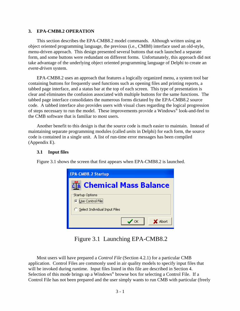
Figure 3.1 shows the screen that first appears when EPA-CMB8.2 is launched.

Most users will have prepared a Control File (Section 4.2.1) for a particular CMBapplication. Control Files are commonly used in air quality models to specify input files thatwill be invoked during runtime. Input files listed in this file are described in Section 4. Selection of this mode brings up a Windows® browse box for selecting a Control File. If aControl File has not been prepared and the user simply wants to run CMB with particular (freely

4See Section 4.2.1 for more details on the structure and function of the Control File.

3 - 2

Figure 3.2 Browse Dialog for Selecting a Control File

associated) input files, the other mode should be selected. Clicking on Cancel returns you to the(previous) Startup dialog.

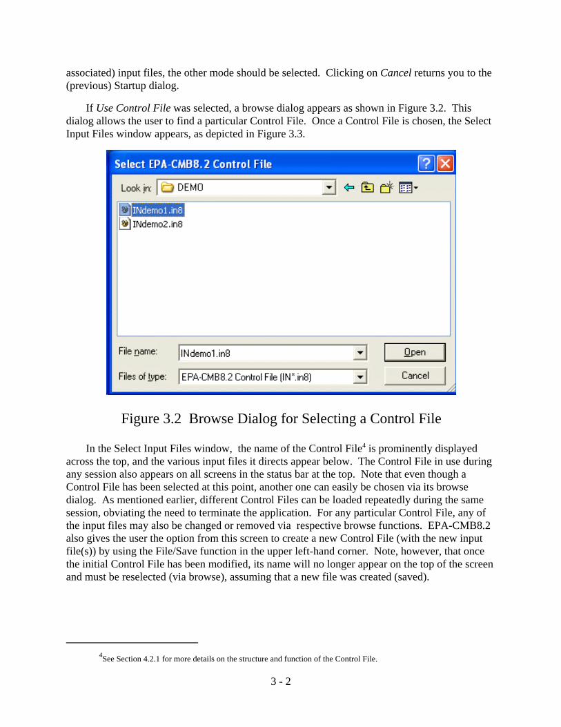
If Use Control File was selected, a browse dialog appears as shown in Figure 3.2. Thisdialog allows the user to find a particular Control File. Once a Control File is chosen, the SelectInput Files window appears, as depicted in Figure 3.3.

In the Select Input Files window, the name of the Control File4 is prominently displayedacross the top, and the various input files it directs appear below. The Control File in use duringany session also appears on all screens in the status bar at the top. Note that even though aControl File has been selected at this point, another one can easily be chosen via its browsedialog. As mentioned earlier, different Control Files can be loaded repeatedly during the samesession, obviating the need to terminate the application. For any particular Control File, any ofthe input files may also be changed or removed via respective browse functions. EPA-CMB8.2also gives the user the option from this screen to create a new Control File (with the new inputfile(s)) by using the File/Save function in the upper left-hand corner. Note, however, that oncethe initial Control File has been modified, its name will no longer appear on the top of the screenand must be reselected (via browse), assuming that a new file was created (saved).

3 - 3

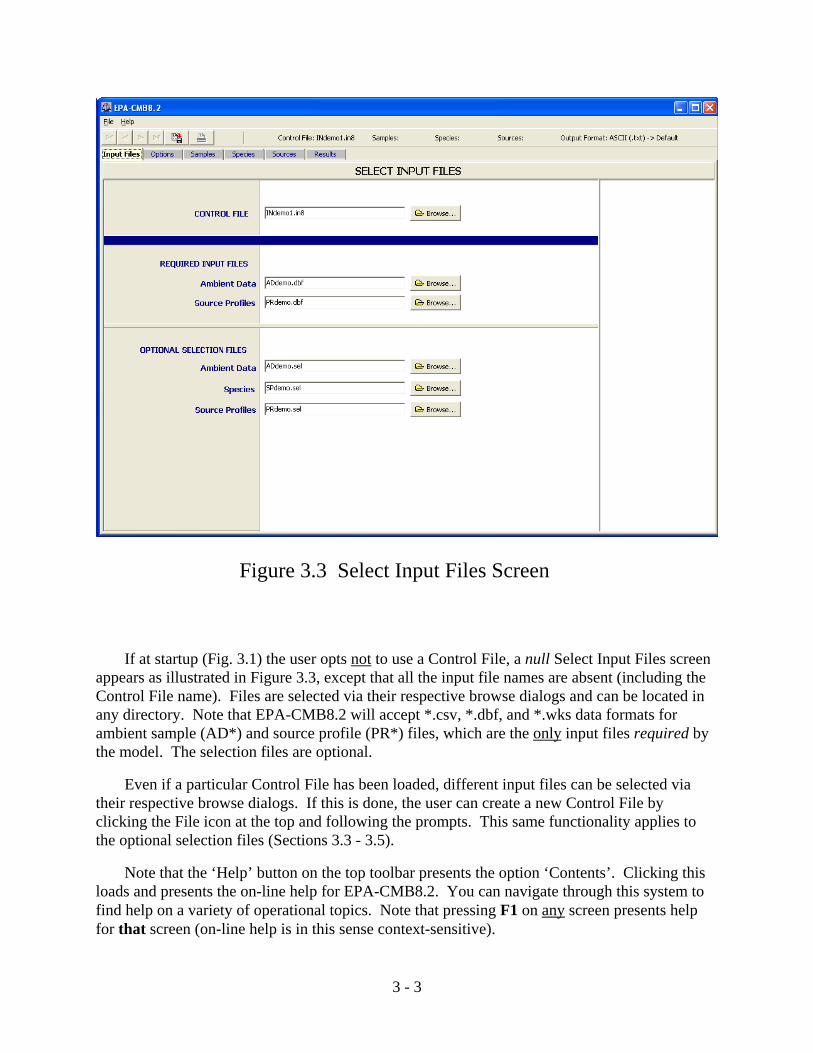
Figure 3.3 Select Input Files Screen

If at startup (Fig. 3.1) the user opts not to use a Control File, a null Select Input Files screenappears as illustrated in Figure 3.3, except that all the input file names are absent (including theControl File name). Files are selected via their respective browse dialogs and can be located inany directory. Note that EPA-CMB8.2 will accept *.csv, *.dbf, and *.wks data formats forambient sample (AD*) and source profile (PR*) files, which are the only input files required bythe model. The selection files are optional.

Even if a particular Control File has been loaded, different input files can be selected viatheir respective browse dialogs. If this is done, the user can create a new Control File byclicking the File icon at the top and following the prompts. This same functionality applies tothe optional selection files (Sections 3.3 - 3.5).

Note that the ‘Help’ button on the top toolbar presents the option ‘Contents’. Clicking thisloads and presents the on-line help for EPA-CMB8.2. You can navigate through this system tofind help on a variety of operational topics. Note that pressing F1 on any screen presents helpfor that screen (on-line help is in this sense context-sensitive).

3 - 4

Figure 3.4 Banner Page for EPA0CMB8.2

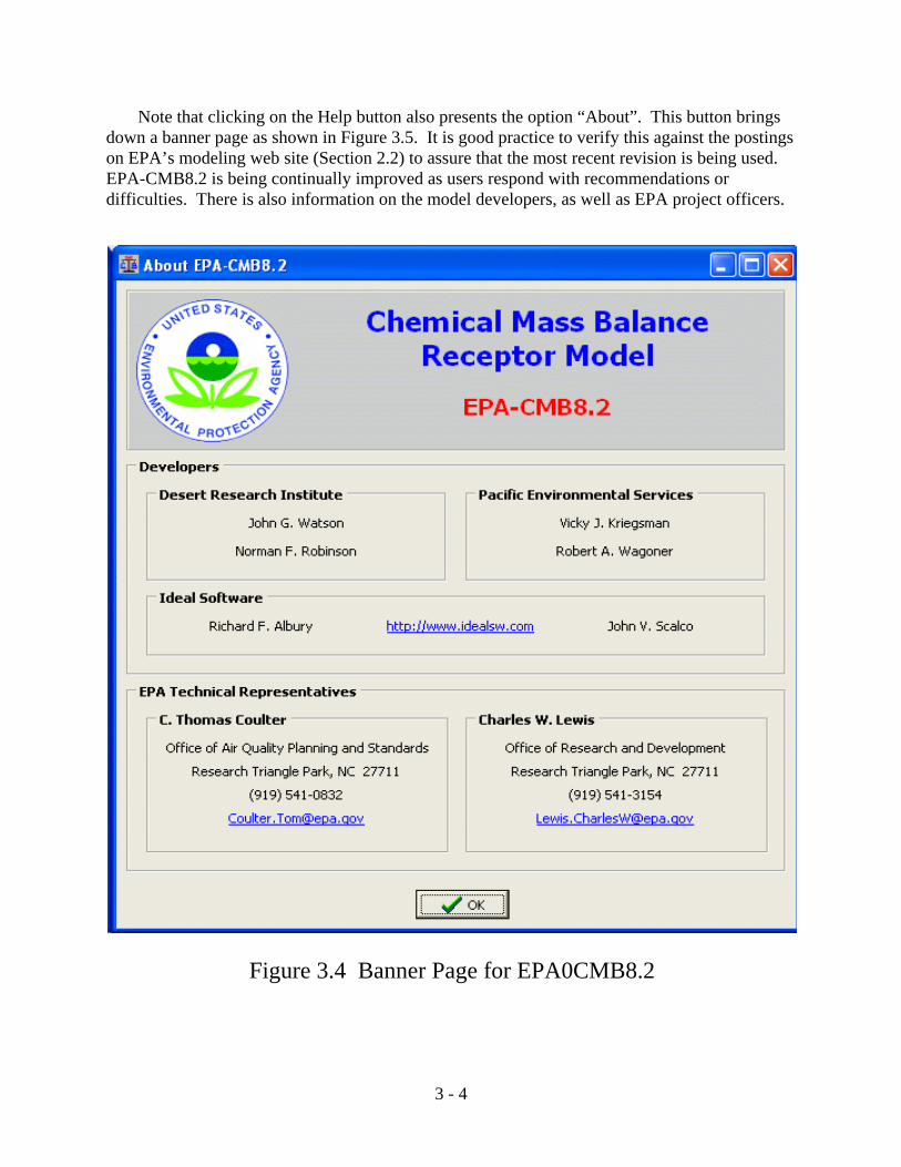
Note that clicking on the Help button also presents the option “About”. This button bringsdown a banner page as shown in Figure 3.5. It is good practice to verify this against the postingson EPA’s modeling web site (Section 2.2) to assure that the most recent revision is being used. EPA-CMB8.2 is being continually improved as users respond with recommendations ordifficulties. There is also information on the model developers, as well as EPA project officers.

3 - 5

Figure 3.5 Options for Current Session

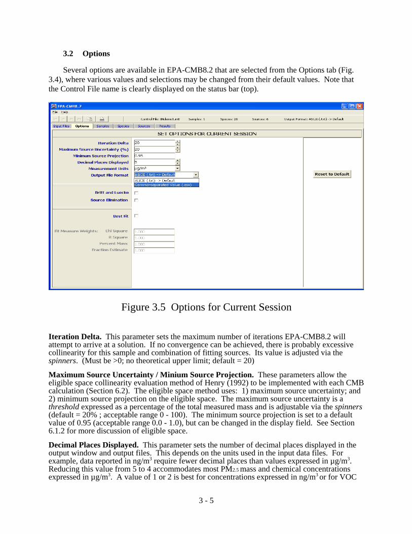
3.2 Options

Several options are available in EPA-CMB8.2 that are selected from the Options tab (Fig.3.4), where various values and selections may be changed from their default values. Note thatthe Control File name is clearly displayed on the status bar (top).

Iteration Delta. This parameter sets the maximum number of iterations EPA-CMB8.2 willattempt to arrive at a solution. If no convergence can be achieved, there is probably excessivecollinearity for this sample and combination of fitting sources. Its value is adjusted via thespinners. (Must be >0; no theoretical upper limit; default = 20)

Maximum Source Uncertainty / Minium Source Projection. These parameters allow theeligible space collinearity evaluation method of Henry (1992) to be implemented with each CMBcalculation (Section 6.2). The eligible space method uses: 1) maximum source uncertainty; and2) minimum source projection on the eligible space. The maximum source uncertainty is athreshold expressed as a percentage of the total measured mass and is adjustable via the spinners(default = 20% ; acceptable range 0 - 100). The minimum source projection is set to a defaultvalue of 0.95 (acceptable range 0.0 - 1.0), but can be changed in the display field. See Section6.1.2 for more discussion of eligible space.

Decimal Places Displayed. This parameter sets the number of decimal places displayed in theoutput window and output files. This depends on the units used in the input data files. Forexample, data reported in ng/m3 require fewer decimal places than values expressed in µg/m3. Reducing this value from 5 to 4 accommodates most PM2.5 mass and chemical concentrationsexpressed in µg/m3. A value of 1 or 2 is best for concentrations expressed in ng/m3 or for VOC

3 - 6

expressed in ppbC or µg/m3. This setting affects the display columns for source contributionsestimates, measured species concentrations (ambient samples and source profiles), calculatedcontributions by species, as well as for inverse singular values. This parameter may be adjustedby using the spinners. The default value is 5 and the maximum value is 6.

Units. The units used for reporting results may be changed via a pull-down menu. Other typicalunits are available, or one may be created (the number of characters is limited to 5 or less).

Output File Format. The file format for spreadsheet-type output is selected in the pull-downbox. As discussed in Section 4.5, the default is ASCII (txt); comma-separated value (CSV) isalso available (which ports nicely to Microsoft Excel®). This selection is echoed on the statusbar at the top of the screen.

Britt and Luecke. Checking this box applies the Britt and Luecke (1973) linear least squaressolution that is explained by Watson et al. (1984) when applied to CMB calculations. Thisoption allows the source profiles used in the fit calculation to vary, and enables a generalsolution to the least squares estimation that includes uncertainty in all the variables (i.e., thesource compositions as well as the ambient concentrations). The default (option disabled) is thesame approximation to the Britt-Luecke algorithm used in CMB7. Note that while the exactBritt-Luecke algorithm must generate a fit whose P2 value is equal to or better (i.e., smaller) thanthat from the approximation algorithm, there is no guarantee that the solution with the better P2

will be superior in terms of its physical meaning. Invocation of this option affects the fitobtained and, as in the case of EPA-CMB8.2's new treatment of collinearity, user experience isnecessary to judge the utility in exercising the new Britt-Luecke algorithm. The Britt-Lueckealgorithm, as implemented in EPA-CMB8.2, has not undergone comprehensive testing, and isnot recommended for inexperienced users. Its inclusion as an option is mainly intended toprovide the opportunity for interested advanced users to perform research investigations neededto establish its future viability. Note also that species concentrations that will appear in the MainReport reflect this algorithm’s modification to the source profile matrix. The individual speciesconcentrations for each source which appear in the (spreadsheet-type) output file are calculatedusing the UNmodified source profile matrix (and therefore will be different). This was done tomaintain continuity with CMB6.

Source Elimination. Checking this box eliminates negative source contributions from thecalculation, one at a time. After each fit attempt, if any sources have negative contributions, thesource with the largest negative contribution is eliminated and another fit is attempted. Thisprocess is repeated until EPA-CMB8.2 finds no sources with negative contributions. Invocationof this option affects the fit obtained by effectively removing collinear sources (Section 6.1.2).

Best Fit. Checking this box causes the program to cycle through the corresponding pairs (samearray index) of fitting species and source profile arrays specified in the source and speciesselection input windows until the best composite Fit Measure has been achieved. When Best Fitis invoked, EPA-CMB8.2 ignores any arrays of species and sources that may have beenselected. The first fitting species array is paired with the first fitting sources array, and so on. EPA-CMB8.2 only attempts a search for a best fit among available corresponding pairs. Anyarrays without a corresponding array to make a pair are ignored. The fit with the largest FitMeasure is then displayed and becomes the current fit. After a Best Fit has been made, thefitting species and fitting sources arrays will be tagged (highlighted) in their respective windows. The Fit Measure algorithm is described in Section 6.3.

Fit Measure Weight. These are the weights (coefficients) applied to each of the performancemeasures chi square, r-square, percent mass, and fraction of eligible sources (number in eligiblespace divided by number of fitting sources). Adjustment of these weights is not enabled in EPA-CMB8.2 unless Best Fit is invoked. Positive values between 0 and 1 may be entered by typinginto the appropriate display fields. Defaults are 1.0 for each performance measure weight. SeeSection 6.1 for more discussion.

3 - 7

Figure 3.6 Ambient Data Selection

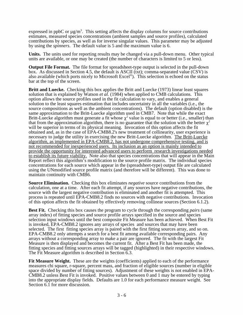
3.3 Select Ambient Data Samples

The screen for selecting a subset of samples on which source apportionment will beperformed is shown in Figure 3.6. If an (optional) AD*.sel file is being directed from the

Control File, one or more samples may appear selected initially (see Section 4.2.4). Otherwise,individual samples are “tagged” by clicking in the respective fields under “SELECTED”. Clicking again deselects the sample. Use of Select /Clear All Samples may also be used to helpestablish the desired list of samples. Note that a counter displays on the status bar (top) thenumber of samples selected at any given time. As indicated, the collection date, duration, starthour, and size fraction (particles) are displayed for each sample. Show/Hide Data togglebetween modes in which speciated data (alternating concentration and uncertainty) for thesamples are either shown or masked. Toggling between View Selected/View All determineswhether data will be displayed for selected (tagged) samples only, or for all samples in the list. Clicking View Graph will provide a bar chart for any sample (selected or not) for which anyfield is filled with blue (note that because of the physical constraints of the graph, somedistortion will occur if the number of species exceeds ~25). This graph is useful to verify thatinput data files have been properly read. Note that use of the “VCR” control buttons on the toptoolbar can help navigate down a long list of samples.

3 - 8

Figure 3.7 Fitting Species Arrays

There will be times when you data will include (dichotomous) measurements for Fine andCoarse size fractions. When this is the case and you want to apportion Fine and Coarse samplesin a batch run, you must take care that compatible sample pairs (matched by site ID, date,sampling duration, and start hour) are selected. These pairs may be Fine/Coarse ... orCoarse/Fine ...

Upon exit, EPA-CMB8.2 will detect changes that may have occurred in arrays initialized bythe optional input files during the session:

1) If an initial array of selected samples (as directed by AD*.sel) has been modified, the user willbe prompted and asked if AD*.sel should be updated (overwritten). The file may also beconveniently renamed.

2) If no selection file was in use but an array of tagged samples has been created during thesession, the user will be prompted and asked whether a samples selection file should be saved. Ifso, an appropriate name (e.g., AD*.sel) should be entered; the extension .sel will be appendedautomatically.

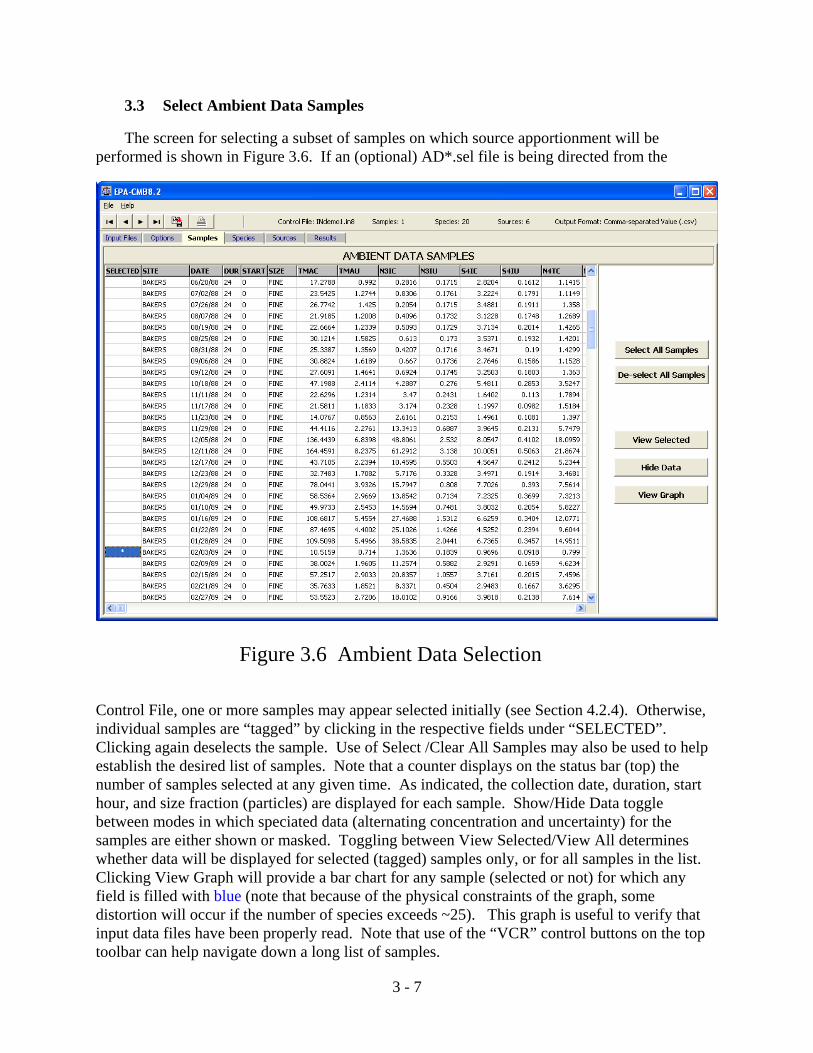
3.4 Select Fitting Species

Fitting species are used in the calculation of source contribution estimates. Species notincluded in this calculation are termed floating species (Section 4.3.2). The comparison ofcalculated and measured values for floating species is part of the model validation process. Fitting species should be selected that are major or unique components of the source typesinfluencing the receptor concentrations. The screen for selecting fitting species is shown inFigure 3.7. This screen is initiated by data read from the (optional) species selection file

3 - 9

(SP*.sel; see Section 4.2.4). Species contained in the selection file are listed down the left-handside and a field of up to 10 arrays is provided. At startup, the first array (in a series) willalways be initially selected as a default. Other arrays may be selected by clicking on the arrayindex (1 - 10). Within a given array that is first activated by clicking its index number, speciesmay be added or removed by clicking in the appropriate field. Select/Clear All Array X mayalso help in configuring a selection array. Note that use of the “VCR” control buttons can helpnavigate down a long list of species, and that a counter displays on the status bar (top) thenumber of species tagged for any selected array. For a selected array, toggling between ViewSelected/View All determines which species will be displayed. This can be handy for a long listof species that would be impossible to display on the screen. If comments are provided in theselection file, they will be displayed on the right-hand side.

Multiple arrays for fitting species are useful when CMB calculations are performed onsamples from several locations or during different times of the year that have differentcontributors. They are also used by the Best Fit option to cycle through different sourcecombinations until the weighted Fit Measure is optimized (Section 3.2).


1) If an initial array of selected species (as directed by SP*.sel) has been modified, the user willbe prompted and asked if SP*.sel should be updated (overwritten). The file may also beconveniently renamed.

2) If no selection file was in use but an array of tagged species has been created during thesession, the user will be prompted and asked whether a samples selection file should be saved. Ifso, an appropriate name (e.g., SP*.sel) should be entered; the extension .sel will be appendedautomatically.

3 - 10

Figure 3.8 Fitting Sources Arrays

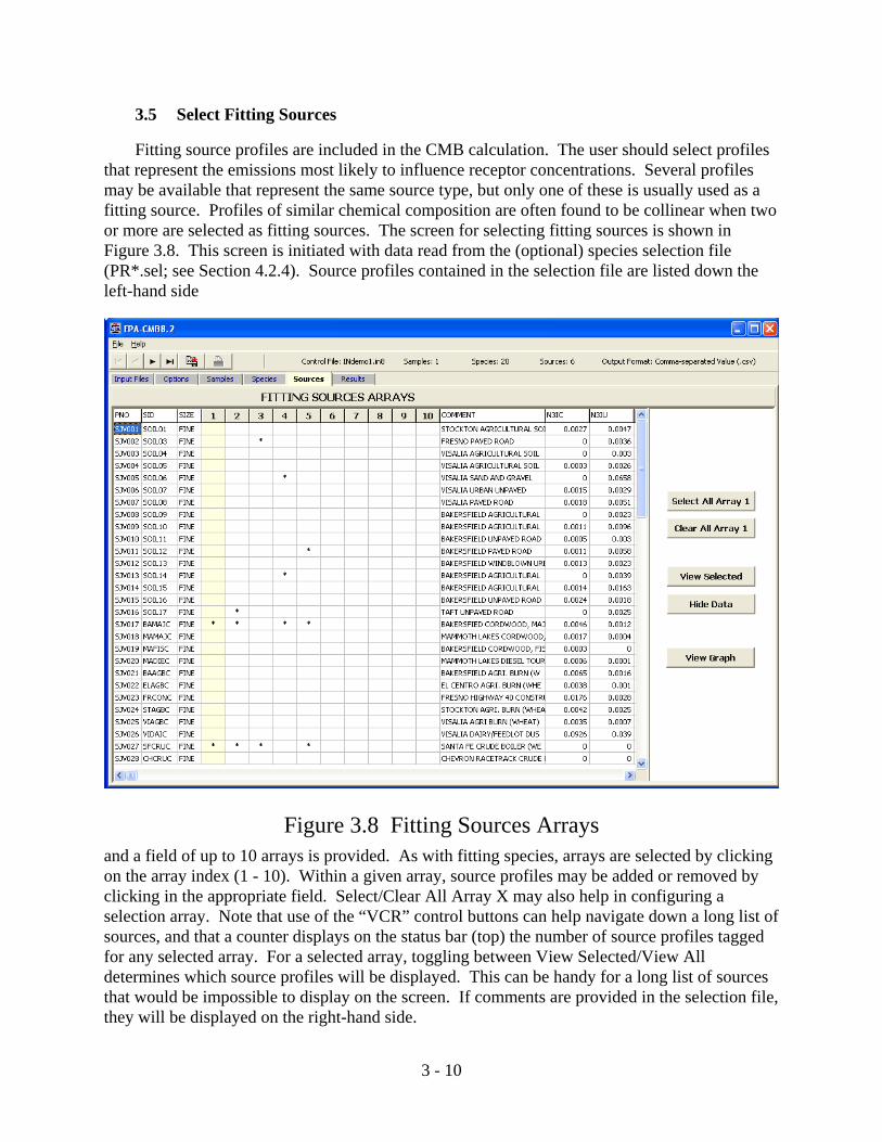
3.5 Select Fitting Sources

Fitting source profiles are included in the CMB calculation. The user should select profilesthat represent the emissions most likely to influence receptor concentrations. Several profilesmay be available that represent the same source type, but only one of these is usually used as afitting source. Profiles of similar chemical composition are often found to be collinear when twoor more are selected as fitting sources. The screen for selecting fitting sources is shown inFigure 3.8. This screen is initiated with data read from the (optional) species selection file(PR*.sel; see Section 4.2.4). Source profiles contained in the selection file are listed down theleft-hand side

and a field of up to 10 arrays is provided. As with fitting species, arrays are selected by clickingon the array index (1 - 10). Within a given array, source profiles may be added or removed byclicking in the appropriate field. Select/Clear All Array X may also help in configuring aselection array. Note that use of the “VCR” control buttons can help navigate down a long list ofsources, and that a counter displays on the status bar (top) the number of source profiles taggedfor any selected array. For a selected array, toggling between View Selected/View Alldetermines which source profiles will be displayed. This can be handy for a long list of sourcesthat would be impossible to display on the screen. If comments are provided in the selection file,they will be displayed on the right-hand side.

3 - 11

Figure 3.9 Calculation Results Tab

As for ambient samples, clicking View Graph will provide a bar chart for any source profile(selected or not) for which any field is filled with blue (note that because of the physicalconstraints of the graph, some distortion will occur if the number of species exceeds ~25). Thisgraph is useful for visual inspection; it helps to verify that input data files have been properlyread and to identify abundant components in each profile. View Grid returns to the array screen.


1) If an initial array of selected source profiles (as directed by PR*.sel) has been modified, theuser will be prompted and asked if PR*.sel should be updated (overwritten). The file may alsobe conveniently renamed.

2) If no selection file was in use but an array of tagged source profiles has been created duringthe session, the user will be prompted and asked whether a samples selection file should besaved. If so, an appropriate name (e.g., PR*.sel) should be entered; the extension .sel will beappended automatically.

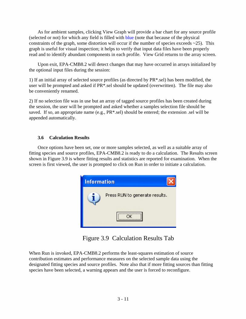
3.6 Calculation Results

Once options have been set, one or more samples selected, as well as a suitable array offitting species and source profiles, EPA-CMB8.2 is ready to do a calculation. The Results screenshown in Figure 3.9 is where fitting results and statistics are reported for examination. When thescreen is first viewed, the user is prompted to click on Run in order to initiate a calculation.

When Run is invoked, EPA-CMB8.2 performs the least-squares estimation of sourcecontribution estimates and performance measures on the selected sample data using thedesignated fitting species and source profiles. Note also that if more fitting sources than fittingspecies have been selected, a warning appears and the user is forced to reconfigure.

5Note that in batch mode, certain warning /error messages that require user intervention are suppressed.

3 - 12

Figure 3.10 Calculation Results - Main Report

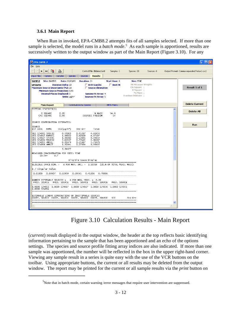
3.6.1 Main Report

When Run in invoked, EPA-CMB8.2 attempts fits of all samples selected. If more than onesample is selected, the model runs in a batch mode.5 As each sample is apportioned, results aresuccessively written to the output window as part of the Main Report (Figure 3.10). For any

(current) result displayed in the output window, the header at the top reflects basic identifyinginformation pertaining to the sample that has been apportioned and an echo of the optionssettings. The species and source profile fitting array indices are also indicated. If more than onesample was apportioned, the number will be reflected in the box in the upper right-hand corner. Viewing any sample result in a series is quite easy with the use of the VCR buttons on thetoolbar. Using appropriate buttons, the current or all results may be deleted from the outputwindow. The report may be printed for the current or all sample results via the print button on

3 - 13

the toolbar; it is also possible to print to Adobe Acrobat® (PDF). A file may be created via thePrint To File option. The header for this file is embellished with an echo of all input files used inthe calculation - another feature of EPA-CMB 8.2.

In analyzing data that may have been collected in sampling networks that employdichotomous samplers, it is common to input speciated data for two complementary sizefractions, fine and coarse (Section 4.2.2). If EPA-CMB8.2 detects that it has such a sample pairfor a given period, it will assume them to be complementary. When a fit is performed, anadditional report is created in which results are summed for the fine and coarse fractions to givethe Total (frequently = PM10). In this case, the fitting array indices are the same as for the fineand coarse component samples, as is the value for Degrees of Freedom. For % Mass explained,the value is determined as follows:

( )( )% .

.

Massmass mass

mass massSF SF calc

SF SF meas

=+

+1 2

1 2

where SF = size fraction

For a given sampling site and period, the samples tagged for analysis must be presented asalternating dichotomous pairs, i.e., Fine/Coarse; Fine/Coarse; Fine/Coarse; ... or Coarse/Fine;Coarse, Fine; Coarse/Fine ... The ‘Total’ report is always appended to that for the 2nd in thedichotomous pair.

In the Main report are several information blocks which present performance measures(Section 6.1.1). First are fitting statistics: r2, P2, percent mass explained, and degrees of freedom. Next is a block that presents the most basic results from EPA-CMB8.2: source contributionestimates. For each source selected is presented a source contribution estimate (SCE) in user-chosen units (Section 3.2), standard errors, and values for T-stat. The series of SCEs aresummed to provide a convenient check on the % mass explained value (EPA-CMB8.2 feature):

%.

MassSCEs

total measured concX=

⎡

⎣⎢⎢

⎤

⎦⎥⎥

∑100

In making this check, be aware that the full uncertainty of the measured concentration value isnot displayed in the Main Report. The field ‘EST’ under ‘SOURCE’ indicates (YES or NO)whether a source’s contribution was estimable in EPA-CMB8.2's attempt at a fit using thesettings in Options. The next block is the Eligible Space Collinearity Display: an echo of themeasured concentration and error for the sample, eligible space dimension for the chosenmaximum uncertainty (Section 3.2), inverse singular values, the number of estimable sources forthe chosen minimum source projection (Section 3.2), and estimable linear combinations of

3 - 14

Figure 3.11 Calculation Results - Contributions by Species

inestimable sources. The concepts of estimable sources and estimable space are discussed inSection 6.1.2. Finally, there is a block detailing species concentrations. Shown for each species(fitting species are tagged with asterisks) is its measured and calculated mass and uncertainty,the ratio of calculated/measured mass (± uncertainty factor), and the ratio of the signed residual(calculated - measured mass) to the uncertainty of that residual. See Section 6.1.3 for moredetails.

Of note is the way EPA-CMB8.2 handles missing values in source and receptor files(designated by –99. in place of the value). When a fitting species value is missing from either anambient sample or source profile, that species is automatically removed from the calculation andthe species selection flag (ordinarily an asterisk) is set to “M” in the report output file. SeeSection 4.2.2 & 4.2.3; Appendix F.

For any of the information blocks in the main report, the presence of a series of asterisks fora numerical value field represents an overflow condition. Reducing the number of decimalplaces displayed (Section 3.2) should correct the problem.

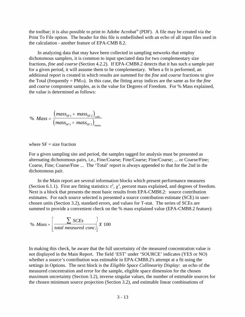
3.6.2 Contributions by Species

Beyond the traditional apportionment results generated by EPA-CMB8.2, it is also ofinterest to analyze the way in which pollutant mass is distributed among sources by species. This distribution is presented in the report Contributions by Species (Figure 3.11). This report

3 - 15

Figure 3.12 Calculation Results - MPIN Matrix

provides one more dimension to the Species Concentrations block in the Main Report. Theseresults are useful when source contributions to species other than total mass are of interest. Thereport also indicates which sources are the major and minor contributors to each species. Sincevalues in this report are ratios of calculated species concentrations to the measured total speciesconcentration, multiplying the values by their respective measured value and summing willconfirm the values listed in the sum of calculated species contributions column (left-hand side).For convenience, both the calculated and measured columns are from the Main Report arereproduced here - another feature of EPA-CMB8.2. As with the Main Report, a print-out ofContributions by Species may be obtained for the current sample result via the print button onthe toolbar, and a file may be created via the Print To File option. For more information seeSection 6.2.

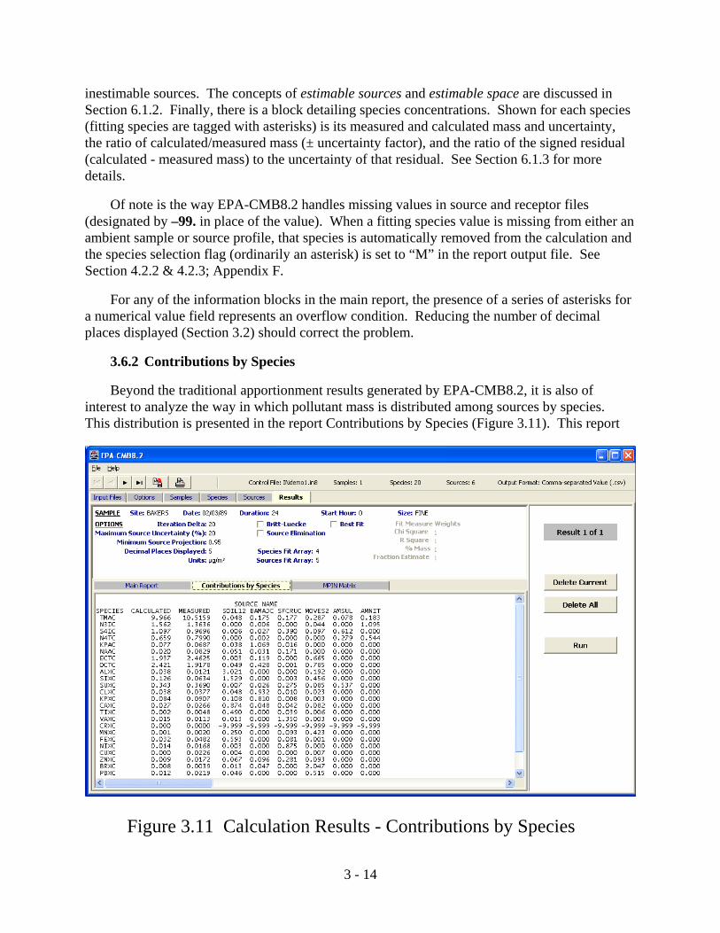
3.6.3 Modified Pseudo-Inverse Normalized (MPIN) Matrix

Another report that may be of interest is the Modified Pseudo-Inverse Normalized (MPIN)matrix (Figure 3.12). The MPIN matrix identifies which fitting species have the largestinfluence on the source contribution estimates from each profile (Section 6.2). Examining theseweights suggests sensitivity tests to determine the extent to which source contributions vary withchanges in profile abundances or the selection of fitting species. As with the Main Report andContributions by Species, a print-out of the MPIN matrix may be obtained for the current sampleresult via the print button on the toolbar, and a file may be created via the Print To File option.

4 - 1

4. INPUT AND OUTPUT FILES

This section describes the structure of EPA-CMB8.2 input and output files and methods ofgenerating these files. Each type of input file structure is illustrated with one of the test data setspackaged with EPA-CMB8.2.

4.1 File Naming Conventions

EPA-CMB8.2 input and output files can have any file name with a three-character extensionthat indicates the file type. A suggested naming convention is PP*.ext, where:

! PP: Type of file. Common definitions are:

IN Control file identifying specific input data files.

AD Ambient Data. Selection file initiates sample selection from the ambient data filefor apportionment during an CMB session; data file contains the measuredambient concentrations and their uncertainty values.

PR Source PRofile. Selection file identifies initial fitting profiles and source profiledescriptions; data file contains mass-fraction chemical abundances and theiruncertainties.

SP SPecies selection file identifies initial fitting species for the CMB session.

! * Study identifier. This code allows separate studies to be distinguished from oneanother. EPA-CMB8.2 allows Windows® flexibility for this name string (i.e., it isnot character-limited).

! ext Extension that also identifies file type or format. The following file extensionsare recognized by EPA-CMB8.2:

in8 Input control (ASCII text) file. EPA-CMB8.2 lists files with this extension in theControl File browse window at startup.

sel Fitting profiles, fitting species, and sample selection (ASCII text) files. EPA-CMB8.2 recognizes files with this extension as containing initial selections thatcan be entered external to the program. This extension applies only to the PR, SP,and AD file types.

csv Ambient data or source profile comma-separated value ASCII text file. Eachfield is separated by a comma. Comma-delimited ASCII data base output files arewritten with this extension.

dbf Data base file generated by dBase or FoxPro compatible data managementsoftware. Most commonly used spreadsheets offer this as an output option. dBase or FoxPro output files are written with this extension.

4 - 2

txt Ambient data or source profile data blank-delimited ASCII text file. Formatted,blank-delimited ASCII data base output files may be created with theseextensions.

wks Lotus 1-2-3 version 1 spreadsheet format. Most commonly used spreadsheetsoffer this as an output option. This is the most useful output format for the database output file when source contribution estimates will be analyzed using aspreadsheet.

Note that if neither input file (ambient data or source profile data) is supplied in ASCIIformat (*.txt), EPA-CMB8.2 converts any of the csv, dbf, and wks input data files to the blank-delimited (txt) files which are actually used by the program. These txt files are created “on thefly” as soon as the user moves off of the Input Files Screen (Figure 3.3), and will appear in thesame subdirectory that stores any of the csv, dbf, and/or wks files. Such txt files created fromdbf files are nicely formatted and easy to read. If any txt files are supplied in the subdirectorybut not directed for use as input files in the Control File, they will be overwritten (replaced) bynew versions created by EPA-CMB8.2. If, however, any txt files are supplied and directed foruse as input data by the Control File, they will be retained (not modified).

4.2 Input File Relationship

Six data files are normally used for input to EPA-CMB8.2, the first of which is a control filethat directs EPA-CMB8.2 to five specific files. Three of the files are optional selection files,which provide substantial user convenience by establishing commonly used arrays and samplesubsets that would otherwise need to be initialized each time the model is run. The remainingtwo - the ambient and source profile data files - are required by EPA-CMB8.2. Figure 4.1presents the relationship of the files whose descriptions appear in the following subsections.

4.2.1 Control File: IN*.in8

This fixed format file contains a list of the names of EPA-CMB8.2 input data files, allof which must reside in the same directory that stores the Control File itself. This filename (e.g.,INsjvf.in8, exemplified in Figure 4.1) consists of five lines as shown below. These lines, insuccession, contain the names of the files which are described in the following subsections. If aselection file is absent, the corresponding line in the Control File should be labeled with one ormore characters, e.g., a series of asterisks (‘******’) - or any name that doesn’t reside in theControl File directory. Here’s an example:

PRsjvf.sel

SPsjvf.sel

*******

ADsjvf.csv

PRsjvf.csv

File name entries should be left justified and in the sequence shown. In EPA-CMB8.2, the only restriction on file names is that they are acceptable to the operating system. This means that extended file names may be used. The utility of the Control File is to save theeffort of keying in the input filenames individually. If a Control File is not used at startup, EPA-CMB8.2 will accept the names of individual data input files on the fly, provided they arecompatible with each other.

4 -3

Figure 4.1. EPA-CMB8.2 Input FilesSJV001 SOIL01 * STOCKTON AGRICULTURAL SOIL(PEAT)SJV002 SOIL03 * FRESNO PAVED ROADSJV003 SOIL04 VISALIA AGRICULTURAL SOIL (COTTON/WALNUT)SJV004 SOIL05 VISALIA AGRICULTURAL SOIL (RAISIN)SJV005 SOIL06 * VISALIA SAND AND GRAVEL...

Fitting sources profile selection file (PRsjvf.sel)

TMAC TOT Mass by gravimetry(ug/m3)N3IC NO3 * * * * Nitrate by IC (ug/m3)S4IC SO4 * * * * Sulfate by IC (ug/m3)N4TC NH4 * * * Ammonium by AC (ug/m3)KPAC K-S * * * * Soluble Potassium by AA (ug/m3)...

Fitting species selection file (SPsjvf.sel)

Ambient data selection file (ADsjvf.sel)BAKERS 07/26/88 24 0 FINE *CROWS 07/26/88 24 0 FINE * FELLOW 07/26/88 24 0 FINE * FRESNO 07/26/88 24 0 FINE * KERN 07/26/88 24 0 FINE * STOCKT 07/26/88 24 0 FINE *

ID DATE DUR STHOUR SIZE TMAC TMAU N3IC N3IU S4IC S4IU N4TC N4TU KPAC ...BAKERS 06/20/88 24 0 FINE 17.2788 0.9920 0.2816 0.1715 2.8204 0.1612 ...BAKERS 07/02/88 24 0 FINE 23.5425 1.2744 0.8306 0.1761 3.2224 0.1791 ...BAKERS 07/26/88 24 0 FINE 26.7742 1.4250 0.2054 0.1715 3.4881 0.1911 ...BAKERS 08/07/88 24 0 FINE 21.9185 1.2008 0.4096 0.1732 3.1228 0.1748 ...BAKERS 08/19/88 24 0 FINE 22.6664 1.2339 0.5093 0.1729 3.7134 0.2014 ......

Ambient data input file (ADsjvf.txt)

PNO SID SIZE N3IC N3IU S4IC S4IU N4TC N4TU KPAC KPAU NAAC NAAU ECTC ECTU ...SJV001 SOIL01 FINE 0.002700 0.004700 0.000400 0.001300 0.000600 0.000500 ...SJV002 SOIL03 FINE 0.000000 0.003600 0.005000 0.006600 0.000300 0.000500 ...SJV003 SOIL04 FINE 0.000000 0.003000 0.000000 0.001100 0.000000 0.000100 ...SJV004 SOIL05 FINE 0.000300 0.002600 0.000000 0.000900 0.000000 0.000000...SJV005 SOIL06 FINE 0.000000 0.065800 0.000000 0.023800 0.000000 0.001100 ......

Source profile input file (PRsjvf.txt)

PRsjvf.selSPsjvf.selADsjvf.selADsjvf.txtPRsjvf.txt

Control File

(INsjvf.in8)

4 -3

Figure 4.1. EPA-CMB8.2 Input FilesSJV001 SOIL01 * STOCKTON AGRICULTURAL SOIL(PEAT)SJV002 SOIL03 * FRESNO PAVED ROADSJV003 SOIL04 VISALIA AGRICULTURAL SOIL (COTTON/WALNUT)SJV004 SOIL05 VISALIA AGRICULTURAL SOIL (RAISIN)SJV005 SOIL06 * VISALIA SAND AND GRAVEL...

Fitting sources profile selection file (PRsjvf.sel)SJV001 SOIL01 * STOCKTON AGRICULTURAL SOIL(PEAT)SJV002 SOIL03 * FRESNO PAVED ROADSJV003 SOIL04 VISALIA AGRICULTURAL SOIL (COTTON/WALNUT)SJV004 SOIL05 VISALIA AGRICULTURAL SOIL (RAISIN)SJV005 SOIL06 * VISALIA SAND AND GRAVEL...

Fitting sources profile selection file (PRsjvf.sel) Fitting sources profile selection file (PRsjvf.sel)

TMAC TOT Mass by gravimetry(ug/m3)N3IC NO3 * * * * Nitrate by IC (ug/m3)S4IC SO4 * * * * Sulfate by IC (ug/m3)N4TC NH4 * * * Ammonium by AC (ug/m3)KPAC K-S * * * * Soluble Potassium by AA (ug/m3)...

Fitting species selection file (SPsjvf.sel) Fitting species selection file (SPsjvf.sel)



BAKERS 07/26/88 24 0 FINE *CROWS 07/26/88 24 0 FINE * FELLOW 07/26/88 24 0 FINE * FRESNO 07/26/88 24 0 FINE * KERN 07/26/88 24 0 FINE * STOCKT 07/26/88 24 0 FINE *

ID DATE DUR STHOUR SIZE TMAC TMAU N3IC N3IU S4IC S4IU N4TC N4TU KPAC ...BAKERS 06/20/88 24 0 FINE 17.2788 0.9920 0.2816 0.1715 2.8204 0.1612 ...BAKERS 07/02/88 24 0 FINE 23.5425 1.2744 0.8306 0.1761 3.2224 0.1791 ...BAKERS 07/26/88 24 0 FINE 26.7742 1.4250 0.2054 0.1715 3.4881 0.1911 ...BAKERS 08/07/88 24 0 FINE 21.9185 1.2008 0.4096 0.1732 3.1228 0.1748 ...BAKERS 08/19/88 24 0 FINE 22.6664 1.2339 0.5093 0.1729 3.7134 0.2014 ......

Ambient data input file (ADsjvf.txt) Ambient data input file (ADsjvf.txt)

PNO SID SIZE N3IC N3IU S4IC S4IU N4TC N4TU KPAC KPAU NAAC NAAU ECTC ECTU ...SJV001 SOIL01 FINE 0.002700 0.004700 0.000400 0.001300 0.000600 0.000500 ...SJV002 SOIL03 FINE 0.000000 0.003600 0.005000 0.006600 0.000300 0.000500 ...SJV003 SOIL04 FINE 0.000000 0.003000 0.000000 0.001100 0.000000 0.000100 ...SJV004 SOIL05 FINE 0.000300 0.002600 0.000000 0.000900 0.000000 0.000000...SJV005 SOIL06 FINE 0.000000 0.065800 0.000000 0.023800 0.000000 0.001100 ......

Source profile input file (PRsjvf.txt) Source profile input file (PRsjvf.txt)

PRsjvf.selSPsjvf.selADsjvf.selADsjvf.txtPRsjvf.txt

Control File

(INsjvf.in8)

4 - 4

4.2.2 Ambient Data Input File (AD*.csv, AD*.dbf, AD*.txt, AD*.wks)

Ambient data files may be formatted as comma-separated values in ASCII text (*.csv),xBASE (*.dbf), blank-delimited ASCII text (*.txt), or Lotus Worksheet (*.wks). The csv anddbf formats are preferred, as they are easier to prepare in spreadsheet (e.g., Microsoft Excel®,Corel QuatroPro®, Lotus 123) and data base (e.g., Microsoft Access®, dBASE) software than theother formats. The wks format creates large files and requires substantial translation time forEPA-CMB8.2 input and output, so it is the least desirable of these alternatives. The TXT formatis most consistent with CMB7, so older CMB7 data files can be used for EPA-CMB8.2 inputwithout modification. NB: if using TXT format, make sure the file’s not tab-delimited! Recallfrom Section 4.1 that under some circumstances, EPA-CMB8.2 will create an ambient data inputfile in txt (ASCII) format “on the fly”, and that it is actually this format that the model uses forcalculations. The appropriate file extension must be associated with each format, as EPA-CMB8.2 recognizes the file type by this extension.

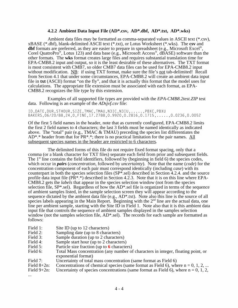
Examples of all supported file types are provided with the EPA-CMB8.2test.ZIP testdata. Following is an example of the ADsjvf.csv file:

ID,DATE,DUR,STHOUR,SIZE,TMAC,TMAU,N3IC,N3IU,.....,PBXC,PBXUBAKERS,06/20/88,24,0,FINE,17.2788,0.9920,0.2816,0.1715,.....,0.0236,0.0052

Of the first 5 field names in the header, note that as currently configured, EPA-CMB8.2 limitsthe first 2 field names to 4 characters; the last 3 fields must be named identically as indicatedabove. The “total” pair (e.g., TMAC & TMAU) preceding the species list differentiates theAD*.* header from that for PR*.*; there is no practical limitation for the pair names. Allsubsequent species names in the header are restricted to 6 characters.

The delimited forms of this file do not require fixed format spacing, only that acomma (or a blank character for TXT files) separate each field from prior and subsequent fields. The 1st line contains the field identifiers, followed by (beginning in field 6) the species codes,which occur in pairs (concentration, followed by uncertainty). Note that the name (code) for theconcentration component of each pair must correspond identically (including case) with itscounterpart in both the species selection files (SP*.sel) described in Section 4.2.4. and the sourceprofile data input file (PR*.*) described in Section 4.2.3. Note that it is on this line where EPA-CMB8.2 gets the labels that appear in the species selection window (not from the speciesselection file, SP*.sel). Regardless of how the AD*.sel file is organized in terms of the sequenceof ambient samples listed, in the sample selection screen they will appear according to thesequence dictated by the ambient data file (e.g., AD*.txt). Note also this line is the source of allspecies labels appearing in the Main Report. Beginning with the 2nd line are the actual data, oneline per ambient sample, starting with the Site ID in Field 1. Note also that it is this ambient datainput file that controls the sequence of ambient samples displayed in the samples selectionwindow (not the samples selection file, AD*.sel). The records for each sample are formatted asfollows:

Field 1: Site ID (up to 12 characters)Field 2: Sampling date (up to 8 characters)Field 3: Sample duration (up to 2 characters)Field 4: Sample start hour (up to 2 characters)Field 5: Particle size fraction (up to 6 characters) Field 6: Total Mass concentration (any number of characters in integer, floating point, or

exponential format)Field 7: Uncertainty of total mass concentration (same format as Field 6)Field 8+2n: Concentrations of chemical species (same format as Field 6), where n = 0, 1, 2, ...Field 9+2n: Uncertainty of species concentrations (same format as Field 6), where n = 0, 1, 2,...

6If more that 4 size ranges are supplied for a given sampling site and period, the following error message from the DLLwill appear (Appendix E):Number of fitting sources = 0 > Number of fitting species = 0, followed by:The number of fitting sources must be positive and <= number of fitting species.

4 - 5

EPA-CMB8.2 always assumes that Field 6 is the total mass concentration, and it doesnot use this as a fitting species. Uncertainty values in fields 7 and 9+2n are in the same units asthe measured concentration values. For EPA-CMB8.2, the total number of ambient data recordscan reach into the thousands, limited only by computer memory. This makes it especially usefulfor examining multi-species hourly data obtained from automated gas chromatographs and time-of-flight mass spectrometers. For particles, up to four different size fraction identifiers may beused for the same sampling site and period, and the user can select mnemonics that suitindividual purposes.6 The size fraction names FINE and COARSE are reserved for the PM2.5 andcoarse particle (PM10 to PM2.5) size fractions that are commonly measured in PM10 sourceassessment studies. As mentioned in Section 3.6.1, when these size fraction identifiers (i.e.,‘FINE’ & ‘COARSE’) are used, an additional report is produced that sums the fine and coarsesource contribution estimate(s) (and uncertainties) to provide the estimate(s) for ‘Total’(frequently = PM10). Any other designator can be placed in the size column for non-segregatedsamples, such as “PM25” or “VOC”. Where semi-volatile materials are being apportioned, theparticle (PART) and gas (GAS) phases are good designations.

Positive uncertainty values (> 0) must be assigned to all (non-missing) chemicalconcentrations used as fitting species. EPA-CMB8.2 will return an error message when itdetects (in the input data file for ambient samples) a value for uncertainty that is less than orequal to zero for any species concentration value not flagged as missing. A species for which theconcentration value is missing (i.e., invalid) cannot be used as a fitting species for that sample. Missing values for either concentrations or associated uncertainty must be designated by placing -99. in the appropriate field in the data file. If a species is to be flagged as “missing”, the value -99. must appear in the concentration field; substituting -99. for its uncertainty is optionalbecause, as mentioned in Section 3.6.1, the species will automatically be removed from thecalculation (though they will appear in the Main Report). For any species, when the fields formissing values species are substituted in this way, -99.0000 will appear in applicable fieldsunder “MEASURED” in the Main Report so long as decimal places displayed (Section 3.2) is setto a value < 5. When the species concentration is flagged with -99., the value forCALCULATED/MEASURED in the Main Report will always be 0.00. The value for thisdiagnostic as well as for RESIDUAL/UNCERTAINTY will in this case be meaningless. SeeAppendix F for a discussion of EPA-CMB8.2's interpretation and treatment of input dataconditions.

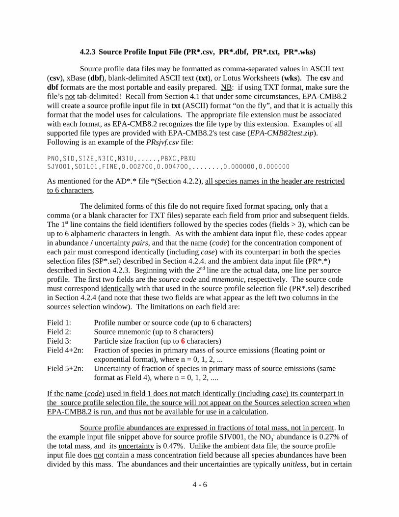
4 - 6

4.2.3 Source Profile Input File (PR*.csv, PR*.dbf, PR*.txt, PR*.wks)

Source profile data files may be formatted as comma-separated values in ASCII text(csv), xBase (dbf), blank-delimited ASCII text (txt), or Lotus Worksheets (wks). The csv anddbf formats are the most portable and easily prepared. NB: if using TXT format, make sure thefile’s not tab-delimited! Recall from Section 4.1 that under some circumstances, EPA-CMB8.2will create a source profile input file in txt (ASCII) format “on the fly”, and that it is actually thisformat that the model uses for calculations. The appropriate file extension must be associatedwith each format, as EPA-CMB8.2 recognizes the file type by this extension. Examples of allsupported file types are provided with EPA-CMB8.2's test case (EPA-CMB82test.zip). Following is an example of the PRsjvf.csv file:

PNO,SID,SIZE,N3IC,N3IU,.....,PBXC,PBXUSJV001,SOIL01,FINE,0.002700,0.004700,.......,0.000000,0.000000

As mentioned for the AD*.* file *(Section 4.2.2), all species names in the header are restrictedto 6 characters.

The delimited forms of this file do not require fixed format spacing, only that acomma (or a blank character for TXT files) separate each field from prior and subsequent fields. The 1st line contains the field identifiers followed by the species codes (fields > 3), which can beup to 6 alphameric characters in length. As with the ambient data input file, these codes appearin abundance / uncertainty pairs, and that the name (code) for the concentration component ofeach pair must correspond identically (including case) with its counterpart in both the speciesselection files (SP*.sel) described in Section 4.2.4. and the ambient data input file (PR*.*)described in Section 4.2.3. Beginning with the 2nd line are the actual data, one line per sourceprofile. The first two fields are the source code and mnemonic, respectively. The source codemust correspond identically with that used in the source profile selection file (PR*.sel) describedin Section 4.2.4 (and note that these two fields are what appear as the left two columns in thesources selection window). The limitations on each field are:

Field 1: Profile number or source code (up to 6 characters)Field 2: Source mnemonic (up to 8 characters)Field 3: Particle size fraction (up to 6 characters)Field 4+2n: Fraction of species in primary mass of source emissions (floating point or

exponential format), where n = 0, 1, 2, ...Field 5+2n: Uncertainty of fraction of species in primary mass of source emissions (same

format as Field 4), where n = 0, 1, 2, ....

If the name (code) used in field 1 does not match identically (including case) its counterpart inthe source profile selection file, the source will not appear on the Sources selection screen whenEPA-CMB8.2 is run, and thus not be available for use in a calculation.

Source profile abundances are expressed in fractions of total mass, not in percent. Inthe example input file snippet above for source profile SJV001, the NO3

- abundance is 0.27% ofthe total mass, and its uncertainty is 0.47%. Unlike the ambient data file, the source profileinput file does not contain a mass concentration field because all species abundances have beendivided by this mass. The abundances and their uncertainties are typically unitless, but in certain

4 - 7

applications can be represented as concentrations. The user will have to account for this lattercase in interpreting the SCEs that are computed. The total number of records included dependson the number of species, number of sources, and size of the computer memory.

From one to four different size fraction identifiers may be used, but these must be thesame as those used in the ambient data and sample selection files. Missing values for chemicalspecies in source profile files can be replaced by a best estimate with a large uncertainty if theyare to be used as fitting species. Missing values must be flagged with –99. if the species is not intended for use as fitting species. Species with mass fractions so flagged will automatically beremoved from the calculation (though they will appear in the Main Report). While uncertaintyvalues for species in source profiles are allowed to be # 0.0, some effort should be made tosupply values > 0.0. Default values of 0.0 for the fraction and 0.0001 to 0.01 for the uncertaintyare often chosen for species that are expected to be present in small abundances. This indicatesthat the species is present in source emissions at a concentration less than 0.01% to 1%. Asmaller value may be appropriate for certain source types and species. See Appendix F for adiscussion of EPA-CMB8.2's interpretation and treatment of input data conditions.

In certain cases in which an uncertainty value >0 is applied to a species whose abundance =0, the uncertainty represents the lower quantifiable limit of the measurement. A zero value forabundance means that the true value is something between zero and the detection limit. Zerosare important in some source profiles when they occur in other source profiles. This makes thatspecies a marker for the source in which it occurs. The uncertainty for the zero adds to theeffective variance weighting. If this uncertainty is high and the source contribution estimate ishigh, the influence of that species is reduced by the weighting.

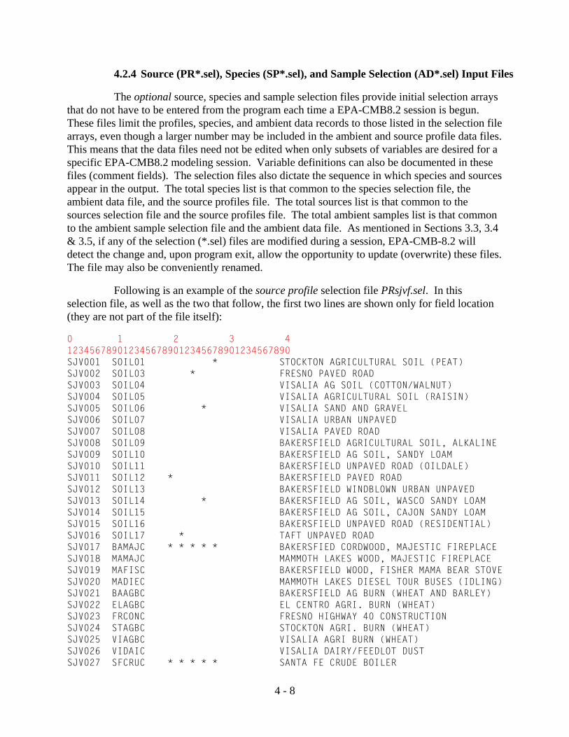
4 - 8

4.2.4 Source (PR*.sel), Species (SP*.sel), and Sample Selection (AD*.sel) Input Files

The optional source, species and sample selection files provide initial selection arraysthat do not have to be entered from the program each time a EPA-CMB8.2 session is begun. These files limit the profiles, species, and ambient data records to those listed in the selection filearrays, even though a larger number may be included in the ambient and source profile data files. This means that the data files need not be edited when only subsets of variables are desired for aspecific EPA-CMB8.2 modeling session. Variable definitions can also be documented in thesefiles (comment fields). The selection files also dictate the sequence in which species and sourcesappear in the output. The total species list is that common to the species selection file, theambient data file, and the source profiles file. The total sources list is that common to thesources selection file and the source profiles file. The total ambient samples list is that commonto the ambient sample selection file and the ambient data file. As mentioned in Sections 3.3, 3.4& 3.5, if any of the selection (*.sel) files are modified during a session, EPA-CMB-8.2 willdetect the change and, upon program exit, allow the opportunity to update (overwrite) these files. The file may also be conveniently renamed.

Following is an example of the source profile selection file PRsjvf.sel. In thisselection file, as well as the two that follow, the first two lines are shown only for field location(they are not part of the file itself):

0 1 2 3 41234567890123456789012345678901234567890SJV001 SOIL01 * STOCKTON AGRICULTURAL SOIL (PEAT)SJV002 SOIL03 * FRESNO PAVED ROADSJV003 SOIL04 VISALIA AG SOIL (COTTON/WALNUT)SJV004 SOIL05 VISALIA AGRICULTURAL SOIL (RAISIN)SJV005 SOIL06 * VISALIA SAND AND GRAVELSJV006 SOIL07 VISALIA URBAN UNPAVEDSJV007 SOIL08 VISALIA PAVED ROADSJV008 SOIL09 BAKERSFIELD AGRICULTURAL SOIL, ALKALINESJV009 SOIL10 BAKERSFIELD AG SOIL, SANDY LOAMSJV010 SOIL11 BAKERSFIELD UNPAVED ROAD (OILDALE)SJV011 SOIL12 * BAKERSFIELD PAVED ROADSJV012 SOIL13 BAKERSFIELD WINDBLOWN URBAN UNPAVEDSJV013 SOIL14 * BAKERSFIELD AG SOIL, WASCO SANDY LOAMSJV014 SOIL15 BAKERSFIELD AG SOIL, CAJON SANDY LOAMSJV015 SOIL16 BAKERSFIELD UNPAVED ROAD (RESIDENTIAL)SJV016 SOIL17 * TAFT UNPAVED ROADSJV017 BAMAJC * * * * * BAKERSFIED CORDWOOD, MAJESTIC FIREPLACESJV018 MAMAJC MAMMOTH LAKES WOOD, MAJESTIC FIREPLACESJV019 MAFISC BAKERSFIELD WOOD, FISHER MAMA BEAR STOVESJV020 MADIEC MAMMOTH LAKES DIESEL TOUR BUSES (IDLING)SJV021 BAAGBC BAKERSFIELD AG BURN (WHEAT AND BARLEY)SJV022 ELAGBC EL CENTRO AGRI. BURN (WHEAT)SJV023 FRCONC FRESNO HIGHWAY 40 CONSTRUCTIONSJV024 STAGBC STOCKTON AGRI. BURN (WHEAT)SJV025 VIAGBC VISALIA AGRI BURN (WHEAT)SJV026 VIDAIC VISALIA DAIRY/FEEDLOT DUSTSJV027 SFCRUC * * * * * SANTA FE CRUDE BOILER

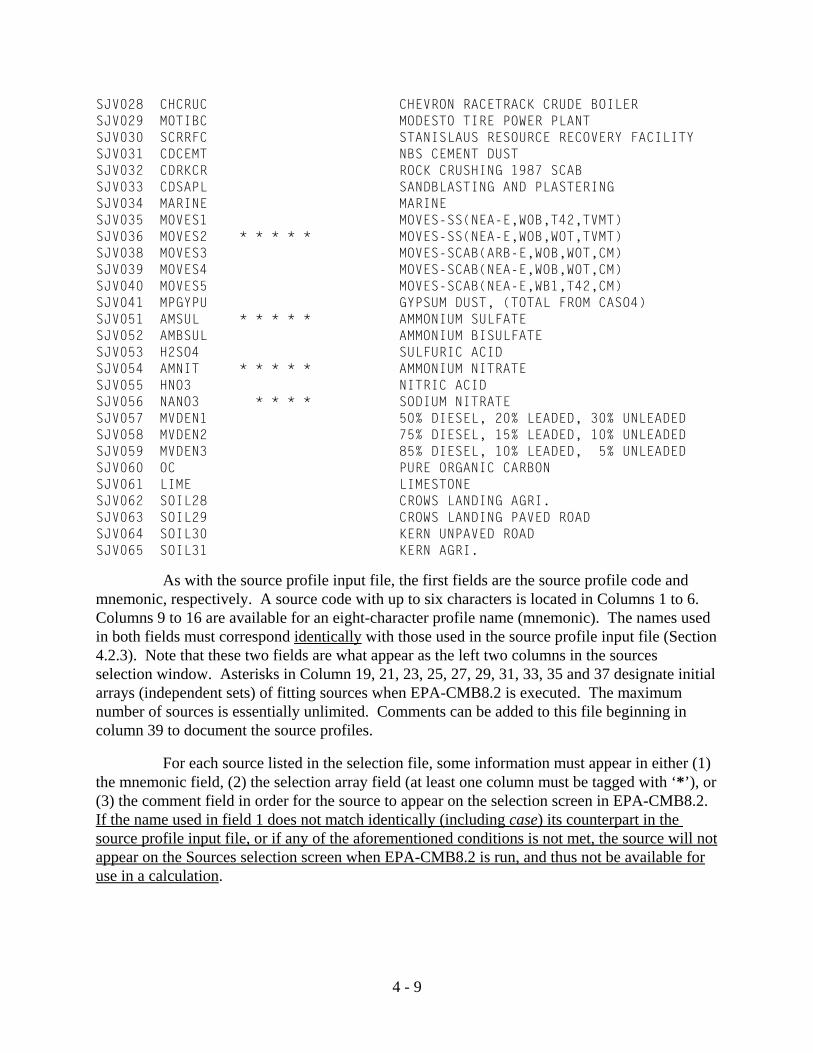
4 - 9

SJV028 CHCRUC CHEVRON RACETRACK CRUDE BOILERSJV029 MOTIBC MODESTO TIRE POWER PLANTSJV030 SCRRFC STANISLAUS RESOURCE RECOVERY FACILITYSJV031 CDCEMT NBS CEMENT DUSTSJV032 CDRKCR ROCK CRUSHING 1987 SCABSJV033 CDSAPL SANDBLASTING AND PLASTERINGSJV034 MARINE MARINESJV035 MOVES1 MOVES-SS(NEA-E,WOB,T42,TVMT)SJV036 MOVES2 * * * * * MOVES-SS(NEA-E,WOB,WOT,TVMT)SJV038 MOVES3 MOVES-SCAB(ARB-E,WOB,WOT,CM)SJV039 MOVES4 MOVES-SCAB(NEA-E,WOB,WOT,CM)SJV040 MOVES5 MOVES-SCAB(NEA-E,WB1,T42,CM)SJV041 MPGYPU GYPSUM DUST, (TOTAL FROM CASO4)SJV051 AMSUL * * * * * AMMONIUM SULFATESJV052 AMBSUL AMMONIUM BISULFATESJV053 H2SO4 SULFURIC ACIDSJV054 AMNIT * * * * * AMMONIUM NITRATESJV055 HNO3 NITRIC ACIDSJV056 NANO3 * * * * SODIUM NITRATESJV057 MVDEN1 50% DIESEL, 20% LEADED, 30% UNLEADED SJV058 MVDEN2 75% DIESEL, 15% LEADED, 10% UNLEADEDSJV059 MVDEN3 85% DIESEL, 10% LEADED, 5% UNLEADEDSJV060 OC PURE ORGANIC CARBONSJV061 LIME LIMESTONESJV062 SOIL28 CROWS LANDING AGRI.SJV063 SOIL29 CROWS LANDING PAVED ROADSJV064 SOIL30 KERN UNPAVED ROADSJV065 SOIL31 KERN AGRI.

As with the source profile input file, the first fields are the source profile code andmnemonic, respectively. A source code with up to six characters is located in Columns 1 to 6. Columns 9 to 16 are available for an eight-character profile name (mnemonic). The names usedin both fields must correspond identically with those used in the source profile input file (Section4.2.3). Note that these two fields are what appear as the left two columns in the sourcesselection window. Asterisks in Column 19, 21, 23, 25, 27, 29, 31, 33, 35 and 37 designate initialarrays (independent sets) of fitting sources when EPA-CMB8.2 is executed. The maximumnumber of sources is essentially unlimited. Comments can be added to this file beginning incolumn 39 to document the source profiles.

For each source listed in the selection file, some information must appear in either (1)the mnemonic field, (2) the selection array field (at least one column must be tagged with ‘*’), or(3) the comment field in order for the source to appear on the selection screen in EPA-CMB8.2. If the name used in field 1 does not match identically (including case) its counterpart in the source profile input file, or if any of the aforementioned conditions is not met, the source will notappear on the Sources selection screen when EPA-CMB8.2 is run, and thus not be available foruse in a calculation.

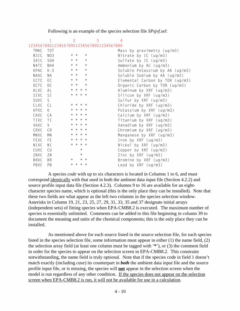
4 - 10

Following is an example of the species selection file SPsjvf.sel:

1 2 3 41234567890123456789012345678901234567890 TMAC TOT Mass by gravimetry (ug/m3) N3IC NO3 * * * Nitrate by IC (ug/m3) S4IC SO4 * * * Sulfate by IC (ug/m3) N4TC NH4 * * * Ammonium by AC (ug/m3) KPAC K-S * * * Soluble Potassium by AA (ug/m3) NAAC NA * * * Soluble Sodium by AA (ug/m3) ECTC EC * * * Elemental Carbon by TOR (ug/m3) OCTC OC * * * Organic Carbon by TOR (ug/m3) ALXC AL * * * * Aluminum by XRF (ug/m3) SIXC SI * * * * Silicon by XRF (ug/m3) SUXC S Sulfur by XRF (ug/m3) CLXC CL * * * * Chloride by XRF (ug/m3) KPXC K * * * * Potassium by XRF (ug/m3) CAXC CA * * * * Calcium by XRF (ug/m3) TIXC TI * * * * Titanium by XRF (ug/m3) VAXC V * * * * Vanadium by XRF (ug/m3) CRXC CR * * * * Chromium by XRF (ug/m3) MNXC MN * * * * Manganese by XRF (ug/m3) FEXC FE * * * * Iron by XRF (ug/m3) NIXC NI * * * * Nickel by XRF (ug/m3) CUXC CU * Copper by XRF (ug/m3) ZNXC ZN * Zinc by XRF (ug/m3) BRXC BR * * * Bromine by XRF (ug/m3) PBXC PB * * * * Lead by XRF (ug/m3)

A species code with up to six characters is located in Columns 1 to 6, and mustcorrespond identically with that used in both the ambient data input file (Section 4.2.2) andsource profile input data file (Section 4.2.3). Columns 9 to 16 are available for an eight-character species name, which is optional (this is the only place they can be installed). Note thatthese two fields are what appear as the left two columns in the species selection window. Asterisks in Column 19, 21, 23, 25, 27, 29, 31, 33, 35 and 37 designate initial arrays(independent sets) of fitting species when EPA-CMB8.2 is executed. The maximum number ofspecies is essentially unlimited. Comments can be added to this file beginning in column 39 todocument the meaning and units of the chemical components; this is the only place they can beinstalled.

As mentioned above for each source listed in the source selection file, for each specieslisted in the species selection file, some information must appear in either (1) the name field, (2)the selection array field (at least one column must be tagged with ‘*’), or (3) the comment fieldin order for the species to appear on the selection screen in EPA-CMB8.2. This constraintnotwithstanding, the name field is truly optional. Note that if the species code in field 1 doesn’tmatch exactly (including case) its counterpart in both the ambient data input file and the sourceprofile input file, or is missing, the species will not appear in the selection screen when themodel is run regardless of any other condition. If the species does not appear on the selectionscreen when EPA-CMB8.2 is run, it will not be available for use in a calculation.

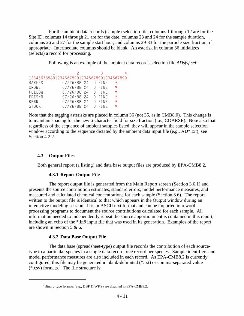
7Binary-type formats (e.g., DBF & WKS) are disabled in EPA-CMB8.2.

4 - 11

For the ambient data records (sample) selection file, columns 1 through 12 are for theSite ID, columns 14 through 21 are for the date, columns 23 and 24 for the sample duration,columns 26 and 27 for the sample start hour, and columns 29-33 for the particle size fraction, ifappropriate. Intermediate columns should be blank. An asterisk in column 36 initializes(selects) a record for processing.

Following is an example of the ambient data records selection file ADsjvf.sel:

1 2 3 412345678980123456789012345678901234567890BAKERS 07/26/88 24 0 FINE *CROWS 07/26/88 24 0 FINE *FELLOW 07/26/88 24 0 FINE *FRESNO 07/26/88 24 0 FINE * KERN 07/26/88 24 0 FINE *STOCKT 07/26/88 24 0 FINE *

Note that the tagging asterisks are placed in column 36 (not 35, as in CMB8.0). This change isto maintain spacing for the new 6-character field for size fraction (i.e., COARSE). Note also thatregardless of the sequence of ambient samples listed, they will appear in the sample selectionwindow according to the sequence dictated by the ambient data input file (e.g., AD*.txt); seeSection 4.2.2.

4.3 Output Files

Both general report (a listing) and data base output files are produced by EPA-CMB8.2.

4.3.1 Report Output File

The report output file is generated from the Main Report screen (Section 3.6.1) andpresents the source contribution estimates, standard errors, model performance measures, andmeasured and calculated chemical concentrations for each sample (Section 3.6). The reportwritten to the output file is identical to that which appears in the Output window during aninteractive modeling session. It is in ASCII text format and can be imported into wordprocessing programs to document the source contributions calculated for each sample. Allinformation needed to independently repeat the source apportionment is contained in this report,including an echo of the *.in8 input file that was used in its generation. Examples of the reportare shown in Section 5 & 6.

4.3.2 Data Base Output File

The data base (spreadsheet-type) output file records the contribution of each source-type to a particular species in a single data record, one record per species. Sample identifiers andmodel performance measures are also included in each record. As EPA-CMB8.2 is currentlyconfigured, this file may be generated in blank-delimited (*.txt) or comma-separated value(*.csv) formats.7 The file structure is:

8Fields 11 & 12 (calculated species concentration/uncertainty) are a new feature in EPA-CMB8.2 that make the outputdata file more robust.

4 - 12

Field 1: Species CodeField 2: Species NameField 3: Fitting flag; a '*' indicates a fitting species, while a '_' indicates a floating speciesField 4: Sampling site identifierField 5: Sampling dateField 6: Sample start hourField 7: Sample durationField 8: Particle size fractionField 9: Measured species concentrationField 10: Uncertainty of measured species concentrationField 11: Calculated species concentrationField 12 Uncertainty of calculated species concentrationField 13: R-square valueField 14: Chi-square valueField 15: Percent of measured massField 16+2n: Source contribution estimate, n = 0, 1, 2, ....Field 17+2n: Standard error of source contribution estimate, n = 0, 1, 2, ....

Fields 1, 2, and 4 through 8 record the sample information. Fields 3 and 11 through15 provide information about the EPA-CMB8.2 calculation.8 The remaining fields correspond toeach source profile in the PR*.* data file and contain the source contribution estimates andstandard errors for these sources. A value of -99. is recorded when a profile was not used in thecalculation.

The first record in this output file contains the field identifiers. All subsequent recordscontain data. Fields 16+2n and 17+2n are labeled with source codes and source names,respectively.

4.4 Creating Data Input Files

When using a Control File, note that if several data input files (e.g., AD*.* & PR*.*)exist for which the only difference is format, EPA-CMB8.2 assumes that the files will be namedidentically except for the extension. For blank-delimited and comma-separated value input files,there are three common methods of creating EPA-CMB8.2 input files: 1) manually entering thedata in the correct format using a text editor or word processing program; 2) editing existinginput files with a text editor or word processing program; or 3) transferring files fromcomputerized data bases.

A text editor or word processor in text mode can be used to type entire input files. It isbest to bring the example files into the editor, then insert the new values in the same locations asthe existing values by using the editor in TYPEOVER mode. Spaces between fields should beentered with the space bar; tabs should not be set. Each line should be terminated with the

4 - 13

ENTER key rather than using the wraparound feature present in many editors. No blank lines atthe end of the file should be present. Completed files should be saved with an appropriatefilename. A wide variety of very good ASCII text editors are available for creating andmanipulating input files.

When data files have been prepared for other applications (e.g., source profiles may becommon to several different data sets), these files may be cut and pasted to produce the neededinput data files. Owing to differences in individual editing programs, the user is should consultthe manual for the editing program to be used for directions on opening a copy of the existingfile, deleting and adding material, saving the changes, and renaming the file. When using wordprocessors (e.g., MSWord or WordPerfect), the files must be saved as DOS text with line breaks. Otherwise, extra information is included in the files that EPA-CMB8.2 cannot read.

Input files are most easily produced with spreadsheet or data base software. Manysource profile and ambient data sets are available in data base management formats. Selectionsof data, field names, and data structure can be easily made by the data base software. These canbe saved using the Save As or Export selections from the File menu. The CSV, DBF, and WKSformats can be selected from the “Save as type” option box that usually appears in the “Save As”window.

4.5 Reading Output Files

Main Report (ASCII) text files can be read directly into a word processing applicationwhere the detailed output for each sample can usually be displayed on a single page withcolumns aligned using a non-proportional font, e.g., a New Courier or Letter Gothic 8-point to10-point. Such a fixed pitch font in which every character occupies the same space is necessaryfor columns to be correctly aligned. As mentioned in Section 4.3.2, data base (spreadsheet-type)output files from EPA-CMB8.2 are formatted either as ASCII (default) or comma-separatedvalue (CSV), and this selection must be made on the Options screen before a calculation is made.The output file will be stored in the directory in which the Control File resides (which can, ofcourse, be changed in the browse dialog). These output files can be opened directly by data baseor spreadsheet applications, e.g., Microsoft’s Excel®, and from there exported into any of severaldifferent formats, e.g., xls. The contents of the EPA-CMB8.2 output screen can also be selectedand copied to the clipboard for pasting into other Windows® applications. Graphs made withEPA-CMB8.2 (Section 3.3 & 3.5) can be printed directly from the screen or copied to theWindows® clipboard via copy command, then pasted into a text box or frame in a wordprocessing application.

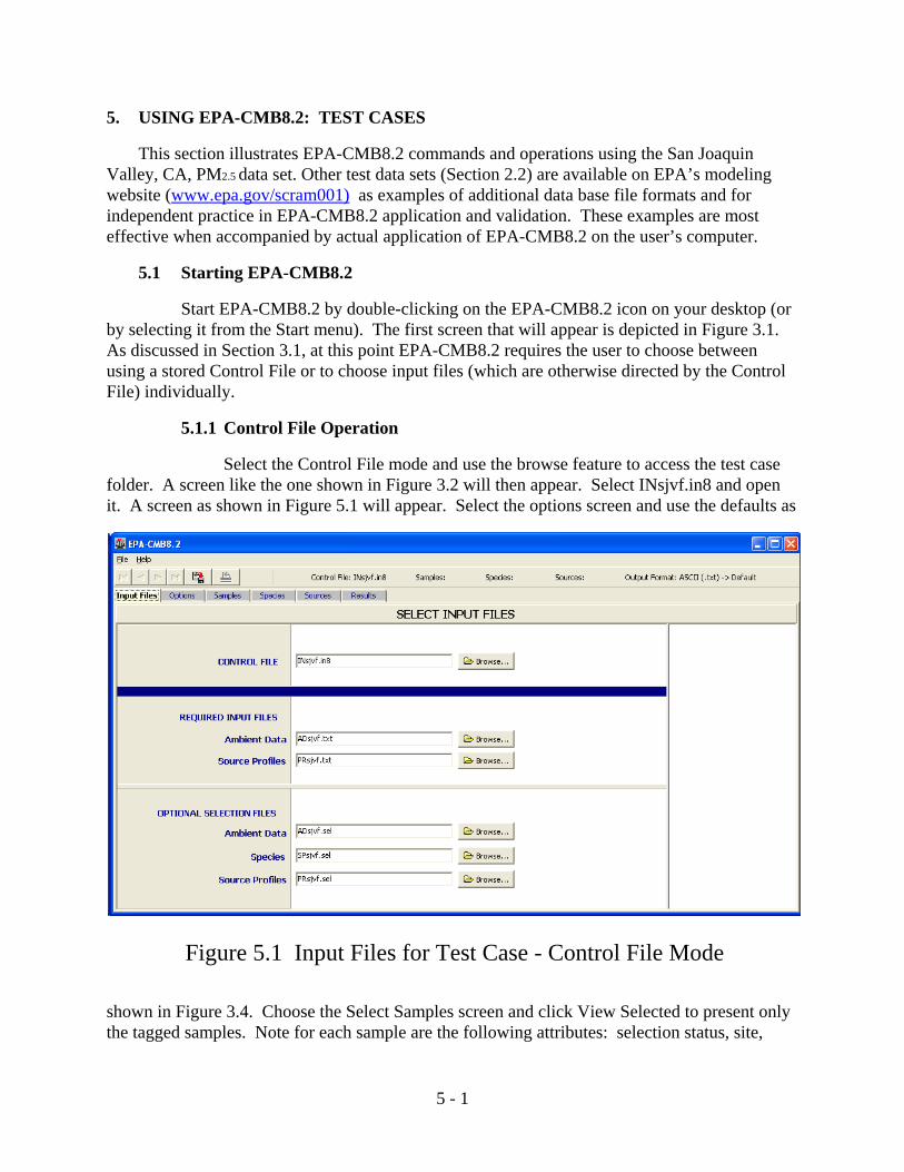
5 - 1

Figure 5.1 Input Files for Test Case - Control File Mode

5. USING EPA-CMB8.2: TEST CASES

This section illustrates EPA-CMB8.2 commands and operations using the San JoaquinValley, CA, PM2.5 data set. Other test data sets (Section 2.2) are available on EPA’s modelingwebsite (www.epa.gov/scram001) as examples of additional data base file formats and forindependent practice in EPA-CMB8.2 application and validation. These examples are mosteffective when accompanied by actual application of EPA-CMB8.2 on the user’s computer.

5.1 Starting EPA-CMB8.2

Start EPA-CMB8.2 by double-clicking on the EPA-CMB8.2 icon on your desktop (or by selecting it from the Start menu). The first screen that will appear is depicted in Figure 3.1.As discussed in Section 3.1, at this point EPA-CMB8.2 requires the user to choose betweenusing a stored Control File or to choose input files (which are otherwise directed by the ControlFile) individually.

5.1.1 Control File Operation

Select the Control File mode and use the browse feature to access the test casefolder. A screen like the one shown in Figure 3.2 will then appear. Select INsjvf.in8 and openit. A screen as shown in Figure 5.1 will appear. Select the options screen and use the defaults as

shown in Figure 3.4. Choose the Select Samples screen and click View Selected to present onlythe tagged samples. Note for each sample are the following attributes: selection status, site,

5 - 2

Figure 5.2 Ambient Samples for Test Case

sample date, sampling duration (hours), start hour, and size fraction (Figure 5.2). This isfollowed by a series of fields for measured concentration and uncertainty for total mass and forconstituent species in the sample. Measured values for species may be viewed by moving to theright through the field using the horizontal scroll, and these values may also be hidden (HideData).

Note that the “VCR” control buttons (red rectangle on toolbar) can be used to facilitatenavigation through the selection field, for purposes of selecting or de-selecting individualsamples.

Highlight any cell for the ambient sample for Fellows, CA (FELLOWS 07/26/88), as shownin Figure 5.2, and see a graphical representation of the sample (View Graph), as shown in Figure5.3. This graph may be printed from the print icon on that screen. Note that you may stepthrough the list of samples by using the “VCR” control buttons to view their graphicalrepresentations. You may then return to the Sample screen (View Grid).

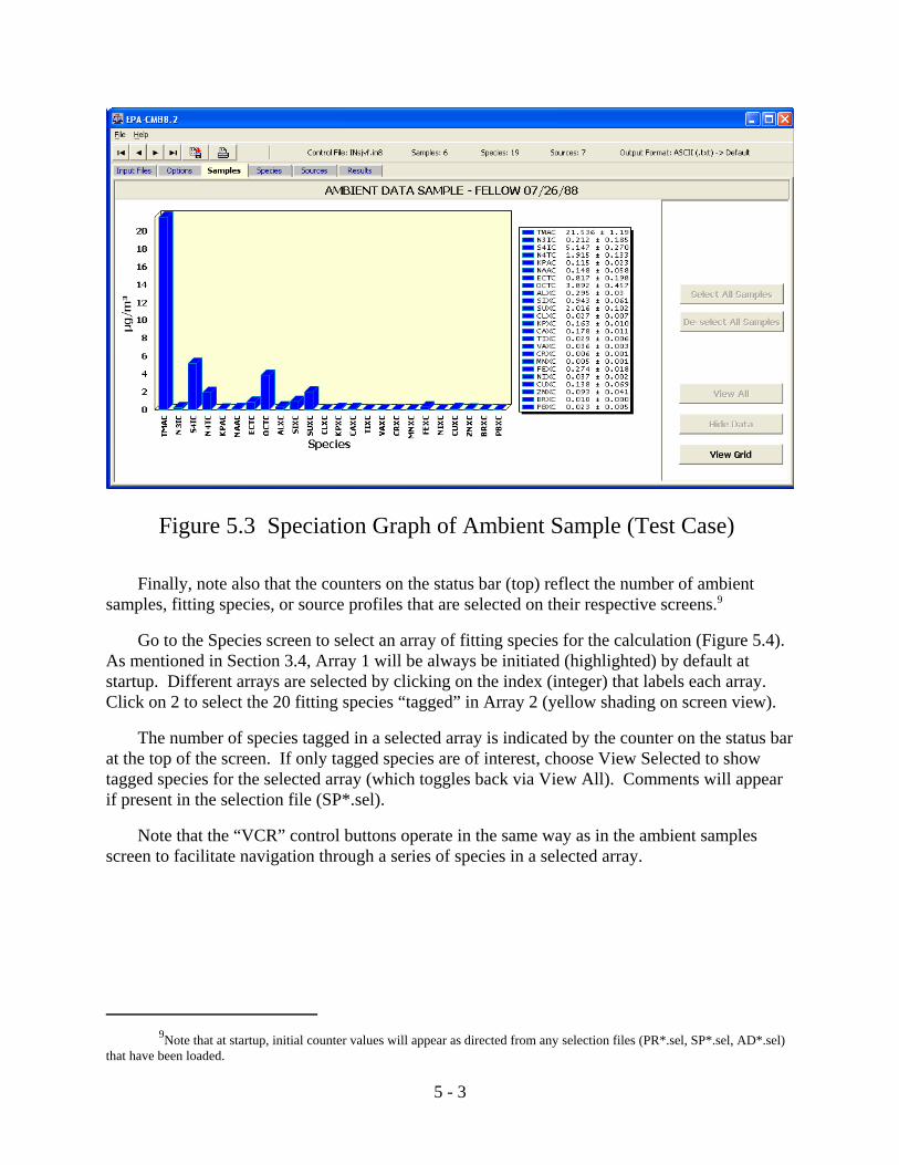
9Note that at startup, initial counter values will appear as directed from any selection files (PR*.sel, SP*.sel, AD*.sel)that have been loaded.

5 - 3

Figure 5.3 Speciation Graph of Ambient Sample (Test Case)

Finally, note also that the counters on the status bar (top) reflect the number of ambientsamples, fitting species, or source profiles that are selected on their respective screens.9

Go to the Species screen to select an array of fitting species for the calculation (Figure 5.4). As mentioned in Section 3.4, Array 1 will be always be initiated (highlighted) by default atstartup. Different arrays are selected by clicking on the index (integer) that labels each array. Click on 2 to select the 20 fitting species “tagged” in Array 2 (yellow shading on screen view).

The number of species tagged in a selected array is indicated by the counter on the status barat the top of the screen. If only tagged species are of interest, choose View Selected to showtagged species for the selected array (which toggles back via View All). Comments will appearif present in the selection file (SP*.sel).

Note that the “VCR” control buttons operate in the same way as in the ambient samplesscreen to facilitate navigation through a series of species in a selected array.

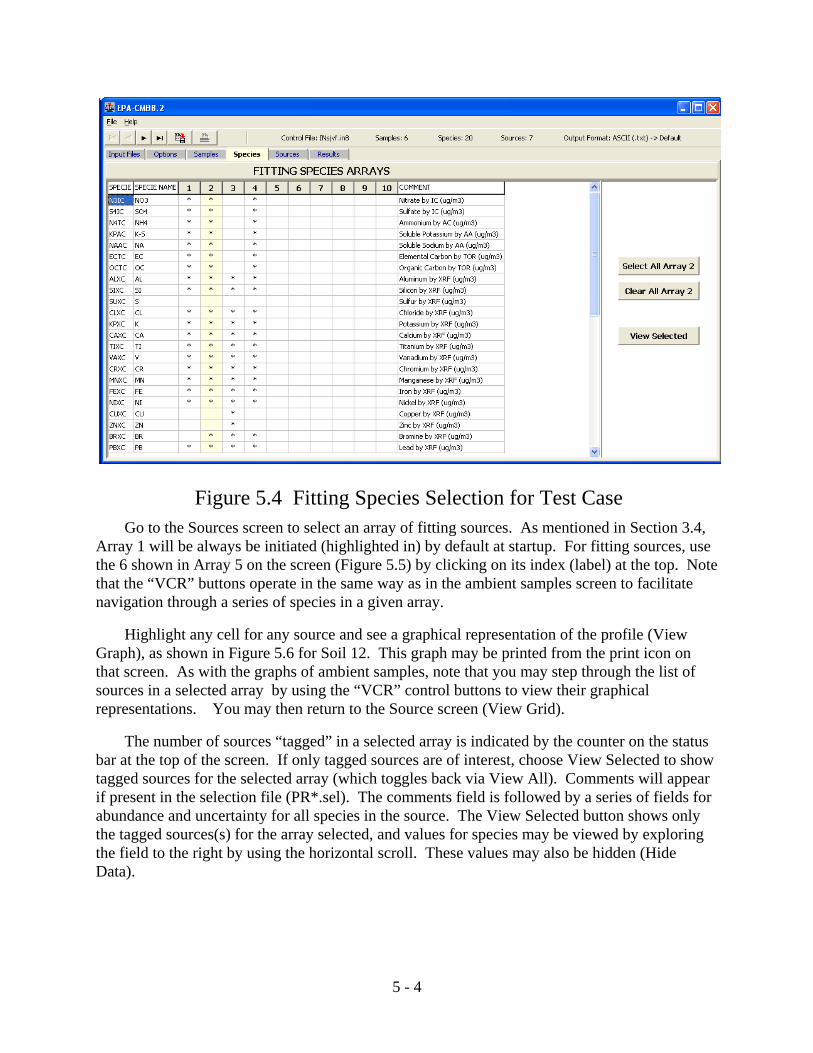
5 - 4

Figure 5.4 Fitting Species Selection for Test CaseGo to the Sources screen to select an array of fitting sources. As mentioned in Section 3.4,

Array 1 will be always be initiated (highlighted in) by default at startup. For fitting sources, usethe 6 shown in Array 5 on the screen (Figure 5.5) by clicking on its index (label) at the top. Notethat the “VCR” buttons operate in the same way as in the ambient samples screen to facilitatenavigation through a series of species in a given array.

Highlight any cell for any source and see a graphical representation of the profile (ViewGraph), as shown in Figure 5.6 for Soil 12. This graph may be printed from the print icon onthat screen. As with the graphs of ambient samples, note that you may step through the list ofsources in a selected array by using the “VCR” control buttons to view their graphicalrepresentations. You may then return to the Source screen (View Grid).

The number of sources “tagged” in a selected array is indicated by the counter on the statusbar at the top of the screen. If only tagged sources are of interest, choose View Selected to showtagged sources for the selected array (which toggles back via View All). Comments will appearif present in the selection file (PR*.sel). The comments field is followed by a series of fields forabundance and uncertainty for all species in the source. The View Selected button shows onlythe tagged sources(s) for the array selected, and values for species may be viewed by exploringthe field to the right by using the horizontal scroll. These values may also be hidden (HideData).

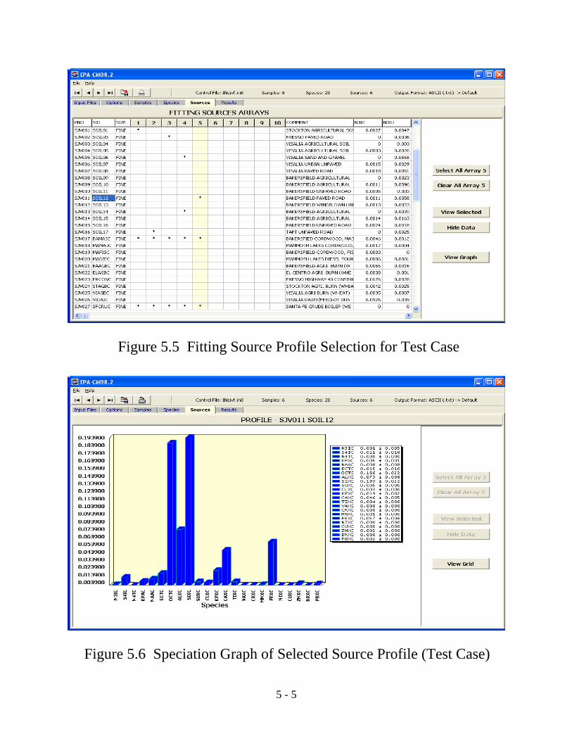
5 - 5

Figure 5.5 Fitting Source Profile Selection for Test Case

Figure 5.6 Speciation Graph of Selected Source Profile (Test Case)

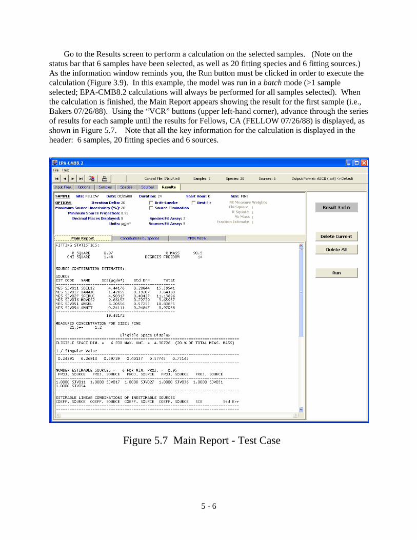
5 - 6

Figure 5.7 Main Report - Test Case

Go to the Results screen to perform a calculation on the selected samples. (Note on thestatus bar that 6 samples have been selected, as well as 20 fitting species and 6 fitting sources.) As the information window reminds you, the Run button must be clicked in order to execute thecalculation (Figure 3.9). In this example, the model was run in a batch mode (>1 sampleselected; EPA-CMB8.2 calculations will always be performed for all samples selected). Whenthe calculation is finished, the Main Report appears showing the result for the first sample (i.e.,Bakers 07/26/88). Using the “VCR” buttons (upper left-hand corner), advance through the seriesof results for each sample until the results for Fellows, CA (FELLOW 07/26/88) is displayed, asshown in Figure 5.7. Note that all the key information for the calculation is displayed in theheader: 6 samples, 20 fitting species and 6 sources.

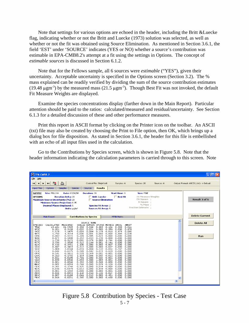
5 - 7 Figure 5.8 Contribution by Species - Test Case

Note that settings for various options are echoed in the header, including the Britt &Lueckeflag, indicating whether or not the Britt and Luecke (1973) solution was selected, as well aswhether or not the fit was obtained using Source Elimination. As mentioned in Section 3.6.1, thefield ‘EST’ under ‘SOURCE’ indicates (YES or NO) whether a source’s contribution wasestimable in EPA-CMB8.2's attempt at a fit using the settings in Options. The concept ofestimable sources is discussed in Section 6.1.2.

Note that for the Fellows sample, all 6 sources were estimable (“YES”), given theiruncertainty. Acceptable uncertainty is specified in the Options screen (Section 3.2). The %mass explained can be readily verified by dividing the sum of the source contribution estimates(19.48 :gm-3) by the measured mass (21.5 :gm-3). Though Best Fit was not invoked, the defaultFit Measure Weights are displayed.

Examine the species concentrations display (farther down in the Main Report). Particularattention should be paid to the ratios: calculated/measured and residual/uncertainty. See Section6.1.3 for a detailed discussion of these and other performance measures.

Print this report in ASCII format by clicking on the Printer icon on the toolbar. An ASCII(txt) file may also be created by choosing the Print to File option, then OK, which brings up adialog box for file disposition. As stated in Section 3.6.1, the header for this file is embellishedwith an echo of all input files used in the calculation.

Go to the Contributions by Species screen, which is shown in Figure 5.8. Note that theheader information indicating the calculation parameters is carried through to this screen. Note

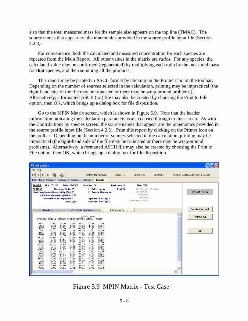
5 - 8

Figure 5.9 MPIN Matrix - Test Case

also that the total measured mass for the sample also appears on the top line (TMAC). Thesource names that appear are the mnemonics provided in the source profile input file (Section4.2.3).

For convenience, both the calculated and measured concentration for each species arerepeated from the Main Report. All other values in the matrix are ratios. For any species, thecalculated value may be confirmed (regenerated) by multiplying each ratio by the measured massfor that species, and then summing all the products.

This report may be printed in ASCII format by clicking on the Printer icon on the toolbar. Depending on the number of sources selected in the calculation, printing may be impractical (theright-hand side of the file may be truncated or there may be wrap-around problems). Alternatively, a formatted ASCII (txt) file may also be created by choosing the Print to Fileoption, then OK, which brings up a dialog box for file disposition.

Go to the MPIN Matrix screen, which is shown in Figure 5.9. Note that the headerinformation indicating the calculation parameters is also carried through to this screen. As withthe Contributions by species screen, the source names that appear are the mnemonics provided inthe source profile input file (Section 4.2.3). Print this report by clicking on the Printer icon onthe toolbar. Depending on the number of sources selected in the calculation, printing may beimpractical (the right-hand side of the file may be truncated or there may be wrap-aroundproblems). Alternatively, a formatted ASCII file may also be created by choosing the Print toFile option, then OK, which brings up a dialog box for file disposition.

5 - 9

Once satisfied with the results, the output from EPA-CMB8.2 may be exported by clickingon the File icon, then using the Save Results dialog. As discussed in Section 4.5, the outputformat will be as selected in Options (default is ASCII).

The output file is a spreadsheet-type format and contains the contribution of each source toeach measured species in each sample (Section 4.3.2). Fitting species are identified by anasterisk in the third column, and performance measures follow. Source contribution estimatesand their standard errors are presented in subsequent columns, identified by mnemonics in thefirst row. Contributions from non-fitting profiles for a sample are identified as –99. Commonspreadsheet data analysis tools can be used to interrogate files and select records for differentchemical species, to group contributions from different profiles representing the same sourcetype, to calculate average contributions, and to plot results

Close down EPA-CMB8.2 before moving on to the next exercise.

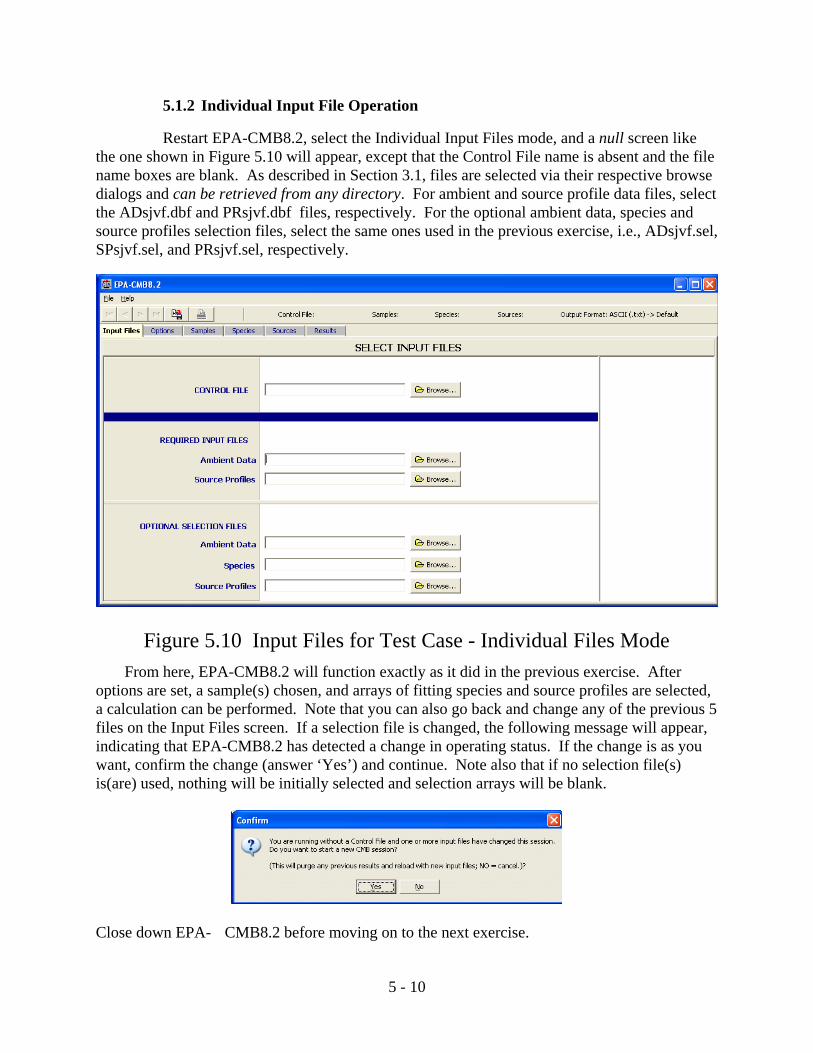
5 - 10

Figure 5.10 Input Files for Test Case - Individual Files Mode

5.1.2 Individual Input File Operation

Restart EPA-CMB8.2, select the Individual Input Files mode, and a null screen likethe one shown in Figure 5.10 will appear, except that the Control File name is absent and the filename boxes are blank. As described in Section 3.1, files are selected via their respective browsedialogs and can be retrieved from any directory. For ambient and source profile data files, selectthe ADsjvf.dbf and PRsjvf.dbf files, respectively. For the optional ambient data, species andsource profiles selection files, select the same ones used in the previous exercise, i.e., ADsjvf.sel,SPsjvf.sel, and PRsjvf.sel, respectively.

From here, EPA-CMB8.2 will function exactly as it did in the previous exercise. Afteroptions are set, a sample(s) chosen, and arrays of fitting species and source profiles are selected,a calculation can be performed. Note that you can also go back and change any of the previous 5files on the Input Files screen. If a selection file is changed, the following message will appear,indicating that EPA-CMB8.2 has detected a change in operating status. If the change is as youwant, confirm the change (answer ‘Yes’) and continue. Note also that if no selection file(s)is(are) used, nothing will be initially selected and selection arrays will be blank.

Close down EPA- CMB8.2 before moving on to the next exercise.

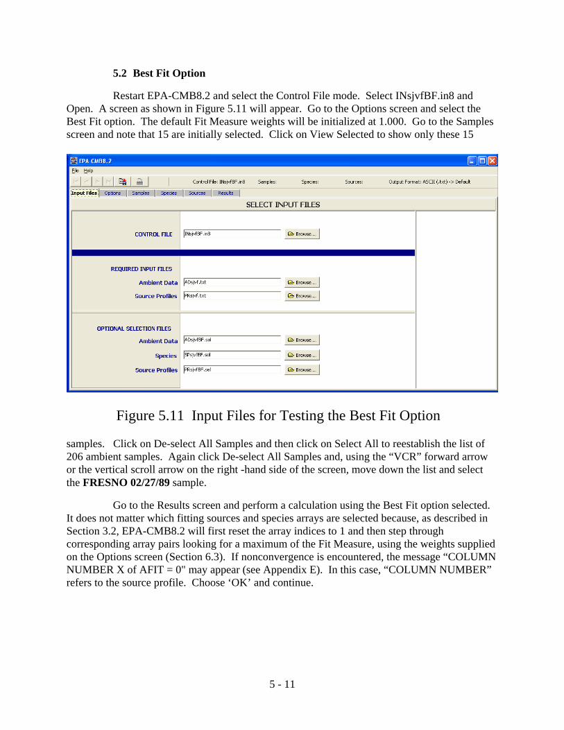
5 - 11

Figure 5.11 Input Files for Testing the Best Fit Option

5.2 Best Fit Option

Restart EPA-CMB8.2 and select the Control File mode. Select INsjvfBF.in8 andOpen. A screen as shown in Figure 5.11 will appear. Go to the Options screen and select theBest Fit option. The default Fit Measure weights will be initialized at 1.000. Go to the Samplesscreen and note that 15 are initially selected. Click on View Selected to show only these 15

samples. Click on De-select All Samples and then click on Select All to reestablish the list of206 ambient samples. Again click De-select All Samples and, using the “VCR” forward arrowor the vertical scroll arrow on the right -hand side of the screen, move down the list and selectthe FRESNO 02/27/89 sample.

Go to the Results screen and perform a calculation using the Best Fit option selected. It does not matter which fitting sources and species arrays are selected because, as described inSection 3.2, EPA-CMB8.2 will first reset the array indices to 1 and then step throughcorresponding array pairs looking for a maximum of the Fit Measure, using the weights suppliedon the Options screen (Section 6.3). If nonconvergence is encountered, the message “COLUMNNUMBER X of AFIT = 0" may appear (see Appendix E). In this case, “COLUMN NUMBER”refers to the source profile. Choose ‘OK’ and continue.

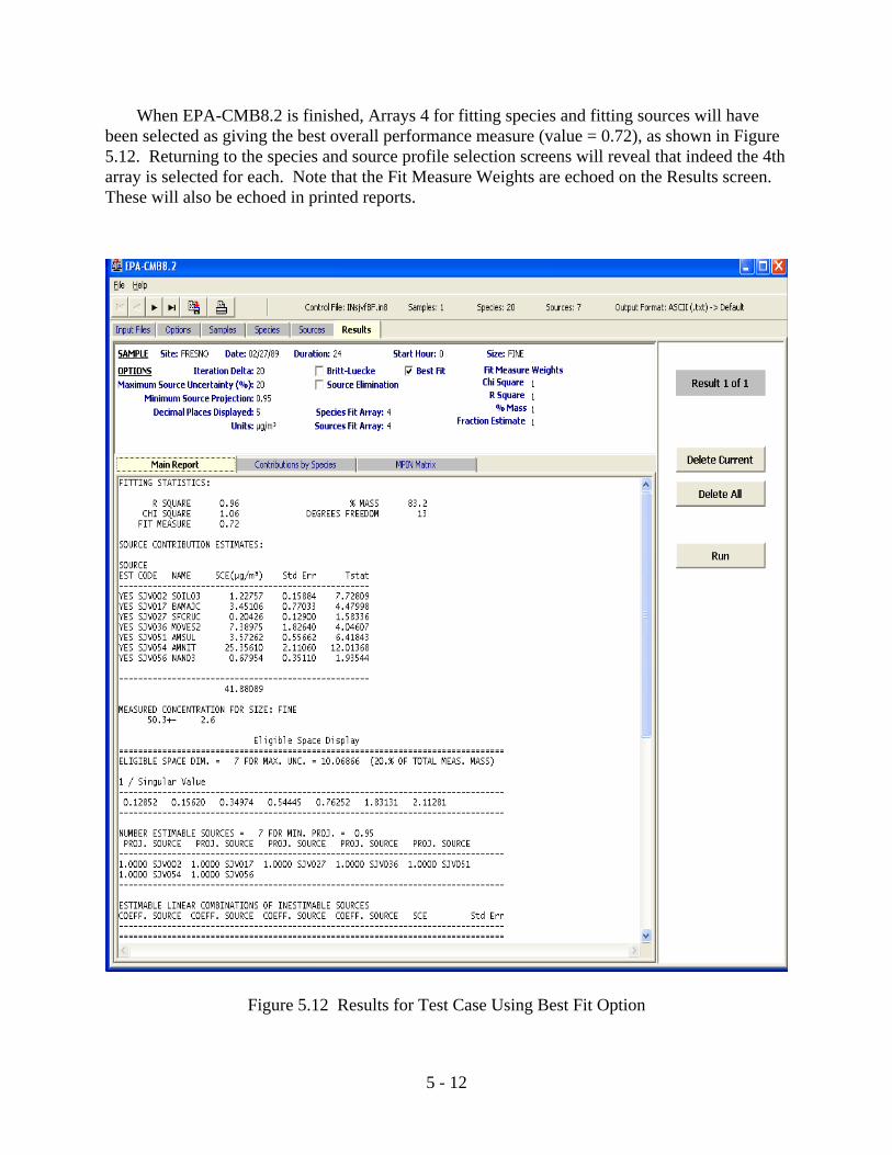
5 - 12

Figure 5.12 Results for Test Case Using Best Fit Option

When EPA-CMB8.2 is finished, Arrays 4 for fitting species and fitting sources will havebeen selected as giving the best overall performance measure (value = 0.72), as shown in Figure5.12. Returning to the species and source profile selection screens will reveal that indeed the 4tharray is selected for each. Note that the Fit Measure Weights are echoed on the Results screen. These will also be echoed in printed reports.

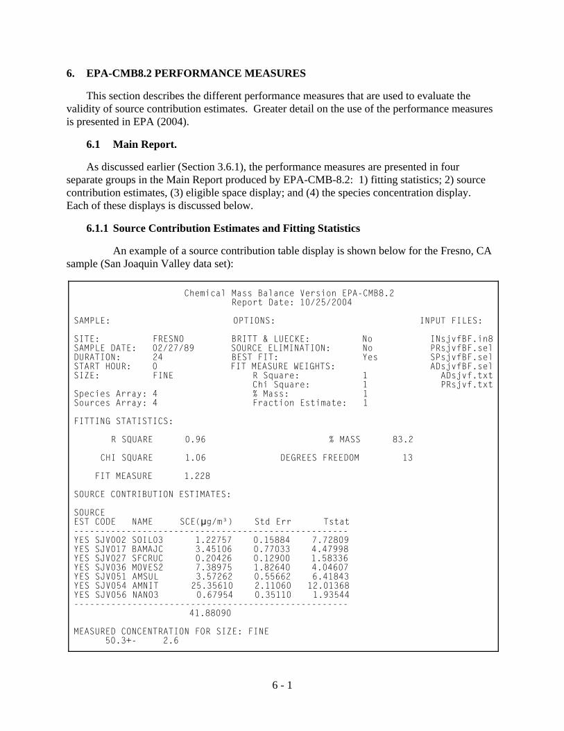
6 - 1

Chemical Mass Balance Version EPA-CMB8.2 Report Date: 10/25/2004 SAMPLE: OPTIONS: INPUT FILES: SITE: FRESNO BRITT & LUECKE: No INsjvfBF.in8SAMPLE DATE: 02/27/89 SOURCE ELIMINATION: No PRsjvfBF.selDURATION: 24 BEST FIT: Yes SPsjvfBF.selSTART HOUR: 0 FIT MEASURE WEIGHTS: ADsjvfBF.selSIZE: FINE R Square: 1 ADsjvf.txt Chi Square: 1 PRsjvf.txtSpecies Array: 4 % Mass: 1 Sources Array: 4 Fraction Estimate: 1 FITTING STATISTICS: R SQUARE 0.96 % MASS 83.2 CHI SQUARE 1.06 DEGREES FREEDOM 13 FIT MEASURE 1.228 SOURCE CONTRIBUTION ESTIMATES: SOURCE EST CODE NAME SCE(:g/m³) Std Err Tstat ---------------------------------------------------- YES SJV002 SOIL03 1.22757 0.15884 7.72809 YES SJV017 BAMAJC 3.45106 0.77033 4.47998 YES SJV027 SFCRUC 0.20426 0.12900 1.58336 YES SJV036 MOVES2 7.38975 1.82640 4.04607 YES SJV051 AMSUL 3.57262 0.55662 6.41843 YES SJV054 AMNIT 25.35610 2.11060 12.01368 YES SJV056 NANO3 0.67954 0.35110 1.93544 ---------------------------------------------------- 41.88090 MEASURED CONCENTRATION FOR SIZE: FINE 50.3+- 2.6

6. EPA-CMB8.2 PERFORMANCE MEASURES

This section describes the different performance measures that are used to evaluate thevalidity of source contribution estimates. Greater detail on the use of the performance measuresis presented in EPA (2004).

6.1 Main Report.

As discussed earlier (Section 3.6.1), the performance measures are presented in fourseparate groups in the Main Report produced by EPA-CMB-8.2: 1) fitting statistics; 2) sourcecontribution estimates, (3) eligible space display; and (4) the species concentration display. Each of these displays is discussed below.

6.1.1 Source Contribution Estimates and Fitting Statistics

An example of a source contribution table display is shown below for the Fresno, CAsample (San Joaquin Valley data set):

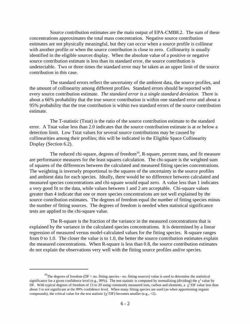
10The degrees of freedom (DF = no. fitting species - no. fitting sources) value is used to determine the statisticalsignificance for a given confidence level (e.g., 99%). The test statistic is computed by normalizing (dividing) the P2 value byDF. With typical degrees of freedom of 13 to 20 using commonly measured ions, carbon and elements, a P2/DF value less thanabout 3 is not significant at the 99% confidence level. When many fitting species are used (as when apportioning organiccompounds), the critical value for the test statistic (P2/DF) becomes smaller (e.g., <2).

6 - 2

Source contribution estimates are the main output of EPA-CMB8.2. The sum of theseconcentrations approximates the total mass concentration. Negative source contributionestimates are not physically meaningful, but they can occur when a source profile is collinearwith another profile or when the source contribution is close to zero. Collinearity is usuallyidentified in the eligible sources display. When the absolute value of a positive or negativesource contribution estimate is less than its standard error, the source contribution isundetectable. Two or three times the standard error may be taken as an upper limit of the sourcecontribution in this case.

The standard errors reflect the uncertainty of the ambient data, the source profiles, andthe amount of collinearity among different profiles. Standard errors should be reported withevery source contribution estimate. The standard error is a single standard deviation. There isabout a 66% probability that the true source contribution is within one standard error and about a95% probability that the true contribution is within two standard errors of the source contributionestimate.

The T-statistic (Tstat) is the ratio of the source contribution estimate to the standarderror. A Tstat value less than 2.0 indicates that the source contribution estimate is at or below adetection limit. Low Tstat values for several source contributions may be caused bycollinearities among their profiles; this will be indicated in the Eligible Space CollinearityDisplay (Section 6.2).

The reduced chi-square, degrees of freedom10, R-square, percent mass, and fit measureare performance measures for the least squares calculation. The chi-square is the weighted sumof squares of the differences between the calculated and measured fitting species concentrations. The weighting is inversely proportional to the squares of the uncertainty in the source profilesand ambient data for each species. Ideally, there would be no difference between calculated andmeasured species concentrations and chi-square would equal zero. A value less than 1 indicatesa very good fit to the data, while values between 1 and 2 are acceptable. Chi-square valuesgreater than 4 indicate that one or more species concentrations are not well explained by thesource contribution estimates. The degrees of freedom equal the number of fitting species minusthe number of fitting sources. The degrees of freedom is needed when statistical significancetests are applied to the chi-square value.

The R-square is the fraction of the variance in the measured concentrations that isexplained by the variance in the calculated species concentrations. It is determined by a linearregression of measured versus model-calculated values for the fitting species. R-square rangesfrom 0 to 1.0. The closer the value is to 1.0, the better the source contribution estimates explainthe measured concentrations. When R-square is less than 0.8, the source contribution estimatesdo not explain the observations very well with the fitting source profiles and/or species.

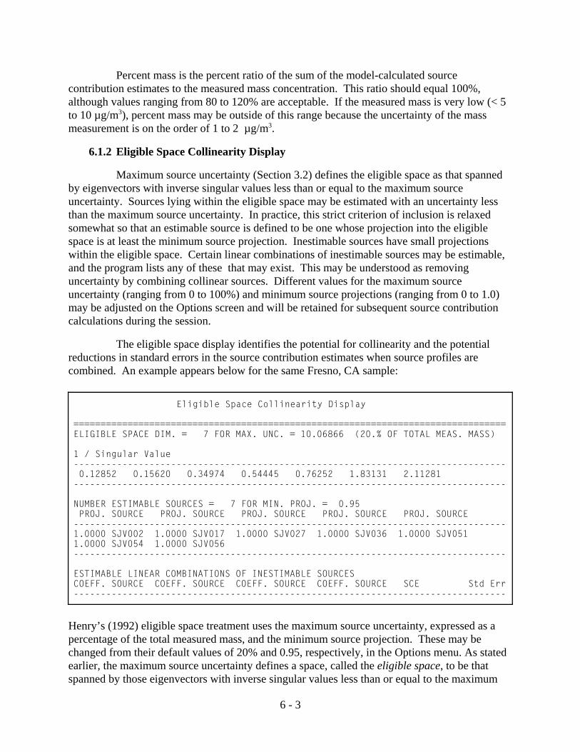
6 - 3

Eligible Space Collinearity Display

================================================================================ELIGIBLE SPACE DIM. = 7 FOR MAX. UNC. = 10.06866 (20.% OF TOTAL MEAS. MASS) 1 / Singular Value -------------------------------------------------------------------------------- 0.12852 0.15620 0.34974 0.54445 0.76252 1.83131 2.11281 -------------------------------------------------------------------------------- NUMBER ESTIMABLE SOURCES = 7 FOR MIN. PROJ. = 0.95 PROJ. SOURCE PROJ. SOURCE PROJ. SOURCE PROJ. SOURCE PROJ. SOURCE --------------------------------------------------------------------------------1.0000 SJV002 1.0000 SJV017 1.0000 SJV027 1.0000 SJV036 1.0000 SJV051 1.0000 SJV054 1.0000 SJV056 -------------------------------------------------------------------------------- ESTIMABLE LINEAR COMBINATIONS OF INESTIMABLE SOURCES COEFF. SOURCE COEFF. SOURCE COEFF. SOURCE COEFF. SOURCE SCE Std Err--------------------------------------------------------------------------------

Percent mass is the percent ratio of the sum of the model-calculated sourcecontribution estimates to the measured mass concentration. This ratio should equal 100%,although values ranging from 80 to 120% are acceptable. If the measured mass is very low (< 5to 10 µg/m3), percent mass may be outside of this range because the uncertainty of the massmeasurement is on the order of 1 to 2 µg/m3.

6.1.2 Eligible Space Collinearity Display

Maximum source uncertainty (Section 3.2) defines the eligible space as that spannedby eigenvectors with inverse singular values less than or equal to the maximum sourceuncertainty. Sources lying within the eligible space may be estimated with an uncertainty lessthan the maximum source uncertainty. In practice, this strict criterion of inclusion is relaxedsomewhat so that an estimable source is defined to be one whose projection into the eligiblespace is at least the minimum source projection. Inestimable sources have small projectionswithin the eligible space. Certain linear combinations of inestimable sources may be estimable,and the program lists any of these that may exist. This may be understood as removinguncertainty by combining collinear sources. Different values for the maximum sourceuncertainty (ranging from 0 to 100%) and minimum source projections (ranging from 0 to 1.0)may be adjusted on the Options screen and will be retained for subsequent source contributioncalculations during the session.

The eligible space display identifies the potential for collinearity and the potentialreductions in standard errors in the source contribution estimates when source profiles arecombined. An example appears below for the same Fresno, CA sample:

Henry’s (1992) eligible space treatment uses the maximum source uncertainty, expressed as apercentage of the total measured mass, and the minimum source projection. These may bechanged from their default values of 20% and 0.95, respectively, in the Options menu. As statedearlier, the maximum source uncertainty defines a space, called the eligible space, to be thatspanned by those eigenvectors with inverse singular values less than or equal to the maximum

6 - 4

source uncertainty. The first part of this display gives the eligible space dimension and theuncertainty used in its calculation. This is followed by a listing of the inverse singular values.

It was mentioned in Section 1.1 that EPA-CMB8.2 gives the user control in adjusting collinearity parameters which in CMB7 are "hard-wired" and not necessarily optimum for everyapplication. Historically these parameters were chosen in CMB7 to be compatible withcharacteristics of particulate mass measurements, particularly those made by X-ray fluorescence. On an absolute basis with different measurement units, uncertainties associated with VOC maybe up to an order of magnitude lower than those for particles. In an effort to resolve thisdiscrepancy, the maximum source uncertainty (threshold set in Options; Section 3.2) in EPA-CMB8.2 is expressed as a percentage (“unit neutral”).

The next part of the display gives the number of estimable sources, the minimumsource projection used in the calculation, and the projections of each profile vector into theeligible space. Inestimable sources are caused by excessive similarity (collinearity) among thesource profiles or by high uncertainties in the individual source profiles. The standard errorsassociated with the source contribution estimates of one or more inestimable sources are usuallyvery large, often too large to allow an adequate separation of these source contributions to bemade. Inestimable sources will not appear if the two above-stated conditions (i.e., collinearity orlarge std. error of the SCE) do not occur. An absence of inestimable sources means that thesource contributions can be resolved in the specific application. Since ambient datauncertainties, and relative levels of source contributions, vary from sample to sample, it ispossible that a given set of profiles may appear in the ineligible (inestimable) space for one set ofambient data, but not for another set. For this reason, it is impossible to decide a priori that a setof profiles is collinear or not. The decision must be made for each set of data and each set ofprofiles combined with those data.

If collinearity is the cause of these excessive standard errors, then certain linearcombinations of inestimable sources may be estimable, and the final part of the display liststhese, if any exist. This may be understood as removing uncertainty by combining collinearsources. This linear combination may be more useful than the individual source contributionestimates if the standard error of the linear combination is substantially lower than the standarderrors of each source contribution estimate. However, the treatment does not allowdifferentiation among the contribution estimates of the sources contained in the linearcombination. Also, as stated above for the individual source data, the number of decimal placesused in the presentation of the inverse singular values is that set in the Options menu. For morediscussion of collinearity, see Section 4.1 of EPA, 2004.

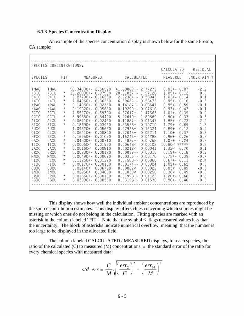
6 - 5

================================================================================SPECIES CONCENTRATIONS: CALCULATED RESIDUAL ---------- -----------SPECIES FIT MEASURED CALCULATED MEASURED UNCERTAINTY-------------------------------------------------------------------------------- TMAC TMAU 50.34330+- 2.56520 41.88089+- 2.77273 0.83+- 0.07 -2.2 N3IC N3IU * 19.26080+- 0.97930 20.31037+- 1.97128 1.05+- 0.12 0.5 S4IC S4IU * 2.87790+- 0.16530 2.92384+- 0.36943 1.02+- 0.14 0.1 N4TC N4TU * 7.04960+- 0.36360 6.69662+- 0.58473 0.95+- 0.10 -0.5 KPAC KPAU * 0.14960+- 0.02350 0.14187+- 0.08541 0.95+- 0.59 -0.1 NAAC NAAU * 0.19820+- 0.05660 0.19290+- 0.07618 0.97+- 0.47 -0.1 ECTC ECTU * 4.55270+- 0.59790 4.57617+- 1.47563 1.01+- 0.35 0.0 OCTC OCTU * 5.99850+- 0.84490 5.42610+- 1.80669 0.90+- 0.33 -0.3 ALXC ALXU * 0.06410+- 0.02420 0.11887+- 0.01347 1.85+- 0.73 2.0 SIXC SIXU * 0.18690+- 0.03920 0.33528+- 0.10710 1.79+- 0.69 1.3 SUXC SUXU 1.09520+- 0.05650 0.97978+- 0.12324 0.89+- 0.12 -0.9 CLXC CLXU * 0.06410+- 0.00800 0.07043+- 0.02214 1.10+- 0.37 0.3 KPXC KPXU * 0.16950+- 0.01070 0.16243+- 0.04288 0.96+- 0.26 -0.2 CAXC CAXU * 0.04500+- 0.00710 0.04837+- 0.00768 1.07+- 0.24 0.3 TIXC TIXU * 0.00060< 0.01930 0.00648< 0.00103 10.80< ***** 0.3 VAXC VAXU * 0.00160< 0.00810 0.00212< 0.00041 1.32< 6.70 0.1 CRXC CRXU * 0.00200+- 0.00170 0.00039+- 0.00015 0.19+- 0.18 -0.9 MNXC MNXU * 0.00490+- 0.00090 0.00356+- 0.00178 0.73+- 0.39 -0.7 FEXC FEXU * 0.11250+- 0.01290 0.07588+- 0.00860 0.67+- 0.11 -2.4 NIXC NIXU * 0.00170+- 0.00100 0.00174+- 0.00024 1.02+- 0.62 0.0 CUXC CUXU 0.02140< 0.06790 0.00062< 0.00022 0.03< 0.09 -0.3 ZNXC ZNXU 0.02950< 0.04030 0.01050< 0.00250 0.36< 0.49 -0.5 BRXC BRXU * 0.01660+- 0.00100 0.01998+- 0.01123 1.20+- 0.68 0.3 PBXC PBXU * 0.03990+- 0.00560 0.03198+- 0.01530 0.80+- 0.40 -0.5 --------------------------------------------------------------------------------

6.1.3 Species Concentration Display

An example of the species concentration display is shown below for the same Fresno,CA sample:

This display shows how well the individual ambient concentrations are reproduced bythe source contribution estimates. This display offers clues concerning which sources might bemissing or which ones do not belong in the calculation. Fitting species are marked with anasterisk in the column labeled ' FIT '. Note that the symbol < flags measured values less thanthe uncertainty. The block of asterisks indicate numerical overflow, meaning that the number istoo large to be displayed in the allocated field.

The column labeled CALCULATED / MEASURED displays, for each species, theratio of the calculated (C) to measured (M) concentrations ± the standard error of the ratio forevery chemical species with measured data:

std errCM

errC

errM

C M. =⎛⎝⎜

⎞⎠⎟ +

⎛⎝⎜

⎞⎠⎟

2 2

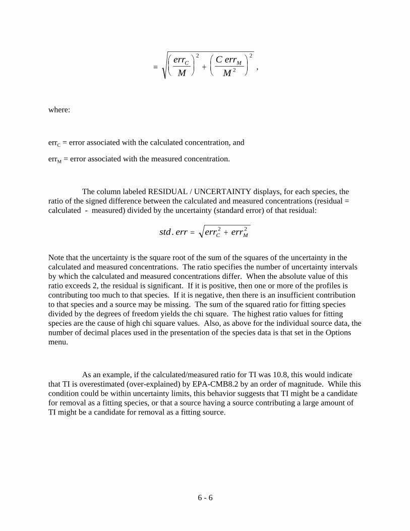
6 - 6

,=⎛⎝⎜

⎞⎠⎟ +

⎛⎝⎜

⎞⎠⎟

errM

C errM

C M2

2

2

where:

errC = error associated with the calculated concentration, and

errM = error associated with the measured concentration.

The column labeled RESIDUAL / UNCERTAINTY displays, for each species, theratio of the signed difference between the calculated and measured concentrations (residual =calculated - measured) divided by the uncertainty (standard error) of that residual:

std err err errC M. = +2 2

Note that the uncertainty is the square root of the sum of the squares of the uncertainty in thecalculated and measured concentrations. The ratio specifies the number of uncertainty intervalsby which the calculated and measured concentrations differ. When the absolute value of thisratio exceeds 2, the residual is significant. If it is positive, then one or more of the profiles iscontributing too much to that species. If it is negative, then there is an insufficient contributionto that species and a source may be missing. The sum of the squared ratio for fitting speciesdivided by the degrees of freedom yields the chi square. The highest ratio values for fittingspecies are the cause of high chi square values. Also, as above for the individual source data, thenumber of decimal places used in the presentation of the species data is that set in the Optionsmenu.

As an example, if the calculated/measured ratio for TI was 10.8, this would indicatethat TI is overestimated (over-explained) by EPA-CMB8.2 by an order of magnitude. While thiscondition could be within uncertainty limits, this behavior suggests that TI might be a candidatefor removal as a fitting species, or that a source having a source contributing a large amount ofTI might be a candidate for removal as a fitting source.

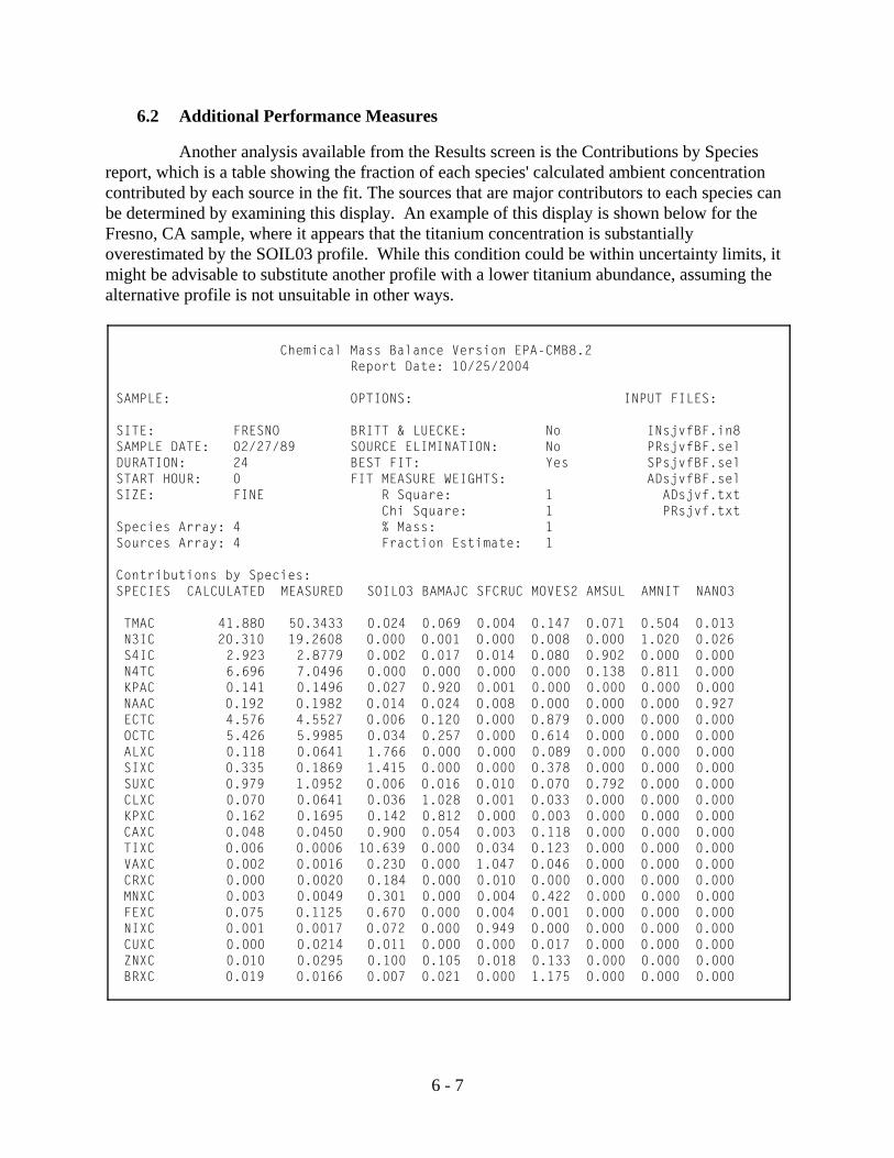
6 - 7

Chemical Mass Balance Version EPA-CMB8.2 Report Date: 10/25/2004 SAMPLE: OPTIONS: INPUT FILES: SITE: FRESNO BRITT & LUECKE: No INsjvfBF.in8SAMPLE DATE: 02/27/89 SOURCE ELIMINATION: No PRsjvfBF.selDURATION: 24 BEST FIT: Yes SPsjvfBF.selSTART HOUR: 0 FIT MEASURE WEIGHTS: ADsjvfBF.selSIZE: FINE R Square: 1 ADsjvf.txt Chi Square: 1 PRsjvf.txtSpecies Array: 4 % Mass: 1 Sources Array: 4 Fraction Estimate: 1 Contributions by Species: SPECIES CALCULATED MEASURED SOIL03 BAMAJC SFCRUC MOVES2 AMSUL AMNIT NANO3

TMAC 41.880 50.3433 0.024 0.069 0.004 0.147 0.071 0.504 0.013 N3IC 20.310 19.2608 0.000 0.001 0.000 0.008 0.000 1.020 0.026 S4IC 2.923 2.8779 0.002 0.017 0.014 0.080 0.902 0.000 0.000 N4TC 6.696 7.0496 0.000 0.000 0.000 0.000 0.138 0.811 0.000 KPAC 0.141 0.1496 0.027 0.920 0.001 0.000 0.000 0.000 0.000 NAAC 0.192 0.1982 0.014 0.024 0.008 0.000 0.000 0.000 0.927 ECTC 4.576 4.5527 0.006 0.120 0.000 0.879 0.000 0.000 0.000 OCTC 5.426 5.9985 0.034 0.257 0.000 0.614 0.000 0.000 0.000 ALXC 0.118 0.0641 1.766 0.000 0.000 0.089 0.000 0.000 0.000 SIXC 0.335 0.1869 1.415 0.000 0.000 0.378 0.000 0.000 0.000 SUXC 0.979 1.0952 0.006 0.016 0.010 0.070 0.792 0.000 0.000 CLXC 0.070 0.0641 0.036 1.028 0.001 0.033 0.000 0.000 0.000 KPXC 0.162 0.1695 0.142 0.812 0.000 0.003 0.000 0.000 0.000 CAXC 0.048 0.0450 0.900 0.054 0.003 0.118 0.000 0.000 0.000 TIXC 0.006 0.0006 10.639 0.000 0.034 0.123 0.000 0.000 0.000 VAXC 0.002 0.0016 0.230 0.000 1.047 0.046 0.000 0.000 0.000 CRXC 0.000 0.0020 0.184 0.000 0.010 0.000 0.000 0.000 0.000 MNXC 0.003 0.0049 0.301 0.000 0.004 0.422 0.000 0.000 0.000 FEXC 0.075 0.1125 0.670 0.000 0.004 0.001 0.000 0.000 0.000 NIXC 0.001 0.0017 0.072 0.000 0.949 0.000 0.000 0.000 0.000 CUXC 0.000 0.0214 0.011 0.000 0.000 0.017 0.000 0.000 0.000 ZNXC 0.010 0.0295 0.100 0.105 0.018 0.133 0.000 0.000 0.000 BRXC 0.019 0.0166 0.007 0.021 0.000 1.175 0.000 0.000 0.000

6.2 Additional Performance Measures

Another analysis available from the Results screen is the Contributions by Speciesreport, which is a table showing the fraction of each species' calculated ambient concentrationcontributed by each source in the fit. The sources that are major contributors to each species canbe determined by examining this display. An example of this display is shown below for theFresno, CA sample, where it appears that the titanium concentration is substantiallyoverestimated by the SOIL03 profile. While this condition could be within uncertainty limits, itmight be advisable to substitute another profile with a lower titanium abundance, assuming thealternative profile is not unsuitable in other ways.

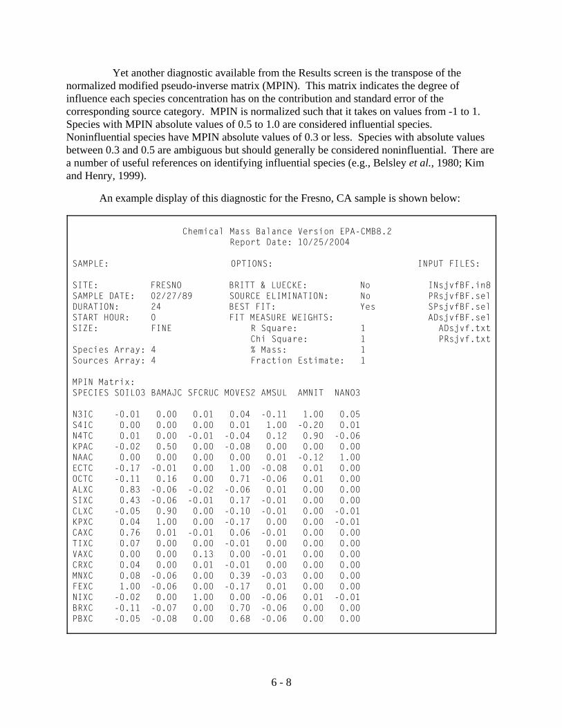
6 - 8

Chemical Mass Balance Version EPA-CMB8.2 Report Date: 10/25/2004 SAMPLE: OPTIONS: INPUT FILES: SITE: FRESNO BRITT & LUECKE: No INsjvfBF.in8SAMPLE DATE: 02/27/89 SOURCE ELIMINATION: No PRsjvfBF.selDURATION: 24 BEST FIT: Yes SPsjvfBF.selSTART HOUR: 0 FIT MEASURE WEIGHTS: ADsjvfBF.selSIZE: FINE R Square: 1 ADsjvf.txt Chi Square: 1 PRsjvf.txtSpecies Array: 4 % Mass: 1 Sources Array: 4 Fraction Estimate: 1 MPIN Matrix: SPECIES SOIL03 BAMAJC SFCRUC MOVES2 AMSUL AMNIT NANO3

N3IC -0.01 0.00 0.01 0.04 -0.11 1.00 0.05S4IC 0.00 0.00 0.00 0.01 1.00 -0.20 0.01N4TC 0.01 0.00 -0.01 -0.04 0.12 0.90 -0.06KPAC -0.02 0.50 0.00 -0.08 0.00 0.00 0.00NAAC 0.00 0.00 0.00 0.00 0.01 -0.12 1.00ECTC -0.17 -0.01 0.00 1.00 -0.08 0.01 0.00OCTC -0.11 0.16 0.00 0.71 -0.06 0.01 0.00ALXC 0.83 -0.06 -0.02 -0.06 0.01 0.00 0.00SIXC 0.43 -0.06 -0.01 0.17 -0.01 0.00 0.00CLXC -0.05 0.90 0.00 -0.10 -0.01 0.00 -0.01KPXC 0.04 1.00 0.00 -0.17 0.00 0.00 -0.01CAXC 0.76 0.01 -0.01 0.06 -0.01 0.00 0.00TIXC 0.07 0.00 0.00 -0.01 0.00 0.00 0.00VAXC 0.00 0.00 0.13 0.00 -0.01 0.00 0.00CRXC 0.04 0.00 0.01 -0.01 0.00 0.00 0.00MNXC 0.08 -0.06 0.00 0.39 -0.03 0.00 0.00FEXC 1.00 -0.06 0.00 -0.17 0.01 0.00 0.00NIXC -0.02 0.00 1.00 0.00 -0.06 0.01 -0.01BRXC -0.11 -0.07 0.00 0.70 -0.06 0.00 0.00PBXC -0.05 -0.08 0.00 0.68 -0.06 0.00 0.00

Yet another diagnostic available from the Results screen is the transpose of thenormalized modified pseudo-inverse matrix (MPIN). This matrix indicates the degree ofinfluence each species concentration has on the contribution and standard error of thecorresponding source category. MPIN is normalized such that it takes on values from -1 to 1. Species with MPIN absolute values of 0.5 to 1.0 are considered influential species. Noninfluential species have MPIN absolute values of 0.3 or less. Species with absolute valuesbetween 0.3 and 0.5 are ambiguous but should generally be considered noninfluential. There area number of useful references on identifying influential species (e.g., Belsley et al., 1980; Kimand Henry, 1999).

An example display of this diagnostic for the Fresno, CA sample is shown below:

6 - 9

( )FM

W W R W mass W FracEst

W W W W=

⎛⎝⎜

⎞⎠⎟ + + ⎛

⎝⎜⎞⎠⎟+

+ + +

1 2 22

3 4

1 2 3 4

1100χ

%

( )FM

W W R Wmass

W FracEst

W W W W=

⎛⎝⎜

⎞⎠⎟ + +

⎛⎝⎜

⎞⎠⎟ +

+ + +

1 2 22

3 4

1 2 3 4

1 100χ %

6.3 Best Fit Measure

As discussed in Section 3.2, when more that one species or sources selection arrays areprovided, EPA-CMB8.2 may be run in a Best Fit mode to have the model iterate among possiblecombinations of arrays and determine which results in an overall best fit. To do this, EPA-CMB8.2 uses a criterion called the Best Fit Measure that is calculated for each possible arraypair combination. The Best Fit Measure is a linear combination of four factors related tofundamental performance measures that are combined as follows:

% mass explained # 100

% mass explained > 100

Where

FM = Fit Measure

P2, R2, and % mass explained are the performance measures calculated by EPA-CMB8.2

FracEst is the ratio of the number of estimable fitting sources to the total number of fittingsources.

W1 = P2 weight

W2 = R2 weight

W3 = % mass weight

W4 = fraction estimated weight

As mentioned in Section 3.2, these weights are set to 1.0 by default, and may be changed in theOptions screen. And as mentioned in Section 5.1.3, for a given set of (non-negative) weightvalues, a larger value for FM corresponds to a better fit by EPA-CMB8.2.

7 - 1

7. REFERENCES

Anderson, E, Z. Bai, C. Bischof, S. Blackford, J. Demmel, J. Dongarra, J. Du Croz, A.Greenbaum, S. Hammarling, A. McKenney and D. Sorensen, 1999. LAPACK Users'Guide, Third Edition. Society for Industrial and Applied Mathematics (SIAM),Philadelphia, PA; ISBN 0-89871-447-8 (paperback).

Barth, D., 1970. Federal motor vehicle emissions goals for CO, HC, and NOx based ondesired air quality levels. JAPCA 20: 519.

Belsley, D.A., E. Kuh and R.E. Welsch, 1980. Regression Diagnostics: IdentifyingInfluential Data and Sources of Collinearity. John Wiley & Sons, Inc., New York.

Britt, H.I. and R.H. Luecke, 1973. The estimation of parameters in nonlinear, implicitmodels. Technometrics 15: 233.

Cass, G.R. and G.J. McRae, 1981. Minimizing the cost of air pollution control. Environ.Sci. Technol. 15: 748-57.

Chang, T.Y. and B. Weinstock, 1975. Generalized rollback modeling for urban air pollutioncontrol. JAPCA 25: 1033-7.

Cheng, M.D. and P.K. Hopke, 1989. Identification of markers for chemical mass balancereceptor model. Atmos. Environ. 23: 1373-84.

Chow, J.C., J.G. Watson, D.H. Lowenthal, L.C. Pritchett and L.W. Richards, 1990. SanJoaquin Valley Air Quality Study, Phase 2: PM10 modeling and analysis, Volume I:Receptor modeling source apportionment, Final Report. Report No. DRI 8929.1F,prepared by Desert Research Institute, Reno, NV.

Chow, J.C., J.G. Watson, D.H. Lowenthal, P.A. Solomon, K.L. Magliano, S.D. Ziman andL.W. Richards, 1992. PM10 source apportionment in California's San Joaquin Valley. Atmos. Environ. 26A: 3335-54.

Chow, J.C., J.G. Watson, D.M. Ono and C.V. Mathai, 1993. PM10 standards andnontraditional particulate source controls: A summary of the A&WMA/EPA internationalspecialty conference. JAWMA 43: 74-84.

Cooper, J.A. and J.G. Watson, 1980. Receptor oriented methods of air particulate sourceapportionment. JAPCA 30: 1116-25.

Coulter, C.T. and J.V. Scalco, 2005. Chemical Mass Balance Software: EPA-CMB8.2. Proceedings of A&WMA’s 98th Conference & Exhibition; Minneapolis, MN, June 21-24, 2005.

Currie, L.A., R.W. Gerlach, C.W. Lewis, W.D. Balfour, J.A. Cooper, S.L. Dattner, R.T.deCesar, G.E. Gordon, S.L. Heisler, P.K. Hopke, J.J. Shah, G.D. Thurston and H.J.Williamson, 1984. Interlaboratory comparison of source apportionment procedures:Results for simulated data sets. Atmos. Environ. 18: 1517.

deCesar, R.T., S.A. Edgerton, M.A.K. Khalil and R.A. Rasmussen, 1985. Sensitivityanalysis of mass balance receptor modeling: methyl chloride as an indicator of woodsmoke. Chemosphere 14: 1495-501.

7 - 2

deCesar, R.T., S.A. Edgerton, M.A.K. Khalil and R.A. Rasmussen, 1986. A tool fordesigning receptor model studies to apportion source impacts with specified precision. InTransactions, Receptor Methods for Source Apportionment: Real World Issues andApplications, Pace, T.G., editor. Air Pollution Control Association, Pittsburgh, PA. pp.56-67.

deNevers, N. and J.R. Morris, 1975. Rollback modeling: basic and modified. JAPCA 25:943.

Dzubay, T.G., R.K. Stevens, W.D. Balfour, H.J. Williamson, J.A. Cooper, J.E. Core, R.T.deCesar, E.R. Crutcher, S.L. Dattner, B.L. Davis, S.L. Heisler, J.J. Shah, P.K. Hopke andD.L. Johnson, 1984. Interlaboratory comparison of receptor model results for Houstonaerosol. Atmos. Environ. 18: 1555.

Environmental Protection Agency, 1990. Receptor Model Technical Series, Volume III(1989 Revision). CMB7 User's Manual. Report Number EPA-450/4-90-004. Office ofAir Quality Planning and Standards, Research Triangle Park, NC.

Environmental Protection Agency, 2004. Protocol for Applying and Validating the CMBModel for PM2.5 and VOC. Report No. EPA-451/R-04-001. December 2004. Office ofAir Quality Planning & Standards, Research Triangle Park, NC.

Friedlander, S.K., 1973. Chemical element balances and identification of air pollutionsources. Environ. Sci. Technol. 7: 235-40.

Friedlander, S.K., 1981. New developments in receptor modeling theory. In AtmosphericAerosol: Source/Air Quality Relationships, Macias, E.S. and Hopke, P.K., editors. American Chemical Society, Washington, D.C. pp. 1-19.

Fujita, E.M., J.G. Watson, J.C. Chow and Z. Lu, 1994. Validation of the chemical massbalance receptor model applied to hydrocarbon source apportionment in the SouthernCalifornia Air Quality Study. Environ. Sci. Technol. 28: 1633-49.

Gartrell, G. and S.K. Friedlander, 1975. Relating particulate pollution to sources: The 1972California Aerosol Characterization Study. Atmos. Environ. 9: 279-99.

Gordon, G.E., 1980. Receptor models. Environ. Sci. Technol. 14: 792-800.

Gordon, G.E., 1988. Receptor models. Environ. Sci. Technol. 22: 1132-1142.

Gordon, G.E., W.H. Zoller, G.S. Kowalczyk and S.W. Rheingrover, 1981. Composition ofsource components needed for aerosol receptor models. In Atmospheric Aerosol: Source/Air Quality Relationships, Macias, E.S. and Hopke, P.K., editors. American ChemicalSociety, Washington, D.C. pp. 51-74.

Henry, R.C., 1982. Stability analysis of receptor models that use least squares fitting. InReceptor Models Applied to Contemporary Air Pollution Problems, Hopke, P.K. andDattner, S.L., editors. Air Pollution Control Association, Pittsburgh, PA. pp. 141-62.

Henry, R.C., 1992. Dealing with near collinearity in chemical mass balance receptormodels. Atmos. Environ. 26A: 933-8.

7 - 3

Hidy, G.M. and S.K. Friedlander, 1972. The nature of the Los Angeles aerosol. In SecondInternational Clean Air Congress, Washington, D.C.

Hidy, G.M. and C. Venkataraman, 1996. The chemical mass balance method for estimatingatmospheric particle sources in Southern California. Chem. Eng. Comm. 151: 187-209.

Hopke, P.K., 1985. Receptor Modeling in Environmental Chemistry. John Wiley & Sons,New York, NY.

Hopke, P.K., 1991. Receptor Modeling for Air Quality Management. Elsevier Press,Amsterdam, The Netherlands.

Hopke, P.K. and S.L. Dattner, 1982. Receptor Models Applied to Contemporary PollutionProblems. Air & Waste Management Association, Pittsburgh, PA.

Hougland, E.S., 1983. Chemical element balance by linear programming. 73rd AnnualMeeting of the Air Pollution Control Association, Atlanta, GA.

Javitz, H.S. and J.G. Watson, 1986. Methods of receptor model evaluation and validation.In Transactions, Methods for Source Apportionment: Real World Issues andApplications, Pace, T.G, editor. Air Pollution Control Association, Pittsburgh, PA.

Javitz, H.S., J.G. Watson, J.P. Guertin and P.K. Mueller, 1988a. Results of a receptormodeling feasibility study. JAPCA 38: 661.

Javitz, H.S., J.G. Watson and N.F. Robinson, 1988b. Performance of the chemical massbalance model with simulated local-scale aerosols. Atmos. Environ. 22: 2309-22.

Kim, B.M. and R.C. Henry, 1989. Analysis of multicollinearity indicators and influentialspecies for chemical mass balance receptor model. In Transactions, Receptor Models inAir Resources Management, Watson, J.G., editor. Air & Waste ManagementAssociation, Pittsburgh, PA. pp. 379-90.

Kim, B.M. and R.C. Henry, 1999. Diagnostics for Determining Influential Species in theChemical Mass Balance Receptor Model. JAWMA 49: 1449-1455.

Kneip, T.J., M.T. Kleinman and M. Eisenbud, 1973. Relative contribution of emissionsources to the total airborne particulates in New York City. In Third International CleanAir Congress, Dusseldorf, FRG.

Larson, T.V. and R.J. Vong, 1989. Partial least squares regression methodology:Application to source receptor modeling. In Transactions, Receptor Models in AirResources Management, Watson, J.G., editor. Air & Waste Management Association,Pittsburgh, PA. pp. 391-403.

Lin, C. and J.B. Milford, 1994. Decay-adjusted chemical mass balance receptor modelingfor volatile organic compounds. Atmos. Environ. 28: 3261-76.

Lowenthal, D.H., R.C. Hanumara, K.A. Rahn and L.A. Currie, 1987. Effects of systematicerror, estimates and uncertainties in chemical mass balance apportionments: Quail RoostII revisited. Atmos. Environ. 21: 501-10.

7 - 4

Lowenthal, D.H. and K.A. Rahn, 1988a. Reproducibility of regional apportionments ofpollution aerosol in the Northeastern United States. Atmos. Environ. 22: 1829-33.

Lowenthal, D.H. and K.A. Rahn, 1988b. Tests of regional elemental tracers of pollutionaerosols. 2. Sensitivity of signatures and apportionments to variations in operatingparameters. Atmos. Environ. 22: 420-6.

Lowenthal, D.H., K.R. Wunschel and K.A. Rahn, 1988c. Tests of regional elemental tracersof pollution aerosols. 1. Distinctness of regional signatures, stability during transport, andempirical validation. Environ. Sci. Technol. 22: 413-20.

Lowenthal, D.H., J.C. Chow, J.G. Watson, G.R. Neuroth, R.B. Robbins, B.P. Shafritz andR.J. Countess, 1992. The effects of collinearity on the ability to determine aerosolcontributions from diesel- and gasoline-powered vehicles using the chemical massbalance model. Atmos. Environ. 26A: 2341-51.

Lowenthal, D.H., B. Zielinska, J.C. Chow, J.G. Watson, M. Gautam, D.H. Ferguson, G.R.Neuroth and K.D. Stevens, 1994. Characterization of heavy-duty diesel vehicleemissions. Atmos. Environ. 28: 731-44.

Miller, M.S., S.K. Friedlander and G.M. Hidy, 1972. A chemical element balance for thePasadena aerosol. J. Colloid Interface Sci. 39: 165-76.

Pace, T.G., 1986. Transactions, Receptor Methods for Source Apportionment: Real WorldIssues and Applications. Air Pollution Control Association, Pittsburgh, PA.

Pace, T.G., 1991. Receptor modeling in the context of ambient air quality standard forparticulate matter. In Receptor Modeling for Air Quality Management, Hopke, P.K.,editor. Elsevier, Amsterdam, The Netherlands. pp. 255-97.

Song, X.H. and P.K. Hopke, 1996. Solving the chemical mass balance problem using anartificial neural network. Environ. Sci. Technol. 30: 531

Stevens, R.K. and T.G. Pace, 1984. Review of the mathematical and empirical receptormodels workshop (Quail Roost II). Atmos. Environ. 18: 1499-506.

Venkataraman, C. and Friedlander, S.K., 1994. Source resolution of fine particulatepolycyclic aromatic hydrocarbons using a receptor model modified for reactivity. JAWMA 44: 1103-8.

Vong, R.J., P. Geladi, S. Wold and K. Esbensen, 1988. Source contributions to ambientaerosol calculated by discriminant partial least squares regression (PLS). J.Chemometrics 2: 281-96.

Watson, J.G., 1979. Chemical element balance receptor model methodology for assessingthe sources of fine and total particulate matter in Portland, Oregon. Ph.D. Dissertation. Oregon Graduate Center, Beaverton, OR.

Watson, J.G., 1984. Overview of receptor model principles. JAPCA 34: 619-23.

Watson, J.G. and J.C. Chow, 1994. Clear sky visibility as a challenge for society. AnnualRev. Energy Environ. 19: 241-66.

7 - 5

Watson, J.G., Cooper, J.A. and J.J. Huntzicker, 1984. The effective variance weighting forleast squares calculations applied to the mass balance receptor model. Atmos. Environ. 18: 1347-55.

Watson, J.G., J.C. Chow and C.V. Mathai, 1989. Receptor models in air resourcesmanagement: A summary of the APCA international specialty conference. JAPCA 39:419-26.

Watson, J.G., N.F. Robinson, J.C. Chow, R.C. Henry, B.M. Kim, T.G. Pace, E.L. Meyer andQ. Nguyen, 1990. The USEPA/DRI chemical mass balance receptor model, CMB 7.0. Environ. Software 5: 38-49.

Watson, J.G., J.C. Chow, Z. Lu, E.M. Fujita, D.H. Lowenthal and D.R. Lawson, 1994a. Chemical mass balance source apportionment of PM10 during the Southern California AirQuality Study. Aerosol Sci. Technol. 21: 1-36.

Watson, J.G., J.C. Chow, F.W. Lurmann and S. Misarra, 1994b. Ammonium nitrate, nitricacid, and ammonia equilibrium in wintertime Phoenix, Arizona. JAWMA 44: 405-12.

Williamson, H.J. and D.A. Dubose, 1983. Receptor model technical series, Volume III:User's manual for chemical mass balance model. Report No. EPA-450/4-83-014, U.S.Environmental Protection Agency, Research Triangle Park, NC.

Winchester, J.W. and G.D. Nifong, 1971. Water pollution in Lake Michigan by traceelements from aerosol fallout. Water Air and Soil Pollution 1: 50-64.

A - 1

APPENDIX A

THEORY OF THE CHEMICAL MASS BALANCE RECEPTOR MODEL

A - 2

A.1 INTRODUCTION

Receptor models use the chemical and physical characteristics of gases and particlesmeasured at source and receptor to both identify the presence of and to quantify sourcecontributions to the receptor. The particle characteristics must be such that: 1) they are presentin different proportions in different source emissions; 2) these proportions remain relativelyconstant for each source type; and 3) changes in these proportions between source and receptorare negligible or can be approximated.

Common types of receptor models include: (1) chemical mass balance (CMB); (2) principalcomponent analysis (PCA, otherwise known as factor analysis); and (3) multiple linearregression (MLR). Descriptions of these models and some of their variations are given in Henryet al. (1984) and Hopke (1991). Chemical mass balance is the fundamental receptor model, withall other approaches (including PCA and MLR) based on the use of the mass balance concept.

The chemical mass balance consists of a least squares solution to a set of linear equationswhich expresses each receptor concentration of a chemical species as a linear sum of products ofsource profile species and source contributions. The source profile species abundances (i.e., thefractional amount of the species in the emissions from each source-type) and the receptorconcentrations, with appropriate uncertainty estimates, serve as input data to the CMB model. The output consists of the amount contributed by each source-type to each chemical species. Themodel calculates values for the contributions from each source and the uncertainties of thosevalues. Input data uncertainties are used both to weight the importance of input data values inthe solution and to calculate the uncertainties of the source contributions.

A.2 CMB Mathematics

The source contribution (Sj) present at a receptor during a sampling period of length T dueto a source j with constant emission rate Ej is

(A-1)S D Ej j j= •

where:

(A-2)( ) ( )D d u t t x dtj j

T

= ⎡⎣⎢

⎤⎦⎥

→ →

∫ , ,σ0

is a dispersion factor depending on wind velocity (u), atmospheric stability (F), and the locationof source j with respect to the receptor (xj). All parameters in Equation A-2 vary with time, sothe instantaneous dispersion factor, Dj, must be integrated over time period T (Watson, 1979).

Various forms for Dj have been proposed (Pasquill, 1974; Benarie, 1976; Seinfeld andPandis, 1998), some including provisions for chemical reactions, removal, and specializedtopography. None are completely adequate to describe the complicated, random nature ofdispersion in the atmosphere. The advantage of receptor models is that an exact knowledge of Dj is unnecessary.

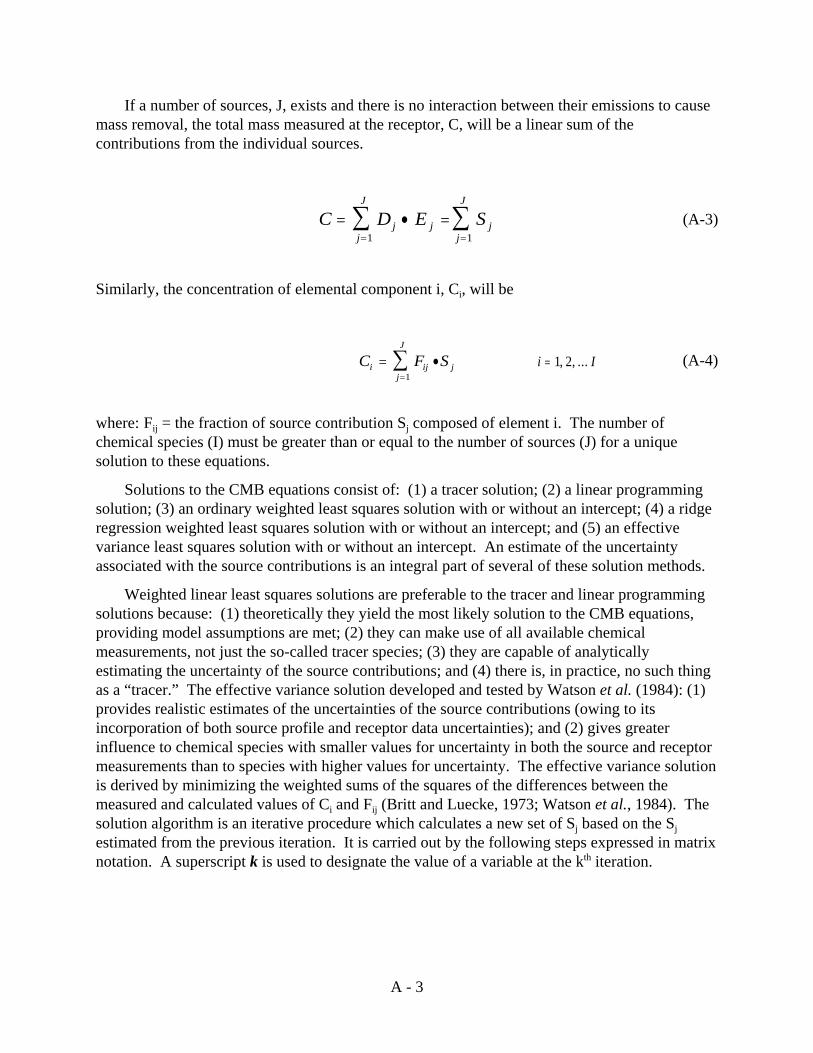
A - 3

If a number of sources, J, exists and there is no interaction between their emissions to causemass removal, the total mass measured at the receptor, C, will be a linear sum of thecontributions from the individual sources.

(A-3)C D E Sj jj

J

jj

J

= • == =∑ ∑

1 1

Similarly, the concentration of elemental component i, Ci, will be

(A-4)C F Si ijj

J

j= •=∑

1i I= 1 2, , ...

where: Fij = the fraction of source contribution Sj composed of element i. The number ofchemical species (I) must be greater than or equal to the number of sources (J) for a uniquesolution to these equations.

Solutions to the CMB equations consist of: (1) a tracer solution; (2) a linear programmingsolution; (3) an ordinary weighted least squares solution with or without an intercept; (4) a ridgeregression weighted least squares solution with or without an intercept; and (5) an effectivevariance least squares solution with or without an intercept. An estimate of the uncertaintyassociated with the source contributions is an integral part of several of these solution methods.

Weighted linear least squares solutions are preferable to the tracer and linear programmingsolutions because: (1) theoretically they yield the most likely solution to the CMB equations,providing model assumptions are met; (2) they can make use of all available chemicalmeasurements, not just the so-called tracer species; (3) they are capable of analyticallyestimating the uncertainty of the source contributions; and (4) there is, in practice, no such thingas a “tracer.” The effective variance solution developed and tested by Watson et al. (1984): (1)provides realistic estimates of the uncertainties of the source contributions (owing to itsincorporation of both source profile and receptor data uncertainties); and (2) gives greaterinfluence to chemical species with smaller values for uncertainty in both the source and receptormeasurements than to species with higher values for uncertainty. The effective variance solutionis derived by minimizing the weighted sums of the squares of the differences between themeasured and calculated values of Ci and Fij (Britt and Luecke, 1973; Watson et al., 1984). Thesolution algorithm is an iterative procedure which calculates a new set of Sj based on the Sjestimated from the previous iteration. It is carried out by the following steps expressed in matrixnotation. A superscript k is used to designate the value of a variable at the kth iteration.

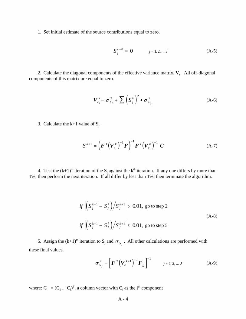
A - 4

1. Set initial estimate of the source contributions equal to zero.

(A-5)S jk = =0 0 j J= 1 2, , ...

2. Calculate the diagonal components of the effective variance matrix, Ve. All off-diagonalcomponents of this matrix are equal to zero.

(A-6)( )Vek

C jk

Fii i ijS= + •∑σ σ2

22

3. Calculate the k+1 value of Sj.

(A-7)( )( ) ( )S Ck Tek T

ek+ − − −

=1 1 1 1F V F F V

4. Test the (k+1)th iteration of the Sj against the kth iteration. If any one differs by more than1%, then perform the next iteration. If all differ by less than 1%, then terminate the algorithm.

go to step 2( )if S S Sjk

jk

jk+ +− >1 1 0 01. ,

go to step 5

(A-8)

( )if S S Sjk

jk

jk+ +− ≤1 1 0 01. ,

5. Assign the (k+1)th iteration to Sj and . All other calculations are performed withσ S j

these final values.

(A-9)( )[ ]σ ST

ek

jjj

2 1 1 1= + − −

F V F j J= 1 2, , ...

where: C = (C1 ... CI)T, a column vector with Ci as the ith component

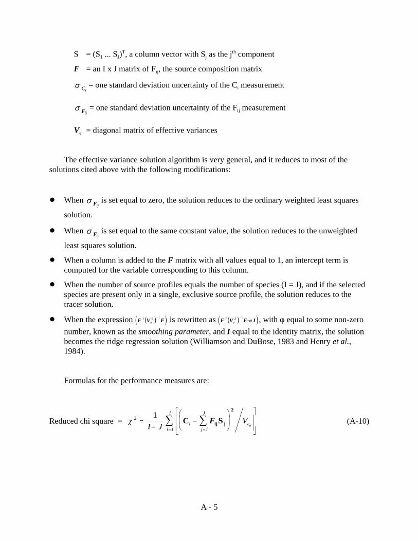
A - 5

S = (S1 ... SJ)T, a column vector with Sj as the jth component

F = an I x J matrix of Fij, the source composition matrix

= one standard deviation uncertainty of the Ci measurementσ Ci

= one standard deviation uncertainty of the Fij measurementσ Fij

Ve = diagonal matrix of effective variances

The effective variance solution algorithm is very general, and it reduces to most of thesolutions cited above with the following modifications:

! When is set equal to zero, the solution reduces to the ordinary weighted least squaresσ Fij

solution.

! When is set equal to the same constant value, the solution reduces to the unweightedσ Fij

least squares solution.

! When a column is added to the F matrix with all values equal to 1, an intercept term iscomputed for the variable corresponding to this column.

! When the number of source profiles equals the number of species (I = J), and if the selectedspecies are present only in a single, exclusive source profile, the solution reduces to thetracer solution.

! When the expression is rewritten as , with n equal to some non-zero( )( )F V FT ke

−1 ( )( )F V F- ITek −1

ϕ

number, known as the smoothing parameter, and I equal to the identity matrix, the solutionbecomes the ridge regression solution (Williamson and DuBose, 1983 and Henry et al.,1984).

Formulas for the performance measures are:

Reduced chi square = (A-10)χ 2 1=

−−

⎛

⎝⎜

⎞

⎠⎟

⎡

⎣⎢⎢

⎤

⎦⎥⎥==

∑∑I ij 1

J

i 1

I

JVeii

C Sij j

2

F

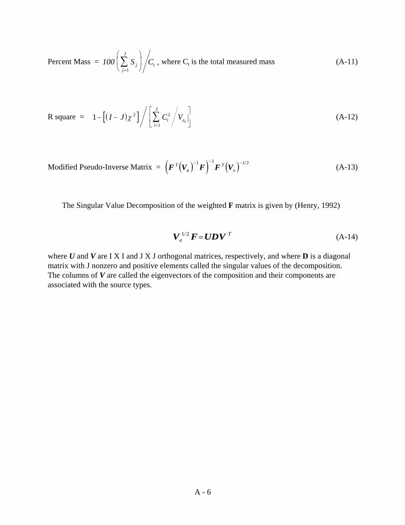
A - 6

Percent Mass = where Ct is the total measured mass (A-11)100 S Cjj

J

t=∑

⎛

⎝⎜

⎞

⎠⎟

1,

R square = (A-12)( )[ ]1 2 2

1− −

⎡

⎣⎢

⎤

⎦⎥

=∑I J C Vii

I

eiiχ

Modified Pseudo-Inverse Matrix = (A-13)( )( ) ( )F V F F VeT − − −1 1 1 2T

e

/

The Singular Value Decomposition of the weighted F matrix is given by (Henry, 1992)

(A-14)V F UDVeT1 2/ =

where U and V are I X I and J X J orthogonal matrices, respectively, and where D is a diagonalmatrix with J nonzero and positive elements called the singular values of the decomposition. The columns of V are called the eigenvectors of the composition and their components areassociated with the source types.

A - 7

References

Benarie, M.M., 1976. Urban Air Pollution Modeling Without Computers. U.S. EnvironmentalProtection Agency, Research Triangle Park, NC.

Britt, H.I. and R.H. Luecke, 1973. The estimation of parameters in nonlinear, implicit models. Technometrics 15, 233-233.

Henry, R.C., C.W. Lewis, P.K. Hopke, and H.J. Williamson, 1984. Review of receptor modelfundamentals. Atmos. Environ., 18, 1507-1515.

Henry, R.C., 1992. Dealing with near collinearity in chemical mass balance receptor models. Atmos. Environ. 26A, 933-938.

Hopke, P.K. (Ed.), 1991. Receptor Modeling for Air Quality Management. Elsevier SciencePublishing Company, Inc. New York, NY. 329pp.

Pasquill, F., 1974. Atmospheric Diffusion. Ellis Horwood, Chichester, England.

Seinfeld, J.H. and S.N. Pandis, 1998. Atmospheric Chemistry and Physics: From Air Pollutionto Climate Change. John Wiley & Sons, New York, NY.

Watson, J.G., 1979. Chemical Element Balance Receptor Model Methodology for Assessing theSources of Fine and Total Particulate Matter. Ph.D. Dissertation, Oregon Graduate Center,Beaverton, OR. University Microfilms International, Ann Arbor, MI.

Watson, J.G., Cooper, J.A., and J.J. Huntzicker, 1984. The effective variance weighting for leastsquares calculations applied to the mass balance receptor model. Atmos. Environ. 18, 1347-1355.

Williamson, H.J. and D.A. Dubose, 1983. Receptor model technical series, Volume III: User'smanual for chemical mass balance model. Report No. EPA-450/4-83-014, U.S.Environmental Protection Agency, Research Triangle Park, NC.

B - 1

APPENDIX B

Source Code for EPA-CMB8.2: Fortran & C++

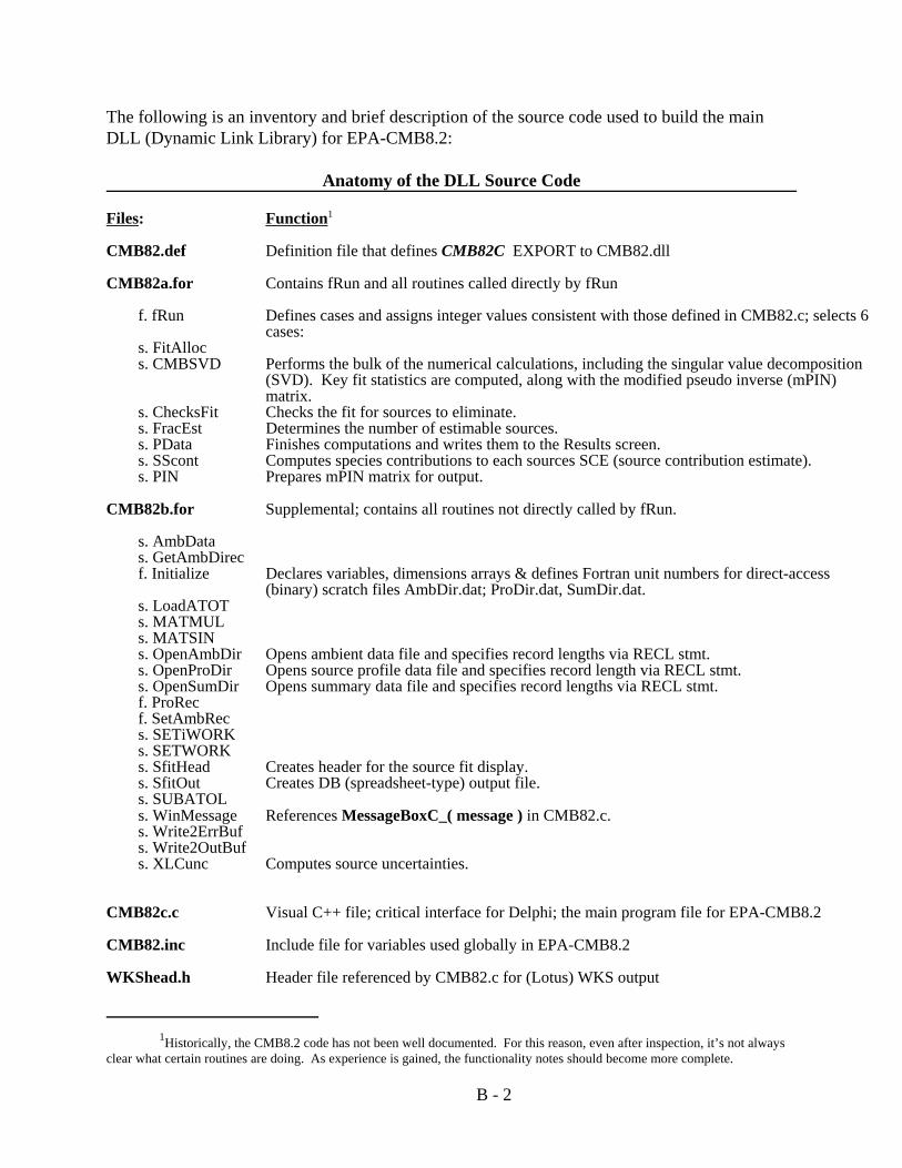
1Historically, the CMB8.2 code has not been well documented. For this reason, even after inspection, it’s not alwaysclear what certain routines are doing. As experience is gained, the functionality notes should become more complete.

B - 2

The following is an inventory and brief description of the source code used to build the mainDLL (Dynamic Link Library) for EPA-CMB8.2:

Anatomy of the DLL Source Code

Files: Function1

CMB82.def Definition file that defines CMB82C EXPORT to CMB82.dll

CMB82a.for Contains fRun and all routines called directly by fRun

f. fRun Defines cases and assigns integer values consistent with those defined in CMB82.c; selects 6cases:

s. FitAllocs. CMBSVD Performs the bulk of the numerical calculations, including the singular value decomposition

(SVD). Key fit statistics are computed, along with the modified pseudo inverse (mPIN)matrix.

s. ChecksFit Checks the fit for sources to eliminate.s. FracEst Determines the number of estimable sources.s. PData Finishes computations and writes them to the Results screen.s. SScont Computes species contributions to each sources SCE (source contribution estimate).s. PIN Prepares mPIN matrix for output.

CMB82b.for Supplemental; contains all routines not directly called by fRun.

s. AmbDatas. GetAmbDirecf. Initialize Declares variables, dimensions arrays & defines Fortran unit numbers for direct-access

(binary) scratch files AmbDir.dat; ProDir.dat, SumDir.dat.s. LoadATOTs. MATMULs. MATSINs. OpenAmbDir Opens ambient data file and specifies record lengths via RECL stmt.s. OpenProDir Opens source profile data file and specifies record length via RECL stmt.s. OpenSumDir Opens summary data file and specifies record lengths via RECL stmt.f. ProRecf. SetAmbRecs. SETiWORKs. SETWORKs. SfitHead Creates header for the source fit display.s. SfitOut Creates DB (spreadsheet-type) output file.s. SUBATOLs. WinMessage References MessageBoxC_( message ) in CMB82.c.s. Write2ErrBufs. Write2OutBufs. XLCunc Computes source uncertainties.

CMB82c.c Visual C++ file; critical interface for Delphi; the main program file for EPA-CMB8.2

CMB82.inc Include file for variables used globally in EPA-CMB8.2

WKShead.h Header file referenced by CMB82.c for (Lotus) WKS output

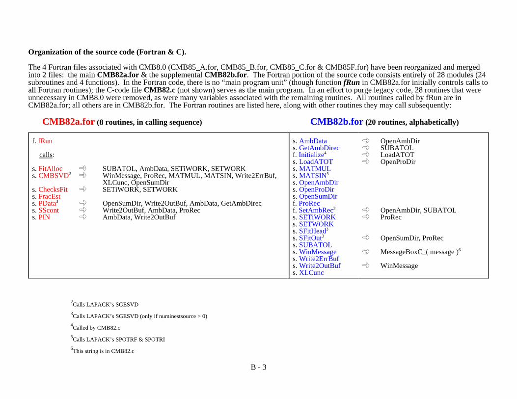
2Calls LAPACK’s SGESVD3Calls LAPACK’s SGESVD (only if numinestsource > 0)4Called by CMB82.c5Calls LAPACK’s SPOTRF & SPOTRI6This string is in CMB82.c

B - 3

Organization of the source code (Fortran & C).

The 4 Fortran files associated with CMB8.0 (CMB85_A.for, CMB85_B.for, CMB85_C.for & CMB85F.for) have been reorganized and mergedinto 2 files: the main CMB82a.for & the supplemental CMB82b.for. The Fortran portion of the source code consists entirely of 28 modules (24subroutines and 4 functions). In the Fortran code, there is no “main program unit” (though function fRun in CMB82a.for initially controls calls toall Fortran routines); the C-code file CMB82.c (not shown) serves as the main program. In an effort to purge legacy code, 28 routines that wereunnecessary in CMB8.0 were removed, as were many variables associated with the remaining routines. All routines called by fRun are inCMB82a.for; all others are in CMB82b.for. The Fortran routines are listed here, along with other routines they may call subsequently:

CMB82a.for (8 routines, in calling sequence) CMB82b.for (20 routines, alphabetically)

f. fRun

calls:

s. FitAlloc ¸ SUBATOL, AmbData, SETiWORK, SETWORKs. CMBSVD2 ± WinMessage, ProRec, MATMUL, MATSIN, Write2ErrBuf,

XLCunc, OpenSumDirs. ChecksFit ± SETiWORK, SETWORK s. FracEsts. PData3 ± OpenSumDir, Write2OutBuf, AmbData, GetAmbDirecs. SScont ± Write2OutBuf, AmbData, ProRecs. PIN ± AmbData, Write2OutBuf

s. AmbDatas. GetAmbDirecf. Initialize4

s. LoadATOTs. MATMULs. MATSIN5

s. OpenAmbDirs. OpenProDirs. OpenSumDirf. ProRecf. SetAmbRec3

s. SETiWORKs. SETWORKs. SFitHead3

s. SFitOut3

s. SUBATOLs. WinMessages. Write2ErrBufs. Write2OutBufs. XLCunc

± OpenAmbDir± SUBATOL± LoadATOT± OpenProDir

± OpenAmbDir, SUBATOL± ProRec

± OpenSumDir, ProRec

± MessageBoxC_( message )6

± WinMessage

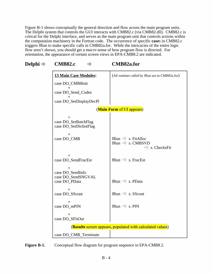
B - 4

Figure B-1 shows conceptually the general direction and flow across the main program units. The Delphi system that controls the GUI interacts with CMB82.c (via CMB82.dll). CMB82.c iscritical for the Delphi interface, and serves as the main program unit that controls actions withinthe computation machinery in the Fortran code. The occurrence of specific cases in CMB82.ctriggers fRun to make specific calls in CMB82a.for. While the intricacies of the entire logicflow aren’t shown, you should get a macro sense of how program flow is directed. Fororientation, the appearance of certain screen views in EPA-CMB8.2 are indicated.

Delphi ± CMB82.c ± CMB82a.for

13 Main Case Modules: (All routines called by fRun are in CMB82a.for)

case DO_CMB8init ?case DO_Send_Codes ?case DO_SetDisplayDecPl

( )

?case DO_SetBatchFlagcase DO_SetDichotFlag

?case DO_CMB fRun ± s. FitAlloc

fRun ± s. CMBSVD ¸ s. ChecksFit

?case DO_SendFracEst fRun ± s. FracEst

?case DO_SendInfocase DO_SendSNGVALcase DO_PData fRun ± s. PData

?case DO_SScont fRun ± s. SScont

?case DO_mPIN fRun ± s. PIN

?case DO_SFitOut

( )

case DO_CMB_Terminate

Figure B-1. Conceptual flow diagram for program sequence in EPA-CMB8.2.

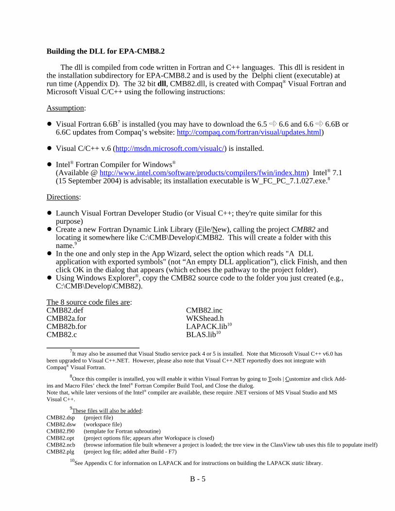
7It may also be assumed that Visual Studio service pack 4 or 5 is installed. Note that Microsoft Visual C++ v6.0 hasbeen upgraded to Visual C++.NET. However, please also note that Visual C++.NET reportedly does not integrate withCompaq® Visual Fortran.

8Once this compiler is installed, you will enable it within Visual Fortran by going to Tools | Customize and click Add-ins and Macro Files’ check the Intel® Fortran Compiler Build Tool, and Close the dialog.Note that, while later versions of the Intel® compiler are available, these require .NET versions of MS Visual Studio and MSVisual C++.

9These files will also be added:CMB82.dsp (project file)CMB82.dsw (workspace file)CMB82.f90 (template for Fortran subroutine)CMB82.opt (project options file; appears after Workspace is closed)CMB82.ncb (browse information file built whenever a project is loaded; the tree view in the ClassView tab uses this file to populate itself)CMB82.plg (project log file; added after Build - F7)

10See Appendix C for information on LAPACK and for instructions on building the LAPACK static library.

B - 5

Building the DLL for EPA-CMB8.2

The dll is compiled from code written in Fortran and C++ languages. This dll is resident inthe installation subdirectory for EPA-CMB8.2 and is used by the Delphi client (executable) atrun time (Appendix D). The 32 bit dll, CMB82.dll, is created with Compaq® Visual Fortran andMicrosoft Visual C/C++ using the following instructions:

Assumption:

! Visual Fortran 6.6B7 is installed (you may have to download the 6.5 ± 6.6 and 6.6 ± 6.6B or6.6C updates from Compaq’s website: http://compaq.com/fortran/visual/updates.html)

! Visual C/C++ v.6 (http://msdn.microsoft.com/visualc/) is installed.

! Intel® Fortran Compiler for Windows®

(Available @ http://www.intel.com/software/products/compilers/fwin/index.htm) Intel® 7.1(15 September 2004) is advisable; its installation executable is W_FC_PC_7.1.027.exe.8

Directions:

! Launch Visual Fortran Developer Studio (or Visual C++; they're quite similar for thispurpose)

! Create a new Fortran Dynamic Link Library (File/New), calling the project CMB82 andlocating it somewhere like C:\CMB\Develop\CMB82. This will create a folder with thisname.9

! In the one and only step in the App Wizard, select the option which reads "A DLL application with exported symbols" (not “An empty DLL application”), click Finish, and thenclick OK in the dialog that appears (which echoes the pathway to the project folder).

! Using Windows Explorer®, copy the CMB82 source code to the folder you just created (e.g.,C:\CMB\Develop\CMB82).

The 8 source code files are:CMB82.def CMB82.incCMB82a.for WKShead.hCMB82b.for LAPACK.lib10

CMB82.c BLAS.lib10

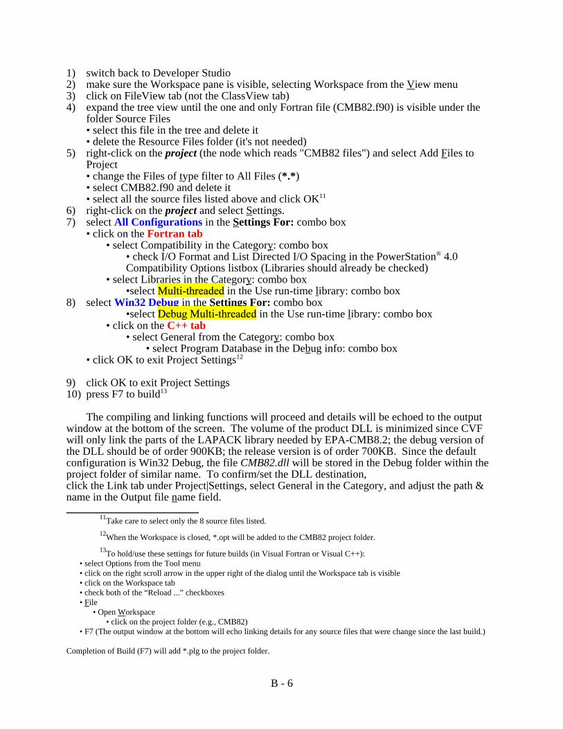
11Take care to select only the 8 source files listed.12When the Workspace is closed, *.opt will be added to the CMB82 project folder.13To hold/use these settings for future builds (in Visual Fortran or Visual C++):

• select Options from the Tool menu• click on the right scroll arrow in the upper right of the dialog until the Workspace tab is visible• click on the Workspace tab• check both of the “Reload ...” checkboxes• File

• Open Workspace• click on the project folder (e.g., CMB82)

• F7 (The output window at the bottom will echo linking details for any source files that were change since the last build.)

Completion of Build (F7) will add *.plg to the project folder.

B - 6

1) switch back to Developer Studio2) make sure the Workspace pane is visible, selecting Workspace from the View menu3) click on FileView tab (not the ClassView tab)4) expand the tree view until the one and only Fortran file (CMB82.f90) is visible under the

folder Source Files• select this file in the tree and delete it• delete the Resource Files folder (it's not needed)

5) right-click on the project (the node which reads "CMB82 files") and select Add Files toProject• change the Files of type filter to All Files (*.*)• select CMB82.f90 and delete it• select all the source files listed above and click OK11

6) right-click on the project and select Settings.7) select All Configurations in the Settings For: combo box

• click on the Fortran tab• select Compatibility in the Category: combo box

• check I/O Format and List Directed I/O Spacing in the PowerStation® 4.0Compatibility Options listbox (Libraries should already be checked)

• select Libraries in the Category: combo box•select in the Use run-time library: combo box

8) select Win32 Debug in the Settings For: combo box•select in the Use run-time library: combo box

• click on the C++ tab• select General from the Category: combo box

• select Program Database in the Debug info: combo box• click OK to exit Project Settings12

9) click OK to exit Project Settings10) press F7 to build13

The compiling and linking functions will proceed and details will be echoed to the outputwindow at the bottom of the screen. The volume of the product DLL is minimized since CVFwill only link the parts of the LAPACK library needed by EPA-CMB8.2; the debug version ofthe DLL should be of order 900KB; the release version is of order 700KB. Since the defaultconfiguration is Win32 Debug, the file CMB82.dll will be stored in the Debug folder within theproject folder of similar name. To confirm/set the DLL destination,click the Link tab under Project|Settings, select General in the Category, and adjust the path &name in the Output file name field.

C - 1

APPENDIX C

The Linear Algebra Library for EPA-CMB8.2: LAPACK

14Developed by Jack Dongarra, Jim Bunch, Cleve Moler and Pete Stewart; 1 Feb 1984. Available from NETLIB:http://www.netlib.org/linpack/

15The BLAS library includes the industry-standard Basic Linear Algebra Subprograms for Level 1 (vector-vector),Level 2 (matrix-vector), and Level 3 (matrix-matrix) applications.

C - 2

In order to solve the effective variance, least-squares regression that CMB employs for anapportionment, notably the Singular Value Decomposition (SVD), the Fortran code accesses alibrary of linear algebra routines. CMB8.0 relies on the linear algebra library LINPACK.14 LINPACK was designed for supercomputers in use in the 1970s and early 1980s and is acollection of Fortran subroutines that analyze and solve linear equations and linear least-squaresproblems. The package solves linear systems whose matrices are general, banded, symmetricindefinite, symmetric positive definite, triangular, and tridiagonal square. In addition, the packagecomputes the QR and SVDs of rectangular matrices and applies them to least-squares problems. LINPACK uses column-oriented algorithms to increase efficiency by preserving locality ofreference.

This library was up updated to LAPACK. LAPACK was developed by a consortium ofuniversity and government laboratories, and is the industry-standard subprogram package offeringan extensive set of linear system and eigenproblem solvers. Reference:

Anderson, E, Z. Bai, C. Bischof, S. Blackford, J. Demmel, J. Dongarra, J. Du Croz, A.Greenbaum, S. Hammarling, A. McKenney and D. Sorensen, 1999. LAPACK Users' Guide,Third Edition. Society for Industrial and Applied Mathematics (SIAM), Philadelphia, PA;ISBN 0-89871-447-8 (paperback) http://www.siam.org/

LAPACK is written in Fortran77 and provides routines for solving systems of simultaneouslinear equations, least-squares solutions of linear systems of equations, eigenvalue problems, andsingular value problems. The associated matrix factorizations (LU, Cholesky, QR, SVD, Schur,generalized Schur) are also provided, as are related computations such as reordering of the Schurfactorizations and estimating condition numbers. In all areas, similar functionality is provided forreal and complex matrices, in both single and double precision.

The original goal of the LAPACK project was to make the widely used LINPACK librariesrun efficiently on shared-memory vector and parallel processors. On these machines, LINPACKis inefficient because its memory access patterns disregard the multi-layered memory hierarchiesof the machines, thereby spending too much time moving data instead of doing useful floating-point operations. LAPACK addresses this problem by reorganizing the algorithms to use blockmatrix operations, such as matrix multiplication, in the innermost loops. These block operationscan be optimized for each architecture to account for the memory hierarchy (shared memory), andso provide a transportable way to achieve high efficiency on diverse modern machines. We usethe term "transportable" instead of "portable" because, for fastest possible performance, LAPACKrequires that highly optimized block matrix operations be already implemented on each machine.LAPACK routines are written so that as much as possible of the computation is performed by callsto the Basic Linear Algebra Subprograms (BLAS)15. While LINPACK is based on the vectoroperation kernels of the Level 1 BLAS, LAPACK was designed at the outset to exploit the Level 3BLAS - a set of specifications for Fortran subprograms that do various types of matrixmultiplication and the solution of triangular systems with multiple right-hand sides. Because ofthe coarse granularity of the Level 3 BLAS operations, their use promotes high efficiency onmany high-performance computers, particularly if specially coded implementations are provided

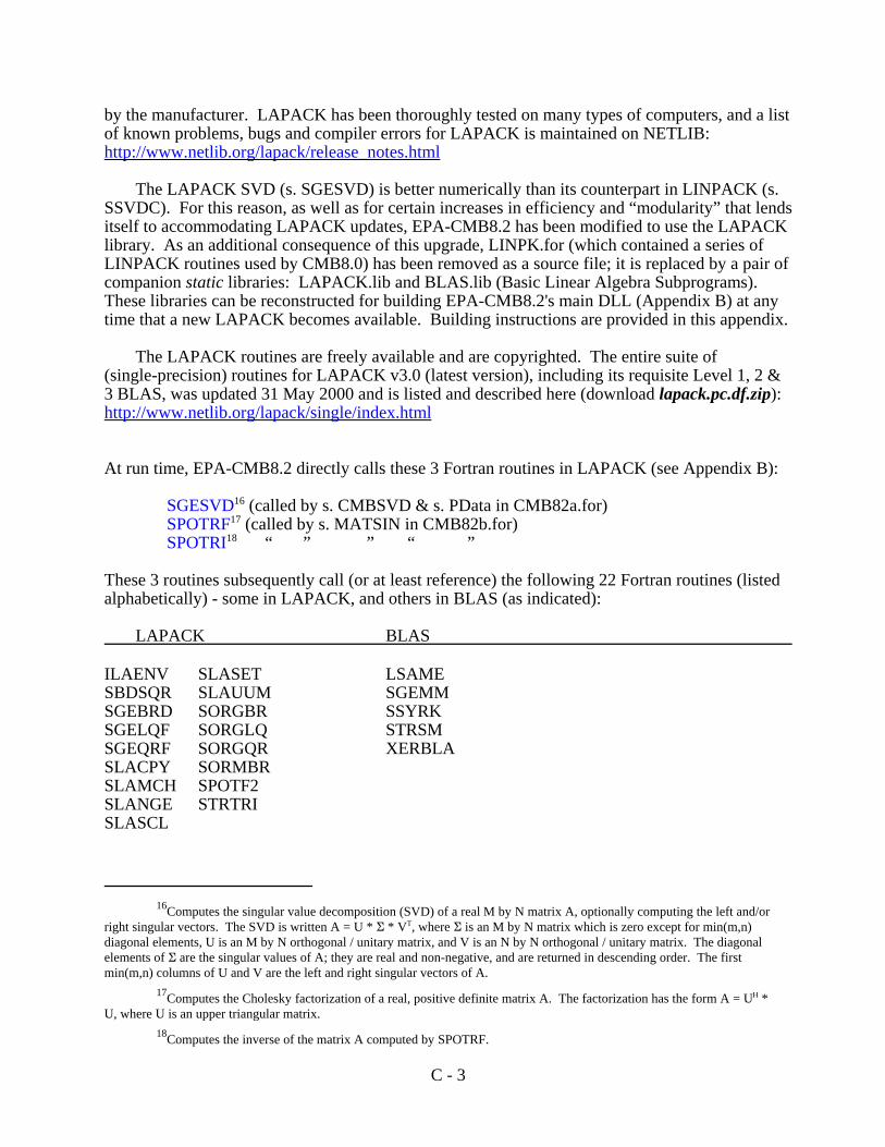
16Computes the singular value decomposition (SVD) of a real M by N matrix A, optionally computing the left and/orright singular vectors. The SVD is written A = U * E * VT, where E is an M by N matrix which is zero except for min(m,n)diagonal elements, U is an M by N orthogonal / unitary matrix, and V is an N by N orthogonal / unitary matrix. The diagonalelements of E are the singular values of A; they are real and non-negative, and are returned in descending order. The firstmin(m,n) columns of U and V are the left and right singular vectors of A.

17Computes the Cholesky factorization of a real, positive definite matrix A. The factorization has the form A = UH *U, where U is an upper triangular matrix.

18Computes the inverse of the matrix A computed by SPOTRF.

C - 3

by the manufacturer. LAPACK has been thoroughly tested on many types of computers, and a listof known problems, bugs and compiler errors for LAPACK is maintained on NETLIB:http://www.netlib.org/lapack/release_notes.html

The LAPACK SVD (s. SGESVD) is better numerically than its counterpart in LINPACK (s.SSVDC). For this reason, as well as for certain increases in efficiency and “modularity” that lendsitself to accommodating LAPACK updates, EPA-CMB8.2 has been modified to use the LAPACKlibrary. As an additional consequence of this upgrade, LINPK.for (which contained a series ofLINPACK routines used by CMB8.0) has been removed as a source file; it is replaced by a pair ofcompanion static libraries: LAPACK.lib and BLAS.lib (Basic Linear Algebra Subprograms). These libraries can be reconstructed for building EPA-CMB8.2's main DLL (Appendix B) at anytime that a new LAPACK becomes available. Building instructions are provided in this appendix.

The LAPACK routines are freely available and are copyrighted. The entire suite of(single-precision) routines for LAPACK v3.0 (latest version), including its requisite Level 1, 2 &3 BLAS, was updated 31 May 2000 and is listed and described here (download lapack.pc.df.zip):http://www.netlib.org/lapack/single/index.html

At run time, EPA-CMB8.2 directly calls these 3 Fortran routines in LAPACK (see Appendix B):

SGESVD16 (called by s. CMBSVD & s. PData in CMB82a.for)SPOTRF17 (called by s. MATSIN in CMB82b.for)SPOTRI18 “ ” ” “ ”

These 3 routines subsequently call (or at least reference) the following 22 Fortran routines (listedalphabetically) - some in LAPACK, and others in BLAS (as indicated):

LAPACK BLAS

ILAENV SLASET LSAMESBDSQR SLAUUM SGEMMSGEBRD SORGBR SSYRKSGELQF SORGLQ STRSMSGEQRF SORGQR XERBLASLACPY SORMBRSLAMCH SPOTF2SLANGE STRTRISLASCL

19It may also be assumed that Visual Studio service pack 4 or 5 is installed. Note that Microsoft Visual C++ v6.0 hasbeen upgraded to Visual C++.NET. However, please also note that Visual C++.NET reportedly does not integrate with CompaqVisual Fortran. You will likely have to use the Visual C++.NET environment separately to compile the C code, and then use thenewer linker to link the application.

20Eventually, all these files will also be added by CVF:LAPACK.dsp (project file)LAPACK.dsw (workspace file)LAPACK.ncb (browse information file built whenever a project is loaded; the tree view in the ClassView tab uses this file

to populate itself)LAPACK.plg (project log file)

21This will load the 1291 source files into the LAPACK project.

C - 4

Building the static LAPACK/BLAS Libraries for EPA-CMB8.2

To build the static LAPACK and companion BLAS libraries for EPA-CMB8.2 (see AppendixB), first obtain the 1291 LAPACK routines (12.2MB), and the 141 BLAS routines (966KB) fromthe source listed above.

Assumption:

! Visual Fortran 6.6B (or later)19 is installed (you may have to download the 6.5 ± 6.6 and 6.6± 6.6B or 6.6C updates from Compaq’s website:http://compaq.com/fortran/visual/updates.html)

! Intel® Fortran Compiler for Windows® (see footnote 8 in Appendix B)

Directions:

! Launch Visual Fortran Developer Studio (or Visual C++; they're quite similar for this purpose)! Create a new Fortran Static Library (File/New), calling the Workspace (and 1st project)

LAPACK and locating it somewhere like C:\CMB\Develop\CMB82. This will create a folderwith this name.20

Build the LAPACK library

1) Using Windows Explorer®, copy the LAPACK source code (*.f files) to the folder you justcreated (e.g., C:\CMB\Develop\LAPACK).

2) switch back to Developer Studio3) make sure the Workspace pane is visible, selecting Workspace from the View menu4) click on FileView tab (not the ClassView tab)5) expand the tree view delete the Header Files folder (it's not needed)6) right-click on the project (the node which reads "LAPACK files") and select Add Files to

Project• change the Files of type: filter to Fortran Files• select all the source files listed in the Look in: window and click OK21

22This will load the 141 source files into the BLAS project.23When the Workspace is closed, *.opt will be added to the LAPACK project folder.24Note that compilation of the 1291 LAPACK routines will take some time. Occasional informational messages of the

following type may be disregarded:Info: This directive is not supported in this platform.CDEC$ NOVECTOR---------------^

Completion of Build (F7) will add *.plg to the project folder.

C - 5

Build the companion BLAS library• right-click on the workspace (the node which reads Workspace ‘LAPACK':) and select AddNew Project to Workspace

• select Fortran Static Library, enter “BLAS” for Project name:, and click OK twice.• expand the tree view delete the Header Files folder (it's not needed)• Using Windows Explorer®, copy the BLAS source code (*.f files) to the folder you just

created (e.g., C:\CMB\Develop\CMB82\BLAS).• switch back to Developer Studio

• right click on the BLAS project and select Add Files to Project. Select the \BLASfolder and change the Files of type: filter to Fortran Files

• select all the source files listed in the Look in: window and click OK22

7) For both static library projects - LAPACK & BLAS - the Library Settings mustgenerally be set to match those for the main project (‘CMB82' - see Appendix B). Forboth LAPACK & BLAS:• right-click on the project and select Settings.• select All Configurations in the Settings For: combo box

• click on the Fortran tab• select Libraries in the Category: combo box

•select in the Use run-time library: combo box• click OK to exit Project Settings23

8) Build the libraries for both - LAPACK & BLAS - projects.• click Project\Set Active Project L LAPACK; press F7 to build24

• click Project\Set Active Project L BLAS; press F7 to build

As the compiling and linking functions will proceed for each build command, details will beechoed to the output window at the bottom of the screen. Since the default configuration is Win32Debug, the file(s) name.lib will be stored in the Debug folder within the respective project folderof similar name (this can be changed by clicking on the Library tab, then entering an alternatepath/file name in the Output file name: field).

D - 1

APPENDIX D

The User Interface for EPA-CMB8.2: Delphi

1Borland Software Corporation2The bulk of the application’s code is in MainFrm.pas and CMBInternals.pas. Delphi file types are described on p.

D - 3.

D - 2

The following lists and describes the source code, on which the Delphi1 client that serves as the User Interface (UI) for EPA-CMB8.2, is based:

Anatomy of the Delphi Source Code2

EPACMB82.res The project resource file. This is a binary file which normally contains theversion info resource (if required) and the application’s main icon. Changesto the version info and the application icon in Delphi’s Project Optionsdialog will result in changes to this file.

EPACMB82.dpr The Delphi project file. This is actually source code for the application: theproject file moniker is a misnomer.

EPACMB82.cfg The project configuration file. Stores the project configuration settings,primarily compiler and linker settings.

EPACMB82.dof The Delphi options file. Stores the project option settings, such asadditional compiler and linker settings, directories, conditional directives,and version information.

StartupFrm.pas / StartupFrm.frm The source code and form file for displaying thestartup screen, the first form shown when theapplication is run.

AboutFrm.pas / AboutFrm.dfm The source code and form file for displaying thebanner ‘About EPA-CMB8.2’.

BLWarningFrm.pas / BLWarningFrm.frm The source code and form file for displaying theBritt-Luecke warning message.

WaitFrm.pas / WaitFrm.dfm The source code and form file for displaying thetemporary ‘Please wait’ message, shown whenloading input data.

MainFrm.pas / MainFrm.dfm The source code and form file for displaying themain CMB model screen (Select Input Files;Options; Sample; Species; Sources; Results). About half of the application’s logic can befound in the source code for the main form.

D - 3

PrintOptionsFrm.pas / PrintOptionsFrm.dfm The source code and form file for displaying thePrint window enabled on the Results screenwhen the results are in the buffer. Most of thelogic for printing reports or saving them to a textfile can be found in the source code for the PrintOptions form.

SaveResultsFrm.pas / SaveResultsFrm.dfm The source code and form file for displaying theSave Results screen. This form allows saving ofthe current record or all included recordsdisplayed in the Main Report buffer. Most of thelogic for saving result data to a text file can befound in the source code for the Save Resultsform.

CMBInternals.pas Controls all Delphi setup and interaction withCMB82.c in calls to the C++/Fortran DLL. Alsocontains a number of math routines, e.g. Best Fit,and the code which refines the output reportgenerated by s. PData in CMB82a.for.

D - 4

General notes for Delphi file types:

*.pas Delphi source code file, called a unit (source code module), which is written in Pascal. Each application may contain several unit source files, which typically contain most ofthe code for the application.

*.dfm Delphi form file. A project-related file, *.dfm contains the description of the propertiesof the form and the components it owns. This description may be present in text form (aformat very suitable for version control) or in a compressed binary format. Each formfile represents a single form, which usually corresponds to a window or dialog box in anapplication. The Delphi IDE (Integrated Development Environment) allows you to viewand edit all form files as text, and to save form files as either text or binary. Eachapplication has at least one form and, while not all unit files (e.g., a math library offunctions and type information) have a corresponding form file, each form has acorresponding unit file (by default, having the same name as the form file). In the DelphiIDE, if a unit defines a form (i.e., uses a visual component such as TForm), a form file isautomatically created. N.B.: If a unit file (e.g., OptionsDlg.pas) defines a form andtherefore has a corresponding form file (e.g., OptionsDlg.dfm), both must be resident inthe working directory in order to open either in the IDE or Delphi will complain.

*.dpr Delphi project file. Another source file, *.dpr is explicitly created by association with aproject in the Delphi IDE. The project file (which corresponds to the ”main” programfile in traditional Pascal) organizes the unit files into an application. The Delphi IDEautomatically creates and maintains a unique project file for each application. Theproject file may be created by selecting a new project from the File menu in Delphi, e.g.,File | New Application. When the gallery dialog appears, double click on the iconentitled 'Application'. Delphi will then create a new project file for you. It will create afile called unit1.pas (and unit1.dfm) as a default because Delphi assumes that you want tohave a main form in your application.

*.dof Delphi options file. Contains the current settings for project options, such as compilerand linker settings, directories, conditional directives, command-line parameters andversion information. These are set using the Project Options dialog box (Project |Options), and Delphi saves them in text form for easy maintenance, version control, andsharing. Each project has an associated options file with the same name as the project(*.dpr) file.

*.res Delphi resource file. A project-related file, it contains the version information resource(if required) and the application's main icon. This file may also contain other resourcesused within the application but these are preserved as is. Do not delete this file if yourapplication contains any references to it.

*.cfg Project configuration file. This file stores project configuration settings and has the samename as the project file.

3N.B.: The original call in CMB8.0 to CMB8wn32.dll from:UNIT1.PAS(157): arg11, arg12 : Pointer ) : LongInt; stdcall; External 'cmb8wn32.dll' name '_CMB80C@52'

was changed in EPA-CMB8.2 to a call to CMB82.dll from: CMBInternals.pas(260): arg12: Pointer): Integer; stdcall; external 'CMB82.dll' name 'CMB82c'

D - 5

Construction of the Delphi executable for EPA-CMB8.2

The Delphi client (executable) calls CMB82.dll (Appendix B) at runtime. This client controls theuser interface for EPA-CMB8.2 and is created with Delphi 7, a product of Borland SoftwareCorporation (http://www.borland.com/delphi/), using the following instructions:.

Assumptions:

! Delphi 6 or 7 is installed.

Ordinarily, the compiler should be optimized for a build:Project | Options | Compiler | Code generation: check Optimization

Directions:

! Ensure that all of the following 19 Delphi source files are stored in a single working directory(folder):

EPACMB8.2.resEPACMB82.dprEPACMB82.cfgEPACMB8.2.dof

StartUpFrm.pas StartUpFrm.dfmAboutFrm.pas AboutFrm.dfmBLWarningFrm.pas BLWarningFrm.dfmWaitFrm.pas WaitFrm.dfmMainFrm.pas MainFrm.dfmPrintOptionsFrm.pas PrintOptions.Frm.dfmSaveResultsFrm.pas SaveResultsFrm.dfm

CMB82Internals.pas3

! Launch Delphi.! Select Open Project from the File menu.! Browse to the folder that contains the source files.! Select the file EPACMB82.dpr and click OK.! Select Build EPACMB82 from the Project menu.! The built executable should now appear in the working directory (folder), along with the

following compiled unit files (*.dcu):

D - 6

WaitFrm.dcuStartUpFrm.dcuSaveResultsFrm.dcuPrintOptions.Frm.dcuMainFrm.dcuBLWarningFrm.dcuAboutFrm.dcuCMBInternals.dcu

These intermediate *.dcu files , which are binary images for each unit file, are necessary to createthe final executable file (EPACMB82.exe). However, after the .exe has been created, you maydelete them. The next time you compile the application, the Delphi IDE will regenerate themautomatically.

E - 1

APPENDIX E

Warning and Error Messages from EPA-CMB8.2

1These messages originate from the Delphi client.

2If a model run does not converge, the results of that run will not be reliable. This does not have any negative impact on other successful runs within the same EPA-CMB8.2 session, so the other results may still be used.

E - 2

There are many different warning and error messages that EPA-CMB8.2 may produce to indicate that an input file is not namedproperly or does not follow the proper data format, that a model run is not set up correctly, or that a run did not produce satisfactoryresults. Most of the error messages that involve user intervention include suggestions for appropriate corrective actions. See AppendixF for a more detailed discussion of EPA-CMB8.2's behavior that may result in certain error conditions. A [] indicates a numeric valueor alphameric string.

CMBInternals.pas1

Error reading source selection filename. Please refer to the manual for file naming convention.Error reading species selection filename. Please refer to the manual for file naming convention.Error reading ambient data selection filename. Please refer to the manual for file naming convention.

Error reading ambient sample data filename. Please refer to the manual for file naming convention.The ambient sample data file does not exist.

Error reading source profiles data filename. Please refer to the manual for file naming convention.The source profiles data file does not exist.

**** NO CONVERGENCE AFTER [] ITERATIONS ****

AKT*VEFFIN*AK MATRIX NEEDS IMPROVEMENT. CHANGE FITTING SOURCES OR FITTING SPECIES.2

The number of fitting sources [] must be positive and <= the number of fitting species [].

Memory allocation error. Try shutting down other applications or increasing RAM.File Open Error. Check that the file exists or try rebooting.Species Set Error. Please see documentation regarding input file construction.Sources Set Error. Please see documentation regarding input file construction.The number of fitting sources must be positive and <= number of fitting species.

E - 3

Positive uncertainties are required for all fitting species and sources.This error should not occur. Contact Tom Coulter - [email protected] fitting source profiles matrix (Afit) contained a column of all zeros. Check the source profiles data file or change the fitting sources.The choices for fitting species and sources have produced a near-singular matrix. There is most likely collinearity between two or more of thefitting sources.The fitting algorithm failed to converge. There is most likely collinearity between two or more of the fitting sources.File Read Error. Please see documentation regarding input file construction.Unknown error.File Close Error. If your disk is full, try freeing up some space, or try rebooting.File Write Error. If your disk is full, try freeing up some space, or try rebooting.Ambient Data Error. Please see documentation regarding input file construction.Source Profiles Error. Please see documentation regarding input file construction.Error reading species selection file. Please see documentation regarding input file construction.Error reading source selection file. Please see documentation regarding input file construction.Error reading ambient data selection file. Please see documentation regarding input file construction.Error reading ambient data file. Please see documentation regarding input file construction.Error reading source profiles file. Please see documentation regarding input file construction.Memory free error. Try shutting down other applications or increasing RAM.

MainFrm.pas1

The ambient sample data file is empty!The ambient sample data file is open!Got an empty line of data from the ambient sample data file!The number of data values for this sample is wrong!Didn''t get any data from the ambient sample data file!The source profiles data file is empty!The source profiles data file is open!The source profiles selection file [] does not exist. Please edit the Control File and try again.The species selection file [] does not exist. Please edit the Control File and try again.The ambient data selection file [] does not exist. Please edit the Control File and try again.The ambient sample data file [] does not exist. Please edit the Control File and try again.The source profiles data file [] does not exist. Please edit the Control File and try again.Exactly *ONE* sample must be selected for the Best Fit option.The number of fitting species selected must be greater than or equal to the number of fitting sources selected.

3These messages originate from the C / Fortran DLL.

4The file listed may be either an ambient data (AD*.*) file or source profile (PR*.*) file; see Appendix F.

E - 4

The number of size ranges in the selected samples exceeds 4 for the same site and sampling period.

CMB82.c3

Can't open CMB8.2 ambient data file: [] (=> The file doesn’t exist, is open and locked (located?) elsewhere, or is read-only.)

Incorrect number of tokens in header line of file []. Should be an odd number > 5(=> The header line in the ambient sample data file is invalid.).

Total number of species = []

(Total #spp <= 0)Can't open CMB8.2 source profiles data file: []

(=> The file doesn’t exist, is open and locked (located?) elsewhere, or is read-only.)Can't create CMB8.2 direct access temporary file

(=> The file doesn’t exist, is open and locked (located?) elsewhere, is read-only, or the user’s machine is out of free disk space)Memory allocation error

(=> too many tokens)Number of tokens in line [] of file [] not equal to number of tokens in header line4

Total number of profiles data records = []

(Total #src profiles <=0)Memory allocation error for [] from line []Pointer [] not defined in ptinfo, line = []Unknown pointer [] from line []Memory overrun for pointer [] from line []; size = []Unknown action [] from line []Not able to open output file: []

5This error condition is caused by a column of the fitting matrix containing all zeros. The column corresponds to one of the fitting sources. A zero column for a fittingsource means that all of the fitting species' fractions are zero for that source. The fitting algorithm can't handle a zero column in the fitting matrix (it's the matrix equivalent ofdivision by zero).

6The AKT*VeffIn*AK matrix is used internally by the fitting algorithm. If one of its columns consists of elements close to zero, the algorithm has problems because ofcomputer round-off error, in which case MATSIN returns info = 1. This condition is usually caused by collinearity among fitting sources. Changing fitting sources and/or fittingspecies is intended to remove the collinearity.

E - 5

CMB82a.for2

(all in s.CMBSVD)

NUMBER OF FITTING SOURCES = [] > NUMBER OF FITTING SPECIES = []

FITTING SPECIES [] HAS ZERO AMBIENT DATA UNCERTAINTY.Replace uncertainty with a positive detection limit or remove the species from the fitting species list..

No record for source profile code [] and size []

Column (source) Number [] of Afit = 05

AKT*VeffIn*AK matrix needs improvement. Change fitting sources or fitting species.6

NO CONVERGENCE AFTER [] ITERATIONS.

F - 1

APPENDIX F

Data Input Issues for EPA-CMB8.2

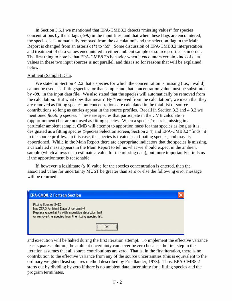
F - 2

In Section 3.6.1 we mentioned that EPA-CMB8.2 detects “missing values” for speciesconcentrations by their flags (-99.) in the input files, and that when these flags are encountered,the species is “automatically removed from the calculation” and the selection flag in the MainReport is changed from an asterisk (*) to ‘M’. Some discussion of EPA-CMB8.2 interpretationand treatment of data values encountered in either ambient sample or source profiles is in order. The first thing to note is that EPA-CMB8.2's behavior when it encounters certain kinds of datavalues in these two input sources is not parallel, and this is so for reasons that will be explainedbelow.

Ambient (Sample) Data.

We stated in Section 4.2.2 that a species for which the concentration is missing (i.e., invalid)cannot be used as a fitting species for that sample and that concentration value must be substitutedby -99. in the input data file. We also stated that the species will automatically be removed fromthe calculation. But what does that mean? By “removed from the calculation”, we mean that theyare removed as fitting species but concentrations are calculated in the total list of sourcecontributions so long as entries appear in the source profiles. Recall in Section 3.2 and 4.3.2 wementioned floating species. These are species that participate in the CMB calculation(apportionment) but are not used as fitting species. When a species’ mass is missing in aparticular ambient sample, CMB will attempt to apportion mass for that species as long as it isdesignated as a fitting species (Species Selection screen, Section 3.4) and EPA-CMB8.2 “finds” itin the source profiles. In this case, the species is treated as a floating species, and mass isapportioned. While in the Main Report there are appropriate indicators that the species is missing,a calculated mass appears in the Main Report to tell us what we should expect in the ambientsample (which allows us to estimate a value for the missing data), but more importantly it tells usif the apportionment is reasonable.

If, however, a legitimate ($ 0) value for the species concentration is entered, then theassociated value for uncertainty MUST be greater than zero or else the following error messagewill be returned :

and execution will be halted during the first iteration attempt. To implement the effective varianceleast squares solution, the ambient uncertainty can never be zero because the first step in theiteration assumes that all source contributions are zero. That is, in the first iteration, there is nocontribution to the effective variance from any of the source uncertainties (this is equivalent to theordinary weighted least squares method described by Friedlander, 1973). Thus, EPA-CMB8.2starts out by dividing by zero if there is no ambient data uncertainty for a fitting species and theprogram terminates.

F - 3

Source Profile Data.

For source profile input data files, we stated in Section 4.2.3 that missing mass fraction valuesmust be substituted by -99. and that the associated species will automatically be removed fromthe calculation. By this we mean that they are removed as fitting species and no concentrationsare calculated. If a mass fraction is substituted by -99. in the source profile data file, when EPA-CMB8.2 is run the value appearing for that species in the Main Report under “CALCULATED”will be a large negative value (if the value for number of decimal places displayed is set lowenough; Section 3.2). The values listed for the diagnostics CALCULATED/MEASURED andRESIDUAL/UNCERTAINTY will, of course, be meaningless. The value for the species inquestion listed in the Contribution by Species for the affected source will also be meaningless.

As we said in Section 4.2.3, while uncertainty values for species in source profiles areallowed to be # 0.0, some effort should be made to supply values > 0.0. However, for appropriatereasons, the same kinds of behavior (error messages, etc.) do not occur with equivalent input dataconditions as described above for the ambient data files. For example, if for a particular species ina source profile record the mass fraction is valid (i.e., $ 0.0), EPA-CMB8.2 allows an associateduncertainty value to be # 0.0. No error message will appear and EPA-CMB8.2 will executenormally.

Recall from Appendix A the effective variance weighting to which all of the ambientconcentrations are normalized. In Equation A-6, the effective variance is the concentrationuncertainty squared plus the sum of source contribution squared times the correspondingelemental mass fraction uncertainty squared:

Consider a situation for a woodsmoke profile in which the uncertainty for K (potassium) wasinput as # 0.0 for a mass fraction > 0.0.

If the uncertainty value for K < 0.0 (e.g., -99.), this uncertainty in the woodsmoke profile mayoverwhelm all of the other profile uncertainties (which are less than one because profiles arenormalized to unity). This would effectively remove K as a fitting species, because of division bythe effective variance resulting in a very low weight for this species. This will also propagate as avery high uncertainty on the source contribution estimate and on the calculated value for K.

If the uncertainty for K = 0.0, there are other components of the effective variance from the Kuncertainty in the ambient sample as well as from the K uncertainties in the other profiles, so thereis not division by zero just because K uncertainty in the woodsmoke profile is zero.

You may also obtain an unweighted least squares solution by setting all of the source profileuncertainties to zero and all of the ambient concentration uncertainties to the same value (e.g.,1.0). This gives the solution that you would get by multiple linear regression in a spreadsheet withthe intercept forced through zero. The solution in this case is dominated by the species with thehighest concentrations. Species such as Se (selenium) and V (vanadium) might get norepresentation with an unweighted least squares solution.

F - 4

For source profiles, in general, you wouldn’t enter a value of -99. for a species’ uncertaintyunless you also entered -99. for its abundance. A value of zero for a species’ uncertainty might beused for testing of least-squares approaches or for convenience, as illustrated in the exampleabove. In EPA-CMB8.2 the decision was explicitly made NOT to force (“hardwire”) sourceprofile uncertainties > 0.0 for the following reasons:

1. As noted above, zero uncertainties in the source profiles default to the ordinary weighted leastsquares (OWLS) method. This is a solution that some may still use. (Given what is known aboutthe dominance of source profile variability on the error, it has been shown that the OWLS solutionis biased compared with an effective variance solution.)

2. When data are unavailable for some components that are not likely to be in a source profile,you should insert zeros for the value and the uncertainty. An example is in the NFRAQS data set(Section 2.2), where we have lots of organic compounds for wood burning and cooking, and dieseland gasoline vehicles, but none for the soil or the road salt or the secondary ammonium nitrate andammonium sulfate. You could put in a zero entry and a very low uncertainty, e.g., 1x10-7, toindicate a detection limit. But this is essentially no different from zero when it is squared andadded into the effective variance with the uncertainties from those profiles that have real values. It is also effectively zero when compared to the ambient data uncertainty.

Source Profile Matrix: Afit

Sometimes a special situation may arise that affects the choice of fitting species (Section 3.4). This situation is likely to occur when single constituent sources are used as fitting sources. Singleconstituent sources are described elsewhere (e.g., EPA, 2004; Appendix G) but essentially involvethe designation of secondary compounds as “sources” to allow EPA-CMB8.2 to account forsecondarily formed materials observed in ambient samples. For such modeling scenarios,secondary compounds are involved that require selection of the constituent cations or anions. If, for example, you have sodium nitrate as a fitting source, but haven't selected (included) sodium ornitrate as fitting species, you will get a zero column in the source profiles (AFIT) matrix. Whenthis happens, the following error message can be returned when a calculation is attempted:

When ‘OK’ is clicked, the screen shown below appears. When EPA-CMB8.2 attempted toapportion the fitting sources to the ambient sample, it expected certain species for one or moresingle constituent sources (secondary compounds) that were excluded in the fitting species array.

This message will commonly appear when EPA-CMB8.2 is run in the Best Fit mode (Section3.2 & 5.2). As EPA-CMB8.2 advances through various corresponding pairs of fitting species andsource profile arrays, it is apt to encounter inappropriate combinations. The model will advancethrough all possible pairs, but will produce invalid results for the pairs that are ill-suited.

F - 5

Logic suggests that the 2nd line of the message should read: “... or change the fitting species.” Specifically for this example, the error message might have said (or been interpreted to say): "Select a fitting species that corresponds to a positive entry for that species in the NaNO3 profile." This error message will also be triggered for situations when there are many organic species and asoil profile when we eliminate all of the geological elements. We usually have zero entries for theorganics in the soil profile because we don't measure them. It also happens when a biogenic VOCsource profile is included but there's no isoprene, and for many of the single constituent solventand coating profiles (e.g., toluene, acetone, etc.).

Using EPA-CMB8.2 with Factors besides Chemical Abundance: e.g., Wind Direction.

As discussed above, an entry of -99. for species abundance (mass fraction) in a source profileautomatically removes that species from the source contribution calculation. It does not remove itfrom the concentration calculation if there is also an entry for that species in the ambient data file. This allowance of discrepancy, i.e., a valid (>0.0) value for a constituent in the ambient sampledata file and a value of -99. for its abundance in the source profile file(s), can be exploited forcases when we want to include other information in the ambient data file that is not appropriate forthe source profile. For example, wind direction (WD) can be included to indicate that an upwindsource profile should be used or not used. The -99. for this variable (factor) in the source profilefile does not allow it to be used as a fitting species, but the direction is still easily available for

F - 6

consultation when picking sources. This is more efficient (and convenient) than using a separatedata base or look-up table for WD. It also allows the source contributions to be stratified by winddirection (or other variable such as light scattering, temperature, or wind speed) by including it inthe ambient sample data (receptor) file.

The structure exists to display such external information corresponding to each sample that isnot, and cannot be, used as a fitting species. For example, one of the ways we recommend tochoose a profile for a sample is to determine if a source is upwind or downwind. For the sampleperiod(s) in question, the period-averaged WD can be imported directly into the ambient sampledata file as a “constituent” of each sample. The data file can thus be configured with a WDvariable into which you put the resultant wind direction, and set up a corresponding variable in thesource profile with a -99. value for “abundance”. This information can be easily viewed on-screen along with the species’ concentration information (Section 3.3). If, for example, you seethat the sample data indicate that it is downwind (± 5°) from a coal-fired power plant, and you alsosee a lot of selenium in this sample which doesn't appear in previous samples with prevailingwinds from opposite or very different directions, you may decide to include the power plantprofile, or retain a source combination you've already set up with that profile in it.

Highest wind speed during a sampling period is also good consideration for questions such as “Do I want the road dust or the windblown desert dust profile in this sample?” It's also usefulwhen you have other data, like CO and NOx, VOC, etc. at the receptor that might help you tochoose (and justify the choice of) a certain profile or source type, but which doesn't have an entryin any of your source profiles. By including these variables as sample “constituents”, it puts allthe information in front of you rather than forcing you to analyze from several different (external)sources of information.

ABSENT DATA

One condition in which EPA-CMB8.2’s behavior is parallel with respect to ambient sampleor source profile data is that of “absent data”. This condition is represented not by a flag for“missing” (invalid) data but rather the complete omission of the value from the input data record.

Ambient Sample Input File (AD*.*):

If a value for a species concentration, for example, is absent (omitted) from the ambientsample input data file, an error message such as the following will be returned:

as soon as EPA-CMB8.2 control is moved off of the Input Files screen. As indicated, on line 71of the ambient data input data file there is a missing (= absent) value. The following messageappears immediately after ‘OK’ is clicked on the message above:

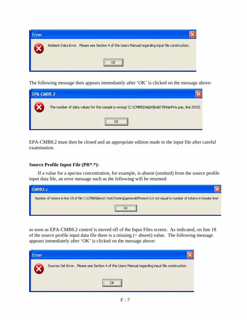
F - 7

The following message then appears immediately after ‘OK’ is clicked on the message above:

EPA-CMB8.2 must then be closed and an appropriate edition made to the input file after carefulexamination.

Source Profile Input File (PR*.*):

If a value for a species concentration, for example, is absent (omitted) from the source profileinput data file, an error message such as the following will be returned:

as soon as EPA-CMB8.2 control is moved off of the Input Files screen. As indicated, on line 18of the source profile input data file there is a missing (= absent) value. The following messageappears immediately after ‘OK’ is clicked on the message above:

F - 8

The following message then appears immediately after ‘OK’ is clicked on the message above:

As for the example illustrated above for the ambient data file, EPA-CMB8.2 must be closed andan appropriate edit be done on the input file.

G - 1

APPENDIX G

Notes on EPA-CMB8.2 Diagnostics

1This “combination” is important because a profile may be well separated for a high contribution, but it may fall withinthe uncertainties of the other profiles for a low contribution.

G - 2

EPA-CMB8.2's Main Report: EST

In the top portion of the Main Report is the diagnostic attribute “EST”, which may be either“YES” or “NO”. The manual states in several places (e.g., Sections 3.6.1 & 5.1.1) that “Thefield ‘EST’ under ‘SOURCE’ indicates (YES or NO) whether a source’s contribution wasestimable in EPA-CMB8.2's attempt at a fit, using the settings in Options.” This is also stated inTable 4.2-1 of the Protocol for Applying and Validating the CMB Model for PM-2.5 and VOC.(EPA, 2004). In particular, it is first order indication of whether or not the profile/sourcecontribution estimate combination1 meets or does not meet the criteria that have been set up inOptions. For any particular CMB fit, it is possible to set values for Maximum Source Uncertaintyand Minimum Source Projection in Options to indicate all YESs or all NOs (see below).

We currently don't know how those settings translate into useful information, as indicated bythe YESs and NOs. Unless you're researching how CMB responds to different combinations ofsource profiles and uncertainties, this parameter may not be very useful. The most importantevaluation parameter is the uncertainty of the source contribution estimate, which is a function ofthe input uncertainties and the collinearity (variance inflation). You'll notice that when you have anegative source contribution, it usually has a very high uncertainty and there is anothercompensating source contribution (usually a very high positive value) that also has a highuncertainty. This is a good indication that these are collinear. This is why the model gives theuncertainties and why they should be considered in decision-making, as described in the Protocolfor Applying and Validating the CMB Model for PM-2.5 and VOC. How to use this diagnostic ina practical setting has not been sufficiently studied. For now, it is really there for researchpurposes and not for everyday application.

In sensitivity testing for the two Options parameters mentioned above, the following has beenseen:

Maximum Source Uncertainty.

The default is value is 20%. As this value is reduced, the occurrence of NOs increases. Oncethis value is set to zero, EST = NO for all sources. Conversely, as this value is increased, theoccurrence of YESs will increase.

Minimum Source Projection.

The default value is 0.95%. As this value is substantially reduced, the occurrence of YESsincreases. As it approaches zero, EST = YES for all sources. If set to 1.00, EST = NO for allsources.

The array (pattern) of YES/NO under EST is fairly sensitive to settings of Maximum SourceUncertainty; it is fairly insensitive to settings for Minimum Source Projection. However,adjustment of these two parameters has an independent (and opposite) effect on the EST variable.

United States Office of Air Quality Planning and Standards Publication No. EPA-452/R-04-011

Environmental Protection Air Quality Strategies and Standards Division December 2004

Agency Research Triangle Park, NC

EPA-CMB8.2 User's Manual · EPA-CMB8.2 Users Manual By: C. Thomas Coulter ... several receptor...

Documents

Transcript of EPA-CMB8.2 User's Manual · EPA-CMB8.2 Users Manual By: C. Thomas Coulter ... several receptor...