Chemical Mass Balance Chemical Mass Balance Software: EPA-CMB8.2Software: EPA-CMB8.2

EPA-452/R-04-011 EPA-452/R-04-011 December 2004 December 2004

EPA-CMB8.2 Users ManualEPA-CMB8.2 Users Manual

Office of Air Quality Planning & StandardsOffice of Air Quality Planning & StandardsU.S. Environmental Protection AgencyU.S. Environmental Protection Agency

Research Triangle Park, NC 27711Research Triangle Park, NC 27711

Chemical Mass Balance Overview Chemical Mass Balance Overview

The CMB receptor model consists of a solution to linear equations that express each The CMB receptor model consists of a solution to linear equations that express each

receptor chemical concentration as a linear sum of products of source profile receptor chemical concentration as a linear sum of products of source profile

abundances and source contributions. abundances and source contributions.

For each run of CMB, the model fits speciated data from a specified group of sources For each run of CMB, the model fits speciated data from a specified group of sources

to corresponding data from a particular receptor sample. The source profile to corresponding data from a particular receptor sample. The source profile

abundances (i.e., the mass fraction of each source type) and the receptor abundances (i.e., the mass fraction of each source type) and the receptor

concentrations, with appropriate uncertainty estimates, serve as input data to CMB. concentrations, with appropriate uncertainty estimates, serve as input data to CMB.

The output consists of the amount contributed by each source type represented by a The output consists of the amount contributed by each source type represented by a

profile to the total mass, as well as to each chemical species. CMB calculates values profile to the total mass, as well as to each chemical species. CMB calculates values

for the contributions from each source and the uncertainties of those values. CMB is for the contributions from each source and the uncertainties of those values. CMB is

applicable to multi-species data sets, such as PM10, PM2.5, and VOCs. applicable to multi-species data sets, such as PM10, PM2.5, and VOCs.

References: Friedlander, 1973; Cooper and Watson, 1980; Gordon, 1980,References: Friedlander, 1973; Cooper and Watson, 1980; Gordon, 1980,1988 1988 ; Watson ; Watson

et al., 1984; 1990; 1991; Hidy and Venkataraman, 1996.et al., 1984; 1990; 1991; Hidy and Venkataraman, 1996.

Governing EquationGoverning Equation

• Ci is the ambient concentration of specie i;• aij is the fractional concentration of specie i in the

emissions from source j;• Sj is the total mass concentration contributed by

source j; and• p is the number of sources, and n is the number

of species, with n ≥ p.• The Ci and aij are known and the Sj are found by

a least squares solution of the over determined system of equations.

C a S i nij

p

ij j

1

1, ,

The CMB modeling procedure requires:The CMB modeling procedure requires:

1. identification of the contributing source types;

2. selection of chemical species or other properties to

be included in the calculation;

3. knowledge of the fraction of each of the chemical

species which is contained in each source

type )source profiles);

4. estimation of the uncertainty in both ambient

concentrations and source profiles; and

5. solution of the chemical mass balance equations.

Coarse Fraction - Neve ShaananDECEMBER 1995 - JA NUA RY 1996

V ar2

others , 0.1s oil r ic h Ca, 0.05s odium, 0.03

road dus t, 0.11

geologic al, 0.21

s ea s pray , 0.09

lime s tone, 0.41

Fine Fraction - Nev e ShaananDECEM BER 1995 - JANUARY 1996

Others , 35%

Sodium, 7%

Cement Kiln, 8%

Pow er plant, 9%

Dies el, 19%

Sea s pray , 2%A monium Sulf ate, 20%

CMB model assumptions are: CMB model assumptions are:

Compositions of source emissions are constant over the Compositions of source emissions are constant over the period period

of ambient and source sampling.of ambient and source sampling.

Chemical species do not react with each other.Chemical species do not react with each other.

All sources with a potential for contributing to the receptor have All sources with a potential for contributing to the receptor have

been identified and have had their emissions characterized.been identified and have had their emissions characterized.

The number of sources or source categories is less than or equal to The number of sources or source categories is less than or equal to

the number of species.the number of species.

The source profiles are linearly independent of each other. The source profiles are linearly independent of each other.

Measurement uncertainties are random, uncorrelated, and normally Measurement uncertainties are random, uncorrelated, and normally

distributed. distributed.

FEATURESFEATURES

• Windows®-based, • Multiple arrays for fitting species and

fitting sources• Britt-Luecke algorithm• Improved collinearity diagnostics• Better handling of VOC applications • Search for best fit • User-selected preferences

FEATURES (cont’d)FEATURES (cont’d)

• Negative source contributions• Improved memory management• Upgraded linear algebra library• Versatile graphic display capability• Context-sensitive on-line help• Flexible input and output formats• File handling

The EPA-CMB8.2 software website: www.epa.gov/scram001

EPA-CMB82.zip: the EPA-CMB8.2 executable, its companion DLL

file, and a help file.

EPA-CMB82 test.zip: all files needed for the test case (PM2.5 data,

ambient and source Profiles, from California’s San Joaquin Valley

Air Quality Study).

EPA-CMB82 Manual.pdf.

CMB Protocol.pdf: Protocol for Applying and Validating the CMB

Model for PM2.5 and VOC. This protocol is an important companion

document that provides useful guidance on interpreting CMB’s

diagnostic statistics and on assessing the integrity of its

apportionments.

Source82.zip: A compressed file of EPA-CMB8.2 source code (EPA-

CMB8.2 software is written in the Fortran, C++, and Delphi (Pascal)

computer languages).

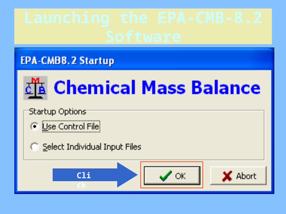
Launching the EPA-CMB-8.2 Software

Click

Browse Dialog forSelecting a Control File

Click

We load the San Joaquin Valley Fine data set (Chow et al., 1992).

Cli

ck

Banner Page

via

Help | About

Click

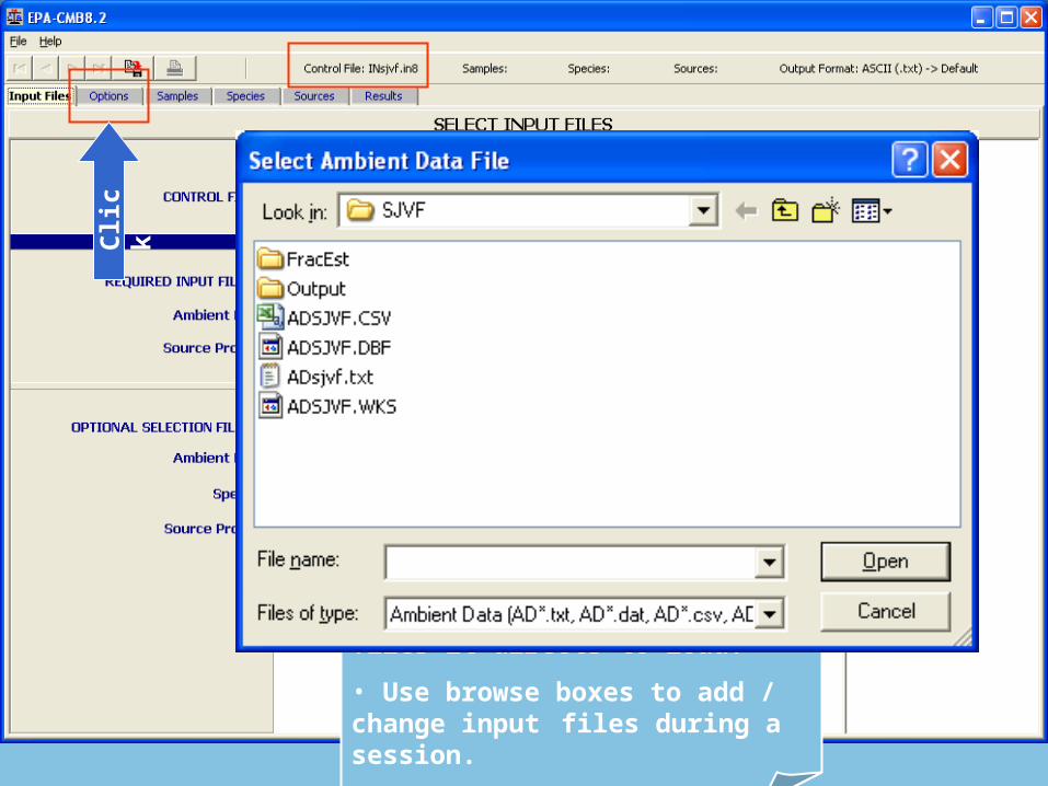
• Control File name is echoed, as are any input files it directs to load.

• Use browse boxes to add / change input files during a session.

Cli

ck

Click

This parameter sets the maximum number of iterations EPA-CMB8.2 will attempt to arrive at a solution. If no convergence can be achieved, there is probably excessive collinearity for this sample and combination of fitting sources. Its value is adjusted via the spinners. (Must be >0; no theoretical upper limit; default = 20)

Allows the eligible space collinearity evaluation method of Henry (1992) to be implemented with each CMB calculation. The maximum source uncertainty is a threshold expressed as a percentage of the total measured mass and is adjustable via the spinners (default = 20% ; acceptable range 0 - 100).

Allows the eligible space collinearity evaluation method of Henry (1992) to be implemented with each CMB calculation. The minimum source projection is set to a default value of 0.95 (acceptable range 0.0 - 1.0), but can be changed in the display field.

This parameter sets the number of decimal places displayed in the output window and output files. Depends on the units used in the input data files. Setting affects the display columns for source contributions estimates, measured species concentrations (ambient samples and source profiles), calculated contributions by species, as well as for inverse singular values. Adjusted by using the spinners. The default value is 5 and the maximum value is 6.

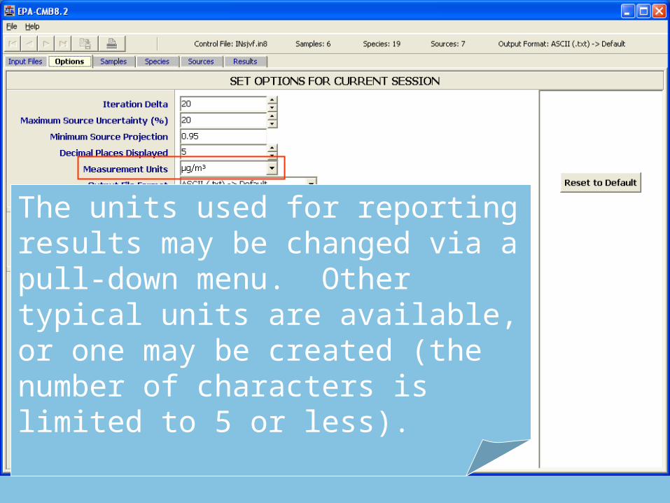
The units used for reporting results may be changed via a pull-down menu. Other typical units are available, or one may be created (the number of characters is limited to 5 or less).

File format for spreadsheet-type output is selected in the pull-down box. Default is ASCII (txt); comma-separated value (CSV) is also available. Selection is echoed on the status bar at the top of the screen.

Checking this box applies the Britt and Luecke (1973) linear least squares solution explained by Watson et al. (1984) when applied to CMB calculations. Allows the source profiles used in the fit calculation to vary, and enables a general solution to the least squares estimation that includes uncertainty in all the variables (i.e., the source compositions as well as the ambient concentrations).

Checking this box eliminates negative source contributions from the calculation, one at a time. After each fit attempt, if any sources have negative contributions, the source with the largest negative contribution is eliminated and another fit is attempted. Process is repeated until EPA-CMB8.2 finds no sources with negative contributions. Invocation of this option affects the fit obtained by effectively removing collinear sources.

Causes the program to cycle through the corresponding pairs (same array index) of fitting species and source profile arrays specified in the source and species selection input windows until best composite Fit Measure has been achieved. The fit with the largest Fit Measure is then displayed and becomes the current fit. After a Best Fit has been made, the fitting species and fitting sources arrays will be tagged (highlighted) in their respective windows.

Weights (coefficients) applied to each of the performance measures chi square, r-square, percent mass, and fraction of eligible sources. Positive values between 0 and 1 may be entered by typing into the appropriate display fields. Defaults are 1.0 for each performance measure weight.

Cli

ck

Click

Click

Collapsed list of samples.

Cli

ck

Cli

ck

Click Index Number

Cli

ck

Click Index Number

Cli

ck

Cli

ck

Cli

ck

Cli

ck

Collapsed view for Array 5

NB: Sample selection will be retained following the batch calculation. Samples can easily be DEselected and REselected on the Ambient Data Samples screen.

Cli

ck

Cli

ck

Batch run for the 6 samples tagged …

3rd result of the 6 in the buffer …

SUM

Cli

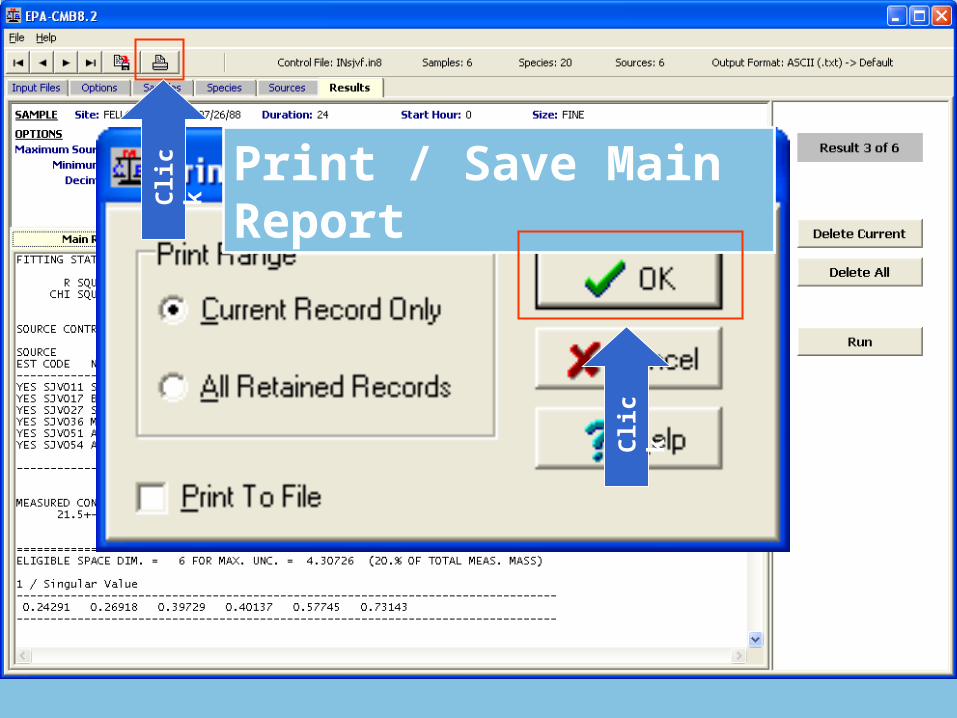
ck Print / Save Main Report

Cli

ck

Cli

ck

Click

Cli

ck

Cli

ck

Save spreadsheet-type results

Click

SPcode SPname I SiteID DATE ST DR SIZE Mconc Munc Cconc Cunc Rsquare CHIsqr %MASS SJV001 SOIL01TMAC TMAU FELLOW 07/26/88 0 24 FINE 21.53630 1.19000 20.61957 1.05551 0.91276 4.86863 95.74332 4.72533 0.30812N3IC N3IU * FELLOW 07/26/88 0 24 FINE 0.21280 0.18520 0.25688 0.05922 0.91276 4.86863 95.74332 0.01276 0.02221S4IC S4IU * FELLOW 07/26/88 0 24 FINE 5.14750 0.27090 5.64551 0.50730 0.91276 4.86863 95.74332 0.00189 0.00614N4TC N4TU * FELLOW 07/26/88 0 24 FINE 1.91540 0.13330 1.72104 0.17520 0.91276 4.86863 95.74332 0.00284 0.00236KPAC KPAU * FELLOW 07/26/88 0 24 FINE 0.11510 0.02380 0.10179 0.03801 0.91276 4.86863 95.74332 0.00473 0.00142NAAC NAAU * FELLOW 07/26/88 0 24 FINE 0.14880 0.05830 0.13499 0.03160 0.91276 4.86863 95.74332 0.00425 0.00189ECTC ECTU * FELLOW 07/26/88 0 24 FINE 0.81720 0.19810 1.81263 0.49971 0.91276 4.86863 95.74332 0.12995 0.05434OCTC OCTU * FELLOW 07/26/88 0 24 FINE 3.89260 0.45780 2.74572 0.61583 0.91276 4.86863 95.74332 0.48482 0.06521ALXC ALXU * FELLOW 07/26/88 0 24 FINE 0.29510 0.03000 0.44982 0.05106 0.91276 4.86863 95.74332 0.44796 0.05103SIXC SIXU * FELLOW 07/26/88 0 24 FINE 0.94330 0.06120 1.17369 0.13467 0.91276 4.86863 95.74332 1.15014 0.13042SUXC SUXU _ FELLOW 07/26/88 0 24 FINE 2.01640 0.10200 1.83451 0.15798 0.91276 4.86863 95.74332 0.00945 0.00520CLXC CLXU * FELLOW 07/26/88 0 24 FINE 0.02750 0.00710 0.05008 0.01515 0.91276 4.86863 95.74332 0.00331 0.00047KPXC KPXU * FELLOW 07/26/88 0 24 FINE 0.16320 0.01060 0.14503 0.02987 0.91276 4.86863 95.74332 0.04867 0.00567CAXC CAXU * FELLOW 07/26/88 0 24 FINE 0.17820 0.01160 0.09446 0.01020 0.91276 4.86863 95.74332 0.08836 0.00992TIXC TIXU * FELLOW 07/26/88 0 24 FINE 0.02980 0.00690 0.02505 0.00288 0.91276 4.86863 95.74332 0.02457 0.00284VAXC VAXU * FELLOW 07/26/88 0 24 FINE 0.03660 0.00370 0.03836 0.00275 0.91276 4.86863 95.74332 0.00142 0.00047CRXC CRXU * FELLOW 07/26/88 0 24 FINE 0.00660 0.00180 0.00187 0.00090 0.91276 4.86863 95.74332 0.00142 0.00000MNXC MNXU * FELLOW 07/26/88 0 24 FINE 0.00580 0.00100 0.00632 0.00075 0.91276 4.86863 95.74332 0.00520 0.00047FEXC FEXU * FELLOW 07/26/88 0 24 FINE 0.27460 0.01830 0.28496 0.03120 0.91276 4.86863 95.74332 0.27549 0.03119NIXC NIXU * FELLOW 07/26/88 0 24 FINE 0.03790 0.00230 0.03604 0.00405 0.91276 4.86863 95.74332 0.00047 0.00000CUXC CUXU _ FELLOW 07/26/88 0 24 FINE 0.13830 0.06990 0.00059 0.00007 0.91276 4.86863 95.74332 0.00047 0.00000ZNXC ZNXU _ FELLOW 07/26/88 0 24 FINE 0.09320 0.04160 0.01606 0.00178 0.91276 4.86863 95.74332 0.00095 0.00000BRXC BRXU _ FELLOW 07/26/88 0 24 FINE 0.01080 0.00080 0.00708 0.00367 0.91276 4.86863 95.74332 0.00047 0.00000PBXC PBXU * FELLOW 07/26/88 0 24 FINE 0.02310 0.00540 0.00900 0.00500 0.91276 4.86863 95.74332 0.00000 0.00000

Left-hand side of the spreadsheet-type output file …

Cli

ck

Cli

ck

Modified Pseudo-Inverse Normalized Matrix