Earth Planets Space, 57, 605–612, 2005

Electrical conductivity structures estimated by thin sheet inversion, withspecial attention to the Beppu-Shimabara graben in central Kyushu, Japan

Shun Handa

Faculty of Agricultural Science, Saga University, Honjo 1, Saga 840-8502, Japan

(Received February 3, 2005; Revised April 25, 2005; Accepted May 11, 2005)

It is proposed that the Beppu-Shimabara graben (BSG), characterized by the continuous negative Bougueranomaly, runs NE to SW in central Kyushu. In order to clarify the BSG, the shallow electrical conductivitystructure in central Kyushu is obtained by thin sheet modeling using the inversion of a conjugate gradientrelaxation method and also using the forward method. The data used are the single-site transfer functions at75 sites for the periods of 77, 97 and 122 sec. The inverted model indicates three highly conductive areas: theseare the Saga-Chikugo plain covered with thick alluvium and the eastern and the western parts of central Kyushuincluding the BSG. Both end zones of this BSG are highly conductive in our model, which is closely related toconductive layers shallower than about 1 km. In contrast, the central part of the BSG is rather highly resistive.The BSG, thus, is not revealed as a continuous high-conductive belt and seems to be separated into three parts;the eastern and the western high-conductive zones and the central resistive area in our geoelectrical model of theshallow crust.Key words: Electrical conductivity, Beppu-Shimabara graben, thin sheet model, inversion, GDS.

1. IntroductionCentral Kyushu is a tectonically active region; four

volcanoes—Tsurumi, Kuju, Aso, and Unzen (Fig. 1)—areactive now and earthquakes occur frequently in the shal-low crust. In this region, the NS extensional strain fieldis dominant, in contrast to the EW compressional field inother areas of Japan. As a result, the active fault systemsof a normal fault-type are well developed, especially in theBeppu area and the Shimabara Peninsula where the grabensare formed. Matsumoto (1979) pointed out that eruptedvolcanic rocks covering wide areas are closely related tothe formation of these basinal features. He then proposedthe Beppu-Shimabara graben (BSG) running through cen-tral Kyushu in a NE-SW direction as shown in Fig. 1. Ana-lyzing the focal mechanism of shallow earthquakes, Eguchiand Uyeda (1983) suggested that this graben is a rift zonein the northeastern extension of the Okinawa Trough.

Some geological and petrologic results, however, do notseem to support a close relationship between the BSG andthe formation of volcanoes. In central-eastern Kyushu,eruptions ejecting a large quantity of volcanic rocks tookplace between 6 and 1 Ma in a triangular region surroundedby the tectonic lines of Matsuyama-Imari (MIL) and Oita-Kumamoto (OKL) and the southern extension (HHL) of theKokura-Tagawa fault zone (Kamata, 1989). Kamata (1989)pointed out that this area, which he called the Hohi volcaniczone, is a volcano-tectonic depression where the formationof the zone and eruptions occur simultaneously, and thusthe rifting of the Okinawa Trough hardly supports this con-

Copy right c© The Society of Geomagnetism and Earth, Planetary and Space Sci-ences (SGEPSS); The Seismological Society of Japan; The Volcanological Societyof Japan; The Geodetic Society of Japan; The Japanese Society for Planetary Sci-ences; TERRAPUB.

jecture. Moreover, Unzen Volcano in the Shimabara grabenis a different type of volcano from the other three activevolcanoes in volcanological and structural history (Kamata,1989) as well as in the chemical composition of its magmasource (Nakada and Kamata, 1991).

Although the BSG is one of the most important themesin the tectonics of Kyushu, as mentioned above, the struc-ture is not well understood, because central Kyushu iscommonly covered with volcanic formations and basementrocks appear only in narrow areas, as shown in Fig. 1. Inorder to investigate the electrical structures beneath centralKyushu, we have conducted geomagnetic depth sounding(GDS) studies since 1983 (Handa et al., 1992). The elec-trical conductivity models (Handa et al., 1992; Shimoizumiet al., 1997) based on these data, indicate the following re-sults: the in-phase induction arrows, i.e., Parkinson’s ar-rows (Parkinson, 1962), for periods of longer than 5 mintend to point towards the west or the southwest in centralKyushu. This direction is partly explained by the land-seaconfiguration, but to fully account for it, there must be ahigh-conductive layer in the upper mantle under the EastChina Sea.

In the previous study (Handa et al., 1992), modeling wasperformed by focusing on the deep structure of the lowercrust and the upper mantle, as the observation sites usedwere insufficient to discuss the detailed structure of theshallow crust. Since 1989, we have conducted new GDSobservations at 55 sites. These GDS data at the sites thatare densely and widely distributed permit the constructionof the electrical conductivity model in the entire region ofthe BSG. Thus, by using the thin sheet modeling technique,we will discuss the shallow resistivity structure, mainlyof the BSG in central Kyushu, which is expected to be

605

606 S. HANDA: ELECTRICAL CONDUCTIVITY STRUCTURES ESTIMATED BY THIN SHEET INVERSION

Fig. 1. Survey area with geological map compiled from Editorial Committee of Kyushu, Part 9 of Regional Geology of Japan (1992). GDS sitesare indicated by circles and squares. BKF: Beppu-Kita fault, HHL: Hita-Hakuso tectonic line, HVZ: Hohi volcanic zone, MIL: Matsuyama-Imaritectonic line, OKL: Oita-Kumamoto tectonic line, UYL: Usuki-Yatsushiro tectonic line.

‘continuous’ and rather conductive structures than the otherareas.

2. Induction ArrowsAssuming that the z-component of the external field is

small enough, three components of magnetic fields (H ) arerelated as Hz = AHx + BHy where the suffixes x , y andz represent the north, east, and downward components, re-spectively. All the quantities are frequency dependant com-plex numbers. This relation implies that the vertical com-ponent of the magnetic field is caused by current induced inthe earth. Thus, the parameters A and B, called the ‘trans-fer functions’, represent the electromagnetic responses ofthe Earth. Using the transfer function, the NS and EWcomponents of the in-phase and the quadrature-phase ar-rows are denoted as (−Au, −Bu) and (−Av, −Bv) wherethe subscripts u and v represent the real and imaginaryparts, respectively. As the negative orientation of the in-phase arrow was chosen in accordance with the orientationof Parkinson’s arrows, the in-phase arrow tends to point to-wards anomalous currents in the conductor.

The locations of the 75 GDS sites used in this study areshown by solid circles and squares in Fig. 1 with the geo-logical map. Their in- and quadrature-phase arrows at theperiods of 97 and 487 sec are shown in Fig. 2. All thevectors are estimated from the geomagnetic variation datathat were observed in the night-time during 0030 and 0430JST to avoid cultural noises, with a sampling interval of 1

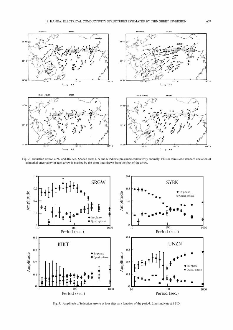
and 10 sec. The vectors at the sites indicated by closed cir-cles in Fig. 1 are estimated using the robust method (Egbertand Booker, 1986). As the magnetic variation data at the20 sites presented in Handa et al. (1992), which are in-dicated by closed squares in Fig. 1, were recorded on theold type magnetic tape, these signals, unfortunately, can-not be read now to re-calculate the transfer function usingthe robust method. In Fig. 2, plus or minus one standarddeviation of azimuthal uncertainty in each arrow is markedby the short lines drawn from the foot of the arrow. Fig-ure 3 shows the estimation errors of amplitudes for foursites where the robust method was applied. The applicationof the robust method reduces the estimation error especiallyof the quadrature-phase arrows but the errors are still largefor periods shorter than about 100 sec.

Figure 2 shows that almost all the in-phase arrows at 487sec point WSW or SW. This tendency accords well withthe previous result (Handa et al., 1992) that the arrows forlong periods are controlled mainly by the regional currentthat intensely flows into the sea. In contrast, the in-phasearrows at 97 sec are highly scattered, which implies localcomplex conductivity structures in the shallow part of thecrust: According to the fact that the in-phase arrows atboth sides of the region where high-conductivity bodies lieunderneath, point toward each other and are relatively smallnear the center, three shaded regions of high-conductivity (I,N and S) are listed in Fig. 2.

The dependence of the in-phase amplitudes on period in

S. HANDA: ELECTRICAL CONDUCTIVITY STRUCTURES ESTIMATED BY THIN SHEET INVERSION 607

Fig. 2. Induction arrows at 97 and 487 sec. Shaded areas I, N and S indicate presumed conductivity anomaly. Plus or minus one standard deviation ofazimuthal uncertainty in each arrow is marked by the short lines drawn from the foot of the arrow.

Fig. 3. Amplitude of induction arrows at four sites as a function of the period. Lines indicate ±1 S.D.

608 S. HANDA: ELECTRICAL CONDUCTIVITY STRUCTURES ESTIMATED BY THIN SHEET INVERSION

Fig. 3 also supports this tendency: The in-phase amplitudedecreases gradually with a decreasing of the period andreaches a minimum at about 120 sec, as typically seen atUNZN. This is a common response in central Kyushu, ex-cept for the eastern part where the in-phase arrows tend topoint towards the east (e.g. SRGW in Fig. 2), because theeffect of the Seto Inland Sea is rather dominant. The de-crease of amplitudes can be explained from the fact that thez-component variations of magnetic field decrease rapidlyas far from the coastline and with a decreasing period. Incontrast, the shorter-period amplitudes less than about 120sec are quite local. Thus, we will use the GDS data for pe-riods shorter than about 120 sec in the thin sheet modeling.

3. Thin Sheet ModelingIn order to obtain a conductance distribution in the shal-

low crust, the thin sheet modeling was carried out usingthese GDS data. We used a model of 94 × 94 grids witha grid-node spacing of 5 km, which is adopted on the ba-sis of the mean distance between the adjacent observationsites considering the skin depth of the layer below the thinsheet. A non-uniform thin sheet with thickness (h1) of 0.7km is assumed to be underlain by two layers; the first layer,immediately below the thin sheet, is 50 km thick with a uni-form conductivity of 0.005 S/m, and the bottom layer is ahalf-space with a conductivity of 0.01 S/m. The previousthin sheet model (Shimoizumi et al., 1997) suggests thata conductivity of 0.001 and 0.01 S/m is the crust and theupper mantle values, respectively, which best explains thelong-period arrows when only the land-sea configuration isconsidered. The resistive crust is also suggested by the MTresults observed in the Aso area (Handa et al., 1992). Al-though the value of 0.005 S/m seems to be large, we mustadopt this value to satisfy the thin sheet model conditionthat the area (470 × 470 km) should be large enough com-pared to the skin depth of the first layer (78.6 km for theperiod of 122 sec) (Agarwal and Weaver, 1989), becausethe modeling size of 94 × 94 is almost maximum for thecomputer resources.

We firstly constructed the initial thin sheet model, whichis based on the surface geology shown in Fig. 1. In thismodel, the thin sheet conductance of land is 3.5 S exceptfor the areas covered with rocks of the Chichibu belt (0.78S) between OKL and BTL in Fig. 5, granite (0.78 S), andQuaternary sediments (7 S). When the sea is shallower than700 m, conductance in the surrounding sea with depth d(m) is estimated at 4d + 0.005(700 − d), where seawateris 4 S/m and the layer beneath the sea is assumed to havea conductivity of 0.005 S/m. Conductance is assumed tobe 4d in the sea with a depth of over 700 m, which is anexceptional case in our model.

The in-phase and the quadrature arrows were calculatedfor the periods of 77, 97 and 122 sec using the thin sheettechnique (McKirdy et al., 1985). The thin sheet approxi-mation (Schmucker, 1970) requires that the thickness (h1)must be less than a third of the skin depth (δ1) in thesheet. Since the quantity of h1/δ1 increases with increas-ing conductance of the sheet, the largest value usually ap-pears in seas. The minimum period satisfying the condition(h1/δ1 < 0.3) is 69.8 sec where conductivity of the thin

sheet is 4 S/m and h1 is 0.7 km. The period is also restrictedby the area size or the grid-node spacing, as mentioned pre-viously. In this model, the maximum period is about 122sec. This is the reason why these periods were selected.

Next, we carried out the inversion adopting a conju-gate gradient relaxation method based on the procedure de-scribed by Wang and Lilley (1999). The smoothing param-eter (λ) of 4 × 10−4 is adopted, which controls the balancebetween the data misfit function L(m) and the model char-acteristic function R(m). That is, an object function () ofa model m is defined by (m) = L(m) + λR(m). Thesefunctions for this case are given as follows (Wang and Lil-ley, 1999):

L(m) = 1/2{dobs − g(m)}TC−1d {dobs − g(m)},

where C−1d is a covariance matrix describing the errors in

the observed data and dobs and g(m) are the observed dataand the calculated response, respectively.

R(m) = 1/2mT ∂Tx ∂xm + 1/2mT ∂T

y ∂ym,

where ∂x and ∂y are operators which take the differencebetween the model parameters of adjacent cells in the x andy directions, respectively. The parameter λ is less effectiveon our inversion result in the range of 0 to 1, and the valueadopted yields to the minimum misfit that is about 2 percentsmaller than the misfit for λ = 0.

The inversion was started at the initial model and we fi-nally adopted the model where the sum of the residual val-ues (misfit) is minimum. The misfit is calculated as the dataresidual parameter, defined as �|dobs − g(m)| (Wang andLilley, 1999). The sum is taken over all data that are fourcomponents for three periods at all the observation sites. Inthis process, the conductance values for the surrounding searegions were kept fixed, but for the shallow seas—that is,the Ariake Sea, the Beppu Bay, and the Tachibana Bay—changing conductance values was permitted when the in-verted values are larger than those in the initial model.

The sum of the residual values slightly decreased from47.97 to 37.02 by the inversion. The large misfit, in detailoccurs in the y-components (Bu and Bv): The residues forBu and Bv change from 12.45 to 11.37 and from 9.37 to9.03, respectively, while that for Au successfully decreasesfrom 18.33 to 8.7. This y-component misfit is possiblycaused by the land-sea configuration in our model. Thethin-sheet modeling method in this study prohibits verti-cal current leakage, which depresses the transfer functionsparticularly near coastlines (Kuvshinov et al., 1999). Thus,some misfits are caused by this restriction in the eastern andwestern areas near the coastline. However, as the large mis-fits are even found in the central part, the following causesshould be considered in this case. As the current flow in theNS direction, which is induced by geomagnetic field varia-tions concentrates in the East China Sea, the current densityis relatively low in central Kyushu, while the EW currentis not so strongly, governed by the land-sea configuration.Thus, the conductance perturbations on land can cause therelatively small change of the Bu value in the inversion pro-cess. This is clearly shown in Fig. 4: the sensitivity of Buto normalized conductance (McKirdy et al., 1985) perturba-tions in the cell is about a third of others. For these reasons,

S. HANDA: ELECTRICAL CONDUCTIVITY STRUCTURES ESTIMATED BY THIN SHEET INVERSION 609

Fig. 4. The sensitivity to conductance perturbations in the cell of Au, v and Bu, v data at the central cell (KIKT) marked by a circle. Sensitivity mapsare shown for the period of 97 sec.

Fig. 5. The final thin sheet model. Triangles show active volcanoes. BKF: Beppu-Kita fault, BTL: Butsuzo tectonic line, HHL: Hita-Hakuso tectonicline, MIL: Matsuyama-Imari tectonic line, OKL: Oita-Kumamoto tectonic line, UYL: Usuki-Yatsushiro tectonic line.

the reduction of the misfit in the y-component of the trans-fer function is difficult only through this inversion process.

Moreover, another limitation of this model is seen inFig. 4: an ‘effective sensitivity range’ that is the distancein which a sensitivity value decays to half of its maximum

value (Wang and Lilley, 1999) is a radius of one cell. Thismean that only the conductance perturbation at the adjacentcells can effectively change the transfer functions and theflexibility of modeling is poor. Grid-spacing shorter than5 km should be assigned to avoid this problem, but that is

610 S. HANDA: ELECTRICAL CONDUCTIVITY STRUCTURES ESTIMATED BY THIN SHEET INVERSION

Fig. 6. Response of in-phase and quadrature induction arrows for 97 sec., which are calculated for the initial and the final models. Observed arrows areindicated by thick lines.

difficult because of the limitation of the thin sheet condition,as mentioned before.

In order to overcome these problems, the trial and errormodeling technique was applied after inverting the initialmodel, and then the inversion was made again. By thisprocedure, the total residue finally decreased to 23.7. Theaverage residue for a component at a site is 0.026. Thisinverted conductance distribution (the final model) is shownin Fig. 5. The in-phase and the quadrature arrows calculatedfor the initial and the final models are shown in Fig. 6 alongwith those observed for the period of 97 sec. The arrowsfor 77 and 122 sec are not shown here because they aresimilar to those in Fig. 6. Comparing these figures in Fig. 6,it is found that the misfit improves for the in-phase arrows,while there are still some misfits of the quadrature-phasearrow mainly due to the relatively large estimation errorscaused by cultural noises.

4. DiscussionThe conductive areas with enhanced conductance of

more than 10 S after the inversion process are illustratedin Fig. 7 for convenience of the following discussion. Wewill discuss three relatively broad areas marked by B, S andU, which include the high-conductivity areas expected fromthe induction arrow data in Fig. 2.4.1 High-conductive alluvial plain

The main part of the conductive area ‘S’ covers theSaga-Chikugo plain. This high conductivity is probably

due to alluvium with a thickness of about 200 m; in theSaga-Chikugo plain, unconsolidated sediments includingthe ‘Ariake clay’ are underlain by Palaeogene sediments.The Ariake clay, which lies near the ground surface witha thickness of several meters, is quite high-conductive andthe surface layer including Ariake clay has a resistivity inthe range from 5 to 25 -m. This implies that conductorsmuch thinner than the skin depth can intensely affect theinduction arrows by concentrating the induced current intosuch areas, as Nishida (1976) pointed out in the GDS studyof southern Hokkaido.4.2 Conductivity structures in the BSG

The area ‘B’ is the most conductive region. The conduc-tive belt ‘M’ from Beppu Bay to the west along MIL andBKF (Fig. 2) is suggested from the observed induction ar-rows. The final model indicates that the high-conductivityzones are found in this area along almost all the tectoniclines; MIL, BKF, OKL and possibly UYL. These tectoniclines are not only traced by the high-conductivity belt butalso the border of a high-conductive triangular region of theHohi volcanic zone.

The Hohi volcanic zone is characterized by a ‘box-shaped negative anomaly’ (Kamata, 1989) as seen in thecontour map of the Bouguer anomaly in Fig. 7. The gravi-metric analysis and drill hole data indicate that the pre-Tertiary basement is a half-graben structure filled with vol-canic formations: the cross-section along the line AB (Ka-mata, 1993) is shown in Fig. 8, in which a maximum depth

S. HANDA: ELECTRICAL CONDUCTIVITY STRUCTURES ESTIMATED BY THIN SHEET INVERSION 611

Fig. 7. Tectonic interpretation of the electrical conductivity model in central Kyushu. The enhanced conductance values compared with the initial modelare indicated. The region surrounded by a broken line indicates Quaternary sediments of the Saga-Chikugo plain. The Bouguer gravity anomaly isshown by thin lines with an interval of 20 mgals, which is compiled from Geological Survey of Japan (2002a and b). The shallow structure ofthe graben is shown along line AB in Fig. 8. Triangles indicate active volcanoes. BKF: Beppu-Kita fault, HHL: Hita-Hakuso tectonic line, MIL:Matsuyama-Imari tectonic line, OKL: Oita-Kumamoto tectonic line, UYL: Usuki-Yatsushiro tectonic line.

10 100 1000 Ω-m

volcanic rocks

pre-Tertiary basement rocks

1

0

-1

-2

-3

-4 0 5 10 km

kmA BOKL Tsurumi BKF

SSE NNW

Fig. 8. The graben structure estimated from the gravimetric data and the 2-D conductivity model along AB, compiled from Kamata (1993) and NEDO(1989), respectively.

of 5 km appears at the north of OKL and the basement risesgradually in its northern part. The 2-D electrical conduc-tivity structure (NEDO, 1989) is also shown in this figure,which is obtained by the long-period MT and the CSAMTdata that is along the line at about 1 km east and roughlyparallel to the line AB. This model implies that the shallowpart of volcanic formations within the graben is highly con-ductive and underlain by a resistive layer of 1000 ohm-m,and the basement is not clarified in contrast to the structureestimated from the gravimetric data.

The correlation is good between the shallow part of the2-D conductivity structure and our final model: For exam-ple, a high-conductive zone across the line AB at the im-mediately north of OKL is seen in the thin sheet model,which possibly corresponds to the most conductive layer

of 10 ohm-m at the same position in the 2-D model. Thisimplies that the thin sheet model reveals conductive layersshallower than about 1 km depth at least around the line ABand possibly in all the B area.

The BSG occupies the eastern region of the Hohi vol-canic zone. This is a tectonically active zone: The sur-face geology indicates that many normal-type faults withthe east-west strike are well developed and form the Beppugraben. In the Beppu bay where conductivity is high, mul-tichannel seismic reflection and gravity surveys delineatedseveral faults in the sedimentary layer covering the de-pressed basement that undulates within a few thousand me-ters (Yusa et al., 1992). Also, geothermal activity is high,as is evident from hot water springs and fumaroles in theB area. These imply a close relation between the high-

612 S. HANDA: ELECTRICAL CONDUCTIVITY STRUCTURES ESTIMATED BY THIN SHEET INVERSION

conductivity structure including the zone along the tectoniclines and geothermal system, because high-conductivity inthe shallow crust is frequently caused by geothermal activ-ity.

In a western area of central Kyushu, the narrow high-conductivity zone is expected from the anti-parallelism ofin-phase arrows in the root of the Shimabara peninsula (Nin Fig. 2). The inverted result, however, indicates that theconductive region is spread out widely; the BSG and thezone between the OKL and UYL. In the peninsula, the Un-zen graben runs across the central part in the EW directionand the Unzen active volcano stands within the graben. Theshallow conductive layer that can explain high-conductivityof the thin sheet model is also found in this area: The MTsurvey in the peninsula indicates that the extremely con-ductive layer of a few ohm-m at a depth of about 1 to 2 kmlies between the highly resistive surface layer and a layer ofabout 100 ohm-m (Yamamoto et al., 1996).

The conductive zone of the western BSG is bounded onthe east by the Aso area which is resistive, as seen in Fig. 7,and the BSG seems to be discontinuous in the shallow elec-trical structure. In this high-resistive area, no clear fault sys-tem of the graben is found by the surface geology. Althoughthe negative gravity anomaly that is the most important ev-idence of the BSG is found in this area, it does not indicatethe graben but the caldera structure that is filled with lightermaterials ejected by eruptions of the Aso volcano. Thus,the central portion is tectonically different from the otherareas and the BSG is possibly separated into three parts inthe shallow electrical structure; the high-conductive easternand western zones and the resistive central area.

5. ConclusionThe conductivity structure in the shallow crust of central

Kyushu is clarified by the thin sheet inversion method us-ing the GDS data set for the periods of 77, 97 and 122 sec.In the modeling process, the fitness of the y-component inthe in-phase transfer functions is not easily improved onlyby the inversion method, because of the land-sea configu-ration in this model: as current flow in the NS directionconcentrates in the East China Sea, the sensibility of the y-component transfer functions to conductance perturbationsat a cell on land is about a third of the others. This can beovercome by partly applying the trial and error method andthe fit of the model finally obtained is sufficient.

The inverted model reveals that the high-conductive ar-eas distributed widely in central Kyushu; the Chikugo-Sagaalluvial plain and the eastern and the western areas includ-ing the BSG. The MT results imply that the conductivitymap obtained represents the distribution of the conductivelayers shallower than about 1 km. The eastern and thewestern parts of the BSG, which are the tectonically ac-tive zones in Beppu and the Shimabara peninsula, are in-tensely conductive. These conductive areas are not local-ized only in the BSG but also found in the zone betweentwo tectonic lines of OKL and UYL in the Shimabara areaand in the Hohi volcanic zone. In the Beppu area, the high-conductivity zones are found along the tectonic lines bound-ing the BSG. In contrast, the central part of the BSG is re-sistive, in which no clear graben structure is found by the

surface geology. Thus, the BSG is not revealed as a con-tinuous high-conductive belt and it is separated into threeparts. That is the eastern and the western high-conductivezones and the resistive central area in the electrical conduc-tivity model.

Acknowledgments. I would like to express my thanks to Dr. H.Toh for providing the computer program of the thin sheet calcula-tion. Constructive reviews by Dr. S. G. Gokarn and the anonymousreviewers significantly improved the manuscript.

ReferencesAgarwal, A. K. and J. T. Weaver, Regional electromagnetic induction

around the Indian peninsula and Sri Lanka; a three dimensional numeri-cal study using the thin sheet approximation, Phys. Earth Planet. Inter.,54, 320–331, 1989.

Editorial Committee of Kyushu, Part 9 of Regional Geology of Japan,Regional Geology of Japan Part 9 Kyushu, 371 pp., Kyoritsu Shuppan,Tokyo, 1992.

Egbert, E. D. and J. R. Booker, Robust estimation of geomagnetic transferfunctions, Geophy. J. R. Astr. Soc., 87, 173–194, 1986.

Eguchi, T. and S. Uyeda, Seismotectonics of the Okinawa Trough andRyukyu Arc, Mem. Geol. Soc. China, 5, 189–210, 1983.

Geological Survey of Japan, Gravity map of Fukuoka district (Bougueranomaly), Geol. Surv. Japan, 2002a.

Geological Survey of Japan, Gravity map of Ooita district (Bougueranomaly), Geol. Surv. Japan, 2002b.

Handa, S., Y. Tanaka, and A. Suzuki, The electrical high conductivitylayer beneath the northern Okinawa Trough, inferred from geomagneticdepth sounding in Northern and Central Kyushu, Japan, J. Geomag.Geoelectr., 44, 505–520, 1992.

Kamata, H., Volcanic and structural history of the Hohi volcanic zone,central Kyushu, Japan, Bull. Volcanol., 51, 315–332, 1989.

Kamata, H., Subsurface geologic structure and its genesis of Beppu Bayand adjacent area in central Kyushu, Japan, J. Geol. Soc. Japan, 99, 39–46, 1993 (in Japanese with English abstract).

Kuvshinov, A. V., D. B. Avdeev, and O. V. Pankratov, Global induction bySq and Dst sources in the presence of oceans: bimodal solutions for non-uniform spherical surface shells above radially symmetric earth modelsin comparison to observations, Geophys. J. Int., 137, 630–650, 1999.

Matsumoto, Y., Some problems on the volcanic activities and depressionstructures in Kyushu, Japan, Mem. Geol. Soc. Japan, 16, 127–139, 1979(in Japanese).

McKirdy, D. McA., J. T. Weaver, and T. W. Dawson, Induction in a thinsheet of variable conductance at the surface of a stratified earth—II.Three-dimensional theory, Geophy. J. R. Astr. Soc., 80, 177–194, 1985.

Nakada, T. and H. Kamata, Temporal change in chemistry of magmasource under Central Kyushu, Southwest Japan: progressive contami-nation of mantle wedge, Bull. Volcanol., 53, 195–206, 1991.

NEDO, Report of the resistively survey (MT and CSAMT) in the Tsurumi-Dake area, NEDO, 1989 (in Japanese).

Nishida, Y., Conductivity anomalies in the southern half of Hokkaido,Japan, J. Geomag. Geoelectr., 28, 375–394, 1976.

Parkinson, W. D., The influence of continents and oceans on geomagneticvariation, Geophys. J., 6, 441–449, 1962.

Schmucker, U., Anomalies of geomagnetic variations in the southwesternUnited States, Bull. Scripps Inst., 13, Univ. of Calif. Press, 1970.

Shimoizumi, M., T. Mogi, M. Nakada, T. Yukutake, S. Handa, Y. Tanaka,and H. Utada, Electrical conductivity anomalies beneath the western seaof Kyushu, Japan, Geophys. Res. Lett., 24, 1551–1554, 1997.

Wang, L. J. and F. E. M. Lilley, Inversion of magnetometer array data bythin-sheet modelling, Geophys. J. Int., 137, 128–138, 1999.

Yamamoto, T., T. Kagiyama, and H. Utada, Resistivity structure by ULF-MT around Unzen Volcano, SW Japan, 13th Workshop on Electromagn.Ind. In the Earth, 1996.

Yusa, Y., K. Takemura, K. Kitaoka, K. Kamiyama, S. Horie, I. Nakagawa,Y. Kobayashi, A. Kubotera, Y. Sudo, T Ikawa, and M. Asada, Subsur-face structure of Beppu Bay (Kyushu, Japan) by seismic reflection andgravity survey, Zisin, 45, 199–212, 1992 (in Japanese with English ab-stract).

S. Handa (e-mail: handas@cc.saga-u.ac.jp)