Efficiency and Q for small antennas using Pareto optimality

Efficiency and Q for small antennas usingPareto optimality

Mats Gustafsson(Marius Cismasu, Sven Nordebo)

Department of Electrical and Information Technology

Lund University, Sweden

IEEE-APS, Orlando, USA, July 8, 2013

Design of small antennas

Folded spherical helix SonyEricsson P1i Fragmented patches

I There are many advanced methods to design small antennas.I Often antennas embedded in structures.I Performance in Q, bandwidth and efficiency.I Fundamental tradeoff between Q and size (and bandwidth for

passive matching).I A figure of merit for performance.I What about efficiency?

Mats Gustafsson, Department of Electrical and Information Technology, Lund University, Sweden

Tradeoff between performance and size

I Radiating (antenna) structure, V .

I Antenna volume, V1 ⊂ V .

I Current density J1 in V1.

I Radiated field, F (k), in direction kand polarization e.

Questions analyzed here, J1 for:

I maximum G(k, e)/Q.

I superdirectivity.

I embedded antennas.

I efficiency.

I also minimum Q for given radiatedfields, sidelobe levels, MIMO...

VV1

y

x

z

k

e

^


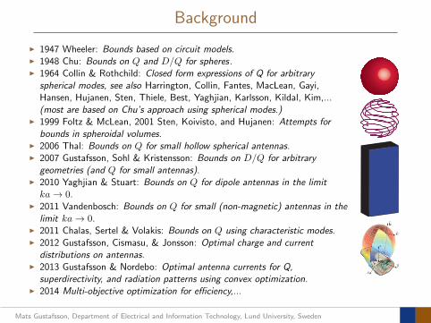
Background

I 1947 Wheeler: Bounds based on circuit models.I 1948 Chu: Bounds on Q and D/Q for spheres.I 1964 Collin & Rothchild: Closed form expressions of Q for arbitrary

spherical modes, see also Harrington, Collin, Fantes, MacLean, Gayi,Hansen, Hujanen, Sten, Thiele, Best, Yaghjian, Karlsson, Kildal, Kim,...(most are based on Chu’s approach using spherical modes.)

I 1999 Foltz & McLean, 2001 Sten, Koivisto, and Hujanen: Attempts forbounds in spheroidal volumes.

I 2006 Thal: Bounds on Q for small hollow spherical antennas.I 2007 Gustafsson, Sohl & Kristensson: Bounds on D/Q for arbitrary

geometries (and Q for small antennas).I 2010 Yaghjian & Stuart: Bounds on Q for dipole antennas in the limitka→ 0.

I 2011 Vandenbosch: Bounds on Q for small (non-magnetic) antennas in thelimit ka→ 0.

I 2011 Chalas, Sertel & Volakis: Bounds on Q using characteristic modes.I 2012 Gustafsson, Cismasu, & Jonsson: Optimal charge and current

distributions on antennas.I 2013 Gustafsson & Nordebo: Optimal antenna currents for Q,

superdirectivity, and radiation patterns using convex optimization.I 2014 Multi-objective optimization for efficiency,...

VV1

y

x

z

k

e

^


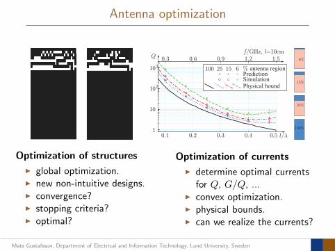
Antenna optimization

0.1 0.2 0.3 0.4 0.5 l/¸

10

102

1

Q

103

0.3 0.6 0.9 1.2 1.5f/GHz, l=10cm

61525

SimulationPrediction

Physical bound

% antenna region100

6%

15%

25%

100%

Optimization of structures

I global optimization.I new non-intuitive designs.I convergence?I stopping criteria?I optimal?

Optimization of currents

I determine optimal currentsfor Q, G/Q, ...

I convex optimization.I physical bounds.I can we realize the currents?


Antenna optimization

l/¸=0.1 l/¸=0.25l/¸=0.175

0.1 0.2 0.3 0.4 0.5 l/¸

10

102

1

Q

103

0.3 0.6 0.9 1.2 1.5f/GHz, l=10cm

61525


Physical bound

% antenna region100

6%

15%

25%

100%

Optimization of structures

I global optimization.I new non-intuitive designs.I convergence?I stopping criteria?I optimal?

Optimization of currents

I determine optimal currentsfor Q, G/Q, ...

I convex optimization.I physical bounds.I can we realize the currents?


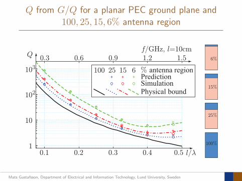
Q from G/Q for a planar PEC ground plane and100, 25, 15, 6% antenna region

0.1 0.2 0.3 0.4 0.5 l/¸

10

102

1

Q

103

0.3 0.6 0.9 1.2 1.5f/GHz, l=10cm

61525


Physical bound

% antenna region100

6%

15%

25%

100%


Optimization of antenna current

Gain over Q

minimize Stored energy

subject to Radiation intensity = P0

Q for superdirectivity D ≥ D0.


subject to Radiation intensity = D0Prad/(4π)

Radiated power ≤ Prad

Embedded structures


subject to Radiation intensity = P0

Correct induced currents

VV1

y

x

z

k

e

^


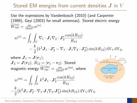
Stored EM energies from current densities J in V

Use the expressions by Vandenbosch (2010) (and Carpenter(1989), Geyi (2003) for small antennas). Stored electric energy

W(e)vac = µ0

16πk2w(e)

w(e) =

∫V

∫V∇1 · J1∇2 · J∗2

cos(kR12)

R12

− k

2

(k2J1 · J∗2 −∇1 · J1∇2 · J∗2

)sin(kR12) dV1 dV2,

J(r)

E(r), H(r)

electric current density

near field

far field

induced EM field

²=²0¹=¹0

(reactive and radiated fields)

(radiated field)

where J1 = J(r1),J2 = J(r2), R12 = |r1 − r2|. Stored

magnetic energy W(m)vac = µ0

16πk2w(m), where

w(m) =

∫V

∫Vk2J1 · J∗2

cos(kR12)

R12

−k2

(k2J1·J∗2−∇1·J1∇2·J∗2

)sin(kR12) dV1 dV2.


Stored EM energies from current densities J in V II

Also the total radiated power Prad = η08πkprad with

prad =

∫V

∫V

(k2J1 · J∗2 −∇1 · J1∇2 · J∗2

)sin(kR12)

R12dV1 dV2.

Method of Moments approximation (expand J in basis functions)

w(e) ≈ JHXeJ stored E-energy

w(m) ≈ JHXmJ stored M-energy

prad ≈ JHRrJ radiated power

We also use

F ≈ FHJ far field

J2 ≈ Z′J1 induced current on a PEC

The normalized quantities w(e), w(m), and prad have dimensionsgiven by volume, m3, times the dimension of |J |2.


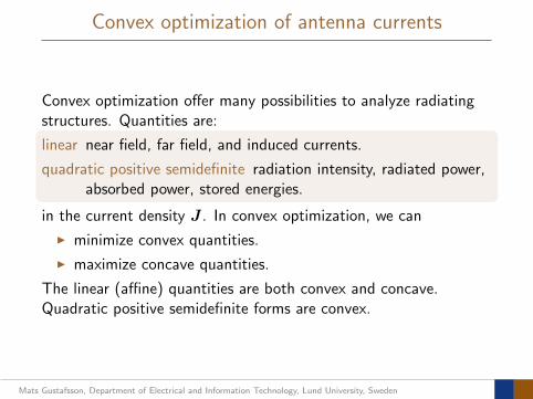
Convex optimization of antenna currents

Convex optimization offer many possibilities to analyze radiatingstructures. Quantities are:

linear near field, far field, and induced currents.

quadratic positive semidefinite radiation intensity, radiated power,absorbed power, stored energies.

in the current density J . In convex optimization, we can

I minimize convex quantities.

I maximize concave quantities.

The linear (affine) quantities are both convex and concave.Quadratic positive semidefinite forms are convex.


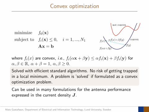
Convex optimization

minimize f0(x)

subject to fi(x) ≤ 0, i = 1, ..., N1

Ax = b

convex

not convex

f(y)

f(x)

f(®x+¯y)

®f(x)+¯f(y)

where fi(x) are convex, i.e., fi(αx + βy) ≤ αfi(x) + βfi(y) forα, β ∈ R, α+ β = 1, α, β ≥ 0.

Solved with efficient standard algorithms. No risk of getting trappedin a local minimum. A problem is ’solved’ if formulated as a convexoptimization problem.

Can be used in many formulations for the antenna performanceexpressed in the current density J .


Currents for maximal G/Q for embedded antennas

Determine an optimal current density J1(r) in the volume V1. Assumethat V is PEC outside V1.Can minimize the stored energy for givenradiated field

minimize maxJHXeJ,JHXmJ

subject to ReFHJ = 1

J2 = Z′J1

or maximize the radiated field for givenstored energy

maximize ReFHJsubject to JHXeJ ≤ 1

JHXmJ ≤ 1

J2 = Z′J1

Can also eliminate J2.

VV1

y

x

z

k

e

^


Embedded antennas in planar PEC rectangles

1

10

100

1000

` /¸x

Q

0.1 0.2 0.3 0.4 0.5

x

y z

^

^ ^

` /2 x

` xa

V2

V1

PEC

»` x

»` /2 x

»=0.5

»=0.25

»=0.5

»=1

»=0.25


D/Q (or G/Q) bounds

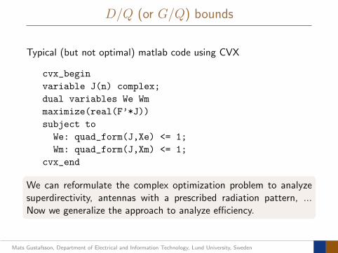
Typical (but not optimal) matlab code using CVX

cvx_begin

variable J(n) complex;

dual variables We Wm

maximize(real(F’*J))

subject to

We: quad_form(J,Xe) <= 1;

Wm: quad_form(J,Xm) <= 1;

cvx_end

We can reformulate the complex optimization problem to analyzesuperdirectivity, antennas with a prescribed radiation pattern, ...Now we generalize the approach to analyze efficiency.


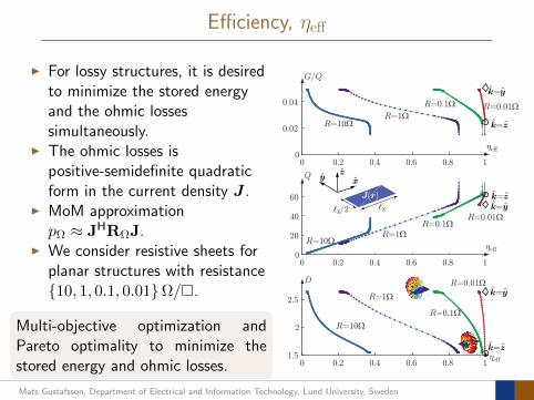
Efficiency, ηeff

I For lossy structures, it is desiredto minimize the stored energyand the ohmic lossessimultaneously.

I The ohmic losses ispositive-semidefinite quadraticform in the current density J .

I MoM approximationpΩ ≈ JHRΩJ.

I We consider resistive sheets forplanar structures with resistance10, 1, 0.1, 0.01Ω/.

Multi-objective optimization andPareto optimality to minimize thestored energy and ohmic losses.

0 0.2 0.4 0.6 0.8 10

0.02

0.04

0 0.2 0.4 0.6 0.8 10

20

40

60

0 0.2 0.4 0.6 0.8 11.5

2

2.5

G/Q

Q

D

éff

éff

éff

` x` /2x

J(r)

xyz

^^ ^

k=y^

k=z^

R=0.01Ω

R=0.1Ω

R=1Ω

R=10Ω

R=0.01ΩR=0.1ΩR=1Ω

R=10Ω

R=0.01ΩR=0.1Ω

R=1ΩR=10Ω

k=z^

k=z^

k=y^

k=y^


Efficiency, ηeff , using Pareto optimality

Linear combination of the storedenergy and ohmic losses

min. αmaxJHXeJ,JHXmJ

+ (1− α)JHPΩJ

s.t. ReFHJ = 1

where + ≤ α ≤ 1. A planarrectangle with side lengths `x and`x/2 modeled as a resistive sheetwithR = 1/(σd) = 10, 1, 0.1, 0.01Ω/is used to illustrate the tradeoffbetween Q, D, and ηeff for`x/λ ≈ 0.13 (or ka ≈ 0.44).

0 0.2 0.4 0.6 0.8 10

0.02

0.04

0 0.2 0.4 0.6 0.8 10

20

40

60

0 0.2 0.4 0.6 0.8 11.5

2

2.5

G/Q

Q

D

éff

éff

éff

` x` /2x

J(r)

xyz

^^ ^

k=y^

k=z^

R=0.01Ω

R=0.1Ω

R=1Ω

R=10Ω

R=0.01ΩR=0.1ΩR=1Ω

R=10Ω

R=0.01ΩR=0.1Ω

R=1ΩR=10Ω

k=z^

k=z^

k=y^

k=y^


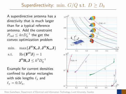
Superdirectivity: min. G/Q s.t. D ≥ D0

A superdirective antenna has adirectivity that is much largerthan for a typical referenceantenna. Add the constraintPrad ≤ 4πD−1

0 the get theconvex optimization problem

min. maxJHXeJ,JHXmJ

s.t. ReFHJ = 1

JHRrJ ≤ k3D−10

Example for current densitiesconfined to planar rectangleswith side lengths `x and`y = 0.5`x.

0.1 0.2 0.3 0.4 0.51

10

100

103Q

` x` /2x

J(r)

xyz

^^ ^

` /¸x

D(x)=9^

7

5

3

0 0.2 0.4 0.6 0.8 110

2

103

104 Q

D(x)=9^7

5

3

´eff


Superdirectivity: min. G/Q s.t. D ≥ D0

Linear combination for losses:

min. αW + (1− α)JHPΩJ

s.t. JHXeJ ≤WJHXmJ ≤WReFHJ = 1

JHRrJ ≤ k3D−10

Example for current densitiesconfined to planar rectangleswith side lengths `x and`y = 0.5`x, R = 0.01 Ω/,and ka = 0.44.

0.1 0.2 0.3 0.4 0.51

10

100

103Q

` x` /2x

J(r)

xyz

^^ ^

` /¸x

D(x)=9^

7

5

3

0 0.2 0.4 0.6 0.8 110

2

103

104 Q

D(x)=9^7

5

3

´eff


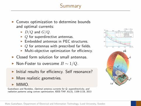
Summary

I Convex optimization to determine boundsand optimal currents:

I D/Q and G/Q.I Q for superdirective antennas.I Embedded antennas in PEC structures.I Q for antennas with prescribed far fields.I Multi-objective optimization for efficiency.

I Closed form solution for small antennas.

I Non-Foster to overcome B ∼ 1/Q.

I Initial results for efficiency. Self resonance?

I More realistic geometries.

I MIMO.Gustafsson and Nordebo, Optimal antenna currents for Q, superdirectivity, andradiation patterns using convex optimization, IEEE-TAP, 61(3), 1109-1118, 2013

0.1 0.2 0.3 0.4 0.5 l/¸

10

102

1

Q

103

0.3 0.6 0.9 1.2 1.5f/GHz, l=10cm

61525


Physical bound

% antenna region100

VV1

y

x

z

k

e

^


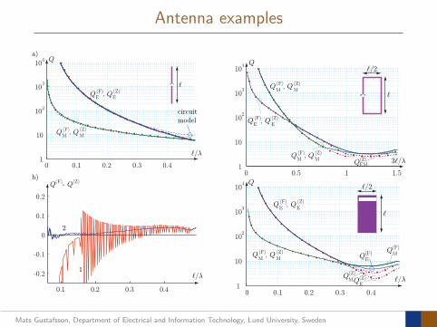
Antenna examples

0.1 0.2 0.3 0.4

-0.2

-0.1

0

0.1

0.2

0 0.1 0.2 0.3 0.41

10

10

103

104

Q - Q(F) (Z)

1

2

Q

`/¸

`/¸

a)

b)

2circuitmodel

`

Q , Q(F) (Z)E

Q , Q(F) (Z)

M M

E

0 0.5 1 1.51

10

102

103

104 Q

3`/¸Q (Z)

`/2

`Q , Q(F) (Z)

M M

Q , Q(F) (Z)

E E

EM

Q , Q(F) (Z)

M M

1

10

102

103

104 Q

`/¸

`

0 0.1 0.2 0.3 0.4

`/2

Q (F)E

Q (F)M

Q (Z)

Q , Q(F) (Z)E

Q , Q(F) (Z)

M M

Q (Z)E

E

M


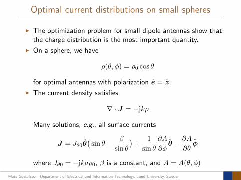
Optimal current distributions on small spheres

I The optimization problem for small dipole antennas show thatthe charge distribution is the most important quantity.

I On a sphere, we have

ρ(θ, φ) = ρ0 cos θ

for optimal antennas with polarization e = z.

I The current density satisfies

∇ · J = −jkρ

Many solutions, e.g., all surface currents

J = Jθ0θ(

sin θ − β

sin θ

)+

1

sin θ

∂A

∂φθ − ∂A

∂θφ

where Jθ0 = −jkaρ0, β is a constant, and A = A(θ, φ)


Optimal current distributions on small spheres

Some solutions:

I Spherical dipole,β = 0, A = 0.

I Capped dipole,β = 1, A = 0.

I Folded spherical helix,β = 0, A 6= 0.

They all have almost identicalcharge distributions

ρ(θ, φ) = ρ0 cos θ

Can mathematical solutionssuggest antenna designs?

−3

−2.5

−2

−1.5

−1

−0.5

0

0 45 90 135 1800

0.2

0.4

0.6

0.8

1

45 90 135 180

−1

−0.5

0

0.5

1

a)

b)

c)

J /Jµ0µ

± ± ± ± ±µ

45 90 135 180± ± ± ±µJ /Jµ0µ

J/Jµ0

Á

µ

± ± ± ±


Efficiency and Q for small antennas using Pareto optimality

Documents

Transcript of Efficiency and Q for small antennas using Pareto optimality