On cone based decompositions of proper Pareto optimality · On cone based decompositions of proper...

Noname manuscript No.(will be inserted by the editor)

On cone based decompositions of proper Paretooptimality

Marlon A. Braun · Pradyumn K.Shukla · Hartmut Schmeck

Received: date / Accepted: date

Abstract In recent years, the research focus in multi-objective optimizationhas shifted from approximating the Pareto optimal front in its entirety to iden-tifying solutions that are well-balanced among their objectives. Proper Paretooptimality is an established concept for eliminating Pareto optimal solutionsthat exhibit unbounded tradeoffs. Imposing a strict tradeoff bound allows spec-ifying how many units of one objective one is willing to trade in for obtainingone unit of another objective. This notion can be translated to a dominancerelation, which we denote by M-domination. The mathematical properties ofM-domination are thoroughly analyzed in this paper yielding key insights intoits applicability as decision making aid. We complement our work by provid-ing four different geometrical descriptions of the M-dominated space given bya union of polyhedral cones. A geometrical description does not only yield agreater understanding of the underlying tradeoff concept, but also allows aquantification of the space dominated by a particular solution or an entire setof solutions. These insights enable us to formulate volume-based approachesfor finding approximations of the Pareto front that emphasize regions that arewell-balanced among their tradeoffs in subsequent works.

Keywords multi-objective optimization · proper Pareto optimality · conedomination · polyhedral cones · hypervolume

Nomenclature

A l ×m matrix where l ∈ NAoσ Matrix of the ordered objectives approach using permutation σ

M. Braun, P. Shukla, H. SchmeckInstitut AIFB - Geb. 05.20 KIT-Campus Sud, 76128 KarlsruheTel.: +49 721 608-46591E-mail: marlon.braun, pradyumn.shukla, [email protected]

2 Marlon A. Braun et al.

Asij Matrix of the simplified ordered objectives approach with maximumobjective difference i and minimum difference j

Amini Matrix of the minimum matrix approach of objective iC(A) Polyhedral cone induced by matrix Ad Vector in Rm used to model directions as difference between two vec-

torsdist A function for calculating the distance between two elements in the

vector space RmC(A) Cone dominance relation according to the cone C induced by matrix

AM M-domination relation according to the tradeoff level Mp Pareto dominance relationf Vector of objective functionsI Set of objective indices, i.e. I = 1, . . . ,mM Variable denoting a maximum allowed tradeoff boundm Number of objectivesn Number of decision variablesr A reference point for calculating the size of the M-dominated space of

an element in RmDM (u) Subspace of Rm that is M-dominated by uPM (u) Subspace of Rm that M-dominates uNM (u) Subspace of Rm that is non-M-dominated to uu,v,w Variables depicting values in Rmx,y, z Variables depicting values in RnX Search spaceXp Set of Pareto optimal solutionsY Objective spaceYp Image of the set of Pareto optimal points in the objective space

1 Introduction and motivation

Multi-objective optimization aims at finding solutions to problems that featuremultiple conflicting goals. In general, these problems exhibit no single solutionthat optimizes all objectives at the same time. Instead, we obtain a set ofPareto optimal solutions that forms a so-called Pareto optimal front in theobjective space. A Pareto optimal solution can only be improved in one goalby deteriorating another objective at the same time [9,8,14,21].

However, not all Pareto optimal solutions are equally attractive. Some solu-tions might only excel in one aim and suffer from highly undesirable objectivevalues in other goals. For this reason, many different notions have been pro-posed in the literature to identify preferable subsets of the Pareto front [6,4,10,7,24,16]. The concept of proper Pareto optimality [15] uses tradeoffs todescribe the desirability of a solution. A tradeoff specifies how much it costsin quantities of one objective to attain a certain gain in another goal. It was

On cone based decompositions of proper Pareto optimality 3

suggested in [23] to impose a maximum allowed deterioration-improvement-ratio to crop the set of Pareto optimal solutions, i.e. if attaining an improve-ment in one objective exceeds trading in a given quantity in some other goal,this particular solution is discarded. Subsequent works [25] have applied thisnotion to define a dominance relation, namely U-domination, by imposing adeterioration-improvement-ratio of strictly one, i.e. a solution U-dominates an-other solution, if its maximum gain exceeds the largest absolute loss comparedover all objectives. In this paper, we relax the strict exchange rate allowinglarger tradeoff bounds for defining the notion of M-domination.

The concept of M-domination allows us to focus our search efforts fromthe beginning on preferred subsets of the Pareto optimal front. We can definea threshold for obtaining solutions that only present equitable options andthereby save computational resources. Limiting the search on subsets of thePareto front has a very practical reason. Pareto fronts of most real-world prob-lems are hypersurfaces. Attaining a closed form description is often arduousand sometimes even infeasible [13,17,26,28]. For this reason, multi-objectiveoptimization algorithms try to approximate the Pareto front by a finite set ofpoints. In practical applications however, a decision maker is usually requiredto implement only a single solution. Having a multitude of possible optionsat hand burdens the decision making process. This problem can be alleviatedby cropping the Pareto front to a subset of solutions that all adhere to somedesirability criterion [5]

The question remains how the remaining subset of the Pareto front shouldbe optimally approximated, since these subsets may become rather small com-pared to the complete front or form disconnected patches [7]. For this reason,traditional techniques such as crowding distance [12], nearest neighbor selec-tion [33], decomposition methods [31] or reference point models [11] appearto be inappropriate. Previous approaches [27,7] have treated all solutions be-low the threshold equally. We want to measure the space M-dominated bya set of solutions in the objective space instead. Volume-based methods forcomputing optimal distributions of solutions on the Pareto front have beensuccessfully applied and seen increasing research interest in recent years [2,1]. A distribution of points that maximizes the volume of the M-dominatedspace would constitute a highly desirable approximation of the Pareto frontaccording to the M-domination notion. Although we propose no such algo-rithm in this paper, we lay the theoretical foundation for implementing it infuture works.

We choose to decompose the M-dominated space into polyhedral cones.Polyhedral cones are a well-known concept in multi-objective optimization todescribe preferences that generalize Pareto domination [30]. Quantifying thespace M-dominated by a set of points is a non-trivial task. Dividing the M-dominated space into polyhedral cones, however, allows us to reuse existingalgorithms that are founded on the Pareto domination principle [3,29]. Wepropose four different decomposition techniques in this work and present anextensive discussion about their applicability in practical algorithms.

We list the key contributions of our work:


– we propose a new tradeoff-based dominance concept in M-domination thatis founded on the notion of proper Pareto optimality. It is shown thatM-domination is a generalization of Pareto domination;

– an in-depth analysis of the mathematical properties of M-domination isprovided that elaborate on its applicability in a practical context;

– we provide four cone based decompositions of M-domination. Thereby wegain a deeper understanding of the underlying preference notion and obtainthe possibility to quantify the space M-dominated by a particular point.This allows the conception of volume-based optimization algorithms infuture works.

The remainder of the paper is structured as follows. In the next section,we provide a primer on some key multi-objective optimization concepts. After-wards, we present the notion of M-domination and provide an in-depth analysisof its mathematical properties. Cone based decompositions of M-dominationare explored in the subsequent section. We conclude our work by some finalremarks and an outlook on future work.

2 Multi-objective optimization concepts

Without loss of generality, we restrict our analysis to minimization problems.We consider the minimization of m objective functions f(x) := (f1(x), . . .,fm(x)) using n decision variables x := (x1, . . . , xn).

Definition 1 (Multi-objective optimization problem [9,8,14,21]) Letf(x) : Rn → Rm and X ⊆ Rn be given. The multi-objective optimizationproblem is defined as follows:

minx

f(x) := (f1(x), f2(x), . . . , fm(x)) s.t. x ∈ X. (1)

The set X (in Definition 1) is the feasible set and may be described byany number of inequalities, equalities or box constraints. Our analysis is notaffected by the composition of X. Y = f(X) denotes the objective space.

Definition 2 (Pareto Domination [9,8,14,21]) Let the points u,v ∈ Rmbe given. u dominates v, expressed as u p v, if ui ≤ vi for all i = 1, . . .mwith strict inequality for at least one i.

Note that Pareto domination as of Definition 2 is defined independently ofthe optimization context. In order to check, if a solution x dominates a solutiony, we need to compare their objective values f(x) and f(y). Pareto dominationis a key concept in multi-objective optimization. A dominated solution shouldnever be preferred over a dominating solution independent of user preferences,as it is equal to or worse in all objectives in comparison. Solutions that arenot dominated by any other element in X are called non-dominated or Paretooptimal.


Definition 3 (Pareto optimality [22]) A solution x ∈ X is called Paretooptimal if no y ∈ X exists so that fi(x) ≤ fi(y) for all i = 1, . . . ,m with strictinequality for at least one i.

We denote the set of all Pareto optimal solutions by Xp and its image byYp = f(Xp). Next, we introduce the notion of polyhedral cones.

Definition 4 (Polyhedral cone [30]) Let A ∈ Rl×m be a matrix with l ∈ N.The polyhedral cone C(A) ⊂ Rm induced by A is defined by

C(A) := d ∈ Rm|(Ad)i > 0, ∀i = 1, . . . , l . (2)

Cones may be used as well to describe dominance relations. A point udominates another point v, if the direction d = v − u lies in the polyhedralcone induced by the matrix A.

Definition 5 (Cone domination) Let the points u,v ∈ Rm and the matrixA ∈ Rl×m be given. Then, u cone-dominates v, expressed as u C(A) v, if(and only if) v − u ∈ C(A).

A solution x dominates a solution y according to the polyhedral coneinduced by matrix A, if f(y) lies in the cone C(A) that is shifted from theorigin to f(x). Consequently, d can be expressed as f(y)− f(x). Note that thecone itself is independent of Y as it is defined in Rm. We need to distinguishbetween the set of solutions in X that are dominated by x and the spacethat is dominated by f(x) in Rm. Our analysis is mostly concerned with thedominated space, as the image of the dominated set is only defined in therealm of Y. Cones can be utilized to describe preferences that generalize theconcept of Pareto domination. The cone described by the identity matrix inm dimensions, for example, is equivalent to the Pareto domination principlein Definition 2, if all inequalities are strict.

3 A proper Pareto optimality based dominance relation

Proper Pareto optimality was first described in [15] to eliminate Pareto optimalsolutions that exhibit an unbounded tradeoff in their objective values to othersolutions. Subsequent works [23] were able to simplify the original definitionand defined the tradeoff threshold to be a fixed number instead of being boundby a finite real number.

Definition 6 (Proper Pareto optimality [15,23]) Let M ∈ R+ be given.Then, a point x ∈ X is called proper Pareto optimal if x ∈ Xp and if forall i and y ∈ Xp satisfying fi(y) < fi(x), there exists an index j such thatfj(x) < fj(y) and moreover

fi(x)− fi(y)

fj(y)− fj(x)≤M. (3)


Definition 6 states that x being proper Pareto optimal requires for everysolution y and objective i, in which x possesses a greater objective value thany, the existence of another objective j, for which x has a smaller objectivevalue. Additionally, the ratio of differences of function values of objective i byj must be smaller than the given number M . In other words, M specifies howmany units in any objective a solution is allowed to give up for obtaining oneunit of another objective.

The notion of proper Pareto optimality can be translated to a binary rela-tion for describing the relationship between two solutions x,y ∈ X. We denotethis relation by M-domination. x is said to M-dominate y, if y is not properPareto optimal with respect to the set X = x,y. Consequently, x is properPareto optimal, if it is not M-dominated by any other point in X. In orderto provide a general foundation for out geometrical analysis of M-domination,we define the relation in Rm independent of the optimization context.

Definition 7 (M-Domination) Let the two points u,v ∈ Rm and M ∈ R+

be given. The index sets I, I<(u,v) and I>(u,v) are defined by

I := 1, 2, . . . ,m , (4)

I<(u,v) := i ∈ I|ui < vi , (5)

I>(u,v) := i ∈ I|ui > vi . (6)

Then, u is said to M-dominate v, denoted by u M v, if either u Paretodominates v or if u and v are non-dominated to each other and additionally

maxi∈I<(u,v)

minj∈I>(u,v)

vi − uiuj − vj

> M (7)

holds.

Definition 7 identifies the largest tradeoff v exhibits with respect to u andchecks whether it falls underneath the threshold set by M . The calculationscheme outlined in (7) suggests computing all tradeoffs of v to u and thendetermining the respective minima and their maximum. We propose an alter-native formulation that only compares the largest and smallest difference inobjective values. Additionally, the proposed simplification allows the omissionof the Pareto domination check as prerequisite.

Proposition 1 Let the two points u,v ∈ Rm and M ∈ R+ be given. u M vis equivalent to

maxi∈I

(vi − ui) +M ·mini∈I

(vi − ui) > 0. (8)


Proof Inequality 8 is not preceded by an additional domination check. u Paretodominates v, if vi − ui ≥ 0 for all i = 1, . . . ,m with strict inequality for atleast one i. This implies that (8) is positive and consequently that u M v.Conversely, u is Pareto dominated by v, if vi−ui ≤ 0 for all i = 1, . . . ,m withstrict inequality for at least one i. In this case, (8) is negative and thereforeu does not M-dominate v. Next, we analyze the case where u and v are non-dominated to each other. (7) can be reformulated to

maxi∈I

(vi − ui)

maxi∈I

(ui − vi)> M ⇔ max

i∈I(vi − ui)−M ·max

i∈I(ui − vi) > 0, (9)

which is equivalent to (8). ut

Remark 1 Proposition 1 reduces the complexity of calculating an M-dominationcheck between two solutions. The scheme presented in (7) possesses a worstcase complexity of O(m2), if I<(u,v) and I>(u,v) are about the same size.Instead, (8) is always evaluated in O(n).

Binary relations over sets can be characterized by certain properties. Theseproperties provide important insights into the practical applicability of the un-derlying binary relation. Transitivity is of special interest in the light of vectorsorting techniques. Non-dominated sorting [12], for example, uses the Paretodomination principle to rank a set of solutions into different non-dominatedfronts. The members of each rank are non-dominated to each other, whileevery member of a successive rank is dominated by at least one element ofthe precursor rank. Intransitive relations do not allow ranking a solution setinto different tiers per se, since it could occur that a non-dominated rank doesnot exist. As we demonstrate in Proposition 2, M-domination is not alwaystransitive in three and higher dimensions.

Proposition 2 The M-domination relation is intransitive for m ≥ 3 andM ∈(0, 2).

Proof Let us consider the three points u = (0, . . . , 0), v = (2,−1, . . . ,−1)and w = (1,−2, 1, . . . , 1) for an arbitrary m ≥ 3. We observe that u M v,v M w and at the same time w M u for M ∈ (0, 2). This implies that theM-domination relation is intransitive. ut

Remark 2 Although we only provide a counterexample for M ∈ (0, 2), weconjecture that the result holds for any M > 0. Proposition 2 also shows thatthe notion of U-domination [25] is intransitive for m ≥ 3.1

Antisymmetry is a property that plays an important role in the practicalapplicability of binary relations as decision rule for choosing a solution to amulti-objective optimization problem. A decision rule should be able to rank

1 U-domination and M-domination are equivalent for M = 1.


all elements of the solution space or grade them in different tiers of desirability.The absence of antisymmetry prevents any ranking mechanism, since two so-lutions with distinct objective values could dominate each other. In this case,the decision rule implicated by the binary relation would be contradictory.Proposition 3 reveals that M-domination is not antisymmetric for all choicesof M . However, the range of values for which M-domination is not antisym-metric bears little to no meaning in practical applications as we explain inRemark 3.

Proposition 3 The M-domination relation is antisymmetric for M ≥ 1 andnot antisymmetric for M ∈ (0, 1).

Proof Let us consider the two arbitrary points u,v ∈ Rm. Let tuv = maxi∈I(vi−ui)/maxi∈I(ui − vi) denote the tradeoff of u to v. We know from the proofof Proposition 1 that u M v is equivalent to truv > M . Conversely, v M uis the same as maxi∈I(ui − vi)/maxi∈I(vi − ui) > M , with the left-hand sideof the inequality being the inverse of tuv. Without loss of generality let usassume u M v holds. Then, M-domination is antisymmetric if and only if1/tuv ≤M . This is exactly the case for M ≥ 1. If M ∈ (0, 1) both tuv and itsinverse may be greater than M . ut

Remark 3 Proposition 3 demonstrates that M-domination is a coherent rank-ing mechanism for M ≥ 1. Choosing M ∈ (0, 1) makes little sense in a practicalcontext if all goals are treated with equal importance. Selecting M = 1/2, forexample, would correspond to being only willing to give up one unit of anyobjective for obtaining two more units of another objective. Still, we can gainimportant insights by analyzing M-domination for values for M smaller thanone.

We continue our analysis by characterizing the space Rm from the perspec-tive of a single point u. Any dominance concept induces a dominated, non-dominated and preference subset of Rm with respect to u. A formal definitionof the M-dominated space enables us to obtain its geometrical description bypolyhedral cones.

Definition 8 Let u ∈ Rm and M ∈ R+ be given. Depending on the thresholdlevel M we characterize the points in Rm as

1. M-dominated space:

DM (u) :=

v ∈ Rm

∣∣∣∣maxi∈I

(vi − ui) +M ·mini∈I

(vi − ui) > 0

, (10)

2. M-preference space:

PM (u) = −DM (u), (11)

3. M-non-dominated space:

NM (u) = Rm \ PM (u) ∪DM (u) . (12)


Figure 3 depicts the surfaces of both DM (u) and PM (u) at u = (0, 0, 0)for M = 5 in three dimensions. We can observe that PM (u) is the reflectionof DM (u) at u as indicated by (11). Those points that lie in between bothspaces form part of NM (u).

f1f2

f3

-1

0

1 -1

0

1-1

-0.5

0

0.5

1

D5(u)

P5(u)

Fig. 1 Comparison of the M-dominated space (dark gray) versus the M-preference space(light gray) for M = 5, m = 3 and u = (0, 0, 0). The highlighted areas form the surfaceof the corresponding spaces. The dotted and straight lines are the generators of the conesD5(u) and P5(u), respectively.

Given a multi-objective optimization problem, we can obtain the set ofpoints in X, whose image is not M-dominated by any other solution in X.

Definition 9 (M-set) The set of solutions that are not M-dominated by anysolution in Y is given by

XM := x ∈ X | f(y) 6M f(x) ∀ y ∈ X . (13)

Proposition 4 The set XM can be empty.

Proof Proposition 4 is a direct consequence of Proposition 2 and Proposition3. ut

Next, we take a closer look on the geometric properties of the M-dominatedspace.

Proposition 5 The M-dominated space is not convex for m ≥ 3 and form = 2 it is not convex for M < 1

Proof Without loss of generality, let us consider the M-dominated space ofthe origin u = (0, . . . , 0) and the two points v1 = (M + ε,−1, . . . ,−1) andv2 = (−1,M+ε,−1, . . . ,−1) with a given but arbitrary M > 0 and ε ∈ (0,M ].


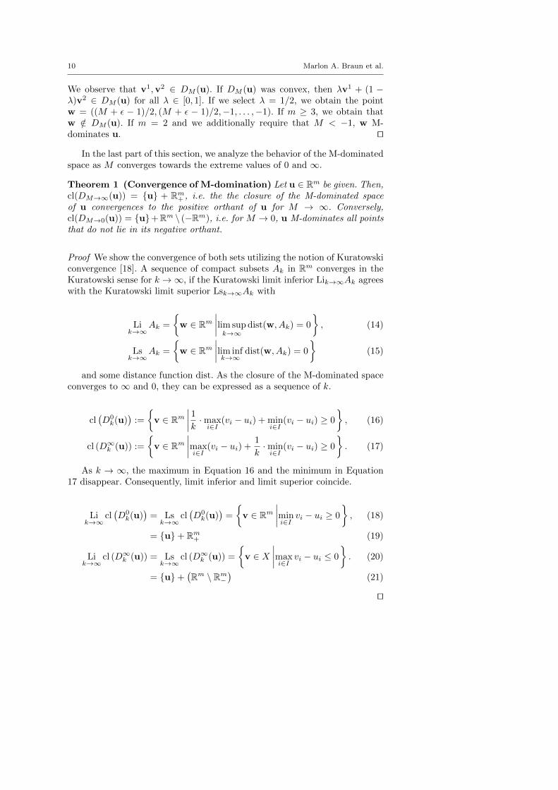
We observe that v1,v2 ∈ DM (u). If DM (u) was convex, then λv1 + (1 −λ)v2 ∈ DM (u) for all λ ∈ [0, 1]. If we select λ = 1/2, we obtain the pointw = ((M + ε − 1)/2, (M + ε − 1)/2,−1, . . . ,−1). If m ≥ 3, we obtain thatw /∈ DM (u). If m = 2 and we additionally require that M < −1, w M-dominates u. ut

In the last part of this section, we analyze the behavior of the M-dominatedspace as M converges towards the extreme values of 0 and ∞.

Theorem 1 (Convergence of M-domination) Let u ∈ Rm be given. Then,cl(DM→∞(u)) = u + Rm+ , i.e. the the closure of the M-dominated spaceof u convergences to the positive orthant of u for M → ∞. Conversely,cl(DM→0(u)) = u+Rm \ (−Rm), i.e. for M → 0, u M-dominates all pointsthat do not lie in its negative orthant.

Proof We show the convergence of both sets utilizing the notion of Kuratowskiconvergence [18]. A sequence of compact subsets Ak in Rm converges in theKuratowski sense for k →∞, if the Kuratowski limit inferior Lik→∞Ak agreeswith the Kuratowski limit superior Lsk→∞Ak with

Lik→∞

Ak =

w ∈ Rm

∣∣∣∣lim supk→∞

dist(w, Ak) = 0

, (14)

Lsk→∞

Ak =

w ∈ Rm

∣∣∣∣lim infk→∞

dist(w, Ak) = 0

(15)

and some distance function dist. As the closure of the M-dominated spaceconverges to ∞ and 0, they can be expressed as a sequence of k.

cl(D0k(u)

):=

v ∈ Rm

∣∣∣∣1k ·maxi∈I

(vi − ui) + mini∈I

(vi − ui) ≥ 0

, (16)

cl (D∞k (u)) :=

v ∈ Rm


(vi − ui) +1

k·mini∈I

(vi − ui) ≥ 0

. (17)

As k → ∞, the maximum in Equation 16 and the minimum in Equation17 disappear. Consequently, limit inferior and limit superior coincide.

Lik→∞

cl(D0k(u)

)= Lsk→∞

cl(D0k(u)

)=

v ∈ Rm

∣∣∣∣mini∈I

vi − ui ≥ 0

, (18)

= u+ Rm+ (19)

Lik→∞

cl (D∞k (u)) = Lsk→∞

cl (D∞k (u)) =

v ∈ X


vi − ui ≤ 0

. (20)

= u+(Rm \ Rm−

)(21)

ut


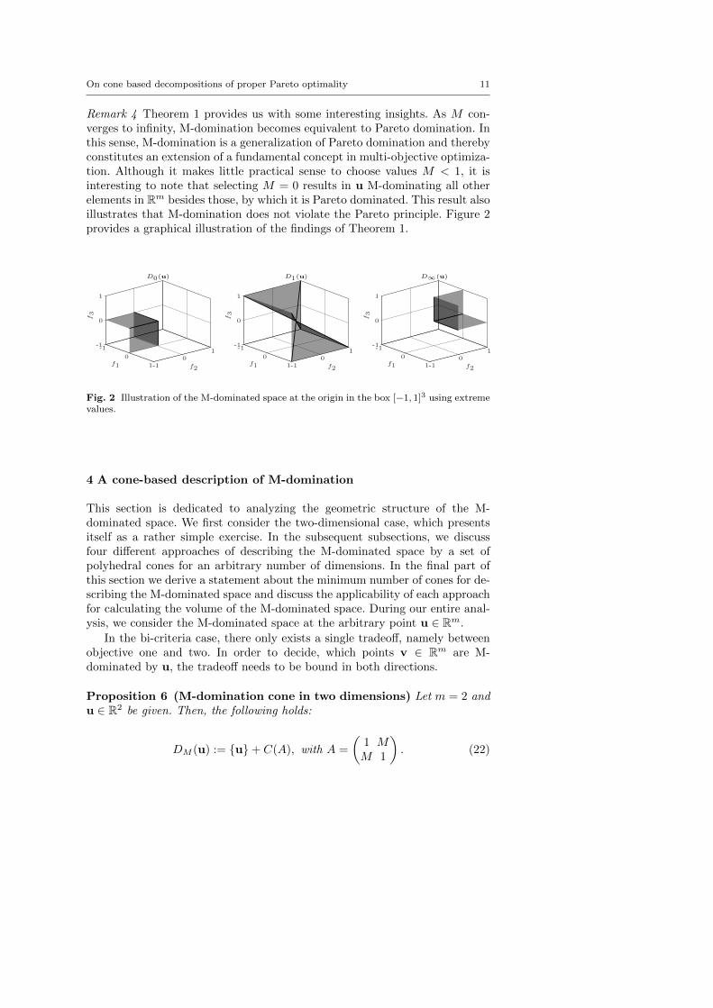
Remark 4 Theorem 1 provides us with some interesting insights. As M con-verges to infinity, M-domination becomes equivalent to Pareto domination. Inthis sense, M-domination is a generalization of Pareto domination and therebyconstitutes an extension of a fundamental concept in multi-objective optimiza-tion. Although it makes little practical sense to choose values M < 1, it isinteresting to note that selecting M = 0 results in u M-dominating all otherelements in Rm besides those, by which it is Pareto dominated. This result alsoillustrates that M-domination does not violate the Pareto principle. Figure 2provides a graphical illustration of the findings of Theorem 1.

f3

f2f1

D0(u)

-1

0

1-10

1-1

0

1

f3

f2f1

D1(u)

-1

0

1-10

1-1

0

1

f3

f2f1

D∞(u)

-1

0

1-10

1-1

0

1

Fig. 2 Illustration of the M-dominated space at the origin in the box [−1, 1]3 using extremevalues.

4 A cone-based description of M-domination

This section is dedicated to analyzing the geometric structure of the M-dominated space. We first consider the two-dimensional case, which presentsitself as a rather simple exercise. In the subsequent subsections, we discussfour different approaches of describing the M-dominated space by a set ofpolyhedral cones for an arbitrary number of dimensions. In the final part ofthis section we derive a statement about the minimum number of cones for de-scribing the M-dominated space and discuss the applicability of each approachfor calculating the volume of the M-dominated space. During our entire anal-ysis, we consider the M-dominated space at the arbitrary point u ∈ Rm.

In the bi-criteria case, there only exists a single tradeoff, namely betweenobjective one and two. In order to decide, which points v ∈ Rm are M-dominated by u, the tradeoff needs to be bound in both directions.

Proposition 6 (M-domination cone in two dimensions) Let m = 2 andu ∈ R2 be given. Then, the following holds:

DM (u) := u+ C(A), with A =

(1 MM 1

). (22)


Proof Let us first consider d1 > d2. In this case, u M v if d1+M ·d2 > 0. Thisis the same as (1,M)·(d1, d2)T > 0. If d1 < d2 we get that (M, 1)·(d1, d2)T > 0.Since the tradeoff must be bound in both directions, combining the two resultswe obtain the matrix A. ut

4.1 Ordered objectives approach

The situation presents itself in a more complex manner for three and moreobjectives. As an introductory example, let us assume we find ourselves inthree dimensions. If u1 > v1, the tradeoff of objective one may either bebound by objective two, three or even both at the same time. The challengelies in representing all these feasible cases in systems of linear inequalities. Inorder to structure our analysis, we consider the vector d = v − u. We canorder the elements in d from largest to smallest. Knowing the largest andsmallest difference, we can directly assess, whether the tradeoff from u to vis bounded by M . The order of the elements in d can be represented by aseries of linear inequalities. We provide an example in three dimensions. Table1 lists the necessary linear inequalities for the case where d1 ≥ d2 ≥ d3 and(23) yields the corresponding matrix.

Table 1 Example of the ordered objectives approach.

d1 ≥ d2 ≥ d3

d1 + M · d3 > 0d1 − d2 ≥ 0d2 − d3 ≥ 0

Ao123 =

1 0 M1 −1 00 1 −1

(23)

We acknowledge that the system in Table 1 does not exactly adhere to Def-inition 4, since the second and third inequality are not strict. This, however, isonly a minor nuisance. The cone described by the system in Table 1 is partiallyopen and closed. It is open towards the boundary of the M-dominated spaceand closed towards the interior of the M-dominated space. For quantifying theM-dominated space of u, it is irrelevant if the cone is open or closed as wemay always consider its closure.

The example we have discussed covers only one feasible ordering. Thereexist six different permutations for three elements, so there are six cases toconsider. Each case can be translated to a matrix that in turn representsa polyhedral cone. The union of these cones constitutes the M-dominatedspace of u. We therefore denote this notion by ordered objectives approach.

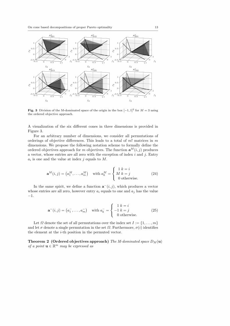
On cone based decompositions of proper Pareto optimality 13f3

f2

f1

Ao321

-1

0

1-0.5 0 0.5 1

-0.5

0

0.5

1

f3

f2

f1

Ao312

-1

0

1-0.5 0 0.5 1

-0.5

0

0.5

1

f3

f2

f1

Ao231

-1

0

1-0.5 0 0.5 1

-0.5

0

0.5

1

f3

f2

f1

Ao213

-1

0

1-0.5 0 0.5 1

-0.5

0

0.5

1

f3

f2

f1

Ao123

-1

0

1-0.5 0 0.5 1

-0.5

0

0.5

1

f3

f2

f1

Ao132

-1

0

1-0.5 0 0.5 1

-0.5

0

0.5

1

Fig. 3 Division of the M-dominated space of the origin in the box [−1, 1]3 for M = 3 usingthe ordered objective approach.

A visualization of the six different cones in three dimensions is provided inFigure 3.

For an arbitrary number of dimensions, we consider all permutations oforderings of objective differences. This leads to a total of m! matrices in mdimensions. We propose the following notation scheme to formally define theordered objectives approach for m objectives. The function aM (i, j) producesa vector, whose entries are all zero with the exception of index i and j. Entryai is one and the value at index j equals to M .

aM (i, j) =(aM1 , . . . , a

Mm

)with aMk =

1 k = iM k = j

0 otherwise.(24)

In the same spirit, we define a function a−(i, j), which produces a vectorwhose entries are all zero, however entry ai equals to one and aj has the value−1.

a−(i, j) =(a−1 , . . . , a

−m

)with a−k =

1 k = i−1 k = j

0 otherwise.(25)

Let Ω denote the set of all permutations over the index set I := 1, . . . ,mand let σ denote a single permutation in the set Ω. Furthermore, σ(i) identifiesthe element at the i-th position in the permuted vector.

Theorem 2 (Ordered objectives approach) The M-dominated space DM (u)of a point u ∈ Rm may be expressed as


DM (u) = u+⋃σ∈Ω

C(Aoσ) (26)

with

Aoσ =

aM (σ(1), σ(m))1×m

a−(σ(1), σ(2))1×m

a−(σ(2), σ(3))1×m

...a−(σ(m− 1), σ(m))1×m

. (27)

Proof Let Aσ denote the matrix that represents the system of linear inequali-ties induced by the permutation σ.2 We know that

⋃σ∈Ω C(Aσ) = Rm. C(Aoσ)

contains exactly those elements of C(Aσ) that are M-dominated by u. We con-clude that the union of all C(Aoσ) is equivalent to the non-dominated space.

ut

4.2 Min/max ordered objectives approach

The ordered objective approach serves well as a conceptual illustration, how-ever proves to be impractical for volume calculation in higher dimensions, sincethe number of matrices used for describing the M-dominated space grows fac-torially. A closer analysis of the ordered objectives approach, however, revealsa possibility for reducing the number of matrices required. The exact order ofthe entries in d is irrelevant for checking for M-domination. Instead, it is de-cisive that the maximum and minimum of d are known, in order to determineif (8) holds. The other objectives are exclusively required to lie between theminimum and the maximum element of d.

Let us assume that i is the index of the maximum element in d and j theindex of its minimum element. In order to formally represent the system oflinear inequalities that ensures that all other entries in d lie between dj anddi, we propose the following notation scheme. The function B+(i, j) generatesa matrix that represents the system of linear inequalities, which states thatdi is larger than all other values in d with the exception of dj . This matrixis a combination of the negative identity matrix −Im−2, a column vector ofones 1m−2 and a column vector of zeros 0m−2. The resulting matrix B+(i, j)is of size m − 2 ×m. B+(i, j) is generated by inserting 1m−2 and 0m−2 into−Im−2, such that both vectors are located at the column indexes i and j inthe resulting matrix B+(i, j). A formal summary is given in (28):

2 Aσ is equivalent to Aoσ with the exception of the first row, which states the M-dominationcondition.


B+(i, j) with b+kl =

1 k = i

−1

(k = l) ∧ (k < i, j)(k = l − 1) ∧ ((k > i)⊗ (k > j))(k = l − 2) ∧ (k > i, j)

0 otherwise,

(28)

where ⊗ describes the XOR operator. Conversely, a matrix for expressingthe system of linear inequalities stating that all elements in d are greater thandj with the exception of di may be described correspondingly. We denote thismatrix by B−(i, j). B−(i, j) is generated by inserting 0m−2 and a vector ofnegative ones −1m−2 into the positive identity matrix Im−2, such that 0m−2resides at index i and −1m−2 at index j in the result matrix.

B−(i, j) with b−kl =

−1 k = j

1

(k = l) ∧ (k < i, j)(k = l − 1) ∧ ((k > i)⊗ (k > j))(k = l − 2) ∧ (k > i, j)

0 otherwise.

(29)

The definition of B+(i, j) and B−(i, j) allows us to formally define themin/max ordered objectives approach.

Theorem 3 (Min/max ordered objectives approach) The M-dominatedspace DM (u) of a point u ∈ Rm may be expressed as

DM (u) = u+⋃i∈I

⋃j∈I\i

C(Asij) (30)

with

Ammij =

aM (i, j)1×mB+(i, j)m−2×mB−(i, j)m−2×m

. (31)

Proof Let Aij denote the matrix describing the linear system, for which di isthe maximum and dj the minimum direction while all other elements of d arebound between those two directions.3 We know that

⋃i∈I⋃j∈I\iAij = Rm.

Consequently, C(Ammij ) contains all elements of C(Aij) that are M-dominatedby u. We conclude that the union of all C(Ammij ) is equivalent to the M-dominated space by u. ut

3 Aij is equivalent to Asij with the exception of the first row, which states the M-domination condition.


In order to illustrate the min/max ordered objectives approach, let usconsider the matrix Amm21 for m = 4:

As21 =

M 1 0 00 1 −1 00 1 0 −1−1 0 1 0−1 0 0 1

. (32)

The min/max ordered objectives approach increases the number of linearinequalities required for describing a single order from m− 1 to 2m− 2. Thisin turn implies that the number of matrix rows is increased from m to 2m−3.However, this disadvantage is counteracted by reducing the number of totalcones. Since we only consider the largest and smallest difference, we deal witha 2-permutation of m objectives, which is equal to P (m, 2) = m(m− 1).

4.3 Maximum element approach

The next approach we present further relaxes the prerequisite of having aparticular order of objectives for checking the M-domination condition. Letus therefore first consider the case in three dimensions, where the objectivedifferences are ordered according to their magnitude in the following way:d1 ≥ d2 ≥ d3. We know that u M v if d1 + M · d3 > 0. If this inequalityholds, we automatically obtain by transitivity that d1 +M · d2 > 0 is true aswell. We conclude that the exact order of objective differences is irrelevant, aslong as we can assert that d1 is the largest element in d and the tradeoff of allother objectives is bound to d1.

In order to simplify the notation of the maximum ordered objectives ap-proach, we propose the following functions. B+(i) represents the matrix de-scribing the system of linear inequalities stating that all other elements in dare smaller than di. The function is generated by inserting the column vectorof ones 1m−1 in the negative indentity matrix −Im−1 at index i. A formaldefinition is provided in (33).

B+(i) with b+kl =

1 k = i

−1

(k = l) ∧ (k < i)(k = l − 1) ∧ (k > i)

0 otherwise.

(33)

The function BM (i) is created by inserting column vector 1m−1 at positioni in the product of the identity matrix Im−1 by M . This matrix states therequirement for all objectives being bound by objective i:

BM (i) with b+kl =

1 k = i

M

(k = l) ∧ (k < i)(k = l − 1) ∧ (k > i)

0 otherwise.

(34)


Theorem 4 (Maximum element approach) The M-dominated space DM (u)of a point u ∈ Rm may be expressed as

DM (u) = u+⋃i∈I

C(Amaxi ) (35)

with

Amaxi =

(BM (i)m−1×mB+(i)m−1×m

). (36)

Proof We know that⋃i∈I C(BM (i)) = Rm. C(Amaxi ) contains exactly those

points of C(BM (i)) that are M-dominated by u. We conclude that DM (u) =⋃i∈I C(Amaxi ). ut

The maximum element approach requires only m cones for describing theM-dominated space. Establishing that di is the largest element of d needs minequalities. Bounding the tradeoff of all goals to objective j takes the samenumber of inequalities. This results in 2m− 2 rows per matrix.

4.4 Minimum matrix approach

The minimum matrix approach is a subsequent relaxation of the maximumelement approach. The maximum element approach explicitly states by im-plementing the block matrix B+(i) that di is the largest element in d. Thisrequirement can also be met by bounding the tradeoff of objective i to anyother objective j ∈ I \ i.

Theorem 5 (Minimum matrix approach) The M-dominated space DM (u)of a point u ∈ Rm may be expressed as

DM (u) = u+⋃i∈I

C(Amini ) (37)

with

Amini =

(BM (i)m−1×m

aM ((i mod m) + 1, i)1×m

). (38)

Proof It is sufficient to show that C(Amaxi ) ⊆ C(Amini ) and that C(Amini ) onlyincludes M-dominated elements. If di = arg maxj∈I dj , then Mdi + dk > 0 fork ∈ I, if B+(i)j > 0. This implies that C(Amaxi ) is a subset of C(Amini ).If di is not the maximum element of d, then Mdi + dk > 0 only holds ifarg maxj∈I(dj) +M arg minj∈I(dj) > 0, which is equivalent to u M v. ut


The minimum matrix approach requires only m matrices each having mrows. The linear inequalities of the underlying system translate directly tothe matrix as of Definition 4, since they are all strict in comparison to theother approaches. Still, the minimum matrix approach features one distinctdisadvantage. The cones C(Amini ) are overlapping. This is because a singletradeoff may be bound by multiple objectives. The issue is illustrated in Figure4, which shows the different partitions of the minimum matrix approach forM = 3. The issue of overlapping partitions is discussed in the next subsection.

f3

f2

f1

Amin1

-1

0

1-0.5 0 0.5 1

-0.5

0

0.5

1

f3

f2

f1

Amin2

-1

0

1-0.5 0 0.5 1

-0.5

0

0.5

1

f3

f2

f1

Amin3

-1

0

1-0.5 0 0.5 1

-0.5

0

0.5

1

Fig. 4 Division of the M-dominated space of the origin in [−1, 1]3 for M = 3 using theminimum matrix approach.

4.5 Minimum number of cones and summary

One might wonder if it possible to even further reduce the number of poly-hedral cones for describing the M-dominated space. Theorem 6 shows that mserves as lower bound for the number of convex cones in m dimensions.

Theorem 6 Describing the M-dominated space DM (u) of a point u ∈ Rm bya union of convex cones requires at least m cones for m > 2.

Proof Without loss of generality let us consider the M-dominated space of theorigin u = (0, . . . , 0) and let an arbitrary but fixed M be given. Let us considerthe point vi with i ∈ I, whose entries are all −1 with the exception of entryi, which equals M + ε with ε ∈ (0,M ]. From the proof of Proposition 5 weobtain that v1 and v2 cannot lie in the same convex partition of DM (u). Thisresult holds for any vj and vk with j, k ∈ I, j 6= k. Since |I| = m, we requireat least m convex partitions of DM (u).

ut

The four different approaches we have presented in the previous subsec-tions can all be utilized to calculate the volume of the M-dominated space withrespect to a given reference point r. Computing the volume of u with respectto the partition matrix A and r is done in the following way. We calculate thevolume of the orthotope defined by the vertices A ·u and A · r. The orthotope


volume is then divided by the determinant of A if the matrix is square or theroot of det(ATA) if A is rectangular to obtain the partition volume of u accord-ing to A and r. Summing up all partition volumes yields the overall volumeof the M-dominated space with respect to r. Using the transformation schemepresented in the previous paragraph allows us to reuse existing hypervolumecalculation techniques [3,29] based on the Pareto domination principle.

Calculating the joint hypervolume of a set of solutions is a non-trivial task,as individual domination cones are usually overlapping. The runtime of state-of-the-art methods increases exponentially in the number of objectives. Wehave therefore identified three criteria that determine the effectiveness of thepartitioning approaches presented in this work. The total number of conesdetermines how many translations and single volume calculations need to beconducted. The matrix size of each cone decideds upon the complexity of thevolume calculation, as the number of rows determines the dimensionality ofthe transformed coordinate system. The number of columns is identical forall approaches and has the value m. Finally, overlapping cones prohibit thecomputation of the exact volume, as overlapping subvolumes are includedmultiple times.

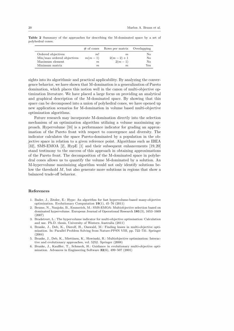
Table 2 summarizes our findings with respect to these three performancecriteria. The number of cones grows factorially in the ordered objectives ap-proach, which makes it only suitable for application in lower dimensions. How-ever, it is the only approach that retains the dimensionality of the originalcoordinate system that is non-overlapping. The min/max ordered objectivesapproach requires only a quadratic number of cones, however the dimension-ality of the transformed coordination system increases almost by a factor oftwo in comparison. The maximum element approach, in comparison, requiresjust m cones and needs only one additional matrix row. Although both ap-proaches are non-dominated to each other, we can argue that trading in onematrix row for practically squaring the number of matrices represents an un-acceptable tradeoff. The minimum matrix approach features the minimumnumber of cones and rows per matrix, however the cones it describes are over-lapping. This property does not necessarily imply that the minimum matrixapproach is ill-suited for finding volume-maximizing distributions. We conjec-ture, however, that an algorithmic application could lead to an overly strongcrowding of solutions in certain regions that does not concur with the notionof M-domination. We observe that no approach is optimal in each criterion.However, for an algorithmic application we suggest further investigating eitherthe maximum element or minimum matrix approach, as they appear to be theonly viable options in higher dimensions.

5 Conclusion

In this paper, we have shown how the notion of proper Pareto optimality maybe translated to the dominance relation M-domination. We have thoroughlydiscussed the mathematical properties of M-domination yielding important in-


Table 2 Summary of the approaches for describing the M-dominated space by a set ofpolyhedral cones.

# of cones Rows per matrix Overlapping

Ordered objectives m! m NoMin/max ordered objectives m(m− 1) 2(m− 2) + 1 NoMaximum element m 2(m− 1) NoMinimum matrix m m Yes

sights into its algorithmic and practical applicability. By analyzing the conver-gence behavior, we have shown that M-domination is a generalization of Paretodomination, which places this notion well in the canon of multi-objective op-timization literature. We have placed a large focus on providing an analyticaland graphical description of the M-dominated space. By showing that thisspace can be decomposed into a union of polyhedral cones, we have opened upnew application scenarios for M-domination in volume based multi-objectiveoptimization algorithms.

Future research may incorporate M-domination directly into the selectionmechanism of an optimization algorithm utilizing a volume maximizing ap-proach. Hypervolume [34] is a performance indicator for grading an approx-imation of the Pareto front with respect to convergence and diversity. Theindicator calculates the space Pareto-dominated by a population in the ob-jective space in relation to a given reference point. Algorithms such as IBEA[32], SMS-EMOA [2], HypE [1] and their subsequent enhancements [19,20]stand testimony to the success of this approach in obtaining approximationsof the Pareto front. The decomposition of the M-dominated space in polyhe-dral cones allows us to quantify the volume M-dominated by a solution. AnM-hypervolume maximizing algorithm would not only identify solutions be-low the threshold M , but also generate more solutions in regions that show abalanced trade-off behavior.

References

1. Bader, J., Zitzler, E.: Hype: An algorithm for fast hypervolume-based many-objectiveoptimization. Evolutionary Computation 19(1), 45–76 (2011)

2. Beume, N., Naujoks, B., Emmerich, M.: SMS-EMOA: Multiobjective selection based ondominated hypervolume. European Journal of Operational Research 181(3), 1653–1669(2007)

3. Bradstreet, L.: The hypervolume indicator for multi-objective optimisation: Calculationand use. Ph.D. thesis, University of Western Australia (2011)

4. Branke, J., Deb, K., Dierolf, H., Osswald, M.: Finding knees in multi-objective opti-mization. In: Parallel Problem Solving from Nature-PPSN VIII, pp. 722–731. Springer(2004)

5. Branke, J., Deb, K., Miettinen, K., Slowinski, R.: Multiobjective optimization: Interac-tive and evolutionary approaches, vol. 5252. Springer (2008)

6. Branke, J., Kaußler, T., Schmeck, H.: Guidance in evolutionary multi-objective opti-mization. Advances in Engineering Software 32(6), 499–507 (2001)


7. Braun, M.A., Shukla, P.K., Schmeck, H.: Preference ranking schemes in multi-objectiveevolutionary algorithms. In: Evolutionary Multi-Criterion Optimization, pp. 226–240.Springer (2011)

8. Coello, C.C., Lamont, G.B., Van Veldhuizen, D.A.: Evolutionary algorithms for solvingmulti-objective problems. Springer (2007)

9. Deb, K.: Multi-objective optimization using evolutionary algorithms, vol. 16. JohnWiley & Sons (2001)

10. Deb, K., Gupta, S.: Understanding knee points in bicriteria problems and their impli-cations as preferred solution principles. Engineering optimization 43(11), 1175–1204(2011)

11. Deb, K., Jain, H.: An evolutionary many-objective optimization algorithm usingreference-point based non-dominated sorting approach, part I: Solving problems withbox constraints. Evolutionary Computation (2013)

12. Deb, K., Pratap, A., Agarwal, S., Meyarivan, T.: A fast and elitist multiobjective geneticalgorithm: NSGA-II. Evolutionary Computation, IEEE Transactions on 6(2), 182–197(2002)

13. Deb, K., Srinivasan, A.: Innovization: Innovating design principles through optimization.In: Proceedings of the 8th annual conference on Genetic and evolutionary computation,pp. 1629–1636. ACM (2006)

14. Ehrgott, M.: Multicriteria optimization, vol. 2. Springer (2005)15. Geoffrion, A.M.: Proper efficiency and the theory of vector maximization. Journal of

Mathematical Analysis and Applications 22, 618–630 (1968)16. Hirsch, C., Shukla, P.K., Schmeck, H.: Variable preference modeling using multi-

objective evolutionary algorithms. In: Evolutionary Multi-Criterion Optimization, pp.91–105. Springer (2011)

17. Hunt, B.J.: Multiobjective programming with convex cones: Methodology and applica-tions. Ph.D. thesis, Clemson University (2004)

18. Kuratowski, K.: Topology. Vol. I. New edition, revised and augmented. Translatedfrom the French by J. Jaworowski. Academic Press, New York-London; PanstwoweWydawnictwo Naukowe, Warsaw (1966)

19. Menchaca-Mendez, A., Coello Coello, C.: A new selection mechanism based on hyper-volume and its locality property. In: Evolutionary Computation (CEC), 2013 IEEECongress on, pp. 924–931. IEEE (2013)

20. Menchaca-Mendez, A., Montero, E., Riff, M.C., Coello, C.A.C.: A more efficient selec-tion scheme in isms-emoa. In: Advances in Artificial Intelligence–IBERAMIA 2014, pp.371–380. Springer (2014)

21. Miettinen, K.: Nonlinear multiobjective optimization, vol. 12. Springer (1999)22. Pareto, V.: Cours d’economie politique. Librairie Droz (1896)23. Shukla, P.K.: In search of proper pareto-optimal solutions using multi-objective evo-

lutionary algorithms. In: Computational Science–ICCS 2007, pp. 1013–1020. Springer(2007)

24. Shukla, P.K., Braun, M.A.: Indicator based search in variable orderings: theory andalgorithms. In: Evolutionary Multi-Criterion Optimization, pp. 66–80. Springer BerlinHeidelberg (2013)

25. Shukla, P.K., Braun, M.A., Schmeck, H.: Theory and algorithms for finding knees. In:Evolutionary Multi-Criterion Optimization, pp. 156–170. Springer Berlin Heidelberg(2013)

26. Shukla, P.K., Cipold, M.P., Bachmann, C., Schmeck, H.: On homogenization of coalin longitudinal blending beds. In: Proceedings of the 2014 conference on Genetic andevolutionary computation, pp. 1199–1206. ACM (2014)

27. Shukla, P.K., Hirsch, C., Schmeck, H.: A framework for incorporating trade-off informa-tion using multi-objective evolutionary algorithms. In: Parallel Problem Solving fromNature, PPSN XI, pp. 131–140. Springer (2010)

28. Somers, D.M.: Design and experimental results for a natural-laminar-flow airfoil forgeneral aviation applications. Tech. rep., NASA (1981)

29. While, L., Bradstreet, L.: Applying the wfg algorithm to calculate incremental hyper-volumes. In: Evolutionary Computation (CEC), 2012 IEEE Congress on, pp. 1–8. IEEE(2012)


30. Wiecek, M.M.: Advances in cone-based preference modeling for decision making withmultiple criteria. Decision Making in Manufacturing and Services 1(1-2), 153–173 (2007)

31. Zhang, Q., Li, H.: MOEA/D: A multiobjective evolutionary algorithm based on decom-position. Evolutionary Computation, IEEE Transactions on 11(6), 712 –731 (2007).DOI 10.1109/TEVC.2007.892759

32. Zitzler, E., Kunzli, S.: Indicator-based selection in multiobjective search. In: ParallelProblem Solving from Nature-PPSN VIII, pp. 832–842. Springer (2004)

33. Zitzler, E., Laumanns, M., Thiele, L.: SPEA2: Improving the strength Pareto evolu-tionary algorithm. Tech. Rep. 103, Computer Engineering and Networks Laboratory(TIK), Swiss Federal Institute of Technology (ETH), Zurich, Switzerland (2001)

34. Zitzler, E., Thiele, L.: Multiobjective evolutionary algorithms: a comparative case studyand the strength pareto approach. Evolutionary Computation, IEEE Transactions on3(4), 257–271 (1999)

On cone based decompositions of proper Pareto optimality · On cone based decompositions of proper...

Documents

Transcript of On cone based decompositions of proper Pareto optimality · On cone based decompositions of proper...