2. Pareto optimality and the Pareto criterion...principle and the concept of Pareto optimality. This...

2. Pareto optimality and the Pareto criterion

Determination of economic criteria for public policy evaluation has been a subject ofgreat debate. The difficulty stems from the inability to decide on purely economic groundshow the goods and services produced in an economy should be distributed among indi-viduals. Issues of distribution and equity are political and moral as well as economic innature.

Classical economists such as Bentham (1961, first published 1823) long ago developedthe concept of a social welfare function to measure the welfare of society as a function ofthe utilities of all individuals. The objective was to establish a complete social ordering ofall possible alternative states of the world. A social ordering, in principle, permits com-parison and choice among alternative states and would allow economists to determineprecisely which set of policies maximize the good of society. The problem is that agree-ment on the form of a social welfare function cannot be reached so the use of such aconcept has been clouded with controversy. Many functional forms have been proposedand defended on moral, ethical and philosophical grounds with specific considerationsgiven to equity, liberty and justice (see Sections 3.3 and 3.4 for more details). Because ofthe subjectivity of these arguments, agreement is unlikely ever to be reached. Even ifagreement were reached among economists, policy-makers may be unwilling to acceptsuch judgments by economists as the basis for public policy choice.

Because use of a social welfare function is clouded by controversy, many economistshave tried to maintain objectivity and the claim of their professional practice as a scienceby avoiding value judgments. A value judgment is simply a subjective statement aboutwhat is of value to society that helps to determine the social ordering of alternative statesof the world. It is subjective in the sense that it cannot be totally supported by evidence.It is not a judgment of fact. The attempt to avoid value judgments led to development ofthe Pareto principle.

The Pareto criterion was introduced in the nineteenth century by the eminent Italianeconomist, Vilfredo Pareto (1896). Its potential for application to public policy choices,however, is still very much discussed. By this criterion, a policy change is socially desir-able if, by the change, everyone can be made better off, or at least some are made betteroff, while no one is made worse off. If there are any who lose, the criterion is not met. Inhis book The Zero-Sum Society: Distribution and the Possibilities for Economic Change,Lester Thurow (1980) contends that many good projects do not get under way simplybecause project managers are unwilling to pay compensation to those who would actuallybe made worse off. If this is correct, perhaps policy measures should be considered thatmeet the Pareto criterion. That is, perhaps policy measures that include the payment ofcompensation, so that everyone is made better off, should be considered. For example,those who support tariffs argue that their removal results in short-term loss of jobs forwhich workers are not adequately compensated. Trade theory shows that there are eco-nomic gains from free trade, but the distribution of these gains is what the workers object

14

to. This objection would probably not arise if only policies that met the Pareto criterionwere considered. However, as will become clear, there are also limitations to using thePareto criterion to rank policy choices.

A large part of theoretical welfare economics and its application is based on the Paretoprinciple and the concept of Pareto optimality. This chapter discusses both Pareto opti-mality and the Pareto criterion in a general equilibrium setting. The consideration ofthese concepts in a general equilibrium context enables greater understanding of theassumptions, limitations and generalizations associated with applying welfare economicsto real-world problems discussed in later chapters.

2.1 PARETO OPTIMALITY AND THE PARETO CRITERIONDEFINED

The Pareto criterion is a technique for comparing or ranking alternative states of theeconomy. By this criterion, if it is possible to make at least one person better off whenmoving from state A to state B without making anyone else worse off, state B is rankedhigher by society than state A. If this is the case, a movement from state A to state B rep-resents a Pareto improvement, or state B is Pareto superior to state A. As an example,suppose a new technology is introduced that causes lower food prices and, at the sametime, does not harm anyone by (for example) causing unemployment or reduced profits.The introduction of such a technology would be a Pareto improvement.

To say that society should make movements that are Pareto improvements is, of course,a value judgment but one that enjoys widespread acceptance. Some would disagree,however, if policies continuously make the rich richer while the poor remain unaffected.

If society finds itself in a position from which there is no feasible Pareto improvement,such a state is called a Pareto optimum. That is, a Pareto-optimal state is defined as a statefrom which it is impossible to make one person better off without making another personworse off. It is important to stress that, even though a Pareto-optimal state is reached, thisin no way implies that society is equitable in terms of income distribution. For example,as will become evident later, a Pareto-optimum position is consistent with a state of natureeven where the distribution of income is highly skewed.

If the economy is not at a Pareto optimum, there is some inefficiency in the system.When output is divisible, it is always theoretically possible to make everyone better off inmoving from a Pareto-inferior position to a Pareto-superior position. Hence, Pareto-optimal states are also referred to as Pareto-efficient states, and the Pareto criterion isreferred to as an efficiency criterion. Efficiency in this context is associated with getting asmuch as possible for society from its limited resources. Note, however, that the Pareto cri-terion can be used to compare two inefficient states as well. That is, one inefficient statemay represent a Pareto improvement over another inefficient state.

Of course, it may be politically infeasible to move from certain inefficient states tocertain Pareto-superior states. If Thurow is correct, the only feasible options may bemoves to positions where at least one person is made worse off. States where one personis made better off and another is made worse off are referred to as Pareto-noncomparablestates. Note that all of these Pareto-related concepts are defined independently of soci-eties’ institutional arrangements for production, marketing and trade.

Pareto optimality and the Pareto criterion 15

2.2 THE PURE CONSUMPTION CASE

Now consider the concepts of Pareto optimality and the Pareto criterion for the pureexchange case, that is, the optimal allocation of goods among individuals where the goodsare, in fact, already produced. In this context, a set of marginal exchange conditions charac-terizing Pareto-efficient states can be developed. Suppose that there are two individuals, Aand B, and quantities of two goods, q1 and q2, which have been produced and can be distrib-uted between the two individuals. This situation is represented by the Edgeworth–Bowleybox in Figure 2.1, where the width of the box measures the total amount of q1 producedand the height of the box measures the total amount of q2 produced.

The indifference map for individual A is displayed in the box in standard form with OAas the origin. Three indifference curves for individual A – labeled U1

A, U2A, and U3

A – aredrawn in the box. The indifference map for individual B with indifference curves U1

B andU2

B has OB as the origin and thus appears upside down and reversed. Displaying theindifference maps of individuals A and B in this manner ensures that every point in thebox represents a particular distribution of q1 and q2 or a state of the economy in the pureexchange case. For example, at point a, individual A is endowed with q1

1 of good q1 andq2

1 of good q2, while the remainder of each, q1!q11andq2 !q2

1, respectively, is distributedto individual B.

The solid line in Figure 2.1 running from OA to OB through points a and b is known asthe contract curve and is constructed by connecting all points of tangency betweenindifference curves for individuals A and B. At all points on this line, both consumers’indifference curves have the same slope or, in other words, both consumers have equalmarginal rates of substitution for goods q1 and q2. The marginal rate of substitution meas-ures the rate at which a consumer is willing to trade one good for another at the margin.

16 The welfare economics of public policy

Figure 2.1

Goo

d q 2

{U1A

U2A

∆q1

q12q1

1 q1

U3A

U1B

e

c

d

b

f

a

U2B

OA

q21

q22

q2

Good q1

OB

The marginal rate of substitution for each consumer generally varies along the contractcurve for both consumers. The slope of the indifference curves at point a, for example, isnot necessarily the same as the slope at point b.

Now, consider the possibility of using the Pareto criterion to compare or rank alterna-tive states of the economy. For example, compare point c with other points in theEdgeworth-Bowley box. First, compare point c with points inside the lightly shaded area.At point c, the marginal rate of substitution of q1 for q2 for individual A, denoted byMRSA

q1q2is greater than the marginal rate of substitution of q1 for q2 for individual B,

denoted by MRSBq1q2

. This implies that the amount of q2 that individual A is willing to giveup to obtain an additional unit of q1 exceeds the amount individual B is willing to acceptto give up a unit of q1. For the marginal increment !q1 in Figure 2.1, this excess corre-sponds to the distance de. That is, individual A is willing to pay df of q2 to obtain !q1,whereas individual B requires only ef of q2 to give up !q1. If this excess of willingness-to-pay over willingness-to-accept is not paid to individual B, and individual B is paid onlythe minimum amount necessary, then point e is Pareto superior to point c because indi-vidual A is made better off and individual B is no worse off. If the excess is paid to indi-vidual B, the movement is to point d, which is again Pareto superior to point c becauseindividual B is made better off and individual A is no worse off. If any nontrivial portionof the excess is paid to individual B, both are made better off. Thus, all points, includingend points, on the line de are Pareto superior to point c. Similar reasoning suggests thata movement from point c to any point in the lightly shaded area can be shown to be animprovement on the basis of the Pareto criterion. Thus, all points in the lightly shadedarea are Pareto superior to point c.

Now consider comparison of point c with any point in the heavily shaded areas. Allpoints in the heavily shaded areas in Figure 2.1 are on indifference curves that are lowerfor both individuals A and B. Hence, points in the heavily shaded regions are Pareto infe-rior to point c because at least one individual is worse off and neither individual is betteroff.

Finally, consider comparison of point c with all remaining points that are not in shadedareas in the Edgeworth–Bowley box to discover a major shortcoming of the Pareto cri-terion: at all these points, one person is made better off and the other person is worse offrelative to point c. That is, at point a, individual B is better off than at point c but individ-ual A is worse off. Hence, these points are noncomparable using the Pareto principle.Improvements for society using the Pareto criterion can be identified only for cases whereeveryone gains or at least no one loses.

Now suppose that society starts at point c and moves to point e, making a Paretoimprovement. At point e, MRSA

q1q2"MRSB

q1q2and, hence, further gains from trade are

possible. Suppose that individuals A and B continue trading, with individual A giving upeach time the minimum amount of q2 necessary to obtain additional units of q1. In thismanner, the trade point moves along the indifference curve U1

B until point b is reached. Atpoint b, the amount of q2 that individual A is willing to give up to obtain an additionalunit of q1 is just equal to the amount of q2 that individual B would demand to give up aunit of q1. With any further movement, individual A would not be willing to pay the pricethat individual B would demand. In fact, a movement in any direction from point b mustmake at least one person worse off. Thus, point b is a Pareto optimum.

In this manner, one can verify that the marginal condition that holds at point b,


MRSAq1q2

!MRSBq1q2

, (2.1)

holds at all points on the contract curve. Thus, in the pure exchange case, any point on thecontract curve is a Pareto optimum. Pareto optimality implies that the marginal rate of sub-stitution between any two goods is the same for all consumers. The intuition of this condi-tion is clear because improvements for both individuals are possible (and Paretooptimality does not hold) if one individual is willing to give up more of one good to getone unit of another good than another individual is willing to accept to give up the oneunit.

2.3 PRODUCTION EFFICIENCY

Efficiency in production must also be considered when discussing Pareto optimality.Consider once again Figure 2.1 – but now assume that more of good q1, good q2, or bothcan be made available by improving the efficiency with which inputs are used. This wouldimply that individual B’s origin OB could be moved rightward, upward, or both. In any ofthese cases, any two indifference curves that were previously tangent on the contract curvewould now be separated by a region such as the lens-shaped, lightly shaded region inFigure 2.1. Thus, individual A, individual B, or both could be made better off. If produc-tion possibilities are considered and more of q1, q2, or both can be produced, then thepoints on the contract curve in Figure 2.1 will no longer be Pareto-optimal points. Statedconversely, where alternative production possibilities exist, the points on the contractcurve OAOB can be Pareto efficient only if the point (q1, q2) is an efficient output bundle.A Pareto-efficient output bundle is one in which more of one good cannot be producedwithout producing less of another.

However, an output point can be efficient only if inputs are allocated to their mostefficient uses. To see this, consider the production-efficiency frontier in the Edgeworth–Bowley box in Figure 2.2. This box is constructed by drawing the isoquant map for outputq1 as usual with isoquants q1

1, q12, and q1

3, but with the isoquant map for q2 upside downand reversed with origin at Oq

2. The total amounts of inputs x1 and x2 available are given

by x1 and x2. Any point in this box represents an allocation of inputs to the two produc-tion processes. For example, at point g, x1

1 of x1 and x21 of x2 are allocated to the produc-

tion of q1. The remainder of inputs x1"x11 and x2"x2

1 are allocated to the production ofq2.

Point g does not represent an efficient allocation of inputs because at point g the rateof technical substitution of x1 for x2 in the production of q1, denoted by RTSq2x1x2, is greaterthan the rate of technical substitution of x1 for x2 in the production of q2, denoted byRTSq1x1x2. The rate of technical substitution measures the rate at which one input can besubstituted for another while maintaining the same level of output. Thus, if an incrementof x1, say #x1, is shifted from the production of q2 to q1, then an increment of x2, say #x2,could be shifted to the production of q2 without decreasing the output of q1 from q1

1. Butonly an increment of ab$#x2 of x2 is necessary to maintain the output of q2 at the orig-inal level q2

1. This results from the fact that the marginal rate at which x1 substitutes for x2in q2 is less than the rate at which it substitutes for x2 in the production of q1. If, in theexchange of #x1 for an increment of x2, the output of q2 is kept constant at q2

1, the output


of q1 can be increased to q12. Thus, point g is an inefficient point. The output of q2 can be

increased without decreasing the output of q1. Clearly, if any amount of x2 on the segmentbc is allocated to q2 as !x1 is allocated to q1, the outputs of both q1 and q2 are increased.

By identical reasoning, point b can be established as an inefficient point. The output ofq1 can again be increased, holding q2 constant, by reallocating x1 to q1 and x2 to q2. Thisprocess can be continued until a state such as point d is reached. At point d, the amountof x2 that can be given up in exchange for an increment of x1, keeping q1 constant at q1

3,is precisely equal to the amount of x2 needed to keep q2 constant at q2

1 if an increment ofx1 is removed from the production of q2. It is impossible to increase the output of q1without decreasing the output of q2. Point d is thus a Pareto-efficient output point. But itis not unique. For example, point e, a point of tangency between q1

1 and q22, is also a

Pareto-efficient output point, as is point f. In fact, all points on the efficiency locus Oq1Oq2

are Pareto-efficient output points.Tangency of the isoquants in Figure 2.2 implies that

RTSq1x1x2"RTSq2x1x2

. (2.2)

Thus, to the earlier exchange conditions, this second set of conditions for Pareto optimal-ity can now be added. That is, Pareto optimality in production implies that the rate of tech-nical substitution between any two inputs is the same for all industries that use both inputs.The intuition of this condition is clear because greater production of both goods is pos-sible (and Pareto optimality does not hold) if one production process can give up more ofone input in exchange for one unit of another input than another production processrequires to give up that one unit (holding the quantities produced constant in each case).

The set of Pareto-optimal points (or the efficiency locus) Oq1Oq

2can also be represented

in output space. In Figure 2.3, the curve connecting q1* and q2

* corresponds to Oq1Oq

2. That

is, q2* is the maximum output possible if all factors, x1 and x2, are used in the production


Figure 2.2{ q2

2∆x1

x11 x1

e

c d

b

f

a

Oq1

x21

q21

x2 Oq2

g

q11q1

2

q13

∆x2

⎫⎪⎬⎪⎭

of q2. This point corresponds to point Oq1in Figure 2.2. Likewise, q1

* in Figure 2.3 corre-sponds to point Oq

2in Figure 2.2. Similarly, one can trace out the entire set of production

possibilities corresponding to the contract curve Oq1Oq

2in Figure 2.2. This efficiency locus

in output space is called the production possibility curve or frontier. Thus all Pareto-efficient production points are on the production possibility frontier.

The Pareto inferiority of point g in Figure 2.2 is clear in Figure 2.3. The Edgeworthexchange box corresponding to output point g is drawn with individual A’s origin at OAand individual B’s origin at OB, with the output associated with point g in Figure 2.2efficiently distributed at point k. A movement to point f in Figure 2.2 corresponds to pro-viding the increments !q1 and !q2 in Figure 2.3, which shifts individual B’s origin to OB".Thus, individual B’s initial indifference curve U1

B shifts to position U1B", and his or her

initial consumption point shifts to point j. The increase in output, !q1#!q2, can then beused to make individual A, individual B, or both better off. Hence, point g in Figure 2.2is not a Pareto optimum.

Although point g in Figure 2.2 is not a Pareto optimum, one cannot conclude that amovement from point g to any Pareto-efficient production point is a Pareto improvement.That is, the Pareto criterion cannot be used to compare all inefficient production pointswith all efficient ones. For example, a movement from OB to OB" in Figure 2.3 can beaccompanied by a distribution of the larger output at point h which, although an efficientexchange and production point, results in individual A being made worse off and individ-ual B being made better off than if output OB is distributed at point m. Without a prioriknowledge of the distribution of a larger bundle of goods, one cannot say whether or not


Figure 2.3

q2*

q2

k

∆q2

j

h

m

q21

{∆q1

OA

U2A

U1B

U1B'

U2B'

q11

{

∆q2

{∆q1{

U1A

OB

OB'

q1* q1

a Pareto improvement occurs. A Pareto improvement with a larger bundle of goods isattained only if it is distributed such that all individuals are made better off or no one is madeworse off. Thus, using the Pareto criterion, society cannot choose between states withmore goods and states with fewer goods unless distributional information is also avail-able.

2.4 THE PRODUCT-MIX CASE

From the foregoing, it should not be surprising that the Pareto criterion cannot be usedto rank bundles of goods where one bundle has more of one good but less of anothergood without knowledge of how the goods are distributed. In what follows, this point isdemonstrated, and the notion of Pareto optimality is discussed for the more general casewhere society has a choice over product mix.

First, however, the concept of the Scitovsky indifference curve (SIC) will be introduced.In Figure 2.4, society produces q1

1 of good q1 and q21 of good q2. The SIC labeled C in

Figure 2.4 corresponds to point a on the contract curve, where the level of utility is rep-resented by U1

A for individual A and by U1B for individual B. To determine the SIC, hold

OA stationary, thus holding individual A’s indifference curve stationary at U1A. At the same


Figure 2.4

q2

a'

ba

q21

OA

U2A

U1B

U1B'

U2B

q11

OB

OB*

q1

U1A

U3B

OB"

OB'q22

q23

q13 q1

2

C'

C

P'

P

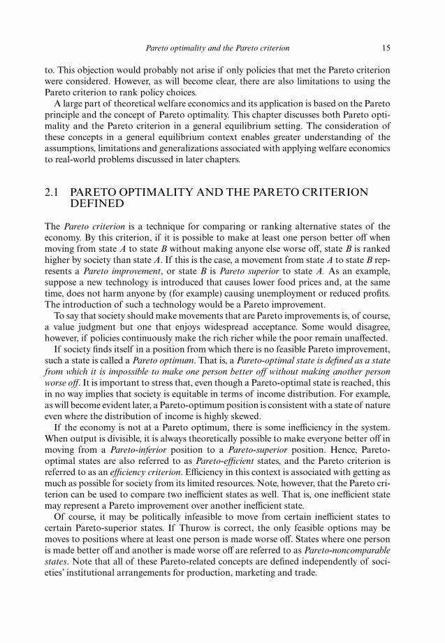
time, move OB, thus shifting B’s indifference map; but do this such that individual B’sindifference curve U1

B remains tangent to individual A’s indifference curve U1A with axes

for both goods parallel between individuals. Thus, C consists of the locus of all outputbundles to which every member of society is indifferent if the bundle is initially distrib-uted at point a.

Now consider comparing a particular distribution of one bundle of goods on the pro-duction possibility frontier with the distribution of another bundle also on the frontier.For example, in Figure 2.4 consider comparing the output bundle at OB, which is distrib-uted between individuals A and B at point a, with the output bundle at OB! distributed atpoint a!. The Scitovsky curves corresponding to the distribution at points a and a! are Cand C!, respectively. Note that C is not tangent to the production possibility curve at OBwhile C! is tangent at OB!. Both individuals can be made better off by choosing the bundleat OB! because C! lies above C and because only output at OB

* (instead of OB!) distributedat point a! is needed to yield the same level of total utility as at OB. The additional productq1

2 – q13 of q1 and q2

2 – q23 of q2 can be divided in any way desired to make both individu-

als better off in moving from OB* to OB!.

Even though C! lies entirely above C, however, both individuals need not be made actu-ally better off in moving from OB to OB! in Figure 2.4. That is, the bundle represented byOB! may be distributed at point b, where individual A is made better off and individual Bis worse off, relative to the bundle represented by OB, distributed at point a. The SICs canlie with one entirely above the other, and one individual may still be worse off at the higherSIC. However, it is possible to redistribute the output bundle at OB! to make everyonebetter off than at point a (the distribution of the initial bundle) by choosing a distributionof the product at OB! in the shaded region.

Now consider comparing output bundle OB! distributed at point a! (which generates theSIC denoted by C! tangent to PP!) with any other efficient output bundle with all pos-sible distributions. Because there are no feasible production points above C!, it is impos-sible to generate an SIC that lies above C!. That is, if one starts at OB! distributed at pointa!, one person cannot be made better off without making another person worse off. Inother words, OB! distributed at point a! is a Pareto-optimal point.

The requirement of tangency of the SIC to the production possibility curve thus estab-lishes a third set of marginal equivalences which must hold for Pareto optimality in theproduct-mix case. That is, the slope of the production frontier must be the same as theslope of the SIC at the optimum. But the negative of the slope of the production possibil-ity curve is the marginal rate of transformation of q1 for q2 (which measures the rate atwhich one output can be traded for another with given quantities of inputs), denoted byMRTq1q2, and the negative of the slope of the SIC is the marginal rate of substitution ofq1 for q2 for both individuals A and B. Thus, Pareto optimality in product mix implies thatthe marginal rate of transformation must be equal to the marginal rates of substitution forconsumers; that is,

MRTq1q2"MRSAq1q2"MRSB

q1q2. (2.3)

The intuition of this condition is clear because improvements for one individual are pos-sible without affecting any other individual if production possibilities are such that theincremental amount of one output that can be produced in place of one (marginal) unit


of another output is greater than the amount that some individual is willing to accept inplace of that one unit. Of course, this condition does not define a Pareto optimumuniquely. Any point on the production possibility frontier distributed such that the corre-sponding SIC is tangent to the production possibility curve satisfies the condition. And,as in the pure exchange case, the Pareto criterion does not provide a basis for choosingamong these points.

2.5 PARETO OPTIMALITY AND COMPETITIVEEQUILIBRIUM

Pareto optimality has thus far been examined independent of societies’ institutional arrange-ments for organizing economic activity. However, fundamental relationships exist betweenthe notion of Pareto optimality and the competitive market system as a mechanism for deter-mining production, consumption, and the distribution of commodities. In particular, whena competitive equilibrium exists, it will achieve Pareto optimality. Moreover, if producersand consumers behave competitively, any Pareto optimum can be achieved by choosing anappropriate initial income distribution and appropriate price vector.

Before these relationships can be demonstrated, the concept of competitive equilibriumfor a market system must be defined. Suppose that the economy consists of N tradedgoods, J utility-maximizing consumers and K profit-maximizing producers. Also, supposethat consumers and producers act competitively, taking prices as given. Let the demandsby consumer j follow by qj!qq j(p, m j)![q1

j(p, mj),...,qNj(p, mj)], which represents a vector

of quantities demanded of all goods by consumer j where p!(p1,...,pN) is a vector ofprices for all goods and mj is the income level of consumer j. In addition, let the suppliesof consumer goods by producer k be represented by qk!qqk(p, w) and let the demands forfactor inputs by producer k be represented by xk!xxk(p, w)![x1

k(p, w),...,xLk(p, w)] where

w!(w1,...,wL) is a vector of all input prices. Finally, suppose factor ownership is distrib-uted among consumers so that each consumer holds a vector of factor endowments xx j!(x1

j,...,xLj) and thus has income mj!"L

l!1 wl xlj. Then suppose there exist vectors of prices

p and w such that the sum of quantities demanded is equal to the sum of quantitiessupplied in all markets,

qq j(p,mj)! qqk(p,w),

xxk(p,w)! xx j.

The set of prices p and w then gives a competitive equilibrium.1 Thus, a competitive equi-librium is simply a set of prices such that all markets clear.

!J

j!1!

K

k!1

!K

k!1!

J

j!1


1. This definition of a competitive equilibrium assumes free entry so that profits of firms are driven to zero. Ifprofits are nonzero, then all profits must be distributed to consumers so that consumer j has income mj!"L

l!1 wlxlj#"K

k!1 sjk where sjk is the share of producer k profit received by consumer j such that "Jj!1 sjk!$k

where $k is the profit of firm k,

$k!"Nn!1pnqk

n%"Ll!1wlxk

l.

A competitive equilibrium can be shown to exist if (1) all consumers have preferencesthat can be represented by indifference curves that are convex to the origin, and (2) if noincreasing returns exist for any firm over a range of output that is large relative to themarket.2 Of course, many competitive equilibria may exist depending upon the distributionof factor ownership or consumer income.

The First Optimality Theorem

The first important relationship between competitive equilibrium and Pareto optimalityis that, when a competitive equilibrium exists, it attains Pareto optimality.3 This result, for-mally known as the first optimality theorem, is sometimes called the invisible handtheorem of Adam Smith (1937). In the Wealth of Nations, first published in 1776, Smithargued that consumers acting selfishly to maximize utility and producers concerned onlywith profits attain a best possible state of affairs for society, given its limited resources,without necessarily intending to do so. Although more than one best (Pareto-efficient)state of affairs generally exists, Smith was essentially correct.

To see this, first consider the case of consumer A displayed in Figure 2.5. To maximizeutility, given the budget constraint II! associated with income m, consumer A chooses theconsumption bundle (q1,q2) which allows him or her to reach the highest possibleindifference curve. Thus, the consumer chooses the point of tangency between II! and theindifference curve UA. At this tangency, MRSA

q1q2"p1/p2 because the former is the nega-tive of the slope of the indifference curve and the latter is the negative of the slope of thebudget constraint. But under perfectly competitive conditions, all consumers face thesame prices. Thus, MRSB

q1q2"p1/p2 for consumer B and, hence,

MRSAq1q2"MRSB

q1q2, (2.4)


2. The first condition is a standard assumption of economic theory and needs no further comment. Theproblem that arises with increasing returns is that the average cost curve for the firm is continuously decreas-ing and the marginal cost curve is always below the average cost curve. With falling average costs, if it paysthe firm to operate at all, then it pays the firm to expand its scale of operations indefinitely as long as outputprice is unaffected because the marginal revenue is greater than the marginal cost on each additional unitproduced. If increasing returns exist over a large range of output, the percentage of the industry output pro-duced by such a firm eventually reaches sufficient size to have an influence on price, and thus the firm willno longer be competitive. Hence, no profit-maximizing equilibrium exists for competitive firms in this case.As long as increasing returns are small, on the other hand, a competitive industry will consist of a greatnumber of firms with the usual U-shaped average cost curves, and all of these profit-maximizing firms willoperate at either the minimum or on the increasing portion of their average cost curve. For a rigorous devel-opment of the problem of existence and uniqueness of competitive equilibrium, see Quirk and Saposnik(1968) or Arrow and Hahn (1971).

3. Formally, this result requires that (1) firms are technologically independent and (2) consumers’ preferences areindependent. The first assumption implies that the output of each firm depends only on the input-use deci-sions it makes, and not on the production or input decisions of other firms other than quantities traded atcompetitive prices. The latter assumption implies that the utility function for each consumer contains as var-iables only items over which the consumer has a choice and not those quantities chosen by other consumersor producers other than quantities traded at competitive prices. Assumptions (1) and (2) jointly imply thatno externalities exist. For a rigorous proof of this result, see Quirk and Saposnik (1968) or Arrow and Hahn(1971). A detailed discussion is also given by Arrow (1970, pp. 59–73). It is possible for a competitive equi-librium to achieve Pareto optimality in the presence of externalities if efficient markets exist for all externaleffects. These possibilities are discussed in Chapter 13.

which is the Pareto-optimality exchange condition derived in equation (2.1). That is,because all consumers face the same relative prices of the two goods, their marginal eval-uations must be the same in equilibrium.4

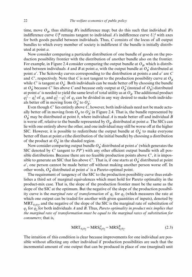
Now, recall that a firm cannot maximize profits for any level of output unless it is pro-ducing that output at a minimum cost. That is, profit maximization implies cost minimiza-tion. Assuming that q1 is the profit-maximizing level of output for the firm producing q1in Figure 2.6, the minimum cost of producing this output given input prices w1 and w2 isobtained by using x1 of x1 and x2 of x2. That is, the cost-minimizing input bundle isselected by finding the point of tangency of the isocost curve CC! (associated with costlevel c) with the isoquant associated with output q1"q1. Finding this point of tangencyinvolves equating the slope of the isoquant, which is equal to the negative of the rate oftechnical substitution of x1 for x2, with the slope of the isocost curve, which is equal to


4. To develop this result more generally mathematically, let consumer j have utility function Uj(qj) assumedto satisfy usual monotonicity, quasiconcavity, and differentiability properties. The consumer’s budgetconstraint is then mj"pqj"#N

n"1pnqnj, the Lagrangian of the utility maximization problem is Uj(qj)

$ %(mj $ pqj), and the first-order conditions are &Uj/&qnj $%pn"0, n"1, ..., N. Note that the demand func-

tions qj"qq j(p, mj) must satisfy these first-order conditions. Taking ratios of pairs of first-order conditionsimplies that consumer behavior satisfies

MRS jqnqn!

! " .pn

pn!

&Uj/&qjn

&Uj/&qjn!

Figure 2.5

q1 m/p1 q1

q2

m/p2

q2

Slope = –MRSAq1q2

I ' U A

p1Slope = – — p2

I

the negative of the ratio of input prices. But all producing firms that use x1 and x2 facethe same input prices. Hence,

RTSq2x1x2!RTSq1x1x2

, (2.5)

which yields the production efficiency condition of equation (2.2).5To establish that the product-mix condition of equation (2.3) is satisfied, first consider

increasing the output of q1 by "q1 and decreasing the output of q2 by "q2 along the pro-duction possibility curve. Suppose this change is accomplished by transferring at themargin either one unit of x1 or one unit of x2 from production of q2 to production of q1.Then, the increase in output of q1 is equal to the marginal physical product of input xk inproduction of q1. That is, "q1!MPPq1xk

. Similarly, the decrease in output of q2 is "q2!MPPq2xk

. But the amount of q2 that must be given up to obtain an increment of q1 is givenby the marginal rate of transformation between q1 and q2. Thus,6


5. To develop this result more generally mathematically, let producer k have short-run profit represented by #k

!pqk$wxk!%Nn!1 pnqn

k$%Ll!1 wlxl

k, and implicit production function f k(qk,xk)!0 where f k is assumed tosatisfy usual monotonicity, concavity and differentiability properties. Then the Lagrangian of the profitmaximization problem is pqk – wxk&'[f k(qk, xk)] and the first-order conditions are '((f k/(qn

k)&pn!0, n!1, ... , N, and '((f k/(xl

k) – wl!0, l!1, ... , L. Because all producer supplies and demands must satisfy thesefirst-order conditions, taking appropriate ratios of pairs of first-order conditions implies

RTSkxlxl)

! ! .

6. The first-order conditions of footnote 5 also imply

MRTkqnqn)

! ! ,

which generalizes the result in equation (2.6).

pn)

pn

(f k/(qkn)

(f k/(qkn

wl

wl)

(f k/(xkl

(f k/(xkl)

Figure 2.6

x1 c / w1 x1

x2

q1 = q1

x2

Slope = –RTSq1x1x2

w1Slope = – — w2

Cc/w2

C'Oq1

MRTq1q2! ! . (2.6)

Now recall that cost minimization by a producer requires that producers equalize themarginal physical product per dollar spent on each input. That is, the least-cost combina-tion x1, x2 in Figure 2.6 is characterized by the conditions

! , j!1, 2. (2.7)

But the marginal physical product of an input is equal to the increase in output "qjdivided by the increase in input "xk required to obtain the increase in output. Thus, MPPqj

xk!"qj/"xk. Using this result in equation (2.7) and inverting yields

w1 !w2 , j!1, 2, (2.8)

where wk "xk/"qj is simply the marginal cost, MCqj, of obtaining an additional unit of qj.

Combining (2.7) and (2.8) thus yields

MCqj! j!1, 2. (2.9)

Finally, recall that all profit-maximizing producers equate marginal revenue, which issimply the competitive producer’s output price, with marginal cost. Thus, substituting pjfor MCqj

in equation (2.9) and dividing the equation with j!1 by the one with j!2 yields7

! . (2.10)

But from equation (2.6), the right-hand side of equation (2.10) is simply MRTq1q2. Because

consumers face these same commodity prices, the product-mix condition in equation(2.3),

MRTq1q2!MRSA

q1q2!MRSB

q1q2, (2.11)

must hold with competitive market equilibrium.Thus, under the assumptions of this chapter, competition leads to conditions (2.4),

(2.5), and (2.11), which are identical to conditions (2.1)–(2.3) that define a Paretooptimum. In other words, competitive markets are Pareto efficient, meaning that competi-tive markets result in an equilibrium position from which it is impossible to make a changewithout making someone worse off. This conclusion is probably the single most powerful

MPPq2xk

MPPq1xk

p1

p2

wk

MPPqjxk

"x2

"qj

"x1

"qj

MPPqjx2

w2

MPPqjx1

w1

MPPq2xk

MPPq1xk

"q2

"q1


7. To obtain equation (2.10) from equation (2.6) generally, note that comparative static analysis of the produc-tion function constraint in footnote 5 holding all but one input and all but one output constant yields

!# .

Using this and a similar relationship for dqn$k/dxk

i in the equation of footnote 6 reveals that

MRTkqnqn$

! ! ! .

The result in equation (2.11) follows because each term is equal to the same price ratio.

pn$

pn

%f k/%qkn$

%f k/%qkn

dqkn/dxk

l

dqkn$/dxk

l

%f k/%xkl

%f k/%qkn

dqkn

dxkl

result in the theory of market economies and is widely used by those economists whobelieve that markets are competitive and, hence, that government should not intervene ineconomic activity. Milton Friedman and the ‘Chicago School’ are the best known defend-ers of this position (see Friedman and Friedman 1980). In addition, because of itsefficiency properties, competitive equilibrium offers a useful standard for policy analysis.For this purpose, states of competitive equilibrium or Pareto optimality are called first-best states and the associated allocations are called first-best bundles. All other states orbundles are called second-best. Departures from competitive equilibria are called marketfailures. Examples of market failures include monopolistic behavior, taxes, and external-ities. Policies that correct market failures are thus viewed as achieving competitive equi-librium and therefore attain economic efficiency.

The Second Optimality Theorem

The second optimality theorem states that any particular Pareto optimum can be achievedthrough competitive markets by simply prescribing an appropriate initial distribution offactor ownership and a price vector.8 That is, a central planner can achieve any efficient pro-duction bundle and any distribution of consumer well-being by redistributing factor own-ership and prescribing appropriate prices where consumers maximize utility subject tobudget constraints and producers maximize profits. The use of the competitive mecha-nism in this manner is sometimes called Lange–Lerner socialism after the two economistswho first recognized this possibility (see Lange 1938; Lerner 1944). This result implies thatmany Pareto optima exist which are competitive equilibria, each associated with differentfactor endowments. The potential for widely differing marginal valuations under alterna-tive competitive equilibria illustrates the connection between efficiency and income distri-bution.

Many economists object to addressing efficiency and distribution in two stages wherethe first stage involves maximizing economic efficiency and the second stage involves dis-tributing the product equitably. The relative value of products depends on income distri-bution, which depends, in turn, on the factor ownership distribution. Actually, theLange–Lerner result suggests the opposite approach whereby distributional objectivescan be achieved by first redistributing factor ownership. Then policies need to be adoptedonly to correct market failures in order to achieve a Pareto optimum consistent with thedesired income distribution.

Figure 2.7 demonstrates this point by considering only two possible states. The twogoods produced are q1 and q2, and PP! is the production possibility frontier. TheScitovsky indifference curve C pertains to the output bundle OB distributed among theindividuals at point a. Alternatively, the output bundle OB! distributed at point b yields theScitovsky indifference curve C!. As points OB and OB! show, both bundles and their dis-tributions lead to Pareto-optimal states. Thus, points OB and OB!, with corresponding dis-tributions at points a and b, respectively, are called first-best states, but neither is a uniqueoptimum because the other is also an optimum in the same sense. For example, a factorownership distribution that produces competitive equilibrium at point a may leave theeconomy poorly suited to achieve a distributional objective consistent with point b. On


8. For a rigorous proof of this result, see Quirk and Saposnik (1968) or Arrow and Hahn (1971).

the other hand, starting from a factor ownership distribution that generates consumerincomes consistent with point b, the Lange–Lerner result implies that a Pareto efficientorganization will be achieved automatically by the Adam Smith invisible hand in absenceof market failures.

2.6 LIMITATIONS OF PARETO OPTIMALITY AND THEPARETO PRINCIPLE

Although the Pareto principle gives a plausible criterion for comparing different states ofthe world, its limitations are numerous. The greatest shortcoming of the Pareto principleis that many alternatives are simply not comparable. For example, in Figure 2.8, if pro-duction possibilities are represented by PP and production is initially OB with distribu-tion at point b corresponding to Scitovsky indifference curve C, then the onlyPareto-preferred alternatives are in the shaded, lens-shaped area. All other productionpoints are either infeasible, non-Pareto comparable or Pareto inferior. If production is ini-tially at OB with distribution at point a corresponding to Scitovsky indifference curve C!,then no other feasible alternatives are Pareto superior. In fact, once any competitive equi-librium is reached in the framework of this chapter, no other feasible alternatives arePareto superior. For example, production at OB with distribution corresponding to theScitovsky indifference curve C! is not Pareto comparable to production at OB! with distri-bution corresponding to social indifference curve C*. Thus, alternative Pareto optima are


Figure 2.7

q11 q1

2 q1

q2

P

OB'

OA

P'C'

b

a

OB

C

q21

q22

not Pareto comparable. Hence, the Pareto criterion prevents consideration of income-distributional considerations once a competitive equilibrium is attained.

Another serious problem with the Pareto principle is that no unique choice of distribu-tion is apparent when improvements are possible. For example, suppose that a technolog-ical change takes place in Figure 2.8, shifting the production possibility frontier out toP!P!. If production was initially at OB with distribution at point a corresponding toScitovsky indifference curve C!, the only points that are Pareto superior are those aboveC! and below or on P!P!. The only points that are Pareto superior and also possibly cor-respond to Pareto optimality with the new technology are those on the P!P! frontierbetween OB

* and OB**. But the points along this interval may be associated with a wide

variation in income distribution (assuming, for example, that only one distribution existsat each production point with tangency between the Scitovsky indifference curve and thenew production possibility frontier). The Pareto criterion gives no basis for choosingamong these alternatives. However, this problem may be viewed as an advantage becausepossibilities can exist for altering income distribution while fulfilling the simply appealingnature of the Pareto criterion. For example, in a rapidly growing economy (one withrapidly expanding production possibilities), the possibilities for altering income distribu-tion while still fulfilling the Pareto criterion are many even though the Pareto criteriongives no guidance on which income distribution should be chosen.

Even with expanding production possibilities, however, the Pareto principle stronglyfavors the status quo. For example, if production is originally at OB with distribution asso-ciated with Scitovsky indifference curve C!, a new point of Pareto optimality is possible


Figure 2.8

q1

q2P'

OB'

OA

P'

C'

b

a

OB

C

OB**

OB+

OB++

C*P

OB*

P

only at points between OB* and OB

** on the new frontier P!P! in Figure 2.8, assuming thatthe Pareto principle is satisfied in such a change. But if the initial production point is atOB! with distribution associated with Scitovsky indifference curve C*, a new Paretooptimum is possible only at points between OB

" and OB"" on the frontier P!P!, again

assuming the Pareto principle is satisfied in the change. In each case the set of feasiblePareto improvements does not represent a substantial departure from the initial pointunless technological improvements are large. Again, alternatives with widely varyingincome distributions may be neither comparable nor attainable from a given initial stateby strict adherence to the Pareto criterion.

In a policy context, decisions often must be made where someone is made worse offwhile someone else is made better off. Furthermore, some policies are directly intended tochange the distribution of income (that is, narrow the gap between high- and low-incomepeople). Hence, to evaluate such changes, a device other than the Pareto principle isneeded.

2.7 CONCLUSIONS

This chapter has focused on the concept of Pareto optimality and the Pareto criterion. APareto improvement is a situation where a move results in at least one person becomingbetter off without anyone becoming worse off. Pareto optimality is achieved when it is nolonger possible for a policy change to make someone better off without making someoneelse worse off.

From a policy point of view, the Pareto criterion favors the status quo because the rangeof choices that represent Pareto improvements depends critically on the initial distribu-tion of income. The Pareto criterion cannot be used to choose among widely differentincome distributions. Furthermore, many Pareto-optimal policy choices may exist thatcorrespond simply to different income distributions. Perhaps not all first-best, Pareto-optimal choices are superior to some particular second-best choice. Although it is pos-sible to make a Pareto improvement from a second-best state, it does not follow that anyPareto-optimal state is preferred to any second-best state. For example, if a second-bestand a first-best state have markedly different income distributions, the situation that issecond best may not be inferior to the first-best situation. Thus, the Pareto criterion aloneappears to constitute an insufficient basis for applied economic welfare analysis of publicpolicy alternatives.


3. The compensation principle and the welfarefunction

In Chapter 2, emphasis was given to the Pareto criterion as a means for selecting amongalternative policies. Results show that many ‘first-best’ bundles or many Pareto-optimalpoints usually exist for an economy but, unfortunately, the Pareto principle does not givea basis for selecting among them. Narrowing the range of possibilities to a single first-bestbundle (which essentially requires determining the ideal income distribution) requires amore complete criterion. One such criterion, which was introduced much later than thePareto principle in the hope that it would be a more powerful device for choosing amongpolicies, is the compensation principle, sometimes called the Kaldor–Hicks compensationtest after the two economists to which it is attributed (Kaldor 1939; Hicks 1939). Thedevelopment of the compensation principle was thus an attempt to broaden the states ofthe world that could be compared using an accepted welfare criterion. Simply stated, stateB is preferred to state A if at least one individual could be made better off without makinganyone worse off at state B – not that all individuals are actually no worse off – by somefeasible redistribution following the change. Unlike the Pareto principle, the compensa-tion criterion does not require the actual payment of compensation.

The issue of compensation payments is at the heart of many policy discussions. Someargue that compensation should be paid in certain cases. According to Lester Thurow(1980, p. 208), ‘If we want a world with more rapid economic change, a good system oftransitional aid to individuals that does not lock us into current actions or current insti-tutions would be desirable.’ However, most policies that have been introduced have notentailed compensation. For example, bans on DDT and other pesticides have in manycases resulted in producer losses, but producers have not been compensated for their lossesin revenue.

Although the compensation principle does, in fact, expand the set of comparable alter-natives (at the expense of additional controversy), some states remain noncomparable.The latter part of this chapter considers the necessary features of a criterion that ranksall possible states of an economy. However, empirical possibilities for the resulting moregeneral theoretical constructs appear bleak.

3.1 THE COMPENSATION PRINCIPLE

According to the compensation principle, state B is preferred to state A if, in making the movefrom state A to state B, the gainers can compensate the losers such that at least one person isbetter off and no one is worse off. Such states are sometimes called potentially Pareto pre-ferred states. The principle is stated in terms of potential compensation rather than actualcompensation because, according to those who developed the principle, the payment of

32

compensation involves a value judgment. That is, to say that society should move to stateB and compensate losers is a clearly subjective matter, just as recommendation for changeon the basis of the Pareto criterion is a subjective matter. For example, if a Pareto improve-ment is undertaken, then, as demonstrated in Section 2.6, the possibilities that representfurther Pareto improvements may be more restricted. Conceivably, the true optimum stateof society may not be reachable by further applications of the criterion if the wrong initialPareto improvement is undertaken. Similarly, to say that society should move to state Bwithout compensating losers is also a subjective matter of perhaps a more serious nature.Thus, nonpayment of compensation also involves a value judgment. In terms of objectivepractice, one can only point out the potential superiority of some state B without actuallymaking a recommendation that the move be made.

The Pure Consumption Case1

Consider the application of the compensation principle to comparing different distribu-tions of a given bundle of goods, again using the basic model of two goods and two indi-viduals developed in Chapter 2. In Figure 3.1, point a is preferred to point b on the basisof the Pareto principle. But how does one compare point b with a point such as c, wherec is not inside the lens-shaped area? The compensation principle offers one possibility.For example, suppose that one redistributes the bundle such that, instead of being atpoint b, individual A is at point d and individual B is at point e. Note that the welfare ofeach is unchanged. However, at these points there is an excess of q2 equal to q2

3!q22

and an excess of q1 equal to q13!q1

2. Now, if the move actually takes place to point c,

The compensation principle and the welfare function 33

1. This section is largely based on Bailey (1954).

Figure 3.1

q11 q1

2OA

b

c

q22

q13

Good q1

Goo

d q 2

q23

q21

OB

da

e

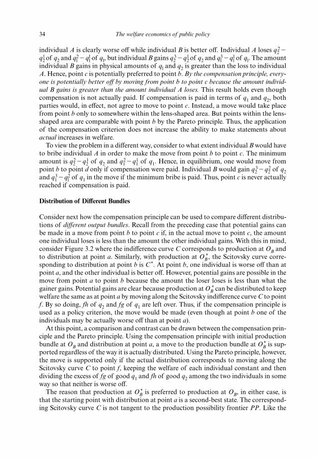
individual A is clearly worse off while individual B is better off. Individual A loses q22!

q2l of q2 and ql

2!qll of ql, but individual B gains q2

3!q2l of q2 and ql

3!qll of ql. The amount

individual B gains in physical amounts of ql and q2 is greater than the loss to individualA. Hence, point c is potentially preferred to point b. By the compensation principle, every-one is potentially better off by moving from point b to point c because the amount individ-ual B gains is greater than the amount individual A loses. This result holds even thoughcompensation is not actually paid. If compensation is paid in terms of q1 and q2, bothparties would, in effect, not agree to move to point c. Instead, a move would take placefrom point b only to somewhere within the lens-shaped area. But points within the lens-shaped area are comparable with point b by the Pareto principle. Thus, the applicationof the compensation criterion does not increase the ability to make statements aboutactual increases in welfare.

To view the problem in a different way, consider to what extent individual B would haveto bribe individual A in order to make the move from point b to point c. The minimumamount is q2

2!q21 of q2 and q1

2!q11 of q1. Hence, in equilibrium, one would move from

point b to point d only if compensation were paid. Individual B would gain q23!q2

2 of q2and q1

3!ql2 of q1 in the move if the minimum bribe is paid. Thus, point c is never actually

reached if compensation is paid.

Distribution of Different Bundles

Consider next how the compensation principle can be used to compare different distribu-tions of different output bundles. Recall from the preceding case that potential gains canbe made in a move from point b to point c if, in the actual move to point c, the amountone individual loses is less than the amount the other individual gains. With this in mind,consider Figure 3.2 where the indifference curve C corresponds to production at OB andto distribution at point a. Similarly, with production at OB

*, the Scitovsky curve corre-sponding to distribution at point b is C*. At point b, one individual is worse off than atpoint a, and the other individual is better off. However, potential gains are possible in themove from point a to point b because the amount the loser loses is less than what thegainer gains. Potential gains are clear because production at OB

* can be distributed to keepwelfare the same as at point a by moving along the Scitovsky indifference curve C to pointf. By so doing, fh of q2 and fg of q1 are left over. Thus, if the compensation principle isused as a policy criterion, the move would be made (even though at point b one of theindividuals may be actually worse off than at point a).

At this point, a comparison and contrast can be drawn between the compensation prin-ciple and the Pareto principle. Using the compensation principle with initial productionbundle at OB and distribution at point a, a move to the production bundle at OB

* is sup-ported regardless of the way it is actually distributed. Using the Pareto principle, however,the move is supported only if the actual distribution corresponds to moving along theScitovsky curve C to point f, keeping the welfare of each individual constant and thendividing the excess of fg of good q1 and fh of good q2 among the two individuals in someway so that neither is worse off.

The reason that production at OB* is preferred to production at OB, in either case, is

that the starting point with distribution at point a is a second-best state. The correspond-ing Scitovsky curve C is not tangent to the production possibility frontier PP. Like the


Pareto criterion, the compensation principle does not support a move away from a first-best state such as production at OB

* with distribution point c corresponding to Scitovskyindifference curve C!. Thus, the compensation criterion, like the Pareto criterion, cannotbe used to rank two first-best states. A movement from one to the other would not be sup-ported regardless of which is used as a starting point. The compensation criterion, on theother hand, gives a means of comparing all pairs of second-best states and for compar-ing all second-best states with all first-best states.

The Reversal Paradox

An important class of problems in applying the compensation principle falls under thegeneral heading of the reversal paradox pointed out by Scitovsky (1941). For the casewhere gainers can potentially compensate losers, a conclusion that one position is betterthan another is not always warranted. One must ask, also, whether the losers can bribe thegainers not to make the move. The crux of the argument is presented in Figure 3.3. Theproduction possibility curve is PP, and the two bundles to be compared are OB and OB

*.Each of the bundles is distributed such that the corresponding Scitovsky indifferencecurves cross. In other words, both are second-best states because neither indifference curveis tangent to the production possibility curve. The curves C1 and C2 correspond to pointsa and c on the contract curves, respectively. Now, by the compensation principle, produc-tion at OB

* with distribution at point c is better than production at OB with distribution atpoint a because production at OB

* can generally be redistributed such that all are actually


Figure 3.2

q11 q1

2 q1

q2

P

OA

P

C'

a

OB

C

q21

q22

c

b

f g

h

C*

OB*

better off at point d (where distribution at point d corresponds to Scitovsky curve C2!,which lies above curve C1 and is associated with improved welfare for both individuals).However, by this criterion, OB

* is only potentially better off. Compensation is not actuallypaid. Because compensation is not actually paid, a reversal problem arises. That is, thenew state with production at OB

* and distribution at point c is a second-best state withScitovsky curve C2. Thus, according to Figure 3.3, there must be some distribution – say,at point b – such that production at OB is preferred to production at OB

* by the Scitovskycriterion (where distribution at point b corresponds to the Scitovsky curve C1!, which isassociated with improved welfare for both individuals as compared with C2). Thus, eachis preferred to the other.

This reversal occurs because in each case a given distribution of the first bundle is com-pared with all possible distributions of the alternative bundle. The reversal paradox sug-gests that all distributions of the initial bundle should also be considered. In other words,a reversal test (sometimes called the Scitovsky reversal test) is passed if one determines,first, that gainers can bribe losers to make a change and, second, that losers cannot bribegainers not to make the change. Unless the reversal test is passed in addition to theKaldor–Hicks compensation test, one cannot really say that one state is even potentiallypreferred to another.

Some additional points that must be borne in mind with respect to the Scitovsky rever-sal paradox are as follows:


Figure 3.3

q11 q1

2 q1

q2

P

OA

P

C2'

a

OB

C2

q21

q22

c

b

d

OB*

C4

C1'

OB'

C3

C1

1. The reversal paradox occurs only in comparing two second-best bundles. It does notarise if one of the bundles is a first-best or Pareto-efficient bundle. For example, inFigure 3.3, if production at OB

* with distribution corresponding to indifference curveC2 is compared to production at OB! with distribution corresponding to indifferencecurve C3, a reversal problem does not occur.

2. The reversal paradox does not always occur in comparing two second-best bundles eventhough compensation is not actually paid. For example, in Figure 3.3, production atOB

* with distribution corresponding to Scitovsky indifference curve C4 does not leadto a paradox when compared to production at OB and distribution corresponding toScitovsky curve C1. The paradox occurs only when the relevant Scitovsky curves crossin the interior of the feasible production region. This problem may not occur whenincome distributions do not change substantially.

Intransitive Rankings

If the compensation criteria (both the direct Kaldor–Hicks and Scitovsky reversal tests)are employed to rank all possible states, a further problem can arise even if the reversalproblem is not encountered. That is, compensation tests can lead to intransitive welfarerankings when more than two states are compared.2 This problem arises when, forexample, one must choose among, say, states where all the alternative policies are of asecond-best nature (that is, there is no single policy in the policy set that leads to a bundleof goods distributed with the Scitovsky community indifference curve tangent to the pro-duction possibility curve). In Figure 3.4, given the production possibility curve PP,bundle OB

2 is preferred to OB1, OB

3 is preferred to OB2 and bundle OB

4 is preferred to OB3,

using the compensation test. However, OB1 is also preferred to OB

4. Hence, the Kaldor–Hicks compensation test leads to welfare rankings that are intransitive. But note thatsome form of distortion exists for each bundle because the Scitovsky indifference curvesare not tangent to the production possibility curve in any of the four cases. All the bundlesare of a second-best nature.

Suppose, on the other hand, that one policy results in a bundle of goods that is eco-nomically efficient (with the Scitovsky indifference curve tangent to the production pos-sibility curve). For example, consider bundles OB

1, OB2, OB

3 and OB5. Here, OB

5 is clearly theoptimum choice. There is no desire, once at OB

5, to return to bundles OB1, OB

2 or OB3. As a

second example, suppose that the bundles to be compared are OB1, OB

2, OB3 and OB

6. Again,once at OB

6, no potential gain is generated in returning to OB1, OB

2 or OB3. Hence, no ambi-

guity is encountered in choosing a top-ranked policy if the policy set contains exactly onefirst-best state. Thus, as with the reversal problem discussed earlier, intransitivity occursonly when all the bundles being compared are generated from second-best policies.3

Consider, on the other hand, one further case where the possibilities consist of OB1, OB

5

and OB6. In this case, the Kaldor–Hicks compensation test shows that OB

5 is preferred to


2. The results in this section are due to Gorman (1955).3. Partly in response to the problems associated with using the compensation principle as a basis for welfare

comparison, Arrow (1951) developed the impossibility theorem, which proves that no reasonable ruleexists for combining rankings of various states of society by individuals into a societal ranking. See thefurther discussion in Section 3.4.

OB1. The possibility associated with OB

6 is not preferred to OB1 even though OB

6 is a first-best bundle. Among these three states, however, the rankings are not complete because,once at either OB

5 or OB6, the compensation test does not suggest a move to either of the

other states. In other words, the compensation test does not lead to a ranking of policysets containing more than one first-best state.

3.2 UTILITY POSSIBILITY CURVES AND THE POTENTIALWELFARE CRITERION

Another approach related to the choice of alternative income distributions and the rever-sal problem is based on the concept of utility possibility curves introduced by Samuelson(1947, 1956). To develop this approach, consider Figure 3.5 where the utilities of two indi-viduals, A and B, are represented. The utility of individual B is measured on the verticalaxis, while that for individual A is measured along the horizontal axis. Three utility pos-sibility curves are represented, each of which is derived by changing the distribution of agiven bundle of goods along a contract curve. For example, Q2Q2 shows the maximumutility both individuals can receive from a fixed production at OB in Figure 3.3, Q1Q1 cor-responds to a different bundle of goods, and so on.

To demonstrate the reversal paradox, consider Q2Q2 and Q1Q1. Points a and b repre-sent particular distributions of the bundle from which Q2Q2 is derived. Similarly, pointsc and d represent particular distributions of the bundle from which Q1Q1 is derived.


Figure 3.4

q1

q2

OA

P

C2

C6

OB4

C3C1

OB3

OB6

OB5

C5

OB2OB

1

C4P

Suppose that the initial distribution is at point c. Then one can redistribute productionwhen moving from Q1Q1 to Q2Q2 such that both individuals A and B would be better offat point b than at point c. Similarly, one could redistribute the other bundle so that bothare better off at point d than at point a. The paradox arises because point d lies to thenortheast of point a, while point b lies to the northeast of point c. Thus, one comparisonimplies a preference for the production bundle associated with Q1Q1, whereas the othercomparison favors the production bundle associated with Q2Q2. This paradoxical situa-tion would not arise if compensation were actually paid.

These results correspond directly with the analysis in commodity space in Figure 3.3.Points a and c in Figure 3.5 correspond to distributions that are second-best states. Inother words, these points correspond to points a and c in Figure 3.3, which are also dis-tributions giving rise to second-best states. Note that points b and d in Figure 3.5 andpoints b and d in Figure 3.3 correspond to first-best states.

If one considers all possible production bundles that can be obtained from a givenproduction possibility frontier and all possible distributions of these bundles (which, inutility space, corresponds to considering utility possibility frontiers, such as Q3Q3, asso-ciated with all other possible production bundles), then the grand utility possibility fron-tier UU can be constructed as an envelope of the utility possibility frontiers. All points onthis envelope curve correspond to first-best optima, that is, bundles distributed such thatthe Scitovsky curves are tangent to the production possibility curve.


Figure 3.5

UB

OA

U

eQ1

b

c

da

U

Q4

Q2

Q3

Q2 Q1 Q3 Q4 UA

W0

Samuelson (1950) has argued that even if gainers can profitably bribe losers into accept-ing a movement and the losers cannot profitably bribe the gainers into rejecting it (that is,both the Kaldor–Hicks and Scitovsky criteria are satisfied), a potential gain in welfare isnot necessarily attained. He argues that one has to consider all possible bundles and allpossible distributions of these bundles before statements can be made about potentialgains. The problem then amounts to selecting one among many first-best states for whichthere is no solution unless a social ranking of first-best utility possibilities can be deter-mined. He proposes an alternative potential welfare criterion, which is demonstrated inFigure 3.5. Simply stated, if there is some utility frontier such as Q4Q4 that lies entirely onor outside another utility frontier – Q2Q2, for example – owing perhaps to technologicalchange, then any position on this new frontier is clearly at least potentially superior to anyposition on the old one. Only if the new frontier lies entirely outside the other, however, arepotential increases in real income necessarily obtained. Of course, this criterion can beused to compare either grand utility possibility frontiers before and after, say, a techno-logical change or utility possibilities associated with given alternative production bundles.

In the absence of a rule for ranking alternative first-best utility possibilities, Samuelson(1950) argues that this is the only appropriate criterion to apply. In a strict sense, this argu-ment is correct. But in a practical sense, this approach leads to few cases in whichbeneficial empirical evidence can be developed for policy-makers (see Section 8.3 for a dis-cussion of the related empirical approach). On the other hand, the arguments in favor ofthis approach are based on an attempt to determine optimal policy without relying onpolicy-maker preferences or judgment. Such information is not necessary in a practicalpolicy-making setting where political institutions exist for the express purpose of provid-ing policy-makers to make such choices.

3.3 THE SOCIAL WELFARE FUNCTION

Because the potential welfare criterion often may not be satisfied even if utility possibil-ity curves can be identified, economic inquiry has continued to search for a rule that canrank all states of society and thus determine which first-best state on the grand utility pos-sibility frontier represents the social optimum. In theory, the social welfare function issuch a concept. The social welfare function is simply a function – say, W(UA,UB) – of theutility levels of all individuals such that a higher value of the function is preferred to alower one. The assumption that the social welfare function is determined by the utilitiesof all individuals has been called the fundamental ethical postulate by Samuelson (1947)and is a cornerstone of democratic societies. Such a welfare function is called a Bergsonianwelfare function after Abram Bergson (1938), who first used it.

The properties one would expect in such a social welfare function with respect to theutilities of individuals are much like those one would expect in an individual’s utility func-tion with respect to the quantities of commodities consumed. That is, one would expectthat (1) an increase in the utility of any individual holding others constant increases socialwelfare (the Pareto principle); (2) if one individual is made worse off, then another indi-vidual must be made better off to retain the same level of social welfare; and (3) if someindividual has a very high level of utility and another individual has a very low level ofutility, then society is willing to give up some of the former individual’s utility to obtain


even a somewhat smaller increase in the latter individual’s utility, with the intensity of thistrade-off depending upon the degree of inequality.

The properties described above suggest the existence of welfare contours such as W0 inFigure 3.5, which correspond conceptually to indifference curves for individual utilityfunctions. By property (1), social welfare increases by moving to higher social welfare con-tours, either upward or to the right. By property (2), the social welfare contours have neg-ative slope. By property (3), the welfare contours are convex to the origin.

Social welfare is maximized by moving to the highest attainable social welfare contour,which thus leads to tangency of the grand utility possibility frontier with the resultingsocial welfare contour such as at point e in Figure 3.5.4 This tangency condition is some-times called the fourth optimality condition. This condition, together with conditions inequations (2.1), (2.2) and (2.3), completely characterizes the social optimum.

3.4 LIMITATIONS OF THE SOCIAL WELFARE FUNCTIONAPPROACH

Although a social welfare function is a convenient and powerful concept in theory, itspractical usefulness has been illusory. Many attempts have been made to specify a socialwelfare function sufficiently to facilitate empirical usefulness but none have been widelyaccepted. Apparently, little hope exists for determining a social welfare function on whichgeneral agreement can be reached. The major approaches that have been attemptedinclude (1) the subjective approach, (2) the basic axiomatic approach and (3) the moraljustice approach.

The subjective approach is represented by those who postulate a complete functionalform for the social welfare function on subjective ethical grounds. Early students of theutilitarian school (for example, Bentham 1961, first published 1823) believed that changesin happiness should simply be added over individuals,

W!U1"U2"U3"… (3.1)


4. Note that the slope of the welfare contour can be represented by

# !#

if W(UA, UB) is continuous and first derivatives exist. The slope of the utility possibility frontier is

# !# .

Thus, the tangency condition can be represented mathematically by

! , i!1, 2.

Cross-multiplying yields

! , i!1, 2,

which, simply stated, implies that the marginal social significance of consumption must be equated acrossindividuals for each commodity.

"$UA

$qi#$W

$UA"$UB

$qi#$W

$UB

$UB /$qi

$UA /$qi

WUA

WUB

$UB/$q2

$UA/$q2

$UB/$q1

$UA/$q1

WUA

WUB

$W/$UA

$W/$UB

where Ui represents the utility of individual i. A positive net gain is then viewed as groundsfor policy implementation. This implies that the welfare contours such as W0 in Figure3.5 should be straight lines with slope !1. Others argue that a functional form should beused that reflects positive benefits from increases in equality consistent with ‘normal’ dis-tributional judgments (see, for example, Blackorby and Donaldson 1990). One socialwelfare function that reflects inequality aversion is the form,

W" [(U1)1!#$(U2)1!#$(U3)1!#$…]. (3.2)

The problem here is that the term ‘normal’ is ambiguous. For example, agreement cannotbe reached on the appropriate level of inequality aversion, for example, the appropriatevalue of # in equation (3.2).5

The axiomatic approach, on the other hand, attempts to investigate the existence andform of the social welfare function mathematically based on a set of plausible underlyingaxioms about individual preferences and how they count to society. The most celebratedof these efforts is Arrow’s (1951) impossibility theorem. This theorem addresses the ques-tion of whether a general rule exists that can rank social states based only on the way thesestates are ranked by individual members of society. Arrow showed that no such rule existsunder the following plausible requirements:

1. The domain of decisions is unrestricted.2. The Pareto principle applies.3. Dictatorship is ruled out.4. Rankings are independent of irrelevant alternatives.

An example of a rule that does not work is majority voting. Arrow’s (1951) results suggestthat social preferences are determined by a dictator (or a group that acts as a dictator),that the intensity of preferences of individuals rather than simple rankings matters (seeKemp and Ng 1977), or that one of the other axioms such as independence of irrelevantalternatives does not apply (see Sen 1970). Accordingly, Arrow’s work has spawned a volu-minous literature on possibility theorems by relaxing his axioms in various ways (see Sen1982 or Fishburn 1973 for surveys). A major practical problem with this approach is thateven under weaker axioms where voting works, the transactions costs of compiling votesor rankings of all individuals on each policy issue are prohibitive.

The moral justice approach argues that basic axiomatic examinations following Arrowfail because majority groups acting selfishly will prefer to eliminate consideration ofminority interests. This failure can be addressed by admitting moral considerations suchas impartiality and economic justice. Suppose that society consists of three individuals anda change is considered that takes $1000 from one individual to give $300 to each of theother two. If the three individuals were to vote selfishly knowing who the benefactors are,the majority would favor the change. On the other hand, if the voting were done notknowing who would pay and who would receive (a veil of ignorance), then the change

11 ! #


5. To demonstrate the different inequality aversions possible with the function in equation (3.2), note that itreduces to (3.1) when #"0, it approaches (3.4) below when # approaches infinity, and it approaches themultiplicative form, W"U1U2U3… when # approaches 1. See Boadway and Bruce (1984, ch. 5).

would be unanimously rejected. Alternatively, moral concerns for equal treatment of indi-viduals (impartiality) have led some to support value judgments whereby the socialwelfare function treats individuals symmetrically, for example, W(UA,UB)!W(UB,UA).The contours of the social welfare function in Figure 3.5 are then symmetric about a 45°line from the origin. If all individuals have identical utility functions then the utility pos-sibility frontier is also symmetric about the 45° line and optimality is achieved by perfectequality. On the other hand, if one individual receives proportionally more utility fromconsuming the same bundles of goods as another, then such a welfare function would, ineffect, assign different weights to the consumption of the individuals.

Harsanyi (1953, 1955) gave the first formal treatment of moral considerations by dis-tinguishing between an individual’s personal preferences and moral preferences. In hiswork, moral preferences are the rankings of a rational individual given that the individ-ual does not know which set of personal preferences he or she will have. Under a relativelyweak set of assumptions, Harsanyi (1953, 1955) shows with this approach that the socialwelfare function is a weighted sum of individual utilities,6

W!"1U1#"2U2#"3U3#… . (3.3)

Further imposing impartiality (symmetry), the welfare function in (3.3) reduces to theBenthamite welfare function in (3.1) with equal weights. This welfare function has beencalled the just social welfare function (see Mueller 1979).

Other moral considerations, however, tend to suggest a stronger concept of equality.Moral considerations in economic welfare issues are often called rights to economicjustice. Various value judgments or ethical postulates representing these moral consider-ations include the right to consume what one produces, the right to subsistence, the rightto economic liberty and the right to economic equality.7 With these considerations, taking$1000 from a very rich individual to give $300 to each of two poor individuals may be pre-ferred on moral grounds. The most celebrated work in this area is Rawls’s (1971) Theoryof Justice. This theory, which is really more of a philosophy than a theory, contends thatpolicy should be evaluated by the welfare of the most miserable person in society. Thisimplies a social welfare function of the form

W!min (U1,U2,U3,…). (3.4)

In a more general framework, Arrow (1973) and Harsanyi (1975) show that this choicewould be supported by individuals’ moral preferences only under infinite risk aversionabout the vested interests and preferences to be assumed. With other levels of risk aver-sion, the welfare function in (3.2) is obtained. Arrow concludes that the possibilities ofdiscovering a theory of justice are remote given the diversity of ethical beliefs in society.

Virtually all of these moral consideration approaches suggest a criterion of distribu-


6. The Harsanyi assumptions are that both personal and moral preferences satisfy the von Neumann–Morgenstern axioms of choice, that each individual has an equal probability of taking on any individual’spersonal preferences, and that two states are socially indifferent if they are indifferent for every individual.Thus, choices are made according to expected utility given uncertainty about individual preferences.

7. For a more detailed review of the theories of ethical income distribution and economic justice, seeBoadway and Bruce (1984, ch. 6).

tional optimality that tends, in some sense, toward either equality or equal weighting.However, even these two simple alternatives represented by (3.1) and (3.4) differ drasticallyin their implications. With (3.4), the worst-off individual becomes a dictator while, with(3.1), individuals who have very small utilities (and marginal utilities) tend not to matter.Nevertheless, each of these functions can be supported by a plausible set of axioms.8 Thus,while axiomatic developments have added to the sophistication of social welfare functionspecification efforts, the effect has been to shift the level of disagreement from the functionitself to the axioms that support it. Agreement on the set of axioms appears to be no morepossible than agreement on the form of the social welfare function.

In summary, efforts to reach a unique social welfare function have not gained wide-spread acceptance in spite of great effort by a host of social choice theorists and moralphilosophers. Thus, no generally acceptable or objective way to make interpersonal com-parisons of utility exists.9 In spite of the lack of agreement on form, adoption of specificalternative social welfare functions is still advocated from time to time in the literature.Some observed policy choices that strictly redistribute income by, for example, taxing therich to give to the poor, cannot be advocated or explained with other economic criteriaused for policy evaluation. Even if a social welfare function is determined, however, a hostof practical problems arise in any practical application. The social welfare functionapproach requires that individual utilities are cardinally measurable so that intensities ofpreferences can be compared. In contrast to this approach, Pareto and compensation cri-teria assume only that utility can be measured ordinally. Thus, much greater practicalapplicability is attained even though the associated social ordering is not sufficiently com-plete to identify a unique social optimum or resolve questions of income distribution.

In applied welfare economics, the notion of a social welfare function is useful concep-tually but one should keep in mind that a welfare function cannot be specified for practi-cal purposes. However, this does not mean that the study of welfare economics isimpractical because the function cannot be specified. Even those who are critical ofwelfare economics for this reason must agree that economists can make a useful contri-bution by pointing out who loses and who gains, as well as the magnitude of losses andgains caused for various groups by particular policies.

To summarize the welfare function controversy, it suffices to quote a notable welfareeconomist, E.J. Mishan (1973, pp. 747–8):

The social welfare function, even when it is more narrowly defined as a ranking of all conceiv-able combinations of individual welfare, remains but a pleasing and nebulous abstraction. Itcannot be translated into practical guidance for economic policy. Even if there were no funda-mental obstacles to its construction, or even if one could think up reasonable conditions underwhich a social welfare function could exist, there would remain the virtually impossible task ofarranging for society to rank unambiguously all conceivable combinations of the individual wel-fares and moreover – in order to utilise this massive apparatus – to discover (without much cost)


8. For example, Maskin (1978) and Sen (1982) find that any social welfare function with unrestricted domainthat satisfies independence of irrelevant alternatives, the Pareto principle, anonymity, separability ofunconcerned individuals, and cardinality with interpersonal comparability must be of the form in (3.1).However, simply replacing cardinality with ordinality and adding a minimal equity assumption (the best-off individual’s preferences can never be served when they conflict with all worse-off individuals’ prefer-ences) results in the Rawlsian social welfare function in (3.4).

9. For further discussion of the difficulties related to determination of a social welfare function, see Atkinson(1970) and Sen (1973).

the effect on the welfare of each person in society (in terms of utilities, goods, or money) of theintroduction of alternative economic organisations. For only if we have such data can we rankall existing and future economic possibilities and pronounce some to be socially superior toothers. Although one can always claim that ‘useful insights’ have emerged from the attempts toconstruct theoretical social welfare functions, the belief that they can ever by translated intouseful economic advice is chimerical.

In contrast, the more pedestrian welfare criteria, although analyzed in abstract terms, can betranslated into practical propositions. Modern societies do seek to rank projects or policies bysome criterion of economic efficiency and to take account also of distributional consequences.

3.5 POTENTIAL VERSUS ACTUAL GAINS

Because the social welfare function is a concept upon which general agreement has notbeen reached and because the potential welfare criterion is one that renders many policyalternatives noncomparable, the compensation principle has emerged as the criterion thatis empirically the most widely applicable. But this state of affairs underscores the contro-versy about whether compensation should actually be paid when adopting policy changesthat satisfy the criterion. If possible, should the gainers from a new policy actually com-pensate the losers so that ‘everyone’ is actually made better off? Should a policy changebe recommended only on the basis of ‘potential’ gains alone, given that, if the change ismade, someone is actually made worse off? As an example, the United AutomobileWorkers (UAW) union has taken the stand that new technology that displaces workersshould not be introduced unless the workers are fully compensated for their losses. Thisis a case where the potential gains criterion is not supported. But to the extent that theUAW represents displaced workers, objections from the losing groups are not surprising.

However, an economist can often analyze the distributional impacts of policy choiceswithout getting into the issue of compensation. For example, suppose one did an analysisof the impact of removing quotas on the importation of steel into the USA. A proper anal-ysis would show the separate effects on government revenues, producers, consumers andthe like (possibly by disaggregated groups if, say, several groups of consumers are affecteddifferently). Thus, the losers, the gainers, and the magnitudes of losses and gains would beidentified. Such an analysis would be useful to government officials who are elected orappointed to decide, among other things, the issue of compensation. In fact, a welfare anal-ysis that does not adequately indicate individual group effects may be misleading or uselessto government officials who have the authority to make interpersonal comparisons. Thus,as emphasized in Chapter 1, studies on the impact of policy choices can be done usingwelfare economics without getting into the debate as to what ‘ought to be’.

3.6 PRACTICAL APPLIED POLICY ANALYSIS: THERELATIONSHIP OF GENERAL EQUILIBRIUM ANDPARTIAL EQUILIBRIUM ANALYSIS

The practical applicability of the various criteria for policy evaluation depends on thepotential for empirical implementation and on the intuitive understandability of policy-makers. Both the social welfare function and potential welfare criteria suffer in both


respects. First, consumer utility cannot be measured sufficiently for empirical implemen-tation under general conditions and, second, units of measurement for utility and socialwelfare are abstract and not well understood by policy-makers. The Pareto and compen-sation criteria, however, can be implemented in terms of individuals’ willingness to payand willingness to accept the effects of policies and projects. As demonstrated throughoutthis book, these measures can be reported in monetary terms that are generally empiri-cally feasible and well understood.

A second problem with the framework used thus far for practical policy analysis is thatan abstract general equilibrium framework has been used to investigate possibilities foridentifying potential social gains through application of compensation criteria. Such ageneral equilibrium framework is highly useful for understanding the nature of problemsencountered in application of compensation criteria, but it is not very helpful for analyz-ing and quantifying the implications of specific policies or projects involving markets andprices for specific goods. Policy-makers are generally concerned with impacts on specificmarkets and specific types of agents in society. The remainder of this book focuses onmeasuring individual, market and group-specific welfare effects by first concentrating onpartial equilibrium models.

To facilitate the transition from general equilibrium analysis to the analysis of specificmarkets and agents, consider Figure 3.6. Figure 3.6(a) illustrates a production possibilitycurve PP, a Scitovsky indifference curve C, and a first-best equilibrium at (q1

*,q2*), which

attains a tangency of the production possibility curve and Scitovsky curve at prices p1* and

p2* for goods q1 and q2, respectively. Figure 3.6(b) illustrates the supply and demand curves

for q1, which are derived from Figure 3.6(a) by varying the price p1. The supply curve isfound by plotting the absolute value of the slope of PP for each level of q1. In other words,it is found by varying the price p1 holding price p2 fixed at p2

* and finding the correspond-ing tangency of the price line with slope !p1/p2

* to the production possibility curve. Thisslope is the social marginal cost of q1 in terms of q2, that is, the value of q2 that must begiven up to gain an additional unit of q1 at prices p1 and p2

*. As the amount of q1 increases,social marginal cost increases. The demand curve in Figure 3.6(b) is the graph of the abso-lute value of the slope of the Scitovsky indifference curve C in Figure 3.6(a). It corre-sponds to varying the price p1 holding price p2 fixed at p2

* and finding the correspondingtangency of the price line with slope !p1/p2

* to the Scitovsky curve. Thus, the Scitovskycurve has a social marginal willingness-to-pay (WTP) interpretation. That is, at each pointon curve C the slope is the maximum amount of q2 society is willing to give up to gain anadditional unit of q1 at prices p1 and p2

*. As society has more of q1, the social marginalWTP, or social marginal benefit (MB), declines.

At the Pareto optimal level of q1, denoted by q1* in Figure 3.6, the marginal WTP is just

equal to the marginal cost of q1, so it is impossible to identify any potential economic socialgains in moving from this point. In Figure 3.6(b) in particular, this result is noted by con-sidering movements to the right and left of q1

*. For example, for a movement to the right,say to q1

1, the marginal cost is greater than marginal WTP and, hence, losses are associatedwith moving from q1

* to q11. To the left, say at q1

2, marginal WTP exceeds marginal cost sonet social benefits are possible in moving from q1

2 to q1*. Finally, note that under the

assumptions of Section 2.5 the competitive mechanism results in a market equilibrium atproduct price p1

* and quantity q1*, which attains Pareto efficiency given price p2

* for good q2.Chapters 4 through 7 use the approach of Figure 3.6(b) assuming the prices in other


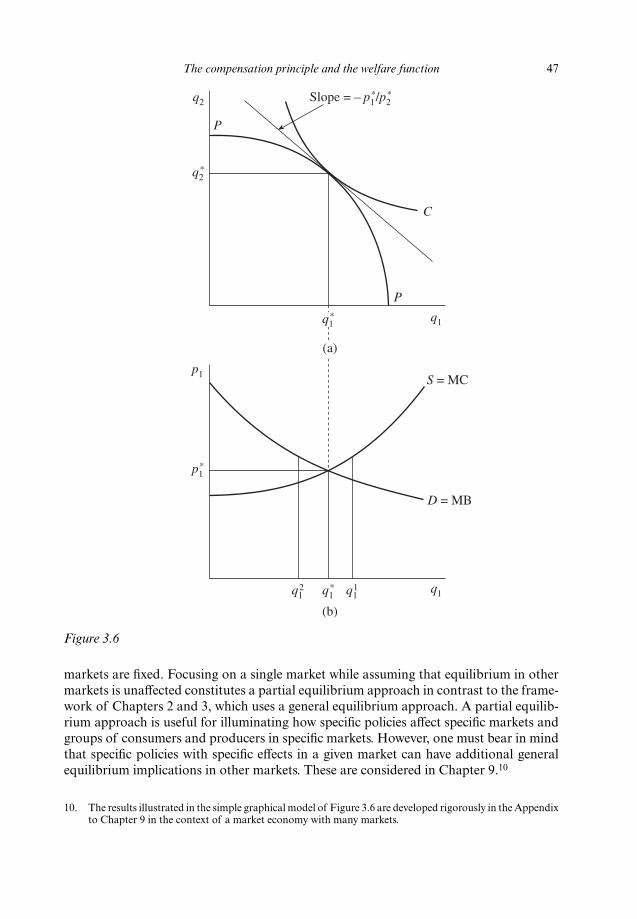
markets are fixed. Focusing on a single market while assuming that equilibrium in othermarkets is unaffected constitutes a partial equilibrium approach in contrast to the frame-work of Chapters 2 and 3, which uses a general equilibrium approach. A partial equilib-rium approach is useful for illuminating how specific policies affect specific markets andgroups of consumers and producers in specific markets. However, one must bear in mindthat specific policies with specific effects in a given market can have additional generalequilibrium implications in other markets. These are considered in Chapter 9.10


10. The results illustrated in the simple graphical model of Figure 3.6 are developed rigorously in the Appendixto Chapter 9 in the context of a market economy with many markets.

Figure 3.6

q1q12

q2

D = MB

q2*

p1 S = MC

p1*

q11q1

*

q1q1*

(a)

(b)

Slope = – p1*/p2

*

P

P

C

3.7 SUMMARY

This chapter has focused on the compensation principle and the social welfare functionas devices to aid policy-makers in using resources optimally. The compensation principlestates that state B is preferred to state A if, in making the move from state A to state B,the gainers can compensate the losers such that everyone could be made better off – thatis, if the WTP of the gainers exceeds the WTA of the losers. The principle is based onpotential rather than actual compensation. Some could actually be made worse off froma policy change, yet the change would be supported if the gainers could have compensatedthe losers so that everyone could have been better off. Because the principle is based onpotential rather than actual gains, two problems arise: the reversal paradox and theintransitivity problem. However, even though the criterion is based on potential gains,these problems can arise only if no first-best bundle is considered.

The concept of a utility possibility curve was introduced, and a parallel was drawnbetween the utility possibilities approach to welfare economics versus that based on pro-duction possibility frontiers and Scitovsky indifference curves. The notion of a potentialwelfare criterion was introduced. If this criterion is adhered to by policy-makers, all pos-sible bundles of goods have to be considered together with all possible distributions ofthese bundles. Such an approach is usually not empirically practical (although it is con-sidered further in Section 8.3).

Because the compensation principle cannot rank first-best bundles, the concept of awelfare function was introduced. If such a function were available and agreed upon, theoptimum organization could be obtained. But because agreement on such a functioncannot be reached, the compensation principle is apparently the most widely applicable,yet also empirically practical, criterion. However, one of the problems with the principleis that it is based on potential rather than actual gains. Thus, in any policy context, thepayment of compensation is a matter that must be decided by policy-makers endowedwith the authority to determine income distributional issues.


2. Pareto optimality and the Pareto criterion...principle and the concept of Pareto optimality. This...

Documents

Transcript of 2. Pareto optimality and the Pareto criterion...principle and the concept of Pareto optimality. This...