1

Efficacy of Lender of Last Resort, Access to Central Bank

Money and the Default Rate: France 1826-1913*

Vincent Bignon♦♦♦♦ Clemens Jobst◊◊◊◊

Banque de France Oesterreichische Nationalbank

Abstract

This paper measures whether a wider set of assets and counterparties eligible to central bank

refinancing makes lending of last resort more effective in avoiding defaults of firms. The data

includes default rates in 86 French districts each year between 1826 and 1913. The setup

allows identifying this effect independently of other aspect of Bagehot’s rule to lend freely

against good collateral. We exploit variation in the occurrence of a negative productivity

shock on the agricultural sector as an instrument for central bank money demand of the

industrial and service sectors. We then show that an easier access to central bank money in

terms of less restriction to eligible agents and assets reduces substantially the default rate. We

exclude that this policy succeeded because the central bank acts as a bad bank.

J.E.L. code: E32, E44, E51, E58, N14, N54 Keywords: credit easing, eligiblity rules, collateral, default rate, phylloxera, Bagehot.

* We thank Olivier Armantier, Jean Barthélémy, Régis Breton, Eve Caroli, Martin Eichenbaum, Christian Hellwig, Philip Hoffman, Antoine Martin, Kris Mitchener, Christian Pfister, Stefano Ugolini, François Velde, Jean Tirole, Eugene White and participants of the 2012 Norges Bank workshop “Writing Central Banks History” in Geneva and of the 2012 Economic History Association meeting in Vancouver for discussions, advice and comments. We are grateful to Claudine Bignon and Charlotte Coutand for their expert help with some of the data collection. The views expressed herein do not necessarily reflect those of the Banque de France, the Oesterreichische Nationalbank or the Eurosystem. Remaining errors are ours. ♦♦♦♦ Banque de France, Monetary Policy Research Division; DGEI-DEMFI-POMONE 041-1422, 31 rue Croix des Petits Champs, 75049 Paris Cedex 01, France. Email : vincent.bignon@banque-france.fr ◊◊◊◊ Oesterreichische Nationalbank; Otto-Wagner-Platz 3; 1090 Vienna (PO Box 61, 1011 Vienna), Austria Email : Clemens.Jobst@oenb.at

2

1. Introduction

Monetary policy is normally thought of as adjusting the nominal interest rate level or the quantity of

money. At the same time, the implementation of monetary policy decisions - while technically important -

is considered the domain of the front office and risk managers and gets little attention by academic

economists or the general public. In periods of financial stress, however, operational aspects can move to

the forefront, in particular the questions of who can get refinancing at the central bank and what are the

assets that the central bank is willing to buy or willing to lend against (Bindseil 2009, Chailloux et al. 2008).

Since 2007 and in particular after policy rates had reached levels where they could no longer decline any

significantly further, the interest of policy makers at the central banks of the major industrial countries has

to a significant extent shifted towards the choice of eligible counterparties and assets eligible for

refinancing (Borio and Disyatat 2009).

This paper aims to assess the effects of changes in eligibility on the performance of the real

economy. We measure whether the default rate of firms is impacted by the choice of the central bank to

increase the spectrum of agents and assets it accepts at its refinancing facilities. Is there some economic

loss triggered by the decision of a central bank to restrict itself to deal only with debt securities of some

issuers? Or by restricting the access to central bank money to a handful of bankers or only to some

selected credit institutions? Is there any economic improvement if the CB chooses to deal with the whole

class of safe debt securities? This is especially interesting since some argue that the central bank asset

holdings must be restricted to government debt only.

This evaluation is done using the eligibility rules of the French central bank and its impact on a

panel of local default rates in the 19th century. The reasons to go for a historic example are twofold. First,

central banks like continuity and big adjustments in eligibility rules are rare. Second, the identification of

the effects of being eligible vs. not being eligible is difficult empirically. Eligibility is often tied to

economic criteria (e.g. being a bank, having a certain rating) and is thus potentially endogenous to the

economic effects that should be assessed. Changes in eligibility rules in turn are often the result of

financial stress and thus again linked to the economic outcome we would like to analyze. In the case of the

19th century French central bank, like for many other central banks of time, however, eligibility was not

only based on economic but also geographic conditions, which are arguably exogenous. Richardson and

3

Troost (2009) used a similar identification strategy, when they looked at banks located in the same state

but on the two sides of the frontier between the Federal Reserve districts of Atlanta and St. Louis when

comparing the effects of the different monetary policies practiced by the two regional Feds. The present

paper looks at a uniform monetary policy but differences in eligibility.

The answer is that eligibility did matter. When an income shock hurt a district with broader access

to the central bank refinancing facilities, the default rate increased less than in districts in which the central

banks operated fewer facilities. There is considerable evidence that the positive effect of the Banque de

France came without costs – the central bank apparently only provided liquidity to agents that ultimately

turned out to be solvent.

An important advantage of our paper, compared to the existing empirical literature is that we can

rule out the endogeneity of the income shock to the central bank (anticipated) actions. To that end, we

follow the empirical strategy of Carlson, Mitchener and Richardson (2011) and study the consequence on

the industry and the services of the spread of an agricultural disease that triggered a major shock on the

local default rates. The shock we study is unrelated to any policy of the central bank before the crisis.

Because the central bank was prohibited by law from refinancing agriculture, we can rule out that when

taking decisions prior to the crisis, agents were anticipating the (future) relief provided by the central bank,

leading to moral hazard, increased risk taking and ex-ante increase in the default rate, thus provoking the

financial crisis in the first place. Furthermore no deposit insurance was operating, thus limiting the scope

for the application of Kareken and Wallace (1978) result of crisis driven by the actions of the public

authority. . Given that we find that extending eligibility helps the Banque de France to mitigate an

important part of the indirect consequences of the shock, our paper shows that the classical doctrine of

the lender of last resort (lend freely against good collateral) may usefully be complemented by adding

“using the broadest possible eligibility rule”.

Eligibility is a subject of high relevance. In the recent financial crisis eligibility has become a key

policy instrument on both sides of the Atlantic. Before 2007 the traditionally restrictive Fed had operated

with a very small number of counterparties, some twenty primary dealers, accepting only treasuries as

4

collateral. 1 In response to the tensions in financial markets the Fed decided to broaden access significantly

in 2008, both by creating new facilities for a much larger group of counterparties as well as by accepting a

significantly larger set of assets as collateral in lending operations (Cechetti 2009). For historical reasons

the Eurosystem had from the beginning of the single monetary policy in 1999 operated with a large

number of counterparties and a broad definition of eligible collateral that includes not only public and

private securities but also non-marketable assets like credit claims (Chailloux et al. 2008). Nevertheless,

during the crisis the Eurosystem considered it several times necessary to further enlarge the collateral pool

(ECB 2009, 2011). Both the Fed and the Eurosystem implemented these measures not as substitutes but

rather as complements to the more traditional interest rate policy, as policy makers feared that changes in

the interest rate alone would not be transmitted to the real economy because of stress in interbank

markets and market failure in financial markets more generally.

Our results complement the recent findings of empirical evaluation of credit easing programs. We

document that the increase in the variety of both assets and agents that were eligible to central bank

refinancing facilities helped mitigate the increase in the default rate caused by a massive income shock.

Our result is consistent with the finding by Krishnamurthy and Vissing-Mortensen (2011) that the first

round of the Fed’s large scale asset purchase programs (LSAPs) in the Fall 2008 that included purchases

of private assets – had a bigger impact on default risk than other LSAPs that involved only the buying of

Treasury debts. This result is also in line with the argument in Quinn and Roberds (2012). In their paper

they show that the swift reaction of the Bank of Amsterdam to the panic of 1763 that decided to broaden

the eligible collateral was decisive in avoiding the failures of key financial intermediaries. Recently

economists have started to wonder what the optimal credit policy of the central bank may be, i.e. whether

the central bank should pursue an active management of the assets side of its balance sheet (Woodford,

2012). This paper contributes to this literature by measuring whether the default rate of firms is impacted

by the increase of the spectrum of assets accepted by the central bank, holding constant the quality of the

eligible assets. 2 We confine our attention to whether increasing the eligibility of assets and agents to the

1 This is true for open market operations. The Fed’s discount window allows obtaining central bank refinancing for a much larger group of banks and against significantly wider range of collateral. However, due to stigma the discount window failed to serve its role for providing liquidity under stress (Armentier et al. 2011). 2 So far the theoretical literature has mainly discussed the issue of whether central bank should accept non-risky assets along with riskier assets (see Curdia and Woodford, 2011; Gertler and Karadi, 2012, Farmer, 2012). Williamson (2012) has a different focus. He argues that financial crises are bestl mitigated using open-market

5

operations of the central bank – both of them with (very) low credit risk – may improve the economic

outcome.

Our empirical exercise also contributes to the debate on the optimal form of liquidity provision in

periods of financial stress.3 Some authors have argued that central banks should only care about the

aggregate liquidity supply, leaving the distribution of liquidity to the market (Goodfriend, King 1988,

Bordo 1990, Schwartz 1992). Other authors like Repullo (2000) have argued that the same information

asymmetries that justify the existence of banks in the first place also render their loan portfolios illiquid

and might lead the interbank market to fail in periods of financial stress. During financial panics healthy

banks may also be tempted to manipulate their lending behavior for strategic purposes (Acharya, Gromb

and Yorulmazer, 2012). In all these cases it might be preferable to offer each and every bank direct access

to the central bank (Calomiris 1994, Flannery 1996, Freixas et al. 2000).

While it is clear that the limitations and motivations for the Banque de France then and central

banks today differ in many important respects, the economy we analyze in our paper has a number of

interesting features that makes it comparable in some respect with the current set up in which non-

conventional measures are implemented. First, the Banque de France operated with standing facilities, i.e.

it fully accommodated liquidity demand at the set interest rate and given the fulfillment of quality

requirements. This is very similar to the current framework of the Eurosystem operating with a fixed rate

full allotment policy. Second, being eligible or not was the main distinctive feature of agents (and assets)

while otherwise a single interest rate and uniform rules for the implementation of monetary policy applied

for the entire French territory. This is similar to the current understanding of a level playing field, where

central banks should not discriminate between counterparties as soon as they are eligible for central bank

operations. Finally, fiscal policy was passive in 19th century France, not smoothing out the type of regional

income shocks we examine at through by any interregional transfers. Again, the parallels to the limited

fiscal federalism in the Euro area are evident.

operations with Treasuries only. In a model with perfectly competitive banks, the purchase of private assets by the central bank does not impact the equilibrium prices or quantities, though it may redistribute wealth. 3 Inspired by the specific features of the operational framework of the US Fed, the debate has been framed in terms of discount window lending vs. open market operations. Its conclusion however can also be rephrased under the more general heading of eligibility.

6

The paper is organized as follows. Section 2 gives an outline of the argument and the design of the

empirical exercise. Sections 3 to 4 then provide the historical background of central bank refinancing in

more detail. Section 3 starts by explaining the rules for access to the Banque de France during the 19th

century while section 4 gives an overview of the evolution of central bank access in 19th century France.

Section 5 presents the extensive effort of data collection. Based on archives and published documents we

have assembled a dataset on the year-by-year evolution of the default rate, our measure for the effects of

liquidity shocks, as well as on the banking sector and the central bank for each of 86 French districts

(départements) between 1826 and 1913. Section 6 presents the empirical framework that we estimate. In

section 7 we discuss the productivity shock we study and demonstrate that broadening eligibility of agents

and assets to the Banque de France did in fact help mitigate the adverse liquidity shock. Section 8

concludes.

2. Does eligibility matters for the implementation of central bank monetary policy?

2.1. Conceptual framework

Central bank money is usually obtained by private agents against some asset. Two types of

transactions have usually been used: a loan against collateral or an outright purchase of some debt security.

In this paper an asset is defined as eligible at the central bank if the central bank trades it against

banknotes or CB reserves. In history the types of assets that have been accepted at the central bank have

varied hugely. In the U.S. before 2007 the variety was de facto limited since open-market operations were

implemented using the Federal government debt while the discount windows was seldom used. During

the 1920s, however, most of the CB transactions were made at the discount window using bills of

exchanges. The set of assets eligible was then much broader as bills could be issued by all private agents

and varied considerably in quality. As mentioned above, in the Eurosystem the variety of assets that can

be pledged as collateral is very broad and includes both government and private securities – sometimes

even if they are not listed. This was also a feature of 19th century European central banking practice.

Discounting implied that the variety of debt contracts that the central bank screened, bought, monitored

and cashed in was especially large.

For each existing asset, eligibility results from a binary decision by the central bank to accept it or

not in trade against its money. A number of criteria can be used to decide on eligibility. For example it is

7

customary for central bank to usually trade money against debt securities but not against variable income

securities. It is also customary for the central bank to screen the quality of the assets and accept only the

very safe ones. But this does not exhaust the criteria defining eligibility at the central bank. Within the

class of safe debt securities, the central bank can further choose to discriminate according to the sector of

the issuer, to its identity or legal status, or even to its address. Each of these choices contributes to

determine the share of eligible assets among the set of all assets. For example in a world with 10 assets

differing by riskiness and sectors, the proportion of asset eligible may vary between 10% and 100%,

depending on the eligibility decision by the central bank for each of those ten assets.

The choice of which assets are eligible impacts the cost of obtaining central bank money when

trading on the financial market is complicated by some imperfection. In an economy with perfectly

competitive markets, the absence of frictions makes irrelevant the choice of the variety of assets that the

central bank purchases against the money it creates since an agent holding a non-eligible asset can trade it

without cost against an eligible asset: Initial holdings do not impact on the situation of agents.

But when trading is complicated by some friction, an agent without an eligible asset but in need of

central bank money has to pay an intermediary that will sell him either an eligible asset or some central

bank money. A profit-maximizing intermediary operating with positive costs will charge a positive price to

the agents in need of central bank money. This generates a transaction cost that must be added to the

interest rate paid by the agent to trade its (non-eligible) asset against the central bank money. This has two

consequences. First in situation of high demand for CB money a very restricted set of eligible bonds

increases the price of those bonds and hence subsidize implicitly the issuers and/or holders of those

bonds. Secondly broadening eligibility impacts the effective interest rate –defined as the sum of the CB

interest rate and the transaction cost of obtaining the eligible asset– paid for central bank money.4

A number of mechanisms may explain why a restricted policy of eligibility may impact negatively

the default rate. Harsh penalty in case of default and a big enough aggregate (negative) shock may trigger a

substantial increase in the demand for eligible assets and hence of the effective price of accessing

monetary assets. This could be the case in situation in which the working of the financial (interbank)

4 This reasoning can be rephrased in terms of eligible agents, i.e. to the class of agents that enjoy direct access to the central bank. If only some part of the population has access to refinancing operations, those agents will act as intermediary in providing central bank money to the other part of the population –possibly against some collateral.

8

market is impaired by adverse selection and difficulty to signal its true credit risk (Acharya et al. 2012;

Heider, Hoerova and Holthausen, 2009). The relative scarcity of eligible assets to non-eligible assets may

explain interest volatility on the secured money market (Heider and Hoerova, 2009). In any of those cases,

the payment for the service of the intermediary consumes real resources that may force some agents to

default on the repayment of their debt not because of insolvency but because of the cost of accessing the

means of payment has temporarily increased. It is then possible to observe that a broadening of the

eligibility rules of the central bank reduce the transaction cost to access central bank money, thus reducing

the odds of default.

Our goal is to determine whether variations of the proportion of eligible assets in a given class of

debt contract had an impact on the variation of the default rate when the economy is hit by some (big-

enough) income shock. We estimate this relation using a difference-in-difference approach and pay special

attention to the (potential) endogeneity of the eligibility choice to the income choice. In their response to

the 2007/8 crisis, central banks have broaden eligibility to include assets issued by some distressed agents

or sectors. Some discussed those steps arguing that they aimed at helping a sector for a negative real

shock, which is usually not considered a task of monetary policy (but rather of fiscal policy). Some further

argued that this encouraged moral hazard. This leads some scholars to argue in favour of restricting the set

of eligible assets. We however remark that those changes were endogenous to the shock and hence that

drawing inference on those events to determine eligibility policy may be worth further discussion. In this

paper we study an episode in which the decisions on eligibility were unrelated to the sectoral productivity

shock and the central bank did not take any step to smooth its impact on the sector that were hit. The

next subsection describes our empirical design.

2.2. The empirical design

Our argument is that the existence of a positive (transaction) cost to access the central bank money

may force some agents to default despite them being solvent. The proper identification of this relation

requires a specific empirical design. The rest of this section describes our empirical design to test this

(negative) relation between the eligibility to central bank refinancing and the default rate.

9

The main challenge in evaluating the benefits of broadened eligibility to central bank facilities on

the default rate is empirical. A proper assessment requires the identification of a measure for the impact of

the central bank on economic activity and of a shock that increased liquidity demand by the private agents.

The shock must significantly increase liquidity demand by the private agents and hence have a direct

impact on the default rate. It also requires the existence of two well defined groups, one eligible for central

bank refinancing and the other that is not, and those groups must be set exogenously and independently

of the liquidity shock analyzed.

A typical shock that central banks address and that directly impact agents’ liquidity is a financial

crisis. Unfortunately, financial crises are ill-suited for the following reasons. First central banks being the

bank of banks tend to alter the rules of eligibility following financial shock in order to provide help to the

financial sector. This means that with a financial crisis, it cannot be excluded that eligibility is endogenous

to the shock, and hence the empirical exercise is likely to be biased finding a positive effect of eligibility on

the default rate. Second, agents’ actions may be endogenous to the central bank action and may lead them

to take excessive risk and hence trigger a financial crisis. The period we study does not have any deposit

insurance scheme but the central bank acted as a lender of last resort, and hence may have lead to moral

hazard behavior. Third, another classic problem in the study of financial crises is that it cannot be

excluded that the central bank deviated from the classical lender of last resort doctrine (lend only against

good collateral) and chose to refinance insolvent firms. If this were the case, the central bank would have

acted as a bad bank. Together endogeneity, moral hazard and the taking-over of losses by the central bank

after the crisis might bias the default rate upwards before the crisis and downwards after, leading to the

wrong conclusion that the eligibility rule had the effect of mitigating the increase in the default rate.

To avoid those issues of reverse causality and omitted variables, we study the consequence of a real

shock to the agricultural sector –phylloxera- a disease of vines.5 Phylloxera has several important

advantages. (i) The size of the shock was most likely big enough to have a discernable impact on the other

sectors of the economy. (ii) The phylloxera was a real shock to the productive capacity of the agricultural

5 Phylloxera is an insect that attacks the roots of vines and leads to a rapid loss in production. It arrived on French territory in 1863 and no effective treatment was available before 1890, hence its spread was exogenous to farmers’ actions. There is no potential reverse causality as its spread was not influenced by the agents’ default decisions. This shock has been used to assess the effects of a large productivity shock in other papers. Banerjee, Duflo, Postel-vinay and Watts (2010) shows that the bug triggered significant long-run health impact while Bignon, Caroli and Galbiati (2011) shows that it contributed to increase the criminal activity.

10

sector, and hence our result cannot be driven by changes in expectations alone. (iii) The shock hit a sector

that had no access to the facilities supplied by the central bank, thus ruling out that our results come from

a differential implementation of monetary policy across the various districts. (iv) The shock was

independent of the action of any of the agents of the economy, thus ruling out that their past actions

caused the shock. (v) To banks, services and industry, the shock was as close as possible to a pure

temporary (income) shock. (vi) The shock spread gradually over the territory.

We are interested in knowing whether the central bank helped to mitigate the consequence of this

agricultural productivity shock on banks, services and industry. Phylloxera also constituted a liquidity

shock on the banking sector. Because it was exogenous to the actions of the banks and because it must

have prompted withdrawals by distressed farmers, it acts as an aggregate liquidity shock on the local

banking system. The size of the shock on the French economy was also noticeable, explaining one third of

the drop in the production of a sector whose size represented 7% of the GDP in the year preceding the

arrival of the disease in France.

Two types of financial institutions could have helped the regional economies to smooth the

consequences of this shock: either deposit banks with branches operated in various regions of the French

territory or the central bank. Multi-branches deposit banks could have helped if they redistributed liquidity

across the regions by granting loans to agents in distressed places using the deposits of those agents in

locations free of the disease. Another possibility was the central bank issuing banknotes to finance

distressed agents in plagued regions. Both types of banks used the same loan technology, i.e. they

discounted short-term bills. An important difference was that the opportunity cost of their resources

differed because the opportunity cost of the central bank must have been much smaller. Holmstrom and

Tirole (1998) highlighted that the central bank should have been especially effective in this type of

situation when the size of the aggregate was large enough. In our paper, the issue of whether the national

deposit banks or the central banks were more effective in smoothing out the consequence of this shock is

an empirical question. One specification will control for the (potential) involvement of both deposit banks

and the central bank.

11

We want to be sure that we have identified the impact of differences in eligibility on differences in

the default rate. To this end we study a panel of French districts (each being equivalent in size to a US

county) that did not differ in terms of monetary policy except for the eligibility dimension, i.e. some

benefited from an easier access to the central bank facility than others. We can easily rule out that our

results are explained by interest rate variations. The law required the interest rate to be the same over the

whole French territory and the central bank had no right to apply different prices according to the quality

of assets or counterparties, though it could deny access to those that did not match a minimal quality

threshold. The central bank did not alter its commitment to refinance any solvent agents during the whole

period, thus allowing to exclude that our result are driven by changes in the CB forward guidance

(Eggerston and Woodford, 2003). Moreover the statutes of the central bank enacted that anyone fulfilling

the quality criteria was potentially eligible to central bank refinancing, except for constraints imposed by

the payment technology of the time.

Our strategy to identify the impact of eligibility on the default rate uses a peculiarity of the legal

characteristics of the bills of exchanges, which were the main type of assets used in the financing of the

French economy during that period. The law required the owner of a bill of exchange to collect the

payment of the bill at the debtor’s door. Financial intermediaries that held bills to maturity therefore had

to set up an organization to collect payment within a given geographic area. The possibility to buy and

hold bills to maturity was constrained by the size of this area. Because the technology did not change

significantly during the whole century in terms of the collection of payments, the extension of the assets

eligible for discounting was tied to the set up of local collection facilities, most importantly in the form of

new branches. It follows that the variety of bills discountable at a bank was conditional on the number of

branches it operated on the territory. Notice that the central bank was forced to hold bills to maturity

while other banks could always ask for the rediscounting of part of their holdings.

The extension of the size of the branch network of the central bank had two consequences in terms

of increased eligibility. First it increases the number of agents eligible to refinancing operations because it

allowed any trader residing in the city in which the central bank operated a branch to open a bank account

and hence to ask for rediscounting. Second it was an extension of the number of assets eligible to

refinancing. The opening of a branch in city X allowed those living in other cities with an account at the

12

central bank to ask for the rediscounting of bills payable in city X. The geographical extension of the

network corresponded to an increase in eligible counterparties, as more and more places in which bills of

exchange were payable became part of the business of central banking.

This peculiar design of central bank access allows comparing the impact of liquidity shocks for

regions that only differed with respect to their access to the central bank.6 Section 4 discusses the reason

for the extension of the network and argues that it was driven by a combination of political and economic

factors that were unrelated to economic crises or specific liquidity shocks and can thus be treated as

exogenous to the question at hand. Therefore, if a given liquidity shock had a smaller impact in districts

served by BdF this could be attributed to the chance of having direct central bank access.7 Sections 3 and

4 present the eligibility rules and the motive to broaden them. Section 5 describes the empirical

framework, section 6 presents the data and results are discussed in section 7.

3. Eligibility rules in 19th century central bank operations

During the entire 19th century the bill of exchange was the main instrument used by agents to

obtain refinancing from the central bank. The operation involved agents in need for cash asking for the

escompte (discount) of a bill by the Banque de France, which meant that the bank bought the claim at its

nominal value deduction made of a discount that was determined by the residual maturity of the bill and

the discount rate. By discounting, i.e. buying the bill, the central bank became the payee and it would be

paid at due date by the drawee named on the bill at an address that was also specified on the bill. The

discount rate was set by the bank and applied, according to the 1808 decree that organized the statute of

the bank, indiscriminately in any of the places where the bank had an office. This provision forbade the

bank to adjust the discount rate to local conditions. Alternatively, central bank money could also be

obtained through collateralized lending called avances sur métaux precieux ou titres, i.e. a loan on collateral,

6 There is of course the possibility to obtain central bank liquidity indirectly. In case the central bank was not present in some district, firms located in this district and hit by a liquidity shock on the aggregate district level could have relied on intermediaries or firms active outside the district. However, when the central bank extended the extent of its monetary policy operations to a new district it must have reduced the transaction cost of arranging the furniture of liquidity – compared to the previous situation with intermediaries between the central bank and the agents. 7 We would also like to exclude that different outcomes can be attributed to other aspects of central bank policy, like e.g. quantitative restrictions in refinancing or the application of different interest rates in different regions. Those conditions are fulfilled for the 19th century Banque de France.

13

either gold or silver or securities.8 During the period under study, discounting was by far a much more

important activity than collateralized lending. Discounting represented on average 91% of central bank

operations during the period 1826-1913.

The preference for discounting was to a large extent due to the safety of the asset. Bills were

favoured because the law carefully organized the transfer of the ownership of bills. Each transfer of a bill

(i.e. each act of discounting) left the previous owners with a joint liability vis-à-vis the purchaser of the bill

(the discounter). Indeed each purchaser of a bill signed the bill, which was an acknowledgement of his

commitment to pay the bill in case of default by the drawee. The exercise of this clause of joint-liability

clause was quick and relatively easy. It required only the protestation of the bill, i.e. the ascertainment of

the default by a bailiff, a notary or two witnesses at the moment the bills fell due. For example the simple

absence of the payer in due time at the scheduled place sufficed for the payee to protest the bill, which

instantly allowed him to invoke the guarantee of the last endorser, asking him to pay in lieu of the initial

payer. If this person also failed, and if the bill was endorsed by another person, the joint liability clause

again applied, and so on up to the drawer of the bill.9 The incentives created by the joint liability must

have lead discounters to carefully scrutinize the quality of the bills they decided to guarantee, i.e. to refuse

the discounting of the bill whenever they doubted the solvency of the payer. 10

Access to the facilities for discount and advances was both broad and restricted at the same time. In

contrast to nowadays, everybody fulfilling some minimum criteria could obtain funds from the Banque de

France (Cameron, 1967, p. 121). The main formal restriction was the requirement for any agent to open

an account at the Banque and hence to have an address in a town where the Banque de France operated a

branch.11 Between 1817 and 1835 that meant living in Paris. The rule didn’t change over the century. But

after 1836 when the Banque de France started to open branches outside Paris, the number of people who

8 France was on a metallic standard – bimetallic until 1873 and de facto (if not de jure) only gold thereafter. The cover rule required a certain percentage of the banknotes in circulation to be covered by holdings of precious metals (see Ugolini 2012). Note that the BdF suspended convertibility only during the 1848 revolution and the Franco-Prussian War and that after the 1870s metallic reserves sufficiently large so that the cover rule never constrained the issue of additional banknotes (Bignon 2011). 9 Dalloz (1830, p. 128). 10 We are not aware of any study on the diffusion of bills among traders, and on the degree to which its use spread out in local communities, although the increase of the ratio of circulating bills to GDP may indicate the broadening of the number of discounters. Roulleau (1913) documented a declining average value of the circulating bills, which he interpreted as a greater diffusion of the bills as a tool for short-term finance. 11 Exceptions were made for important receivers-general in the provinces (Gille 1959 p 86).

14

could access its services increased significantly.12 By 1913 the inhabitants of 218 towns had the possibility

to open an account at the BdF and thereby access to the discount and the Lombard facility (see figure 1).

In 1913 86,200 persons had taken this opportunity (Lescure, 2003, p. 139). The eligibility of counterparties

depended thus to a large extent on a geographic criterion.

The same was true for which bills were considered eligible. A bill was a claim whose payment had

to be collected at the payer’s doors. Because bills were held to maturity, the central bank was only willing

to accept bills payable in places in which it could actually claim the payment without the need for another

intermediary. This required either the payee to keep an account with the Banque de France or an officer of

the bank had to be sent and collect the payment. In both cases the bank had to be physically present. As

long as the only office of the bank was in Paris, that meant that that only bills payable in Paris were

discounted by the bank.13 While other eligibility criteria of bills were gradually loosened, particularly in the

later decades of the 19th century, the domiciliation requirement for bills to be payable in a city were the

Banque de France was represented was maintained.14 Indeed the payment technology of bills did not

change over the 19th century, nor did the domiciliation criterion. Hence opening a branch in a city not

only allowed more agents to become a counterparty of the bank but also made more bills eligible, thereby

extending the proportion of assets – among the whole set of existing assets – against which central bank

money could be obtained. By 1913 almost 600 cities and towns counted as places banquables.

12 The extension of the network of branches by the Banque de France followed a first attempt made during the Napoleonic period (see Pruneaux, 2009 for details). 13 This constraint was further reinforced by the government when it enacted in 1808 that the bank was only allowed to discount bills payable in Paris, or later a town where the Bank was represented (a bankable place, i.e. a branch or a designated town in which the bank send its collectors to cash in the bills). 14 At the beginning of the Banque de France operation, bills also had to fulfil other criteria concerning a minimum and a maximum maturity, a minimum amount and the number and quality of signatures. According to Article IX of the Statuts fondamentaux of 1808 bills had to have a term of at most three months and carry the signatures of at least three merchants or bankers. The requirement of three signatures implied that a commercial bill would have to be discounted already once before becoming eligible to the BdF, i.e. de facto to be held by a banker or merchant. Together with the minimum amount this rule restricted credit to a small group of bankers and merchants at least in the first decades of the bank’s operation. Over the century eligibility requirements were gradually loosened. From 1833 onwards, e.g. the third signature normally required could be replaced by pledging government debt (Cameron, 1967, p. 123), after 1869 all securities eligible for advances (Décret of 13/01/1869 and article 3 of the law of 30/6/1840). In 1898 certificates for warehoused agricultural produce (warrants) were admitted for discount (Ramon 1929 p. 416). The minimum amount for bills was gradually lowered from XX francs in 1800 to 5 francs in 1898 (Ramon 1929 p. 416). A similar loosening can be observed for advances on collateral, where also the borrowing limit was lowered over time and the range of eligible collateral extended from only gold and silver at the beginning to include securities issued by the central government, then by the city of Paris, government-guaranteed railroads, mortgage-backed bonds, local governments etc. by the end of the 19th century (Ramon 1929 pp. 277, 311, 403).

15

Figure 1: The number of branches operated by the bank of France, 1826-1913

Source: Jobst (2010)

Even though bills were by construction relatively safe assets, another consequence of the outright

purchase of bills was the need to monitor default risk if the discounted bills ended up being unpaid. As a

privately owned company traded on the stock exchange, the Banque de France had a keen interest to

minimize its exposure to default so as to protect profitability. It was also by law required only to discount

bills that were endorsed by at least three persons who were notoriously solvent.15 In order to ascertain the

quality of bills bought, the management delegated the screening of the solvency of its counterparties to

discount committees that decided the acceptance of bills presented. The discount committees typically

comprised persons nominated by some of the shareholders of the bank and some of its regents.16 The

watchdog of the discount committee was the Portfolio committee – composed of board members of the

bank. It was in charge of examining the legality of the decisions of the discount committees, notably the

fulfilment of the clause that forbade the bank to lend to bankrupted agents.17 Finally any decision of the

bank was ultimately monitored by three shareholders (censeurs) in charge of overseeing the bank’s activities.

Elected by the shareholders the censeurs had to select the discount committee and approve the issue of

15 Article 11 of the Decree dated 01/16/1808 : “ La Banque, soit à Paris, soit dans les comptoirs et succursales, n’admet à l’escompte que des effets de commerce à ordre, timbrés et garantis par trois signatures au moins, notoirement solvables”. 16 This is true for the Paris office but also for each branch (see article 35 and 36 of the decree dated 09/08/1808). 17 Articles 58 and 59 of the Statutes, ibid.

050

100

150

200

0

50

100

150

200nu

mbe

r of

citi

es w

ith a

bra

nch

1820 1840 1860 1880 1900 1920year

Main and auxiliary branches Main branches

16

banknotes.18 Moreover a special body of employees –the inspection –monitored the activity of the branches

operated outside Paris.

To sum up this historical tour into 19th century central eligibility and collateral policy, the geographical

extension of the operation of the central bank meant that the number of eligible counterparties rose

significantly and that an increasing share of bills became acceptable for central bank rediscounting. This

peculiar design of central bank access allows comparing the impact of liquidity shocks for regions that

only differed with respect to their access to the central bank. The next section describes the gradual

extension of the branch network.

4. Rationales for and constraints on the development of the bank branches

Historians explain the development of branches by the Banque de France as the outcome of both

political and competitive pressures from merchants and political elites of the main French cities outside

Paris. Indeed, the bank did not possess a monopoly of banknotes issuance on the whole French territory.

The statutes of the bank granted it a monopoly of note issue only in Paris and in the cities in which it

maintained branches (Cameron, 1967, p. 126). Competitors could then lobby the government for the

opening of a bank of issue in cities in which the Banque de France had no branch. This provided the

government, politicians and local merchants with a strong argument either to convince the bank to open

branches in the provinces or to allow a competitor to enter in a city in which the Banque de France did

not operate a branch . After the Napoleonic period, which is outside of the scope of this study, four main

episodes in the history of the branches can be distinguished.19 All of them were clouded by political

interferences in the decision making process of the bank. Each was linked to the discussion and

negotiations on the renewal of the privilege of notes issuance.

The period between 1817 and 1848 was characterized by multiple banks of issue. Indeed following

the demise of the Empire in 1815, the Banque de France closed its regional branches, which had been set

up mainly for political reasons.20 The bank considered that branches were unprofitable and difficult to

manage and preferred to restrict its activity to Paris. The economic and political elites of the major French

18 Article 46 of the statutes, ibid. 19 The episodes of importance were the end of the 1830’s- beginning of the 1840’s, then the period of the Second Empire, the third took place during the 1870’s with the passing of the law on branches and the last period of opening was linked to the renewal of the privilege in 1897. 20 Plessis 1998 (1967), p. 83; Ramon 1929 p.123, 129-130.

17

commercial cities were unhappy with this situation and pushed for the creation of local banks of issue

(banques départementales), arguing that the cities known for hosting markets of regional importance needed

banks of issue to cater to their regional financial needs.

The local banks of issue were launched following an intense lobbying for the necessary royal

approval and the approval of the Banque de France, which was always consulted on the matter (Gille,

1970). Nine banks succeeded in securing the privilege and were thereby created, three in 1817 and 1818

and six more in the second half of the 1830s.21 Each enjoyed the monopoly of notes issue in the city

where it operated. After some initial hesitancy, the Banque de France considered this movement as a

threat to its business model.22 For example one of the two deputy governors of the Banque de France

argued in an executive meeting dated February 1836 that “Soon there will be nothing left of the monopoly

of the bank (…) If the bank does not wish to be completely disinherited in the départements [districts], it

must be hasten to take steps to occupy the cities of the second order, lacking cities first order, so that it

merits its title of Banque de France, and preserves, in view of the approaching renewal of its charter, a

facility which might otherwise be compromised”.23

Faced with mounting and increasingly fierce competition, the bank switched strategy and decided to

open new branches itself – first in Reims in 1836– and to lobby the government and legislature to make

the opening of new independent banks of issue more complicated. A law in 1840 tilted the balances

between monopoly vs. multiplicity of issuing banks decidedly in favour of the Banque de France. As a

result fifteen branches, each in a different city, were opened in the eight years that followed, while no new

independent local bank was founded. In 1848 the financial crisis and the revolution hastened the process

and in an emergency measure local issuing banks were merged with Banque de France. The era of local

issuing banks came to a close (Ramon, 1929, p. 230).24

The granting in 1848 of a de facto monopoly of banknotes issuance over the whole territory left

however the Bank still hesitant when it came to opening new branches, mainly for reasons of governance

21 Bordeaux (1818), Nantes (1818), Rouen (1819), Marseilles and Lyons (1835), Lille (1836), Le Havre (1837), Toulouse and Orléans (1838) Marseilles (1840). See Kindleberger (1993, p. 105-106). Gille (1970) described the birth and operation of four of those banks, Le Havre, Lille, Lyons, Marseilles and the demise of the project proposed by Dijon. Cameron (1967, p. 125) mentioned that the Banque de France impeded the creation of nine issuing banks. 22 Ramon 1929, p. 175-6; Cameron, 1967, p. 104, 123-7 23 Procès verbaux du Conseil general, vol. 20, fol. 220, 25 February 1836, cited in Cameron (1967, p. 104) 24 except for one short episode in 1860 with the incorporation of the Savoy and the coming of the bank of Savoy

18

of the local branch and risk management of the portfolio of a profit-maximizing institution. But the

competitive threat from the banking sector remained an important stimulus to pursue the opening of new

branches. During the twenty years of the second Empire (1852-1870), the Banque de France faced two

main challengers. First the Pereires brothers were very active in attempting to influence the emperor to

secure privilege for their own banking businesses (Cameron, 1961, p. 138-44). After trying to issue their

own interest-bearing banknotes in the 1850s, they attempted in 1860 to breach the note issuing monopoly

of the Banque de France by taking over the Bank of Savoy, which according to the treaty that

incorporated the territory of Savoy into France had retained its note issuing privilege. The outcome of this

intense fight was losing battles by the Pereires but an extended branching by the central bank.

By the 1860s, the profit and position of the Banque de France were threatened by the rise of

national deposit branch banks like the Crédit Lyonnais or the Société Générale. Relying on extended

branch networks those national deposit banks collected significant amounts of deposits that they

employed in the discount business. As they hardly ever rediscounted their bill portfolios at the Banque de

France, this development severely hit the core income generating business area of the bank (Lescure,

2003, p. 136-7). This brought about another reconsideration of the merits of branching as a generator of

additional discount business. The bank’s directors reacted by supporting smaller regional and local banks,

that refinanced their bill portfolios at the Banque de France, and by encouraging non-bank clients to use

the central bank lending facilities (Plessis 1985, Nishimura 1995 p. 547). As competition for good bills was

fiercest in the larger cities, establishing a presence in more remote places was a way to increase business.

However, except during the early 1850s, the opening of new branches followed an uneven

evolution. While a constant political pressure – lobbying from the local elites – and competitive threat

from banking persisted during the second half of the century, an important driver was the recurring

(re)negotiations with the government and Parliament on the occasion of the expiration and necessary

renewal of the statutes and of the monopoly rights granted therein. Every renewal of the privileges gave

rise to political demands to extend services both at existing branches and through the creation of new

branches. Besides 1840, renewal was granted in 1857, in 1897 and in 1911. In 1873 a law activated the

clause contained in a law passed in 1857 to force the Banque de France to operate at least one branch in

each district by the beginning of 1877 (Plessis, 1985, p. 199-201). The two decades spanning in the 1860s

19

and 1870s and the post-1897 years were then characterized by an intense activity of branching and it is fair

to say that the chronology fits well the political-financial nexus. Added to the external pressure came,

according to Lescure (2003), the ethos of a new generation of bank officials with a republican background

who came to dominate the bank in the 1880s striving for the decentralization, diversification and

extension of the bank’s operations. In these years the BdF not only expanded geographically, but

implemented significant simplifications in the access to its discount, Lombard and giro facilities (ibid p.

138). Being the bank of the general public, not only of the other banks, became the objective by the 1900s,

at least if we believe the public declarations of governor Pallain (1897-1920). In the end more and more

regions and cities enjoyed a direct access to central bank refinancing facilities. By 1879 there is at least one

branch per district and over the course of the century more and more districts benefited from more than

one branch (figure 2).

Figure 2: Number of districts with no, one, and more than one BdF branch offices

The history (timing) of the branch openings was thus the outcome of a bargain triggered by the

discussions on -or threats to- the monopoly of the note issue. The Banque de France was a profit

maximizing firm and not a single branch made losses during the period, except during the very first years

of operation. But the losses were not the result of poor management but of the huge costs of setting-up a

branch. In the 1890s the Bank estimated those costs to be about 160.000 Francs, and the annual operating

0

20

40

60

80

100

num

ber

of d

istr

icts

1820 1830 1840 1850 1860 1870 1880 1890 1900 1910 1920

year

without any BdF branch with one BdF branchwith more than one BdF branch Total

Source: Author's computation using Annual Report to the Shareholders of the Banque de France

20

costs at 36.000 Francs for a small branch (succursale), at a time when the hourly wage of a qualified blue

collar rarely exceeded 1 franc.25

A new branch was always opened with long-term concerns in mind – profitability, regional

economic development, political pressure – but never to address an acute crisis. Doing so would have

been potentially very costly – the BdF never closed a branch office once opened and so the long-term

viability of the office was primordial. The opening of a branch office typically required a lead time of one

year. Before the opening a new office the Bank sent an inspector on-site who would assess the likely

volume and risk characteristics of the local demand for (re)discounting.26 As soon as a positive decision

was taken, a building had to be found, a director and staff to be recruited and the members of the

committee that examined the bills submitted (comité de censure) be nominated. The sluggish process of

creating new branch offices thus makes for a fundamental difference with swift ad hoc extensions of the

eligibility to central bank facilities in the recent crisis.

This analysis leads us to discard a potential endogeneity between the income shock we study and

the decision by the central bank to open a branch office. Neither the timing of the opening, nor the

constraints faced by the bank in terms of branch opening fit with the spread of the phylloxera across

French vineyards. The high set-up cost of branches was a strong motivation for a profit-maximizing

central bank to avoid opening branches to mitigate temporary shocks. This is substantiated by the fact that

the bank never closed a branch. Finally the fact that the law prohibited the Banque de France to refinance

agriculture –and the strong aversion of the bank against risk taking in its discounting activity– are

additional arguments that the openings of branches were unrelated to the phylloxera.

5. Data

This paper assembles datasets with yearly observation on the number of defaults, firms, and

statistics on the monetary interventions at the district level between 1826 and 1913. We have recorded for

25 BdF archives collection of parliamentary papers concerning the “Renouvellement du privilège de la Banque de France 1892-1897” CD V 1892/1649. Hourly wage is from INSEE (1946, p. *222-3). 26 BdF archives 1069199101/30 “Transformations de bureaux auxiliaires en succursales (1895-1912), études préliminaires” and “Création de bureaux auxiliaires (1907-1912), études préliminaires”.

21

each year the number of branches of the two main national deposit banks, the Crédit Lyonnais and the

Société Générale and have merged those with demographic variables, wine statistics and the phylloxera.

5.1. The measure of defaults

In our empirical setting, default was especially costly and we may safely assume that everyone tried

to avoid its occurrence. Default involves the opening of a legal procedure during which debts were

ascertained and creditors had to settle the future of the firm (see below). The firm had to stop its activity

during this period to protect creditors from inappropriate seizure by acquaintance(s) of the defaulted. No

creditor could escape the procedure and hence the debt was in a standstill upon agreement among

creditors. The average duration of the procedure was one year, which implies that correlated illiquidity-

driven defaults may arise as a result. Anecdotal evidence abound that when payment incidents started, it

was difficult to prevent them because of the average duration of the procedure and the impossibility for

creditors to exit or avoid the procedure before its legal termination.

The number of defaults per district is known by counting the number of judicial procedures opened

during a year in a judicial court. This procedure was called faillite (failure). This judicial procedure existed

to allow the assessment by the various creditors of the financial and economic conditions of the firms.

The creditors were the ultimate decision-makers on the continuation or not of the activity of the defaulted

firm. They were assisted by a judge who as the record keeper of the events occurring during the procedure

and the comptroller of the legality of the decisions taken by the creditors. It was assisted by an agent – the

syndic – specialized in the screening of the assets and liabilities of the bankrupted firm. No creditor could

decide to opt out of the procedure before the end of the procedure except by renouncing to its claim.

The definition of a faillite in French law has a number of convenient features for the question at

hand. In particular, the opening of a faillite procedure was tied to illiquidity and not to insolvency.

According to both the law and the jurisprudence the role of the procedure consisted in protecting the

equality of the creditors when the debtor proved unable to pay one of its creditors. In this context a

procedure of faillite aimed at screening the value of the assets, in ascertaining the effectiveness of the

liabilities (so as to avoid some creditors to be spoilt by made-up claims) and in deciding on whether the

22

business must be discontinued (in which case the monetary value of the assets was shared between the

creditors) or whether the firm had to continue in operation.

In order to limit as much as possible anti-competitive or political interference into business, the law

strove to use a trigger for the faillite procedure that could not be easily manipulated by one of the parties

concerned. To this end it was decided that faillite procedure may be opened only following the recognition

of a default. Legal scholars were clear that the state of insolvency in itself could never be a motive to the

opening of a faillite procedure and that insolvency could only be the result of a proper screening of a firm

during such a procedure (Percerou, 1935).27 This reasoning had the implication that no judge could force

an insolvent – but liquid – firm to file for a faillite procedure. Default was harshly punished. If creditors

were not entirely reimbursed and they denied the debtor the right to restart the business, the defaulter was

deprived of his legal and commercial rights. When creditors decided to allow the continuation of the

business, and provided a debt restructuring was agreed upon, the defaulter did not recover his legal rights

before having completed the reimbursement.

As a result the number of faillite procedures opened during a year in a given district can be used as a

direct measure of the number of defaults. An additional convenient feature of the law was that not all

businesses or agents were allowed to file for faillite. Only traders (commerçants, i.e. those who sell goods or

services on the market for profit purposes) qualified for the procedure, while workers and other non-

traders were excluded as well as farmers.28 This comes in handy below, when we use an income shock to

the agricultural sector to assess the effects of central bank liquidity support. Also importantly, neither the

definition of faillite nor the scope of businesses to which the law applied changed during the 19th century.

27 Article 437 alinea 1 of the 1807 commercial code enacted that: « Any trader that cease paying is in a state of failure” (« Tout commerçant qui cesse ses paiements est en état de faillite »). The legal scholar Percerou (1935, p. 207-8) commented that « la faillite en France se constate par l’impossibilité de payer. Elle se distingue de la déconfiture des non-commercants (i.e. exercant une profession civile) ». Percerou added in paragraph 181 that « pour savoir si la faillite doit etre ouverte, on n’a pas à examiner si le commerçant est solvable ou non, mais uniquement si de fait il paye ou ne paye pas ». 28 Notice that this did not imply that payment obligation were not enforced with those agents but rather than frustrated creditors have to ask the debt repayment using another judicial procedure (Percerou, 1935, p. 207-8).

23

The yearly numbers on new defaults (faillites) were gathered in the National Archives for the 1820-1850

period and from the yearly Compte général de la justice civile et commerciale between 1850-1913.29

5.2. Wine and phylloxera

Data on wine production and phylloxera come from Galet (1957). A year before the phylloxera

aphid was first spotted in the Gard district in 1863, wine was produced in 79 out of the 89 French

districts.30 The share of wine in agricultural production was then greater than 15% in 40 districts. The only

non-wine producing districts were located in the Normandy and the North of France. All the others

produced at least some wine.

The shock of the phylloxera attack on the other sectors of the local economy may also vary

according to the share of wine in the district GDP. To this end we use Delafortrie and Morice (1959) to

compute the share in the local GDP of the wine production during the year just before the phylloxera

appeared. Galet (1957) gives no information on the presence of the phylloxera in two districts, the

Ardèche and the Creuse. They were therefore dropped from the regression analysis.

We have used data collected by Banerjee, Duflo, Postel Vinay and Watts (2010) on the years of

presence of the phylloxera in each district and on the variables of wine cultivation and wine production.

Phylloxerait measures the impact of the shock created by the bug on the economy of district i during year t.

Its size is the product of an indicator of the presence of the phylloxera in the district with the share of the

wine production in the local GDP in 1862. The time it took for the bug to spread into each district varied

across districts and time. Hence no single lag-structure can account for it. This uncertainty leads us to use

three alternative variables to measure the size of the shock induced by phylloxera. All variable are

weighted by the size of wine production in the district GDP in the pre-aphid year 1862.

The first variable is labelled “presence”. It is equal to the product of the share of wine in the 1862

GDP with an indicator – labelled “Galet” – of the presence of the phylloxera in the district. This indicator

is set to 1 in any year between the first year the aphid was spotted in the district and 1890 – which is the

29 The faillite procedure encompassed any type of trader (i.e. any independent business such as wholesaler, shopkeeper, trader, insurer, banker or manufacturer that regularly earn revenue from the selling of products and/or services) but no firms operated in the agricultural sector. 30 Three districts had to be dropped because some data was missing for them, leaving 86 districts in the sample.

24

year during which the cure to the disease was implemented. In any year before the aphid arrived in the

district and after the implementation of the treatment, we set this indicator to 0.

The second variable is labelled “shock”. It is the product of the share of wine in the 1862 GDP

with an indicator constructed by Banerjee et al. (2010). They define this indicator as equal to if two

conditions are fulfilled. First the aphid is present in the district (the indicator “Galet” is equal to 1) and

second wine production had fallen below its pre-phylloxera level (i.e. below the level it had reached during

the last year before Galet =1). This indicator is set to 0 if “Galet” is equal to 0 and after the

implementation of an effective treatment (i.e. after 1890). This variable takes into account the fact that it

took time for the aphid to destroy the vineyards, though no information is available on the spread of the

aphid within each district.

The third variable is labelled “weighted shock”. It is constructed by multiplying the variable

“shock” by the size of the loss of wine production caused by the phylloxera. Banerjee et al. (2010)

constructed it by comparing the actual level of production with the one reached during the last year before

the phylloxera was spotted in a district.

5.3. Other data

During the 19th century France was composed of about less than 90 districts whose size was on

average about the size of a U.S. county. Two main changes in frontier made the panel slightly unbalanced.

First, in 1860 France incorporated three new districts with the annexation of the Savoy. Second, the war

with Prussia in 1870 ended with the loss of two districts of Alsace and of half of the Meurthe district and

half of the Moselle district. The remaining parts of the last two districts were merged into a newly formed

district, Meurthe-et- Moselle. A remaining part of the district Haut-Rhin that stayed French is named

Territoire de Belfort. In the regressions the Territory of Belfort is merged with Haute Saone, as default

figures from Haute Saone refer also to Belfort.31

We have collected by hand the number of firms operated during a year in each district using the

statistics on the French business tax (patentes) paid by any business selling goods or services on the market.

This included (among others) shopkeepers but also wholesalers, various types of factories, craftsmen,

31 Bignon (2011) presents in details the corrections that had to be implemented to render the series consistent over time.

25

banking and insurance firms. The agricultural sector was exempted from its payment and hence farmers

were not counted among the firms. Data on population in each district were taken from Bignon, Caroli

and Galbiatti (2011).32

Statistics on the central bank activity were taken from the Annual Report to the General Assembly

of the Shareholders. A typical report indicated whether a branch of the bank was active or not during the

year of the report. It also provides with the volumes of bills of exchanges discounted during that year by

each particular branch.

6. Empirical framework

In this context we estimate three equations. First we verify that the default rates of the services and

the industry reacts positively to the spread of the disease weighted by the size of the shock. Second we

also verify that the central bank did increase its refinancing following the spread of the disease, therefore

verifying that hurt firms turn to the central bank to help them smooth the impact of the income shock.

Third we estimate whether variations in eligibility were associated with variations in the default rate when

the shock hurt the districts.

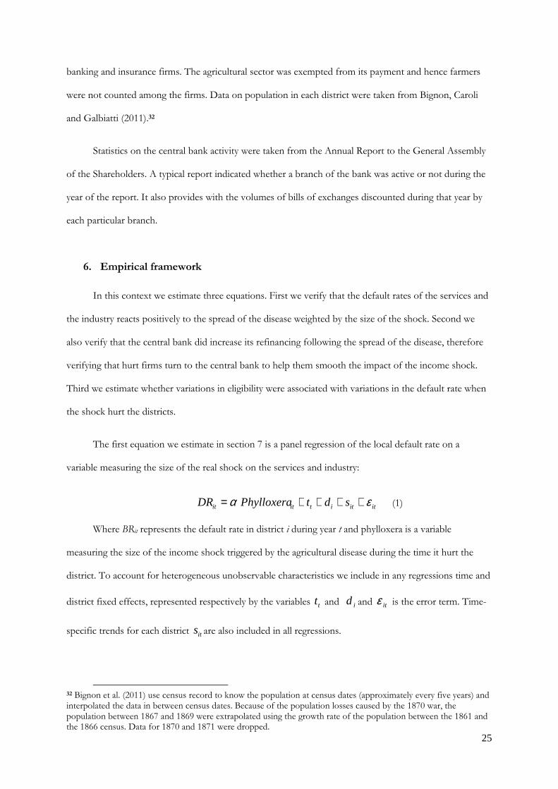
The first equation we estimate in section 7 is a panel regression of the local default rate on a

variable measuring the size of the real shock on the services and industry:

ititititit sdtPhylloxeraDR εα ++++= (1)

Where BRit represents the default rate in district i during year t and phylloxera is a variable

measuring the size of the income shock triggered by the agricultural disease during the time it hurt the

district. To account for heterogeneous unobservable characteristics we include in any regressions time and

district fixed effects, represented respectively by the variables tt and id and itε is the error term. Time-

specific trends for each district its are also included in all regressions.

32 Bignon et al. (2011) use census record to know the population at census dates (approximately every five years) and interpolated the data in between census dates. Because of the population losses caused by the 1870 war, the population between 1867 and 1869 were extrapolated using the growth rate of the population between the 1861 and the 1866 census. Data for 1870 and 1871 were dropped.

26

In a second specification we check that the central bank has indeed increased refinancing following

the arrival of the disease in the district i controlling for the number of branches operated by the central

banks in the district.

ititititititit sdtBranchAuxBranchShockDV εγβα ++++++= . (2)

Where itDV stands for discounting volumes of the central bank in district i during year t and

itBranch is the number of branches and itBranchAux. is the number of auxiliary branches in district i

during year t. In order to account for structural determinants and the secular evolution in the discount

volumes the regressions include districts and year fixed effects and trends specific to each district.

The third equation estimates whether the default rate of the districts with greater eligibility

increased less than in districts with lower eligibility when the districts were hurt by the agricultural

productivity shock. We estimate regressions of the default rate on the shock, a measure of the eligibility

and the interacted variable of the shock multiplied by eligibility. Formally:

ititititititit sdtEligShockEligShockDR εγβα ++++++= * (3)

Where itDR is the default rate of services and industry firms in district i during year t, itShock

measures the impact of the disease in district i during year t and itElig is a measure of agents’ access to

the central bank refinancing facility in district i during year t. The regressions include districts and year

fixed effects and time-specific trend for each district. In a fourth specification we run the same regressions

as in (3) but add variables that control for the location choice of the central bank branches.

7. Results

7.1. Phylloxera Vastatrix, the bug that shocked the French economy

The phylloxera vastatrix (or the devastator of vines) is a near microscopic insect that started to

affect French vineyards in the 1860s (Gale, 2011, p. 18). The yellow aphid sinks its pointed snout into the

roots and sucks out the sap. Its saliva infects the root at the attacked points preventing the wound from

healing. This way the phylloxera not only causes the yield to fall to zero but kills the plants themselves in a

short time. The approximate time between the arrival of the pest and the death of the plant is about a year

27

(Pouget, 1990). The aphid spread gradually over the territory, though its speed of destruction was not

uniform across time and space. For example between 1871 and 1879 the Gard lost 83% of its vineyards

while the neighbouring Herault lost only 59% (Lachiver, 1988, p. 416).

The effects of the aphid were first noticed in 1863 near the Rhone river in the South of France, and

soon thereafter in the Bordeaux region. Yet it took a long time to understand why the vines were dying

and even longer to understand what could be done about it. The insect was first identified as linked to the

symptoms in 1868, after the study of a dead vineyard near the Rhône by the botany professor Jules E.

Planchon. After that identification, the scientific debate raged during seven years before the scientific

community agreed that the bug was the cause –and not just a consequence– of the disease. Academics

tried various treatments to fight the pest but none of those trials proved helpful for winegrowers (Pouget,

1990). It is only in 1890 that the cure to the epidemic was found and popularized. The solution involved

grafting European vines onto phylloxera-resistant American stock.

The arrival of phylloxera caused a brutal reduction of wine-growers revenues. In a mostly

agricultural country, wine production represented 6.4% of the pre-aphid 1862 GDP. In 1890 the revenues

from wine production had dropped to 2.75% of French GDP.33 In 1870 wine represents a source of

income for 21% of the population (Millardet, 1877, p. 82). Price increases did not compensate for the fall

in quantity (Banerjee et al. 2010) and the impact of the aphid onto the local economy were sometimes

disastrous (Postel-Vinay, 1989). However, its impact varied a lot across districts, as some of them did not

grow any vines while in others wine production could reach up to 54% of the local GDP. Wine

production represented 9.2% of wine producing districts GDP. Figure 3 shows the distribution of the

shares of wine production in percentage of the district GDP in 1862.

The shock induced by phylloxera did not impact consumers’ budget markedly. Indeed the increase

of the farm-gate price of wine was not accompanied by an increase in the consumption price.34 The price

of wine in Paris was pretty stable during the whole period. Three main reasons explain this stability of

consumer price. First wine imports increased sharply. Second the practice of vine cultivation spread

quickly in the (phylloxera-free) French colonies in North-Africa, notably Algeria. Third various wine

33 See Bignon, Caroli and Galbiati (2011). 34 Simpson (2011, p. 34-5).

28

adulteration techniques were allowed to maintain the total quantity of alcoholic beverages created from

the pressing of grapes. The second wines (called piquette) made by adding sugar to the cakes that remained

after the first pressing were sold on the market in the 1880s.

The impact of this huge shock on the agricultural sector was smoothed neither by fiscal nor

monetary policy. The central bank was prohibited from lending against any assets that had been originated

in the agricultural sector.35 Fiscal policy was of little help: the state spent 1 million Francs a year on

phylloxera at the apex of the disease in the 1880s and this money was directed toward scientific research

(Loubère, 1978, p. 172). Moreover no welfare program such as unemployment benefits existed to smooth

the revenues losses (Bignon et al., 2011).

Figure 3: The share of wine production in the district GDP in 1862

Sources: Authors computations using Galet (1957) and Delafortrie and Morice (1959).

The length of the episode (from 1863 to 1890) made it impossible for farmers to maintain their

consumption by drawing down savings. It is also very unlikely that farmers were able to increase their

saving in advance of the income shock. This would have required a clear understanding of how the disease

spread and of its cause, an issue that was not settled before 1875 (Gale, 2011, chapter 1). Yet the final

agreement that the aphid caused the disease did not make the French wiser in using the spread of the

insect over the territory as a signal of future losses. The literature identifies two reasons for this. Some

35 It is only in 1898 that the law was amended to allow the Banque de France to lend against bills of exchanges issued by farmers or any agricultural firms.

29

argued that the disease would be confined by nature to some regions, while other simply denied its

existence, arguing that the disease could be avoid by taking good care of the vines (Gale, 2011, p. 52).

Loubère (1978, p. 158) argued that such a blindness resulted from the policy of uprooting the diseased

vines as a mean to safeguard those still intact.

Figure 4: Revenues from wine production and the spread of the phylloxera, 1862 – 1890

Source: Authors from INSEE (1946, p. *90) and Galet (1957).

We conclude from this examination that the shock created by phylloxera on the French economy

must have been transmitted to the other sectors of the economy. This transmission should have decreased

the other sectors revenues.36 One way to measure the importance of the shock on agriculture is by

comparing the revenues from wine production withthe proportion of districts in which the aphid was

spotted in at least one vineyard (Figure 4). A more formal test of the relationship between the spread of

the phylloxera and the economy is given by the study of the impact of the phylloxera on the default rate in

the districts hit by the phylloxera. As outlined above, one of the advantages of using the default rate is that

36 This negative liquidity shock could have impacted the local economy either directly or indirectly. Indeed the fall of wine-growers’ revenues could have triggered a fall in their demand to the other sectors. But it could also have been that the collapse of some banks in the most attained regions – a phenomenon described by Postel-Vinay (1989) – could have restricted the quantity of credit available to the other sectors of the economy. The data does not exist to test for the importance of each of those channels.

30

it does not include farmers or any other agricultural firms. Hence the dependant variable is a pure measure

of the indirect impact of the shock on the local economy restricted to the services and industrial sectors.

Table 1 displays the results of the regression analysis. All the residuals are clustered at the district

level. The results show that the shock created by the phylloxera increased significantly the default rate of

firms of the services and industry, with the only exception being for the variable “Presenceij”. One

explanation for this non-significance is the fact this variable considers that the phylloxera shocked the

district economy right from its arrival in the first vineyard, which, given the history of the spread of the

aphid is clearly a very strong assumption. Historians noted that it takes some time for the aphid to destroy

a significant proportion of the vineyards of a district.37 Overall our results are consistent with our claim

that, once the aphid spread in a district, the absence of a proper and sufficiently cheap treatment to

prevent the vines from dying constituted a negative shock to the productive assets of farmers that was

transmitted to the other sectors.

Table 1: Regression analysis of the impact of the phylloxera on the default rate of the services and industrial sectors of the same district.

------------------------------------------------------------

(1) (2) (3)

Independent variable: Default rate in % at district level

------------------------------------------------------------ Presenceij 0.0533

0.0702

Shockij 0.1023*

0.0603

W_shockij 0.2815** 0.1401

Trend 0.00340*** 0.00338*** 0.00338***

0.00002 0.00002 0.00002

------------------------------------------------------------

N 7363 7363 7363 r2 0.474 0.475 0.476

------------------------------------------------------------ All specifications include year and district fixed effects and district specific time trends. Residuals are clustered at the district level. * p<0.1, ** p<0.05, *** p<0.01

7.2. Phylloxera, the Banque de France and the default rate

The arrival of phylloxera had a clear impact on the local economy. Did it also affect the activity of

the Banque de France? Section 4 argued that the decision of the Banque de France to create new branch

37 This interpretation is even more likely if one notes that the only differences between ga_wg and p_wg is the starting year of the epidemics in a district.

31

offices was driven by long-term, structural considerations and not by short-term developments, let alone

in response to a negative shock at the local level. However, this does not mean that the Banque de France

would not feel the repercussions of economic stress in the districts hit by phylloxera. By design the

Banque de France stood ready to lend to (or more precisely to buy bills from) all solvent eligible

counterparties if they required so.

Table 2 gives the result of a regression of the annual volume of BdF discounting on the district

level. As in table 2 we use three different measures for the shock induced by phylloxera: a dummy variable

that becomes one as soon as phylloxera arrives (Presenceij), a dummy variable that becomes one as soon as

phylloxera arrives and the production falls below its pre-phylloxera level (Shockij) and a third variable that

weight Shockij by the actual decline in production relative to the pre-phylloxera level (W_shockij). The three

shock measures are weighted by the share of the wine production in the district GDP. Two variables

control for the size of BdF operations in the district, namely the number of full branch offices and the

number of smaller auxiliary offices. District and time fixed effects to account for structural differences

between districts and temporary shocks at the national level. Also included are district specific time trends

that capture differences in the secular development of the districts.

Table 2: The impact of phylloxera on Banque de France discounting

------------------------------------------------------------

(1) (2) (3)

Independent variable: Annual volume discounted by the BdF per

département in million francs ------------------------------------------------------------

Presenceij 58.00*

(34.18)

Shockij 56.72

(36.05) W_shockij 34.87**

(16.58)

# BdF 44.98* 44.11* 42.92*

branches (22.90) (22.55) (22.48)

# BdF auxiliary 35.56 35.21 34.99

offices (28.33) (28.25) (28.24) Trend 0.63*** 0.61*** 0.47***

(0.12) (0.11) (0.02)

------------------------------------------------------------

N 4502 4502 4502

r2 0.820 0.820 0.820 ------------------------------------------------------------

The variables measuring the shock Presenceij, Shockij and W_shockij are weighted by the share of wine production in the district GDP. All specifications include year and district fixed effects and district specific time trends. Residuals are clustered at the district level. Standard errors in parentheses. Significance levels: * p<0.1, ** p<0.05, *** p<0.01.

32

As can be seen in table 2, all variables have the expected sign. The volume of discounting increases

over time (trend positive and significant) and increases when new branch offices are opened (the

coefficient on auxiliary offices is also positive but not significant). The arrival of phylloxera increases the

demand for discounting at the BdF in all three specifications; in the specification that arguably captures

the shock to the best extent (plij) the coefficient is statistically significant at the 5% level. In the other

specifications the coefficients are not significant or are only marginally so at the 10% level. This is not too

surprising. The effect of phylloxera on discounting goes both ways. While phylloxera acted as a income

shock for the non-agricultural sectors, increasing the demand for some sort of bridge financing, it also

depressed in the medium term economic activity and income at the district level, thereby decreasing the

demand for money and finally demand at the BdF discount window. The result shows that the income

shock was strong enough to make the coefficient of the shock variable greater than zero –constituting

strong evidence that the central bank provided liquidity support in the districts affected by phylloxera.

This allows turning to the main empirical question of the paper – did access to BdF rediscounting

facilities soften the impact of phylloxera on the district default rate? Table 3 gives the results from several

specifications using the three different measures for phylloxera described above and three different

variables accounting for the impact of the Banque de France. Because eligibility as counterparty was tied

to the presence or not of a BdF branch, the first set of estimates uses simply the number of branches

within the district. The other two measures adjust for the size of the district (larger districts needing more

branches to have the same degree of access to the BdF) and for the population of the district (more

densely populated districts having more cities needing more branches to have the same degree of access to

the BdF). Neither of the measures is clearly superior to the others and so all three are reported. As before

district and time fixed effects as well as district specific time trends are included to control for the many

other determinants of the default rate that cannot be captured by the explaining variables included.

The key variable of interest is the interaction between the shock and access to the BdF. If the BdF

had a positive impact in the districts affected by phylloxera the interaction term should be negative,

implying a lower default rate than if fewer access to the BdF had been available. As can be seen in table 4

33

the interaction term always has the negative sign as predicted, and in most specifications the coefficient is

also strongly statistically significant. Access to the Banque de France prevented to some extent the

agricultural crisis from spilling over to solvent but liquidity-constrained firms in the rest of the local

economy. Also interesting are the coefficients on the shock variable. In comparison to the specifications

excluding a variable for BdF branching as reported in table 2, taking account of the presence or not of the

BdF increases the significance level of the shock variable, in particular if the plij variable is used for

measuring the shock. This implies that distinguishing between districts with access to the BdF and districts

without such access helps to better identify the impact of phylloxera on the local default rate. Finally, the

coefficient on the BdF branches is negative and sometimes significant, but there a priori no reason to

expect a positive or negative relation between BdF branching and the evolution of the default rate.

Table 4 repeats the exercise including in addition to the trend and fixed effects some control

variables that might provide extra explanatory power for the default rate. The number of firms per 1000

inhabitants and population density both capture economic development and differences in the economic

structure between districts. The coefficients on both variables are always significant; the negative signs

implying that districts with more economic and entrepreneurial activity were also those with ceteris

paribus lower default rate. The variable farmsize*shock was included in order to account for regional

variation in the structure of winegrowing that might lead to a different impact of phylloxera on regional

income and liquidity, e.g. because smaller farms have less outside resources available or – quite contrary –

because smaller farms are more diversified. In any case, the coefficient is never statistically significant.

Finally we include the number of commercial bank branches in the district. As laid out in section 4,

commercial banks, most notably the Crédit Lyonnais and the Société Générale, created extensive branch

networks starting in the 1860s. It could be argued that these branch networks could substitute for a

missing Banque de France branch by equally providing lending to a local economy hit by a liquidity shock.

The coefficient on the interaction term between commercial bank branching and phylloxera is surprisingly

positive (implying a higher default rate when a commercial bank was present), even if almost never

statistically significant. Apparently commercial bank branches were no suitable substitute for a branch.

The inclusion of these additional explanatory variables does not alter the results from the simple

baseline estimations in table 3. In particular the shock variable and the interaction between shock and BdF

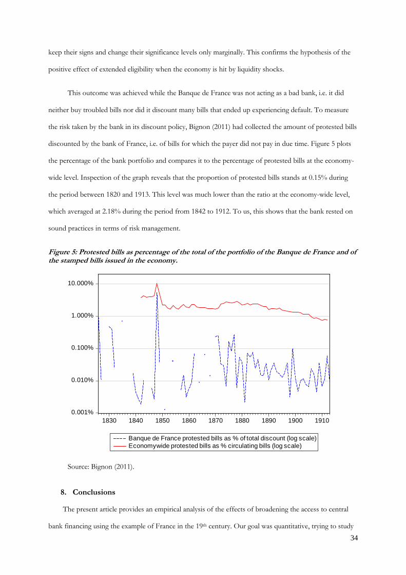
34

keep their signs and change their significance levels only marginally. This confirms the hypothesis of the

positive effect of extended eligibility when the economy is hit by liquidity shocks.

This outcome was achieved while the Banque de France was not acting as a bad bank, i.e. it did

neither buy troubled bills nor did it discount many bills that ended up experiencing default. To measure

the risk taken by the bank in its discount policy, Bignon (2011) had collected the amount of protested bills

discounted by the bank of France, i.e. of bills for which the payer did not pay in due time. Figure 5 plots

the percentage of the bank portfolio and compares it to the percentage of protested bills at the economy-

wide level. Inspection of the graph reveals that the proportion of protested bills stands at 0.15% during

the period between 1820 and 1913. This level was much lower than the ratio at the economy-wide level,

which averaged at 2.18% during the period from 1842 to 1912. To us, this shows that the bank rested on

sound practices in terms of risk management.

Figure 5: Protested bills as percentage of the total of the portfolio of the Banque de France and of the stamped bills issued in the economy.

Source: Bignon (2011).

8. Conclusions

The present article provides an empirical analysis of the effects of broadening the access to central

bank financing using the example of France in the 19th century. Our goal was quantitative, trying to study

10.000%

1.000%

0.100%

0.010%

0.001%1830 1840 1850 1860 1870 1880 1890 1900 1910

Banque de France protested bills as % of total discount (log scale)Economywide protested bills as % circulating bills (log scale)

35

whether a widening of the eligibility criteria helped stabilizing economies hit by temporary negative

liquidity shocks. The empirical results show that this may have been the case. The empirical analysis is

based on a newly assembled dataset tracing the economic evolution of all French districts during the

period from 1826 to 1913. The local default data is complemented by qualitative and quantitative material

on the details on the monetary policy framework documenting the determinants of the eligibility and

collateral policy of the French central bank. In the 19th century only enterprises and people living in a city

or town where the Banque de France was represented could obtain central bank loans. This feature of the

framework of the Banque de France allows circumventing the empirical challenges of assessing the impact

of eligibility by exploiting the geographical dimension of central bank access in France, as we can argue

that the opening of branches by the central bank was never endogenous to the various shocks that hit the

local economy, but rather the outcome of a negotiation between the government and a private maximizing

monopoly in search for the renewal of its privilege of banknote issuance.

To assess the importance of central bank eligibility for economic agents hit by a liquidity shock, we

relied on the consequences of a shock to agricultural productivity on the default rate in the industrial and

the service sectors, phylloxera. The arrival and spread of phylloxera increased the default rate of the firms

of those sectors and the volume of bills discounted by the Banque de France in the affected districts.

However, as the empirical results show, the impact of the shock was smaller when the agents in the

affected region had access to liquidity through the central bank. Decreasing the transaction cost of

accessing liquidity in times of a higher need for liquidity then had a positive impact on local firms. At the

same time, the Banque the France did not act as a “bad bank”, taking over worthless assets. Lending by

the central bank followed strict rules and the Banque de France never discounted bills of bad quality. The

spread of the phylloxera coincided indeed with a secular decline in the proportion of defaulted bills in the

portfolio of the Banque de France.

The fact that the extension of eligibility via the creation of new branch offices was not driven by

stress in the financial sector but is due to structural reasons of course also implies that the positive results

of the extension of eligibility were not the result of an explicit policy by the bank. The argument however

adds a new channel through which central bank branching might have affected the real economy. Jobst

(2010) has documented the European-wide phenomenon of central bank branching during the 19th

36

century. For some countries there is evidence that central bank branching led to a convergence of regional

interest rates.38 As eligibility was in many countries tied to residency, i.e. a geographic criterion, the

smoothing effect in the case of liquidity shocks might be well observable in other European countries as

well. More generally, eligibility of counterparties and also assets deserves more attention in historical

research, in particular given the importance eligibility has acquired in recent years. If there is any lesson to

draw from this past experience in terms of today’s monetary policy, our results support the emphasis put

carefully choosing the counterparties and assets that should be eligible at the central banks.

References

Acharya,Viral, Gromb Denis and Tanju Yorulmazer, 2012, Imperfect Competition in the Interbank

Market for Liquidity as a Rationale for Central Banking?” American Economic Journal: Macroeconomics,

4(2), 184-217.

INSEE, 1946, Annuaire statistique INSEE, Paris : Imprimerie Nationale

Banerjee, Abhijit, Esther Duflo, Gilles Postel-Vinay and Timothy M. Watts, 2010, Long Run Health

Impacts of Income Shocks: Wine and Phylloxera in 19th Century France, Review of Economics and

Statistics, 92(4), 714-728.

Bignon Vincent, Caroli, Eve and Galbiati Roberto, 2011, Stealing to Survive: Crime and Income Shocks in

19th Century France, Working Paper CEPREMAP - PSE 1111.

Bignon Vincent, 2011, Funding Crises and the Bankruptcy Rate in the very long-run: France during the

19th century, mimeo.

Bindseil, Ulrich, 2009, Central bank financial crisis management from a risk management perspective, In:

Bindseil et al. (eds.). Risk Management for Central Banks and Other Public Investors. Cambridge:

Cambridge University Press. 394–439.

Bodenhorn, Howard, 2000, A History of Banking in Antebellum America: Financial Markets and Economic

Development in an Era of Nation-Building, Cambridge: Cambridge University Press.

38 See Good (1977) on Austria and Ohnuki (2007) and Mitchener and Ohnuki (2009) on early 20th century Japan. Bodenhorn (2000), however, is sceptical on the integration effect of the Second Bank of the United States.

37

Bordo, Michael, 1990, The lender of last resort: Alternative views and historical experience, Federal Reserve

Bank of Richmond Economic Review, January/February, pp. 18-29.

Borio, Claudio, 2001, A hundred ways to skin a cat: Comparing monetary policy operating procedures in

the United States, Japan and the Euro Area. BIS Paper 9. 1–22.

Borio, Claudio and Piti Disyatat, 2009, Unconventional monetary policy: an appraisal, BIS Working Paper

292.

Calomiris, Charles, 1994, Is the discount window necessary? A Penn-Central perspective, Federal Reserve

Bank of St. Louis Review, 76 (3), pp. 31-56.

Cameron, Rondo, 1961, France and the Economic Development of Europe 1800-1914, Princeton :

Princeton University Press.

Cameron, Rondo, 1967, Banking in the Early Stage of Industrialization, Oxford University Press

Carlson, Mark, Mitchener, Kris J. and Gary Richardson, 2011, Arresting Banking Panics: Federal Reserve

Liquidity Provision and the Forgotten Panic of 1929, Journal of Political Economy, Vol. 119(5), pp.

889-924.

Chailloux, Alexandre, Simon Gray and Rebecca McCaughrin, 2008: Central bank collateral frameworks:

Principles and policies. IMF Working Paper 222.

Cechetti, Stephen G., 2009, Crisis and Responses: The Federal Reserve in the Early Stages of the Financial

Crisis, Journal of Economic Perspectives, Vol. 23(1), pp. 51-76.

Cuardia, Vaco and Michael Woodford, 2011, The Central Bank Balance-Sheet as an Instrument of

Monetary Policy, Journal of Monetary Economics 58, p. 54-79

Dalloz Victor Alexis, 1830, Traité des effets de commerce, Paris : Tarlier.

Delafortrie, Nicole and Janine Morice, 1959, Les revenus départementaux en 1864 et 1954, Paris : Librairie

Armand Colin.

ECB, 2009, The implementation of monetary policy since August 2007, Monthly Bulletin, July.

ECB, 2011, The ECB's non-standard measures - impact and phasing-out, Monthly Bulletin, July.

38

Eggertsson, Gauti B. and Michael Woodford, 2003. The Zero Bound on Interest Rates and Optimal

Monetary Policy, Brookings Papers on Economic Activity vol. 34(1), pages 139-235.

Farmer, Roger, 2012, Qualitative Easing: How it Works and Why it Matters”, NBER Working Paper No.

18421, September.

Flannery, Marc, 1996, Financial crises, payment system problems, and discount window lending, Journal of

Money Credit and Banking 28, pp. 804-824.

Freixas, Xavier, Giannini Curzio, Glenn Hoggarth and Farouk Soussa, 2000, Lender of last resort: What

have we learned since Bagehot? Journal of Financial Services Research 18(1), p. 63-84.

Gale, George, 2011, Dying on the Vine: How Phylloxera Transformed Wine, University of California

Press

Galet, Pierre, 1957. Cépages et vignobles de France, Montpellier : Imp. du Paysan du Midi.

Gertler, Mark and Peter Karadi, 2012, A Framework for Analyzing Large Scale Asset Purchases as a

Monetary Policy Tool, May 2012.

Gille, Bertrand, 1959, La banque et le crédit en France de 1815 à 1848, Paris: Presses universitaires de France.

Gille, Bertrand, 1970, La Banque en France au XIXe siècle, recherches historiques, Geneva, Paris: Droz.

Good, David, 1977, Financial integration in late 19th century Austria, Journal of Economic History, 37.

Goodfriend, Marvin and Robert G. King, 1988, Financial deregulation, monetary policy and central

banking. Federal Reserve Bank of Richmond Economic Review 74 (3) pp. 3-22.

Heider, Florian and Marie Hoerova, 2009, Interbank Lending, Credit-Risk Premia, and Collateral,"

International Journal of Central Banking vol. 5(4), pages 5-43.

Heider, Florian, Maria Hoerova and Cornelia Holthausen, 2009, Liquidity hoarding and interbank market

spreads: the role of counterparty risk, ECB working paper 1169.

Holmström, Bengt and Jean Tirole, 1998, Private and Public Supply of Liquidity, Journal of Political

Economy 106(1), p. 1-40

39

Jobst, Clemens, 2010, Gouverner une banque centrale décentralisée: l’exemple austro-hongrois (1847-

1914), in O. Feiertag, & M. Margairaz (eds.), Gouverner une banque centrale: du XVIIe siècle à nos jours.

Paris: Albin Michel, 113-42.

Kareken, John H. and Neil Wallace, 1978, Deposit Insurance and Bank Regulation: A Partial Equilibrium

Exposition, Journal of Business 51(3), p. 413-438)

Lachiver, Marcel, 1988, Vins, vignes et vignerons: Histoire du vignoble français, Paris : Fayard.

Lescure Michel, 2003 , La formation d’un système de crédit en France et le rôle de la banque d’émission

(1850-1914), in Politiques et pratiques des banques d’émission en Europe (XVIIe – XXe siècle). Eds by O.

Feirtag and M. Margairaz. Paris: Albin Michel. 131-148.

Loubère, Leo A., 1978, The Red and the White: A History of Wine in France and Italy in the 19th century,

State University Of New York Press.

Meltzer, Allan, 2003, A history of the Federal Reserve, Volume I 1913-1951. Chicago: University of Chicago

Press.

Millardet, Alexis, 1877, La question des vignes américaines du point de vue théoqique et pratique,

Bordeaux : Féret et fils

Mitchener, Kris and Mari Ohnuki, 2009, Institutions, Competition, and Capital Market Integration in

Japan.Journal of Economic History vol. 69(1), pp. 204-37.

Nishimura, Shiyuza, ‘The French provincial banks, the Banque de France, and bill finance, 1890–1913’,

Economic History Review, XLVIII (1995), pp. 536–54.

Ohnuki, Mari,2007, The Bank of Japan Network and Financial Market Integration: From the

Establishment of the Bank of Japan to the Early 20th Century, Monetary and Financial Studies, vol

25(1), p. 95-128.

Percerou, Jean, 1935, Faillites, banqueroute et liquidations judiciaires, Paris : Rousseau.

Plessis, Alain, 1985, Regents Et Gouverneurs de la Banque de France, Genève : Librairie Droz

Plessis, Alain (1999), Les banques locales, de l’essor du Second Empire à la « crise » de la Belle Époque, in

M. Lescure et A. Plessis (Eds.), Banques locales et régionales en France au 19ème siècle. Paris:

Albin Michel, 202-233.

40

Postel-Vinay Gilles, 1989, Debts and Agricultural Performance in the Languedocian Vineyard, 1870–1914,

in Agrarian Organization in the Century of Industrialization: Europe, Russia, and North America, G.

Grantham and C. S. Leonard (Eds.), Greenwich, CT: JAI Press. 161–186

Pouget, R., 1990, Histoire de la lutte contre le phylloxéra de la vigne en France, Paris : INRA.

Prunaux, Emmanuel, 2009, Les comptoirs d’escompte de la banque de France 2e partie, Napoleonica n°3, p.

49-98.

Quinn, Stephen and William Roberds 2012. "Responding to a shadow banking crisis: the lessons of 1763,"

Working Paper 2012-08, Federal Reserve Bank of Atlanta.

Ramon, Gabriel G., 1929, Histoire de la Banque de France d'après les sources originales. Paris : B. Grasset, 503 p.

Roulleau, Gaston, 1914, Des règlements par effets de commerce en France et à l’étranger, Paris : Imprimerie

Dubreuil, Frèrebeau et Cie. 204 p.

Repullo, Rafael, 2000, Who should act as a lender of last resort? An incomplete contracts model, Journal of

Money,Credit,and Banking, 32, pp. 580–605

Richardson, Gary and William Troost, 2009, Monetary Intervention Mitigated Banking Panics During the

Great Depression: Quasi-Experimental Evidence from a Federal Reserve District Border, 1929 to

1933, Journal of Political Economy, vol. 117(6), pp. 1031-1073.

Schwartz, Anna, 1992, The misuse of the Fed’s discount window, Federal Reserve Bank of St. Louis Review

1992 (October) pp. 58-69.

Simpson, James, 2011, Creating Wine: The Emergence of a World Industry, 1840-1914, Princeton

University Press.

Toutain, Jean-Claude, 1987, Le produit intérieur brut de la France de 1789 à 1982, Economies et sociétés :

Histoire quantitative de l'économie française 15.

Ugolini, Stefano, 2012, The Origins of Foreign Exchange Policy: the National Bank of Belgium and the

Quest for Monetary Independence in the 1850s, European Review of Economic History 16(1), p. 51-73.

41

Table 3. Regression results simple specification

------------------------------------------------------------------------------------------------------------------------------------------------------------

Dependent variable: District default rate in %

BdF variable: Number of BdF branches Branches/km2 Branches/1000 inhabitants

Shock variable: Presenceij shockij W_shockij Presenceij shockij W_shockij Presenceij shockij W_shockij

(1) (2) (3) (4) (5) (6) (7) (8) (9)

------------------------------------------------------------------------------------------------------------------------------------------------------------

Shock 0.082 0.178 0.660*** 0.060 0.135 0.533** 0.151** 0.241*** 0.722***

0.094 0.115 0.229 0.082 0.103 0.224 0.071 0.083 0.257

BdF -0.016* -0.016 -0.015 -0.103*** -0.103*** -0.103*** -1.729 -1.574 -1.798

0.009 0.009 0.009 0.022 0.023 0.023 3.585 3.602 3.506

BdF*shock -0.103* -0.152** -0.445*** -0.500 -0.708* -2.125*** -62.882*** -82.289*** -203.427***

0.061 0.064 0.111 0.401 0.425 0.806 18.784 20.197 60.980

Trend 0.0029*** 0.0029*** 0.0029*** 0.0030*** 0.0030*** 0.0030*** 0.0028*** 0.0028*** 0.0028***

0.0002 0.0002 0.0002 0.0002 0.0002 0.0002 0.0002 0.0002 0.0002

------------------------------------------------------------------------------------------------------------------------------------------------------------

N 7363 7363 7363 7363 7363 7363 7191 7191 7191

r2 0.545 0.545 0.546 0.547 0.547 0.548 0.542 0.543 0.543

------------------------------------------------------------------------------------------------------------------------------------------------------------

All specifications include year and district fixed effects and district specific time trends. Residuals are clustered at the district level.

“Presence” accounts only for the presence of the aphid in the district. “shockij” excludes the years when the aphid is present but did not had triggered sufficient

losses to wine production. “W_shockij” weighted shockij by the size of the loss of wine production. The three variables are weighted by the size of wine production

in the 1862 GDP.

* p<0.1, ** p<0.05, *** p<0.01

42

Table 4. Regression results including additional controls

------------------------------------------------------------------------------------------------------------------------------------------------------------

Dependent variable: District default rate in %

BdF variable: Number of BdF branches Branches/km2 Branches/1000 inhabitants

variable: Presenceij shockij W_shockij Presenceij shockij W_shockij Presenceij shockij W_shockij

(1) (2) (3) (4) (5) (6) (7) (8) (9)

------------------------------------------------------------------------------------------------------------------------------------------------------------

Shock 0.354* 0.423* 1.225*** 0.253 0.294* 0.972** 0.227 0.254* 1.021**

0.208 0.222 0.388 0.162 0.170 0.388 0.147 0.148 0.410

BdF -0.017* -0.016* -0.016* -0.127*** -0.125*** -0.128*** -2.102 -1.912 -2.326

0.009 0.009 0.009 0.029 0.029 0.029 3.570 3.571 3.467

BdF*shock -0.284* -0.372** -0.764** -1.324* -1.813** -2.895 -80.911** -110.102*** -220.966*

0.143 0.160 0.364 0.694 0.784 1.864 34.920 38.842 120.087

Firms per 1000 . -2.837** -2.974** -2.838** -2.673* -2.798** -2.618* -2.820** -2.913** -2.731*

inhabitants 1.420 1.391 1.359 1.403 1.367 1.377 1.411 1.363 1.387

Population -0.00010*** -0.00010*** -0.00010*** 0.00007 0.00007 0.00007 -0.00011*** -0.00011*** -0.00011***

density 0.00003 0.00003 0.00003 0.00005 0.00005 0.00005 0.00003 0.00003 0.00003

Branches of CL/SG -0.014 -0.014 -0.011 -0.017 -0.017 -0.015 -0.012 -0.012 -0.010

per km2 0.014 0.014 0.013 0.013 0.013 0.013 0.013 0.013 0.012

CL/SG*shock 0.283 0.358 0.824* 0.239 0.299 0.602 0.167 0.161 0.512

0.185 0.226 0.477 0.162 0.203 0.461 0.117 0.148 0.413

Farmsize*shock -0.019 -0.015 -0.086 -0.013 -0.007 -0.088 -0.008 0.005 -0.075

0.019 0.024 0.061 0.020 0.025 0.068 0.022 0.028 0.072

Trend 0.0041*** 0.0042*** 0.0041*** 0.0042*** 0.0043*** 0.0041*** 0.0039*** 0.0040*** 0.0039***

0.0005 0.0005 0.0005 0.0005 0.0005 0.0005 0.0005 0.0005 0.0005

------------------------------------------------------------------------------------------------------------------------------------------------------------

N 6968 6968 6968 6968 6968 6968 6968 6968 6968

r2 0.545 0.545 0.547 0.548 0.548 0.549 0.544 0.544 0.545

------------------------------------------------------------------------------------------------------------------------------------------------------------

All specifications include year and district fixed effects and district specific time trends. Residuals are clustered at the district level.

* p<0.1, ** p<0.05, *** p<0.01