Can a Lender of Last Resort Stabilize Financial Markets

NBER WORKING PAPER SERIES

CAN A LENDER OF LAST RESORT STABILIZE FINANCIAL MARKETS? LESSONSFROM THE FOUNDING OF THE FED

Asaf BernsteinEric Hughson

Marc D. Weidenmier

Working Paper 14422http://www.nber.org/papers/w14422

NATIONAL BUREAU OF ECONOMIC RESEARCH1050 Massachusetts Avenue

Cambridge, MA 02138October 2008

The authors would like to thank Richard Burdekin, Vincenzo Quadrini and seminar participants at Claremont McKenna College and the University of Southern California for comments. The viewsexpressed herein are those of the author(s) and do not necessarily reflect the views of the NationalBureau of Economic Research.

NBER working papers are circulated for discussion and comment purposes. They have not been peer-reviewed or been subject to the review by the NBER Board of Directors that accompanies officialNBER publications.

© 2008 by Asaf Bernstein, Eric Hughson, and Marc D. Weidenmier. All rights reserved. Short sectionsof text, not to exceed two paragraphs, may be quoted without explicit permission provided that fullcredit, including © notice, is given to the source.

Can a Lender of Last Resort Stabilize Financial Markets? Lessons from the Founding of theFedAsaf Bernstein, Eric Hughson, and Marc D. WeidenmierNBER Working Paper No. 14422October 2008JEL No. E4,G1,N11,N12

ABSTRACT

We use the founding of the Federal Reserve as a historical experiment to provide some insight intowhether a lender of last resort can stabilize financial markets. Following the Panic of 1907, Congresspassed two measures that established a lender of last resort in the United States: (1) the Aldrich-VreelandAct of 1908 which authorized certain banks to issue emergency currency during a financial crisis and(2) the Federal Reserve Act of 1913 which established a central bank. We employ a new identificationstrategy to isolate the effects of the introduction of a lender of last resort from other macroeconomicshocks. We compare the standard deviation of stock returns and short-term interest rates over timeacross the months of September and October, the two months of the year when financial markets weremost vulnerable to a crash because of financial stringency from the harvest season, with the rest ofthe year during the period 1870-1925. Stock volatility in the post-1907 period (June 1908-1925) wasmore than 40 percent lower in the months of September and October compared to the period (1870-May 1908). We also find that the volatility of the call loan rate declined nearly 70 percent in Septemberand October following the monetary regime change.

Asaf BernsteinHarvey Mudd College500 East Ninth StreetClaremont, CA [email protected]

Eric HughsonLeeds School of BusinessUniversity of ColoradoBuilding #4, UCB 419Boulder, CO [email protected]

Marc D. WeidenmierDepartment of EconomicsClaremont McKenna CollegeClaremont, CA 91711and [email protected]

1

The recent sub-prime mortgage crisis in the United States raises serious questions

about the role of monetary policy in a financial crisis. The Federal Reserve responded to

the credit crunch by lowering the Federal Funds Rate from 5.25 percent in September

2007 to 1.5 percent in early October 2008. The central bank has followed up interest rate

cuts by orchestrating bail-outs of AIG, Fannie Mae, Freddie Mac, and Wall Street Firm

Bear Stearns which was heavily invested in sub-prime mortgages. Several leading

economists including Paul Volcker, former Chairman of the Federal Reserve, have

questioned whether the Fed can legally take over control of insolvent financial

institutions (International Herald Tribune, April 9, 2008). Chairman Bernanke, on the

other hand, argues that the recent actions by the Fed are imperative because “The credit

system is like plumbing: It permeates throughout the entire system. And our modern

economy cannot grow, it cannot create jobs, it cannot provide housing without effectively

working credit markets” (USA Today, September 24, 2008).

Although economists may disagree over whether a central bank should only lend

to solvent firms (as opposed to insolvent and illiquid financial institutions) during a crisis,

one problem acknowledged by both proponents and opponents of activist monetary

policy is that it is very difficult to identify the effect of lender of last resort policies on

financial markets.1 Fortunately, history provides an experiment to test the impact of the

introduction of a lender of last resort on financial markets. Following the Panic of 1907

which was followed by one of the shortest, but most severe recessions in American

1 For a discussion of the importance of a lender of last resort in American economic history, see Bordo (1990). Bernanke and Gertler (2000) argue that central banks should intervene in financial markets to the extent that they affect aggregate demand. Bernanke and Gertler (1989) argue that the balance-sheet effects of asset price decline can reduce investment and economic activity.

1

2

history,2 Congress passed two measures that established a lender of last resort in the

United States: (1) the Aldrich-Vreeland Act of 1908 which temporarily authorized some

banks to issue emergency currency during a financial crisis and (2) the Federal Reserve

Act of 1913 that established a public central bank. The legislation was designed to

provide a “more elastic currency” that could meet the seasonal demands of economic

activity caused by the agricultural cycle. Several of the most severe financial crises of the

National Banking Period (1863-1914) including the Panics of 1873, 1890, 1893, and

1907 occurred in the months of September and October when cash left New York City

banks for the interior of the country to help farmers finance the harvesting of crops

(Kemmerer, 1910; Sprague, 1909).3

The seasonal nature of financial crises in the National Banking Period motivates

the identification strategy employed in this study to isolate the effects of the lender of last

resort function on interest-rate and stock return volatility.4 We compare the standard

deviation of stock returns across the months of September and October over the period

1870-May 1908 with the standard deviation of stock returns in those same months in the

post-Aldrich Vreeland (June 1908-1913) and Federal Reserve (1913-1925) period. We

employ Goetzmann, Ibbotson, and Peng’s (2005) new comprehensive database of pre-

CRSP era stock prices, hereafter GIP, from 1870-1925. The new stock price index

significantly improves on the widely used Cowles Index by using month-end closing

2 The panic of 1907 was precipitated when August Heinze’s attempted short squeeze at United Copper, financed by borrowing from Knickerbocker Trust, collapsed. This caused a series of bank runs which started at the Knickerbocker Trust. This led to a credit crunch and a sharp decline in stock values (Moen and Tallman, 2000). 3 For a discussion of the links between agricultural shocks and recessions in the pre-World War I period, see Davis et al. (2004). 4 Wohar and Fishe (1990), for example, argue that World War I and the closure of the New York financial markets played an important role in the change in the stochastic behavior of interest rates, in addition to the founding of the Federal Reserve. Given that these events all occurred around the same time, they argue that it is difficult to separate out the effects of these different events on time series properties of interest rates.

2

3

prices rather than the average of monthly highs and lows, thereby avoiding a significant

autocorrelation problem in stock returns (Schwert, 1989; Working, 1960).

An analysis of the GIP Index shows that stock volatility in September and

October declined more than 40 percent following the passage of the Aldrich-Vreeland

Act. Although we find that stock volatility in September and October was significantly

greater than the other ten months of the year prior to the passage of Aldrich-Vreeland,

this was not true following the monetary regime change.5 The results are robust to a wide

variety of specification tests with the exception that the result does not hold if we use the

Cowles Index for the empirical analysis. Our findings highlight the potential erroneous

conclusions that can be drawn from using the Cowles Index to study financial markets.

Future research may usefully revisit some questions in financial economics using the new

GIP Index.6 Our analysis supports Friedman and Schwartz’ (1963) hypothesis that

Aldrich-Vreeland and the creation of the Federal Reserve stabilized financial markets

prior to the Great Depression.7

We also examine short-term interest rate volatility in the months of September

and October before and after the monetary regime change. The volatility of the call loan

rate declined by more than 70 percent in the months of September and October following

the passage of Aldrich-Vreeland. Consistent with the analysis of the equity market, 5 Previous studies by Meltzer (2003), Miron (1986) and Mankiw, Miron, and Weil (1988) find that the introduction of the Federal Reserve also reduced the seasonality and level of interest rates. Caporale and Caporale (2003) find that the introduction of the Federal Reserve led to a large reduction in the term premium a six- month debt instruments pays over a three-month one. 6 Some well-known studies that have employed the Cowles Index or Indices from the pre-CRSP era that have the autocorrelation problem include Shapiro (1988), Shiller (1992), and Siegel (2002). Other studies have relied on stock indices such as the Dow which have a very small number of stocks, but do not have significant autocorrelation problems Schwert (1989a, 1989b). 7 Obviously, the results would not hold if we included the Great Depression as part of the analysis. As shown by Miron (1986) the seasonality of interest rates reappeared during the Great Depression because the Fed did not accommodate seasonal money demand. Many studies, most notably Friedman and Schwartz (1963), argue that the Federal Reserve exacerbated the severity of the Great Depression because of tight monetary policy (i.e., the Fed failed to play the role of a lender of last resort).

3

4

interest rate volatility in September and October was significantly greater than the rest of

the year only in the period before the passage of lender of last resort legislation. The

analysis also shows that the reduction in interest rate volatility can be attributed to a

decrease in the standard deviation of the call loan rate, not to a decline in the level and

seasonality of interest rates.8 Overall, the results show that the introduction of a lender of

last resort in the United States dramatically reduced financial market volatility.

We begin the analysis with a brief history of the National Banking Period (1863-

1913) in the pre-World War I period. We then discuss the new database on stock prices in

the pre-CRSP era. This is followed by an empirical analysis of stock and interest rate

volatility. We conclude with a discussion of the implications of our results for future

studies in financial economics and the role of monetary policy during a financial crisis.

II. The National Banking System (1863-1913)

The National Banking Acts of 1863, 1864, an 1865 were passed to raise revenue

to fight the Civil War, create a uniform currency and to standardize the banking system in

the United States. Prior to the passage of the monetary legislation, hundreds of different

currencies circulated at different exchange rates in the United States during the

antebellum period. The Acts required banks to maintain minimum levels of capital,

dependent on the local population where the bank was situated, and deposit a minimum

quantity of eligible bonds with the U.S. Treasury before commencing business.9 National

8 Earlier studies by Miron (1986) and Mankiw, Miron, and Weil (1988) found that the introduction of the Federal Reserve reduced the level and seasonality of interest rates. As discussed later, data constraints prevented previous studies from analyzing the effect of the monetary regime change on the stock market. 9 Champ (2007a).

4

5

bank notes were fully backed by holdings of U.S. government bonds. The amount of

notes returned to the issuing bank for a given deposit of bonds was either 90 percent or

the par of the market value of the bonds deposited, whichever was lower.10

The National Banking Act established a three-tiered reserve system. The top tier

consisted of banks in central reserve cities such as New York City.11 The second tier

consisted of reserve city banks while the third tier was composed of country banks.

Required reserves were held in the form of lawful money. Reserve city banks could hold

half of their reserves as deposits in a central reserve city bank, and country banks could

hold as much as three-fifths of their reserves as deposits in reserve city banks or central

reserve city banks.

The structure of reserve requirements is considered one of the primary

shortcomings of the National Banking System. Banks often held the maximum amount of

reserves in central city banks since they received two percent interest on their balances.

On the other hand, reserves held in their own vaults yielded no return. Called the

“pyramiding of reserves” by Sprague (1910), reserves tended to concentrate in central

reserve cities such as New York City (and to a lesser extent, other central reserve cities).

In turn, central city banks lent (call loans) many of these funds to investors to purchase

stock on margin. Outside banks were more inclined to pull their reserves out of New

York City (or another center city bank) in a time of monetary stringency or panic which

could significantly reduce the reserves of center city banks, precipitate or exacerbate a

liquidity or financial crises.

10 The backing requirement was raised to 100 percent in March 1900. 11 The list of central reserve cities was expanded to include Chicago and St. Louis in 1887.

5

6

A second problem with the National Banking System was the heavy withdrawals

of currency from central reserve cities such as New York City for crop-moving purposes

during the early fall months. Country banks needed currency in the late summer and

early fall because of costs related to the harvest. The withdrawal of funds by country

banks reduced the reserve position of New York City banks as well as the collateral

backing of call loans issued off the deposits from outside banks. Champ, Smith, and

Williamson (1996) note that withdrawals from New York City banks by outside banks

were especially large in the fall and could propagate a liquidity crisis. In August and

September 1873, for example, the currency withdrawals were so severe that they caused a

contraction of loans that ultimately resulted in the failure of numerous brokerage firms

and the closing of the stock exchange for ten days.

The pyramiding of reserves and the heavy withdrawal of funds, especially in the

fall harvest season, meant that the money supply tended to contract in those periods when

it was need to expand the most. Seasonal money demand and “the perverse elasticity of

the money supply” played an important role in propagating the financial crises of the

National Banking Era. Miron (1986) outlines how a financial crisis could spread.

Following a large withdrawal, a financial institution might be forced to call in loans to

meet deposit demand. In response, other banks might also call in their loans, some of

which were for margin buying of stocks. This had the effect of not only depressing the

stock market, but also could cause depositors to withdraw money from banks, leading to

bank runs. Finally, such a financial crisis could spread to the real economy through the

balance-sheet channel (see Bernanke and Gertler, 1989).

6

7

In Seasonal Variations in the New York Money Market, Kemmerer (1910) points

out that panics seemed to occur at the same time as periods of monetary stringency. As

noted by Sprague, all of the major panics of the National Banking Period occurred during

the fall harvest season --1873, 1884, 1890, 1893, and 1907--when financial markets were

illiquid because of the transfer of funds to the interior of the country to finance the

harvesting of crops. Sprague wrote (1910, p. 157) that “with few exceptions all our crises,

panics, and periods of less severe monetary stringency have occurred in the autumn.”

In response to the 1907 crisis, Congress passed the Aldrich-Vreeland Act in May

1908. The Aldrich-Vreeland Act was used only once, at the outbreak of World War I,

before the Federal Reserve assumed the role of lender of last resort in late 1915. Silber

(2006, 2007a, 2007b) argues that the lender of last resort legislation was instrumental in

preventing a large scale US financial crisis following the outbreak of World War I. He

argues further that the Aldrich-Vreeland Act contained provisions that allowed the

private sector to respond much more quickly to a financial crisis than the Federal

Reserve. The monetary act allowed a bank to issue notes that did not require the currency

to be backed by government bonds. The commercial bank, rather than the central bank,

decided the timing and amount of additional currency it needed for liquidity assistance.

This meant that the money supply increased endogenously to meet a shortage of liquidity

(Silber, 2006, p. 6). Friedman and Schwartz argue that “to judge by that one episode, the

Aldrich-Vreeland Act provided an effective device for solving a threatened

interconvertibility crisis without monetary contraction or widespread bank failures”

(Friedman and Schwartz, 1963, p.172). Champ (2007a, 2007b, 2007c) found that the

7

8

elasticity of note issuance in the United States increased following the passage of the

monetary legislation.

The Aldrich-Vreeland Act also created the National Monetary Commission to

investigate the US banking system. The commission recommended the establishment of a

public central bank. The Federal Reserve Act replaced the Aldrich-Vreeland Act on

December 23, 1913. As noted in the preamble of the Federal Reserve Act, the purpose of

the measure was to “furnish an elastic currency.” The Federal Reserve would

accommodate seasonal money demand by increasing the supply of high-powered money

as economic activity varied across the year. In the analysis that follows, we use Sprague’s

observations that monetary stringency and the severity of financial crises were greatest in

the fall harvest season as a new identification strategy to isolate the effect of the

introduction of a lender of last resort on the American financial markets. If a lender of

last resort mattered, then its biggest effects on markets should be observed during the fall

harvest season.

III. Empirical Analysis

A. Model

To motivate the empirical analysis, we use a model developed by Miron (1986) to

examine the effect of a lender of last resort on financial markets. Miron assumes that the

supply of bank funds is relatively inelastic, so that seasonal increases in loan demand will

systematically increase interest rates and potentially increase the likelihood of panic. In

the model, the bank’s cost function can be written as:

8

9

222

222

)))((()(

2))((

dWEWbFYdWEW

DRc

+−−−

=⎟⎠⎞

⎜⎝⎛ (1)

where R is the bank’s reserves, D is the deposits, and W is the withdrawals. The variance

of withdrawals is denoted by , d is the demand for deposits, Y is the real

demand for credit, F is the amount of increase in a supply of loans in open market

purchases, and b is some positive constant. The model predicts that the quantity of loans

is high under the following conditions: (1) demand for loans is high; (2) bank deposits are

high; or (3) when the variance of withdrawals is low. On the other hand, reserves are

higher when loan and deposit demand is higher. The ratio of loans to reserves increases

as (1) loan demand increases, (2) deposit demand decreases, and the (3) variance of

withdrawals decreases.

2))(( WEW −

Another prediction of the model is that the interest rate, i, is a function of the

same variables. The interest-rate can be written as:

22

2

)))((())()((dWEWb

WEWFYi+−

−−= (2)

Equation (2) suggests that without a lender of last resort, F, the interest rate will be high

in seasons where loan demand is high or deposit demand is low. This implies that in the

harvest months, when there is generally a higher demand for loans, interest rates should

be higher on average than the rest of the year. Loan demand is not only higher during the

harvest season, but it is also highly variable across harvest seasons. Even if loan

uncertainty, denoted by (W – E(W))2, were constant over the year, interest rates should

vary across harvest seasons simply because output fluctuates from year-to-year. Given

9

10

that we do not have a proxy for loan uncertainty, we treat it as a constant in our empirical

analysis. It is probably not unreasonable, however, to assume that withdrawal

uncertainty is higher during the harvest months, which would increase the magnitude of

the results but leave them qualitatively unaffected otherwise.

Although Miron finds that the founding of the Federal Reserve reduced the

seasonality of interest rates, his model has a number of other testable hypotheses. Short-

term interest rate volatility should decline in all months if the introduction of a lender of

last resort increased the elasticity of the money supply. Second, the variability of short-

term interest-rate should be highest in the harvest months because money demand was

more volatile during this period. The volatility of short-term interest rates should not be

statistically different from the rest of the year, however, following the introduction of a

lender of last resort.

An increase in interest rates also reduces stock values to the extent that a higher

cost of funds and liquidity constraints increase the probability of a financial crisis. This

implies that prior to the passage of the Aldrich-Vreeland Act: (1) stock market volatility

should be higher and (2) monthly stock return volatility should be highest in the harvest

months before the introduction of a lender of last resort since interest rate spikes were

more likely to occur during the fall harvest season. Monthly stock return volatility in the

fall harvest season should not be statistically different from the rest of the year following

the passage of the Aldrich-Vreeland Act, however. Finally, if private banks and the

Federal Reserve perform the lender of last resort function equally well, stock and bond

market volatility should be approximately the same under Aldrich-Vreeland as after the

founding of the Federal Reserve.

10

11

B. Data

To test the effects of the introduction of a lender of last resort on interest rate and

stock volatility, we use financial data from several different sources. For short-term

interest rates, we use call loan money rates with mixed collateral.12 We analyze monthly

data from 1870-1925 for both rates. For the stock market, we use Goetzmann, Ibbotson,

and Peng’s new comprehensive monthly stock market indices of the pre-CRSP era for the

period 1870-1925. The GIP data is the broadest index publicly available for the pre-

CRSP period and covers more than 600 securities during our sample period. Month-end

prices were obtained by searching for the last transaction price for each stock in a given

month from the New York Times and other financial newspapers. When a closing price

was not available, the most recent bid and ask prices were averaged, in keeping with the

methodology employed by CRSP.

The GIP significantly improves on the Cowles Index and the Dow Jones

Industrial Average, the other two widely employed indices from this period.13 The

Cowles Index is value weighted over the period from 1872-1925, causing a large cap bias

in computed index returns. Prices are also calculated by averaging monthly high and low

prices which induces serial correlation in the Cowles Index of monthly returns, . As

shown in Table 2 of the Appendix, the first-order autocorrelation coefficient for the

Cowles Index is 26 percent while the first-order autocorrelation for the price-weighted

GIP index is only 6 percent.

Ctr

14 The autocorrelation problem, called the “Working Effect”

12 The NBER short-term interest rate data are taken from McCaulay (1856), 13 See Appendix Table 1 for the sources for all indices used in the empirical analysis. 14 Indeed, we construct an equally-weighted index using the third of stocks with the highest prices, , the first order serial correlation drops to two percent (see Appendix Table 3), suggesting that autocorrelation induced by non-trading is a serious problem for low-priced stocks, which are also small stocks (see Weidenmier, Brown and Mulherin, forthcoming).

Btr

11

12

makes problematic an analysis of monthly seasonal effects because the average of

monthly high and low stock data “smoothes” returns (Working, 1960). Also, the Dow

Jones Industrial Average is computed based on a much smaller number of stocks than the

GIP index.

C. Interest Rate Volatility

We analyze short-term interest rate volatility using call loans, the interest rate

investors used to purchase stock on margin in the late nineteenth and early twentieth

century. For our core results, we divide the sample period into the National Banking

Period from 1870-May 1908 and the Aldrich-Vreeland/Federal Reserve period from June

1908-1925. Even though the National Banking Period began in 1863 during the Civil

War, we exclude the war years to minimize the effect of the conflict on the empirical

results.15 Table 1 and Figure 2 show that the average call loan rate is higher in September

and October. Call loan rates during the months of September and October averaged 5.59

percent from 1870-May 1908 and 4.15 percent from June 1908-1925, a drop of more than

25 percent. A simple t-test shows that September and October call loan rates are

significantly different from the other ten months of the year at the one percent level

before May 1908, but insignificant after the monetary regime change.16 Although the call

loan rate declined from 4.10 percent to 3.9 percent in the other ten months of the year, the

effect is not statistically significant at conventional levels. These results essentially

replicate Miron’s (1986) analysis, albeit in a slightly different time period.

15 Including the Civil War years in the analysis does not qualitatively change the results. In fact, their inclusion would just strengthen the results presented. 16 The basic tenor of the results remains unchanged if we replace the call loan rate with the commercial paper rate.

12

13

Figure 1 also suggests that monthly call loan rates appear to be considerably

smoother after the passage of Aldrich-Vreeland in 1908. There is a statistically

significant drop in volatility from 4.05 percent before Aldrich-Vreeland to 1.85 percent

afterward. This is consistent with our prediction that interest rate volatility should drop

because of the introduction of a lender- of-last-resort. As reported in Table 3, we also

find that the variance of interest rates is significantly lower in all months after the

monetary reform legislation. The volatility of interest rates in the rest of the year (non-

September and October months) declined from 2.83 percent to 1.85 percent, or 30

percent, between 1870-May 1908 and June 1908-1925.

We next investigate whether the volatility of interest rates declines most in the fall

harvest months, as predicted if a change in monetary policy increased the liquidity of

financial markets. Miron’s model suggests that volatility should decline if activist

monetary policy prevents interest rate spikes during some harvest seasons. To test this,

we compute average volatility for each calendar month17 and then compare average

variances before and after the change in monetary policy. For many of our tests, we

compute the average of monthly variances, which has a non-standard distribution.

Therefore, we bootstrap the standard errors. Details for this procedure are found in the

appendix. As an alternative, we also compute the variance of call loan rates by first

aggregating over all non-harvest months and then aggregating over all harvest months

and perform a series of standard F-tests to determine the effect of monetary policy.

Although the results are qualitatively similar to those reported in the paper,18 this

17 We do this to avoid aggregating across months which may have different interest rate volatilities due to the harvest cycle. 18 These results are available from the authors upon request.

13

14

aggregation may be problematic, because as Kemmerer notes, there are other, albeit

smaller, seasonal effects which may affect interest rates.19

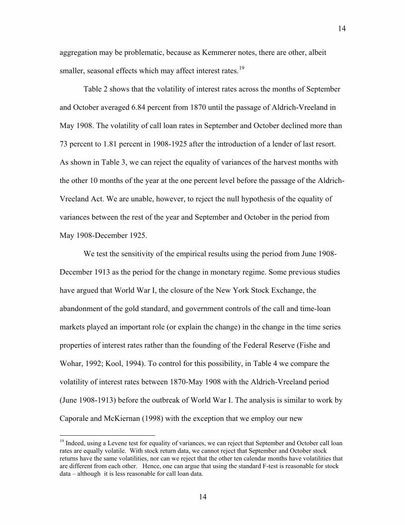
Table 2 shows that the volatility of interest rates across the months of September

and October averaged 6.84 percent from 1870 until the passage of Aldrich-Vreeland in

May 1908. The volatility of call loan rates in September and October declined more than

73 percent to 1.81 percent in 1908-1925 after the introduction of a lender of last resort.

As shown in Table 3, we can reject the equality of variances of the harvest months with

the other 10 months of the year at the one percent level before the passage of the Aldrich-

Vreeland Act. We are unable, however, to reject the null hypothesis of the equality of

variances between the rest of the year and September and October in the period from

May 1908-December 1925.

We test the sensitivity of the empirical results using the period from June 1908-

December 1913 as the period for the change in monetary regime. Some previous studies

have argued that World War I, the closure of the New York Stock Exchange, the

abandonment of the gold standard, and government controls of the call and time-loan

markets played an important role (or explain the change) in the change in the time series

properties of interest rates rather than the founding of the Federal Reserve (Fishe and

Wohar, 1992; Kool, 1994). To control for this possibility, in Table 4 we compare the

volatility of interest rates between 1870-May 1908 with the Aldrich-Vreeland period

(June 1908-1913) before the outbreak of World War I. The analysis is similar to work by

Caporale and McKiernan (1998) with the exception that we employ our new

19 Indeed, using a Levene test for equality of variances, we can reject that September and October call loan rates are equally volatile. With stock return data, we cannot reject that September and October stock returns have the same volatilities, nor can we reject that the other ten calendar months have volatilities that are different from each other. Hence, one can argue that using the standard F-test is reasonable for stock data – although it is less reasonable for call loan data.

14

15

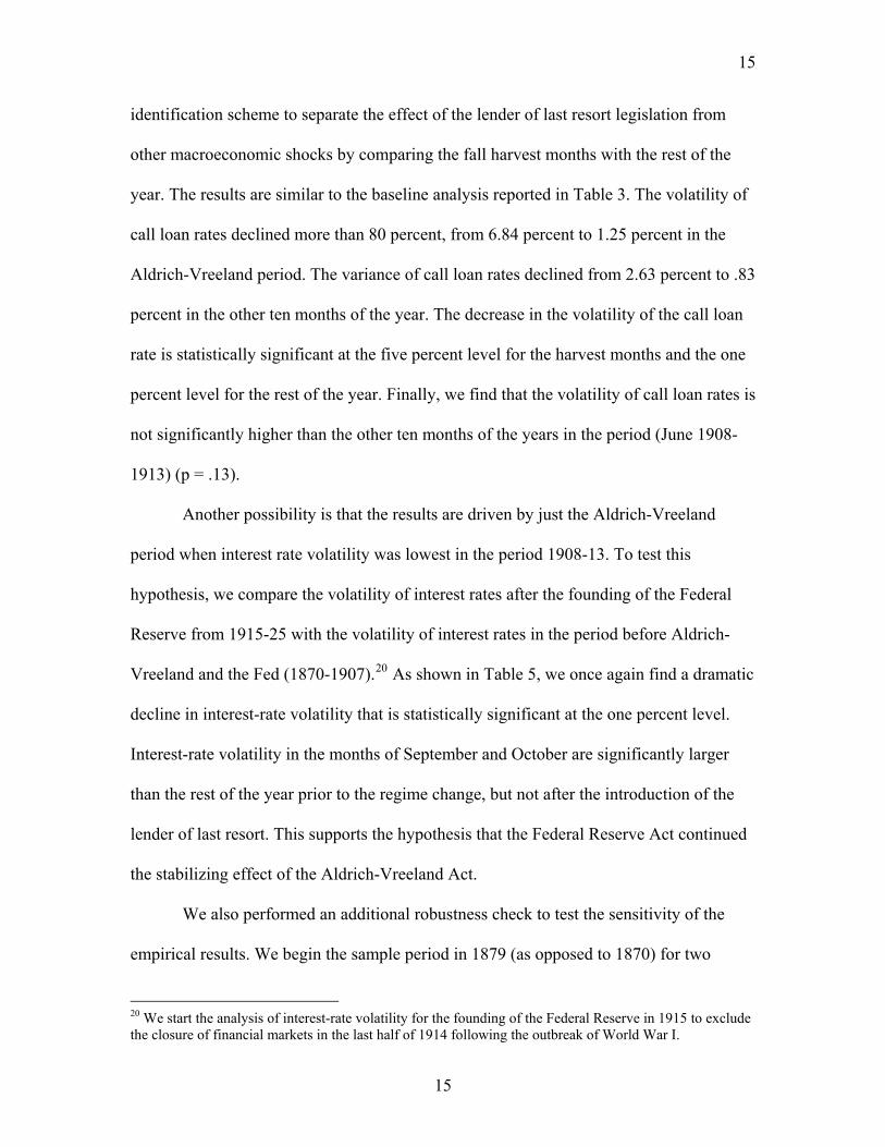
identification scheme to separate the effect of the lender of last resort legislation from

other macroeconomic shocks by comparing the fall harvest months with the rest of the

year. The results are similar to the baseline analysis reported in Table 3. The volatility of

call loan rates declined more than 80 percent, from 6.84 percent to 1.25 percent in the

Aldrich-Vreeland period. The variance of call loan rates declined from 2.63 percent to .83

percent in the other ten months of the year. The decrease in the volatility of the call loan

rate is statistically significant at the five percent level for the harvest months and the one

percent level for the rest of the year. Finally, we find that the volatility of call loan rates is

not significantly higher than the other ten months of the years in the period (June 1908-

1913) (p = .13).

Another possibility is that the results are driven by just the Aldrich-Vreeland

period when interest rate volatility was lowest in the period 1908-13. To test this

hypothesis, we compare the volatility of interest rates after the founding of the Federal

Reserve from 1915-25 with the volatility of interest rates in the period before Aldrich-

Vreeland and the Fed (1870-1907).20 As shown in Table 5, we once again find a dramatic

decline in interest-rate volatility that is statistically significant at the one percent level.

Interest-rate volatility in the months of September and October are significantly larger

than the rest of the year prior to the regime change, but not after the introduction of the

lender of last resort. This supports the hypothesis that the Federal Reserve Act continued

the stabilizing effect of the Aldrich-Vreeland Act.

We also performed an additional robustness check to test the sensitivity of the

empirical results. We begin the sample period in 1879 (as opposed to 1870) for two

20 We start the analysis of interest-rate volatility for the founding of the Federal Reserve in 1915 to exclude the closure of financial markets in the last half of 1914 following the outbreak of World War I.

15

16

reasons: (1) the United States joined the gold standard in 1879 and (2) to exclude the

Panic of 1873 from the empirical analysis which may be driving the empirical results

given that call loan rates increase to more than 60 percent during the crisis. As shown in

Table 6, the basic tenor of the results remains unchanged. Again, we find that interest rate

volatility is significantly higher in September and October than the rest of the year prior

to the monetary regime change. Interest-rate volatility declined from 3.24 percent from

1879-May 1908 to 1.81 percent in the period June 1908-1925 and 1.25 percent from

(June 1908-1913).21 Finally, our results are qualitatively unchanged when we perform

our analyses using commercial paper rates instead of call loan rates.22

One possible shortcoming of the analysis is that the decline in volatility may be

due to a decrease in the seasonality of interest rates. That is, interest rates were higher in

September and October. Other studies have found this to be an important effect of the

founding of the Fed (Miron, 1986; Mankiw, Miron, and Weil, 1987). To test this

hypothesis, we decomposed the decline in time-series volatility into the fraction that can

be explained by a reduction in the variance of interest rates and the portion that can be

explained by a decrease in interest rates. The results are given in Table 7. Bootstrapping

the sample means and variances, we find that decreasing average interest rates without a

corresponding decrease in the variance of those rates cannot explain the observed drop in

volatility (p=0.9979). In contrast, decreasing interest rate variance without altering

average interest rates can explain the observed results (p=0.0005).23

21 Results still hold if the massive call loan rates in 1873 (displayed in figure 6) are excluded from the analysis. 22 See Appendix Table 4 for these results. 23 We thank Peter Rousseau for suggesting this analysis. Additional details on methodology can be found in the Appendix.

16

17

D. Stock Return Volatility

We next examine stock return volatility before and after the monetary regime

change using the equally-weighted GIP Index. Table 8 summarizes the standard deviation

of stock returns in September and October as well as the rest of the year for the period

1870-1925. The standard deviation of stock returns averaged 7.30 percent between 1870-

May 1908 in the months of September and October and 5.80 percent for the rest of the

year. In the lender of last resort period (June 1908-1925), stock volatility declined to 3.83

percent in September and October and 4.68 percent in the other ten months. Volatility

declined by nearly 50 percent in the fall harvest months and more than 19 percent in the

remainder of the year. Table 9 shows that stock return volatility was significantly higher

in the months of September and October relative to the rest of the year before the passage

of the Aldrich-Vreeland and Federal Reserve Acts. After the monetary regime change, we

find that volatility in the fall harvest months was no longer statistically different from the

rest of the year. Consistent with the interest-rate analysis, we also find that the variance

of stock returns significantly declined over the entire year with the biggest decrease

occurring in September and October.

We also conducted a series of robustness checks to test the sensitivity of the

empirical results. Table 10 shows the equality of variance tests for stock returns

comparing the period 1870-May 1908 with the Aldrich-Vreeland period (June 1908-

1913) before the outbreak of World War I. We find that the variance of stock returns was

significantly higher in September and October than the rest of the year before the

monetary regime change. The variance of stock returns was also significantly lower in the

17

18

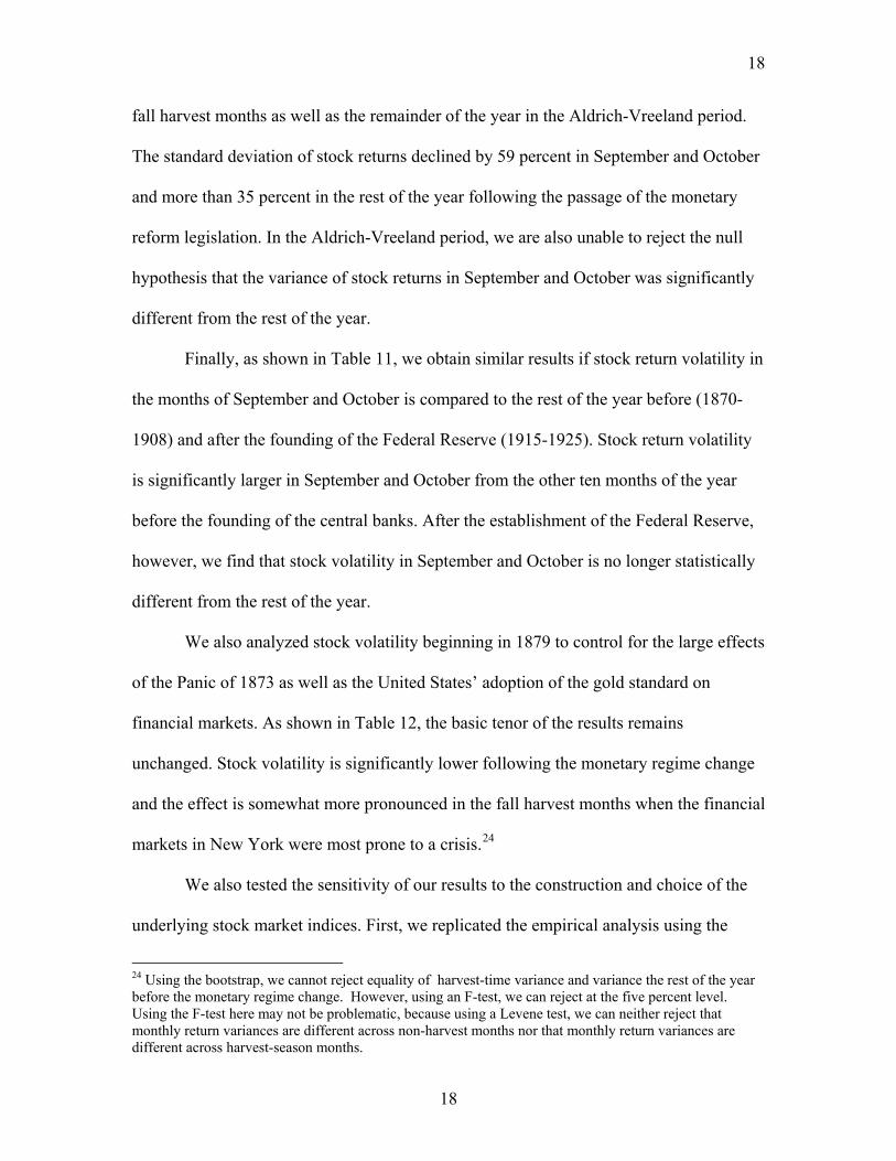
fall harvest months as well as the remainder of the year in the Aldrich-Vreeland period.

The standard deviation of stock returns declined by 59 percent in September and October

and more than 35 percent in the rest of the year following the passage of the monetary

reform legislation. In the Aldrich-Vreeland period, we are also unable to reject the null

hypothesis that the variance of stock returns in September and October was significantly

different from the rest of the year.

Finally, as shown in Table 11, we obtain similar results if stock return volatility in

the months of September and October is compared to the rest of the year before (1870-

1908) and after the founding of the Federal Reserve (1915-1925). Stock return volatility

is significantly larger in September and October from the other ten months of the year

before the founding of the central banks. After the establishment of the Federal Reserve,

however, we find that stock volatility in September and October is no longer statistically

different from the rest of the year.

We also analyzed stock volatility beginning in 1879 to control for the large effects

of the Panic of 1873 as well as the United States’ adoption of the gold standard on

financial markets. As shown in Table 12, the basic tenor of the results remains

unchanged. Stock volatility is significantly lower following the monetary regime change

and the effect is somewhat more pronounced in the fall harvest months when the financial

markets in New York were most prone to a crisis.24

We also tested the sensitivity of our results to the construction and choice of the

underlying stock market indices. First, we replicated the empirical analysis using the

24 Using the bootstrap, we cannot reject equality of harvest-time variance and variance the rest of the year before the monetary regime change. However, using an F-test, we can reject at the five percent level. Using the F-test here may not be problematic, because using a Levene test, we can neither reject that monthly return variances are different across non-harvest months nor that monthly return variances are different across harvest-season months.

18

19

Dow Jones Industrial Average, , which began in 1896 using end-of-month data

collected by Brown et. al. (2008). We also constructed several other market indices using

the GIP data: an equally-weighted monthly return index, , an index of railroad

stocks, , sorting stocks by monthly closing price into the top-third, , middle-third,

, and lowest-third, . This indexing strategy is used as a proxy for both liquidity and

market cap, since historically they have shown a strong correlation.

Dtr

EQtr

RRtr

Btr

Mtr

Str

25 The basic tenor of

the empirical results remains unchanged using the various indices with the exception of

the small firm index. We find that the variability of the small firm index was not

statistically different in the fall harvest season from the other ten months of the year

before the monetary regime change. However, we did find that overall stock volatility for

small firms declined following the monetary policy change.26 We do not view the

empirical results for the small stock index to be very important, however, given that the

small firm index contains many illiquid stocks and constitutes less than three percent of

the market capitalization of the GIP Index.

Finally, we performed the same analysis using the Cowles Index, . In

September and October, stock return volatility across months drops from 3.61 percent

prior to Aldrich-Vreeland to 2.91 percent afterward. As shown in Table 13, the

difference is not statistically significant at conventional levels, however. Further, stock

return volatility in other months actually rises from 3.16 percent prior to Aldrich-

Ctr

25 Though numbers are not reported here, analysis by Weidenmier, Brown, and Mulherin (forthcoming) reveal extremely strong correlation between price and market capitalization during this period. 26 The empirical analysis of small stocks is not surprising for two reasons: (1) as shown in Table 3, the first-order serial correlation of the small stock index, , is 11 percent and (2) the annualized volatility of the index is 37 percent, three times higher than the volatility of our index of high-priced stocks. The high volatility for the small firm index means that it is difficult to conduct hypothesis testing because the standard errors for the index are very large. Detailed results are available from the authors upon request.

Sr

19

20

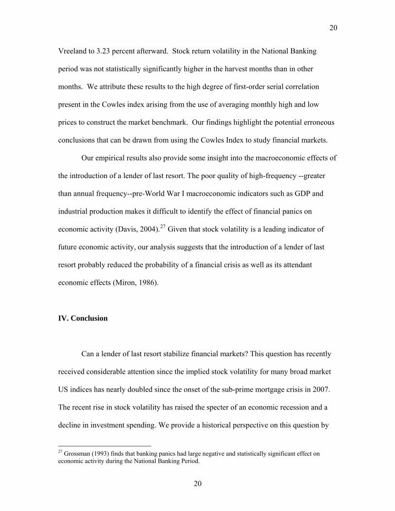
Vreeland to 3.23 percent afterward. Stock return volatility in the National Banking

period was not statistically significantly higher in the harvest months than in other

months. We attribute these results to the high degree of first-order serial correlation

present in the Cowles index arising from the use of averaging monthly high and low

prices to construct the market benchmark. Our findings highlight the potential erroneous

conclusions that can be drawn from using the Cowles Index to study financial markets.

Our empirical results also provide some insight into the macroeconomic effects of

the introduction of a lender of last resort. The poor quality of high-frequency --greater

than annual frequency--pre-World War I macroeconomic indicators such as GDP and

industrial production makes it difficult to identify the effect of financial panics on

economic activity (Davis, 2004).27 Given that stock volatility is a leading indicator of

future economic activity, our analysis suggests that the introduction of a lender of last

resort probably reduced the probability of a financial crisis as well as its attendant

economic effects (Miron, 1986).

IV. Conclusion

Can a lender of last resort stabilize financial markets? This question has recently

received considerable attention since the implied stock volatility for many broad market

US indices has nearly doubled since the onset of the sub-prime mortgage crisis in 2007.

The recent rise in stock volatility has raised the specter of an economic recession and a

decline in investment spending. We provide a historical perspective on this question by

27 Grossman (1993) finds that banking panics had large negative and statistically significant effect on economic activity during the National Banking Period.

20

21

examining the effects of one the most important monetary regime changes in American

history-- the Aldrich-Vreeland Act in 1908 and the creation of the Federal Reserve in

1913--on stock and interest rate volatility.

We introduce a new identification strategy to isolate the effect of the introduction

of a lender of last resort on American financial markets from other macroeconomic

shocks such as World War I, the shutdown of American financial markets from July-

December 1914, and the abandonment of the gold standard. Our identifying strategy is

motivated by the observation that many of the largest financial crises of the National

Banking Period occurred in the months of September and October when the money and

short-term credit markets were relatively illiquid because of the harvest season. We

exploit the seasonal variation in equity and credit markets to identify the effect of the

Aldrich-Vreeland Act and the creation of the Federal Reserve on financial market

volatility.

Using Goetzman, Ibbotson, and Peng’s new comprehensive pre-CRSP database,

we find that the monetary regime change was associated with a dramatic reduction in

financial market volatility. Stock volatility in the months of September and October

declined nearly 50 percent in the Aldrich-Vreeland and Federal Reserve period. Interest-

rate volatility declined more than 70 percent in September and October following the

monetary regime change. Although we find that financial market volatility in September

and October was significantly higher in the pre-Aldrich-Vreeland period than the other 10

months in the year, this was not the case after the introduction of a lender of last resort.

The results provide strong evidence that the introduction of a lender of last resort

stabilized American financial markets.

21

22

The analysis also provides some evidence on the economic effects of a lender of

last resort. The poor quality of macroeconomic indicators such as GDP, investment

spending, and industrial production in the pre-World War II period makes it difficult to

assess the effect of the policy changes on the US economy, although Schwert (1990)

finds that during the period 1889-1925, lagged stock returns do forecast the current level

of real activity. Another problem is that it is difficult to analyze the linkages between the

financial and real sectors given that credit and equity markets are forward looking and

economic data are not. By examining financial market volatility, we gain some insight

into the effects of the introduction of a lender of last resort on the US economy given that

stock volatility is a leading indicator of future investment spending and economic

activity. We interpret our results as strong evidence that the introduction of a lender of

last resort significantly reduced the probability of a financial crisis and its potentially

negative effects on economic activity, especially in the fall harvest months.

Our results have several implications for future studies of financial markets as

well as monetary policy in a time of crisis. First, the findings highlight the potential

problems in using the Cowles Index to test hypotheses in financial economics. Future

research in financial economics may want to revisit the findings of previous studies that

have relied on the Cowles Index to study the behavior of stock returns or stock volatility

over a long period of time. Second, from the perspective of policymakers, liquidity

assistance from a lender of last resort can be very important in preventing a larger

meltdown in financial markets and reducing the probability of a future financial crisis

that can have real economic effects.

22

23

References

Bernanke, B. and M. Gertler. (1989). “Agency Costs, Net Worth, and Business Fluctuations.” American Economic Review 79(1): 14-31.

Bernanke, B. and M. Gertler. (2000). “Asset Price Volatility and Monetary Policy.”

NBER Working Paper #7559. Bordo, M. “The Lender of Last Resort: Some Historical Insights.” NBER Working Paper

#3011.

Brown, W., Mulherin, J., and Weidenmier, M. (forthcoming). “Competing With the NYSE.” Quarterly Journal of Economics.

Caporale, B. and T. Caporale. (2003). “Investigating the Effects of Monetary Regime

Shifts:The Case of the Federal Reserve and the Shrinking Risk Premium.” Economics Letters 80(1): 87-91.

Caporale, T and McKiernan, B. (1998). “Interest Rate Uncertainty and the Founding of

the Federal Reserve.” Journal of Economic History 58(4): 1110-17. Champ, B. (2007a). “The National Banking System: A Brief History.” Federal Reserve

Bank of Cleveland Working Paper. Champ, B. (2007b). “The National Banking System: Empirical Observations.” Federal

Reserve Bank of Cleveland Working Paper. Champ, B. (2007c). “The National Banking System: The National Bank Note Puzzle.”

Federal Reserve Bank of Cleveland Working Paper. Champ, B., and Wallace, N. (2003). “Resolving the National Banking System Note-Issue

Puzzle.” Federal Reserve Bank of Cleveland Working Paper.

Champ, B., Freeman, S., and Weber, W. E. (1999). “Redemption costs and interest rates under the U.S. National Banking System.” Journal of Money, Credit, and Banking 31(3): 568-595.

Champ, B., Smith, B. D., and Williamson, S. D. (1996). “Currency Elasticity and

Banking Panics: Theories and Evidence.” Canadian Journal of Economics 29(4): 828-864.

Clark, T. (1986). “Interest Rate Seasonals and the Federal Reserve.” The Journal of

Political Economy 94(1): 76-125. Davis, J. (2004). “An Annual Index of Industrial Production, 1789-1915.” Quarterly

Journal of Economics 119(4): 1177-1215.

23

24

Davis, J., Hanes, C., and Rhode, R. (2004). “Harvests and Business Cycles in Nineteenth

Century America,” SUNY-Binghamton Working Paper. Fishe, R. P., and Wohar, Mark. (1990). “The Adjustment of Expectations to a Change in

Regime: Comment.” American Economic Review 80(4): 531-551. Friedman, M., & Schwartz, A. J. (1963). A Monetary History of the United States, 1867-

1960. Princeton: Princeton University Press. Goetzmann, W. N., Ibbotson, G. R., and Peng, L. (2001). “A New Historical Database

for The NYSE 1815 To 1925: Performance and Predictability.” Journal of Financial Markets 4(1): 1-32.

Goodhart, C. A. (1969). The New York Money Market and the Finance of Trade, 1900-

1913. Cambridge: Harvard University Press. Grossman, R. (1993). “The Macroeconomic Consequences of Bank Failures under the

National Banking System.” Explorations in Economic History 30: 294-320. Kemmerer, E. W. (1911). “Seasonal Variations in the New York Money Market.”

American Economic Review 1(1): 33-49. Kool, Clemens (1995). “War Finance and Interest Rate Targeting: Regime Changes in

1914-1918.” Explorations in Economic History 32(3): 365-82. Macaulay, F. R. (1938). Some Theoretical Problems Suggested by the Movement of

Interest Rates, Bond Yields and Stock Prices in the United States since 1856. New York: National Bureau of Economic Research.

Mankiw, N. G., and Miron, A. J. (1985). “The Changing Behavior of the Term Structure

of Interest Rates.” NBER Working Paper. Meltzer, A. (2003). A History of the Federal Reserve. Chicago: Chicago University

Press. Miron, A. J., Mankiw, N. G., and Weil, D. N. (1987). “The Adjustment of Expectations

to a Change in Regime: A Study of the Founding of the Federal Reserve.” American Economic Review 77(3): 358-374.

Miron, J. (1986). “Financial Panics, the Seasonality of the Nominal Interest Rate, and the

Founding of the Fed.” American Economic Review 76(1): 125-140. Moen, J. and Tallman, E. (2000). “Clearinghouse Membership and Deposit Contraction

during the Panic of 1907.” Journal of Economic History 60(1): 145-63.

24

25

Piatt, A. A. (1906). “The Influence of Crops Upon Business in America.” Quarterly Journal of Economics , 323-353.

Schwert, G.W. (1989a). “Business Cycles, Financial Crises and Stock Volatility.” Carnegie-Rochester Conference Series on Public Policy 31: 83-125. Schwert, G.W. (1989b). “Why Does Stock Market Volatility Change Over Time?” Journal of Finance 44(5): 1115-1153. Schwert, G.W. (1990). “Stock Returns and Real Activity: A Century of Evidence.” Journal of Finance 45(4): 1237-1257. Shapiro, M.D. (1988). “The Stabilization of the US Economy: Evidence from the Stock Market.” American Economic Review 78(5): 1067-079. Shiller, R. (1992). Market Volatility. Cambridge: MIT Press. Siegel, J. (2002). Stocks for the Long Run: The Definitive Guide to Financial Market Returns and Long-Term Investment Strategies. New York: McGraw Hill. Silber, W. L. (2005). “What Happened to Liquidity When World War I Shut the NYSE?” Journal of Financial Economics 78(3): 685-701. Silber, W. L. (2007a). When Washington Shut Down Wall Street: The Great Financial

Crisis of 1914 and the Origins of America’s Monetary Supremacy. Princeton: Princeton University Press.

Silber, W. L. (2007b). “The Great Financial Crisis of 1914: What can We Learn from

Aldrich-Vreeland Currency?” American Economic Review Paper and Proceedings, 97(2): 285-89.

Sprague, O. M. (1910). A History of Crises under the National Banking System. Washington: U.S. Government Printing Office.

Weber, W. (2000). Federal Reserve Bank of Minneapolis - Bruce Champ. Retrieved

April 20, 2008, frohttp://reserach.mpls.frb.fed.us/research/economists/wewproj.html Working, H. (1960). A Note on the Correlation of First Differences of Averages in a

Random Chain. Econometrica 28: 916-918.

25

26

Table 1 Annualized Mean Monthly Call Loan Rates

(in percent) Month 1870-May 1908 June 1908-1925

January 4.38 3.77

February 3.59 3.88

March 4.30 3.76

April 4.70 3.69

May 3.52 3.67

June 2.95 3.61

26

27

July 2.80 3.63

August 3.22 3.57

September 5.72 3.94

October 5.45 4.35

November 5.04 4.65

December 6.48 4.78

Average 4.35 3.94

Average(non-Sept. & Oct.) 4.10 3.90

Average(Sept. & Oct.) 5.59 4.15

Source: NBER Macro-History Database, Series 13001.

27

28

Table 2 Call Loan Interest Rate Volatility

(in percent) Sample Period Rest of Year September & October

1870-May 1908 2.63 6.84

1879-May 1908 2.36 3.24

June 1908-1913 0.83 1.25

June 1908-1925 1.85 1.81

Table 3 Tests for the Equality of Variance for Call Loans

Full Sample Period (1870-1925) H0: Null Hypothesis Empirical P-value

Harvest Months(1870-May 1908) = Rest of Year(1870-May 1908) 0.0004

Harvest Months(1870-May 1908) = Harvest Months(June 1908-1925)

0.0009

Harvest Months(June 1908-1925) = Rest of Year(June 1908-1925) 0.4009

Rest of Year(1870-May 1908) = Rest of Year(June 1908-1925) 0.0001


Sub-Sample Period (1870-1913) H0: Null Hypothesis Empirical P-value


Harvest Months(1870-May 1908) = Harvest Months(June 1908-1913)

0.0479


28

29


Federal Reserve Sub-Sample Period (1870- May 1908) vs. (1915-1925) H0: Null Hypothesis Empirical P-value

Harvest Months(1870- May 1908) = Harvest Months(1915-1925) 0.0002

Rest of Year(1870- May 1908) = Rest of Year(1915-1925) 0.0033

Rest of Year(1915 – 1925) = Harvest Months(1915 – 1925) 0.3389

Table 6 F-Tests for the Equality of Variance for Call Loans



Harvest Months(1879-May 1908) = Harvest Months(June 1908-1925) 0.0045


Table 7 Tests for the Equality of Variance for Call Loans (Effect of Mean Change)


Harvest Months(1870-May 1908) = Harvest Months(June 1908-1925) (Means the same, but variances different)

0.0005

Harvest Months(1870-May 1908) = Harvest Months(June 1908-1925) (Means different, but variances the same)

0.9979

29

30

Table 8 Standard Deviation of Stock Returns Across Months

(in percent) Sample Period Rest of Year September & October

1870-May 1908 5.80 7.30

1879-May 1908 5.91 6.50

June 1908-1913 3.74 2.97

June 1908-1925 4.68 3.83

Table 9 Tests for the Equality of Variance for Stock Returns







National Banking Period (1870- 1908) vs. Aldrich Vreeland Period (1908-1913) H0: Null Hypothesis Empirical P-value




30

31

31


Federal Reserve Sub-Sample Period (1870- May 1908) vs. (1915-1925) H0: Null Hypothesis Empirical P-value

Harvest Months(1870- May 1908) = Harvest Months(1915-1925) 0.0284

Rest of Year(1870- May 1908) = Rest of Year(1915-1925) 0.0554

Rest of Year(1915 – 1925) = Harvest Months(1915 – 1925) 0.2042






Table 13 Tests for the Equality of Variance for Cowles Index






Figure 1 Monthly Call Loan Interest Rates, 1870-1925

(in percent)

0%

10%

20%

30%

40%

50%

60%

70%

Jan-

70

Jan-

72

Jan-

74

Jan-

76

Jan-

78

Jan-

80

Jan-

82

Jan-

84

Jan-

86

Jan-

88

Jan-

90

Jan-

92

Jan-

94

Jan-

96

Jan-

98

Jan-

00

Jan-

02

Jan-

04

Jan-

06

Jan-

08

Jan-

10

Jan-

12

Jan-

14

Jan-

16

Jan-

18

Jan-

20

Jan-

22

Jan-

24

Monthly Intervals

Passage of Aldrich-Vreeland Act

Figure 2Mean Monthly Call Loan Rates Before and After the Passage of the Aldrich-

Vreeland Act(in percent)

0%

1%

2%

3%

4%

5%

6%

7%

Jan Feb Mar Apr May Jun Jul Aug Sep Oct Nov Dec

1870-May 1908June1908-1925

Figure 3Volatility of Monthly

Call Loan Rates Before & After Aldrich-Vreeland

0%

1%

2%

3%

4%

5%

6%

7%

8%

Rest of Year Sept. & Oct.

Ave

rage

Sta

ndar

d D

evia

tion

of C

ross

-Sec

tiona

Mon

thly

Rat

es

1870- May 19081879- May 1908June 1908-1925June 1908-1913

Figure 4 Volatility of Monthly GIP Index Returns

Before & After Aldrich-Vreeland

0%

1%

2%

3%

4%

5%

6%

7%

8%

Rest of Year Sept. & Oct.

Ave

rage

Sta

ndar

d D

evia

tion

of C

ross

-Sec

tiona

l Mon

thly

Ret

urn

1870- May 1908

1879- May 1908

June 1908-1925

June 1908-1913

Appendix

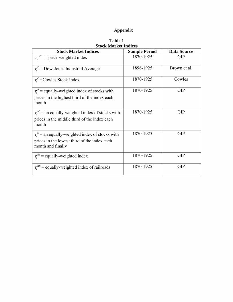
Table 1 Stock Market Indices

Stock Market Indices Sample Period Data Source Wt

tr = price-weighted index 1870-1925 GIP

Dtr = Dow-Jones Industrial Average 1896-1925 Brown et al.

Ctr =Cowles Stock Index 1870-1925 Cowles

Btr = equally-weighted index of stocks with

prices in the highest third of the index each month

1870-1925 GIP

Mtr = an equally-weighted index of stocks with

prices in the middle third of the index each month

1870-1925 GIP

Str = an equally-weighted index of stocks with

prices in the lowest third of the index each month and finally

1870-1925 GIP

Eqtr = equally-weighted index 1870-1925 GIP

RRtr = equally-weighted index of railroads 1870-1925 GIP

Table 2 Correlation of Monthly Returns for Various Stock Market Indices

Wttr D

tr Ctr B

tr Mtr S

tr Eqtr RR

tr

Wttr 1.00

Dtr 0.72 1.00

Ctr 0.66 0.67 1.00

Btr 0.92 0.71 0.61 1.00

Mtr 0.92 0.70 0.60 0.77 1.00

Str 0.81 0.65 0.59 0.63 0.77 1.00

Eqtr 0.94 0.74 0.65 0.81 0.91 0.95 1.00

RRtr 0.88 0.64 0.61 0.76 0.86 0.92 0.96 1.00

Table 3 Annualized Volatility and Serial Correlation

of Monthly Index Returns Wt

tr Dtr C

tr Btr M

tr Str Eq

tr RRtr

σ 0.14 0.20 0.11 0.11 0.20 0.37 0.20 0.23

ρ 0.06 0.06 0.29 0.02 0.06 0.11 0.10 0.08

Notes: σ, is the annualized standard deviation of monthly index returns; ρ is the serial correlation of monthly index returns.

Table 4 Tests for the Equality of Variance for Commercial Paper






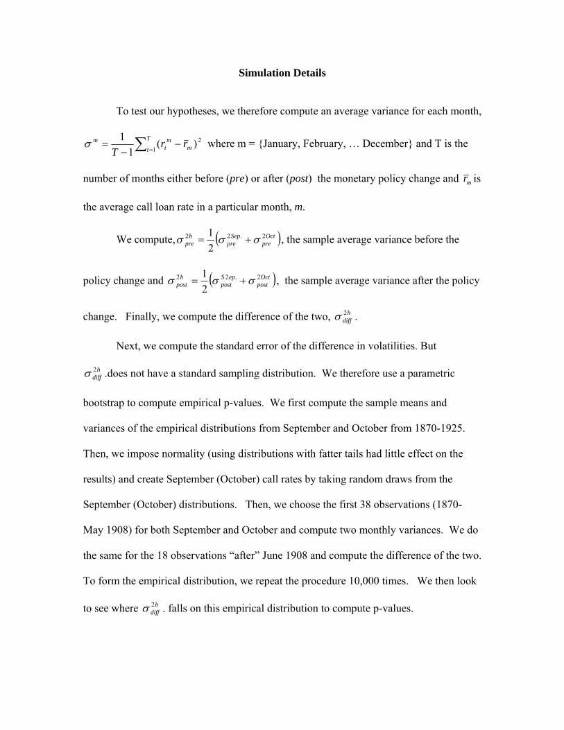
Simulation Details

To test our hypotheses, we therefore compute an average variance for each month,

∑ =−

−=

T

t mm

tm rr

T 12)(

11σ where m = {January, February, … December} and T is the

number of months either before (pre) or after (post) the monetary policy change and mr is

the average call loan rate in a particular month, m.

We compute, ( Octpre

Seppre

hpre

2.22

21 σσσ += ), the sample average variance before the

policy change and ( Octpost

epSpost

hpost

2.22

21 σσσ += ), the sample average variance after the policy

change. Finally, we compute the difference of the two, . hdiff2σ

Next, we compute the standard error of the difference in volatilities. But

.does not have a standard sampling distribution. We therefore use a parametric

bootstrap to compute empirical p-values. We first compute the sample means and

variances of the empirical distributions from September and October from 1870-1925.

Then, we impose normality (using distributions with fatter tails had little effect on the

results) and create September (October) call rates by taking random draws from the

September (October) distributions. Then, we choose the first 38 observations (1870-

May 1908) for both September and October and compute two monthly variances. We do

the same for the 18 observations “after” June 1908 and compute the difference of the two.

To form the empirical distribution, we repeat the procedure 10,000 times. We then look

to see where . falls on this empirical distribution to compute p-values.

hdiff2σ

hdiff2σ

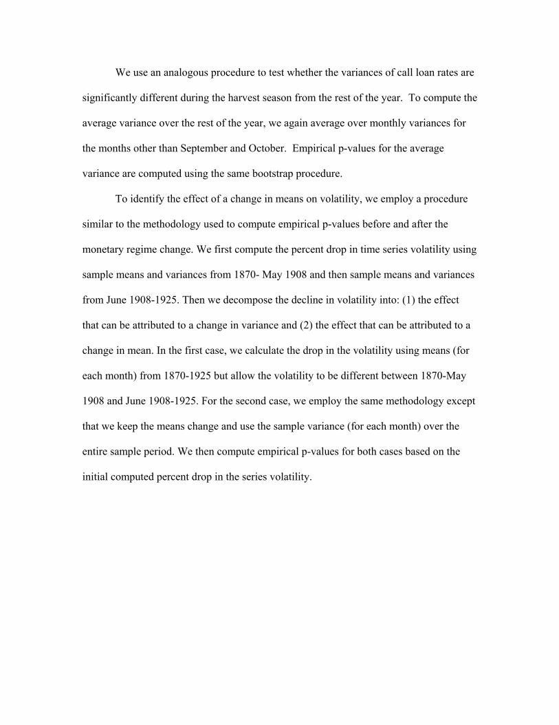
We use an analogous procedure to test whether the variances of call loan rates are

significantly different during the harvest season from the rest of the year. To compute the

average variance over the rest of the year, we again average over monthly variances for

the months other than September and October. Empirical p-values for the average

variance are computed using the same bootstrap procedure.

To identify the effect of a change in means on volatility, we employ a procedure

similar to the methodology used to compute empirical p-values before and after the

monetary regime change. We first compute the percent drop in time series volatility using

sample means and variances from 1870- May 1908 and then sample means and variances

from June 1908-1925. Then we decompose the decline in volatility into: (1) the effect

that can be attributed to a change in variance and (2) the effect that can be attributed to a

change in mean. In the first case, we calculate the drop in the volatility using means (for

each month) from 1870-1925 but allow the volatility to be different between 1870-May

1908 and June 1908-1925. For the second case, we employ the same methodology except

that we keep the means change and use the sample variance (for each month) over the

entire sample period. We then compute empirical p-values for both cases based on the

initial computed percent drop in the series volatility.

Can a Lender of Last Resort Stabilize Financial Markets

Documents

Transcript of Can a Lender of Last Resort Stabilize Financial Markets