NBER WORKING PAPER SERIES

ECONOMIC PREPARATION FOR RETIREMENT

Michael D. HurdSusann Rohwedder

Working Paper 17203http://www.nber.org/papers/w17203

NATIONAL BUREAU OF ECONOMIC RESEARCH1050 Massachusetts Avenue

Cambridge, MA 02138July 2011

We gratefully acknowledge research support from the Social Security Administration via the MichiganRetirement Research Center (UM06-03and UM09-08), from the Department of Labor (J-9-P-2-0033),and from the National Institute on Aging (P01AG08291 and P01AG022481). We thank Joanna Carrollfor excellent programming assistance. The views expressed herein are those of the authors and donot necessarily reflect the views of the National Bureau of Economic Research.

NBER working papers are circulated for discussion and comment purposes. They have not been peer-reviewed or been subject to the review by the NBER Board of Directors that accompanies officialNBER publications.

© 2011 by Michael D. Hurd and Susann Rohwedder. All rights reserved. Short sections of text, notto exceed two paragraphs, may be quoted without explicit permission provided that full credit, including© notice, is given to the source.

Economic Preparation for RetirementMichael D. Hurd and Susann RohwedderNBER Working Paper No. 17203July 2011JEL No. E21,J14,J26

ABSTRACT

We define and estimate measures of economic preparation for retirement based on a complete inventoryof economic resources while taking into account the risk of living to advanced old age and the riskof high out-of-pocket spending for health care services. We ask whether, in a sample of 66–69 year-olds,observed economic resources could support with high probability a life-cycle consumption path anchoredat the initial level of consumption until the end of life. We account for taxes, widowing, differentialmortality and out-of-pocket health spending risk. We find that 71% of persons in our target age groupare adequately prepared according to our definitions, but there is substantial variation by observablecharacteristics: 80% of married persons are adequately prepared compared with just 55% of singlepersons. We estimate that a reduction in Social Security benefits of 30 percent would reduce the fractionadequately prepared by 7.8 percentage points among married persons and by as much as 10.7 percentagepoints among single persons.

Michael D. HurdRAND Corporation1776 Main StreetSanta Monica, CA 90407and NBERmhurd@rand.org

Susann RohwedderRAND1776 Main StreetP.O. Box 2138Santa Monica, CA 90407susannr@rand.org

1

1. Introduction

The most common metric for assessing the adequacy of economic preparation for retirement is the income replacement rate, the ratio of income after retirement to income before retirement. This metric is usually applied without regard to family circumstances or /to the complete portfolio of economic resources, particularly wealth. Thus, it is stated that a single person or a couple is adequately prepared if their post-retirement income is in some fixed ratio (such as 80%) to their pre-retirement income. However both economic theory and common sense say that someone is adequately prepared if she is able to maintain her level of economic well-being, which is not the same as maintaining her level of income or some fixed proportion of income because of the accumulation and decumulation of wealth.

Consumption is a better measure of well-being or utility than the level of income at some particular point in time. But, the relationship of consumption after retirement to consumption before retirement is not at all well measured by the relationship of income after retirement to income before retirement, which is the income replacement ratio. Consumption before retirement will typically be substantially less than income before retirement because of taxes (and Social Security contributions) and work-related expenses, but most importantly because of saving for retirement. Consumption after retirement will typically be greater than income because of the ability to spend out of saving. Furthermore, many retired households pay little or no taxes and make no Social Security contributions. The implication is that income could change by a great deal at retirement, yet consumption could be maintained.1

The overall goal of this paper is to assess economic preparation for retirement in a way that addresses many of the deficiencies of the income replacement rate concept. We will find whether shortly after retirement households have the financial resources needed to finance a consumption plan from retirement through the end of life. The consumption plan begins at an observed starting value for each household and follows a path whose shape is determined by observed consumption change with age in panel data. We classify a single person as being adequately prepared if he or she dies with positive bequeathable wealth. A married person is adequately prepared if he or she dies with positive wealth where he or she may die as a married person or as a surviving spouse.

Because the age of death is unknown and because wealth is not completely annuitized, someone who dies unexpectedly early may have been adequately prepared ex post, yet someone who survives to extreme old age will not have been adequately prepared ex post. To account for this randomness we find via simulation the fraction of times ex post a household was adequately prepared.

Economic resources are a combination of post-retirement income, housing wealth and nonhousing wealth. The estimations and simulations account for mortality risk, and, in the case of couples, the lifetime of the couple and the subsequent loss of returns-to-scale in consumption at the death of the first spouse. They recognize that consumption need not be constant with age. They incorporate the risk of large out-of-pocket spending on 1 An additional complicating factor is whether individuals have had children: if so, they will want to spend relatively more of their lifetime income during their working lives and thus will reach retirement with less wealth than someone who did not have children.

2

health care. We account for taxes which for some households substantially reduce resources available for consumption.

Our main result is that about 70% of individuals age 66-69 are adequately financially prepared for retirement. However, some individuals identified by education, sex and marital status are not financially prepared, most notably single females who lack a high school education: just 29% of that group is adequately prepared.

2. Data

Our analyses are based on data from the Health and Retirement Study (HRS) and data from the Consumption and Activities Mail Survey (CAMS). The HRS is a biennial panel. Its first wave was conducted in 1992. The target population was the cohorts born in 1931-1941 (Juster and Suzman, 1995). Additional cohorts were added in 1993 and 1998 so that in 1998 it represented the population from the cohorts of 1947 or earlier. In 2004 more new cohorts were added making the HRS representative of the population 51 or older. The HRS is very rich in content. In this study we take advantage of the detailed information on economic resources, out-of-pocket medical expenditures, and longitudinal information on survival.

The CAMS is a supplemental survey to the HRS that is administered to a random subsample of HRS households. One of its main objectives is to elicit total household spending over the preceding 12 months which can be linked to the rich information collected in the HRS core survey on the same individuals and households. The first wave of CAMS was collected in the Fall of 2001, and longitudinal follow-up surveys have been conducted every two years since then. When HRS inducts a refresher cohort into the survey, a random-subsample of households that are part of the refresher group are also inducted into the CAMS. In this study we use data on household spending from the first four waves of CAMS, spanning the period from 2001 through 2007.2 In the first two waves the unit response rate in CAMS was in the high 70s and it was 72 percent in waves 3 and 4. This yields spending data for just under 3,700 HRS households on average in each wave of CAMS.

With the CAMS, the HRS is the only general-purpose survey to attempt collecting a detailed measure of total spending. The fact that CAMS is longitudinal and that the spending data can be linked to the rich background information in the HRS core survey make the data unique. While the HRS cannot afford the level of detail asked about in the Consumer Expenditure Survey (CEX), which is the survey in the U.S. that collects the most detailed and comprehensive information on total spending, CAMS nevertheless is notable for a number of design features that enhance data quality of the spending information.3 These features have generated high item response rates so that relatively little information needs to be imputed to arrive at a measure of total spending for all households.

2 We do not use data from CAMS 2009 because of the financial crisis. Observed consumption in CAMS 2009 was unusually low and that low level is unlikely to be maintained in the future. Anchoring baseline consumption to that temporarily low level would under-estimate actual future spending and, hence, over-estimate economic preparation for retirement. 3 See data appendix for details.

3

A natural validation exercise for the spending data in CAMS is to compare them to the CEX. As we show in Hurd and Rohwedder (2009a) the totals are almost identical among those 55-64. At older ages the CEX shows lower spending than the CAMS, implying a much higher rate of saving for the older population than is consistent with actual rates of change in wealth as observed in HRS panel data. We therefore believe that the statistics from CAMS for the older population have greater validity.4

3. Methods

Our approach relies on simulating consumption paths over the remaining lifetime for a sample of households observed shortly after retirement. We construct life-cycle consumption paths for each household. Whereas a model based on a particular utility function would specify that the slope of the consumption path depends on the interest rate, the subjective time-rate of discount, mortality risk and utility function parameters, we estimate these slopes directly from the data. Thus our estimations use the framework of lifetime utility maximization but they are essentially nonparametric in that we allow the consumption path to be determined directly by the data.

We estimate the consumption trajectories from the initial level of consumption near retirement, which we observe directly in the CAMS data, and observed panel transitions in consumption in CAMS waves 1 to 2, 2 to 3, and 3 to 4 (three transitions). Economic resources at retirement consist of bequeathable wealth and annuities (Social Security benefits, DB pensions benefits and actual annuities). We ask: can the resources support the projected consumption path? Because lifetime is uncertain, and wealth is not typically annuitized, we perform multiple simulations making random draws from mortality tables. We find whether the resources will sustain the path at least until advanced old age where the probability of survival is small. If that is the case, the household will not have under saved ex ante. We investigate whether any shortfalls in resources are large or small by finding the fraction of the sample that would have to reduce consumption by a large percentage to meet the adequacy criterion of being able to finance consumption to advanced old age.

We account for consumption of health care services on average in the CAMS data. This category of consumption is part of the CAMS measurement; consequently, it helps us determine a single person’s initial total level of consumption and the rate of change in consumption with age. If there were no spending risk, out-of-pocket spending for health care would need no further treatment. However, because of spending risk, a single person’s actual consumption of health care services will differ from the average level by a spending shock that has an expected value of zero, but which could be quite large. We construct that shock from HRS data on out-of-pocket spending for health care services.

We do these calculations of the consumption trajectory modified by simulated health care spending shocks for each single person in our CAMS sample who is in his or her early retirement years.

4 Panel wealth change shows slowly declining wealth among couples after age 70. Among single persons, wealth declines after age 70 but at a greater rate. CEX spending when combined with HRS after-tax income would, in contradiction, predict steadily increasing wealth for couples and too little wealth decline among single persons.

4

For couples the basic method is similar. However, the consumption path followed while both spouses survive will differ from the consumption path of single persons, so it is separately estimated from the CAMS data. The couple will follow that consumption path as long as both spouses survive, and then the surviving spouse will switch to the consumption path of a single person. The shape of the single’s path is estimated as described above, but the level of consumption by the surviving spouse will depend on returns-to-scale in consumption by the couple. At the death of the first spouse, the surviving spouse reduces consumption to the level specified by the returns-to-scale parameter. We assume a returns-to-scale parameter that is consistent with the literature and with practice. For example, the poverty line specifies that a couple with 1.26 times the income of a single person who is at the poverty line will also be at the poverty line. This implies that consumption by the surviving spouse should be 79% of consumption by the couple to equate effective consumption. Knowing the consumption path of the surviving spouse we find the expected present value of consumption for the lifetime of the couple and surviving spouse.

We assess adequacy of retirement resources in three ways. First, we compare population averages of the expected present value of consumption with average resources at retirement to find whether the cohort can finance the expected consumption path. Second, we move from the cohort level to the household level to determine the fraction of households that can finance with high probability their expected consumption path. Third we find by how much a household would have to adjust consumption to keep the chances of running out of wealth towards the end of the life cycle small.

4. Model for singles

In this section we develop the ideas discussed previously more formally. Suppose a single person retires at age R . Call that 0t . He or she retires with real annuity 0S and

nominal annuity 0P , the inflation rate is f , and the nominal interest rate F , which

implies a real interest rate r F f . Then the real annuity at some later time t is

00 (1 )t t

PA S

f

. When the only source of uncertainty is mortality risk (and ignoring

any bequest motive), according to the lifecycle model a single person will choose optimal consumption to satisfy

(1) ln 1

( )tt

t

d cr h

dt

as long as bequeathable wealth is positive, where t is local risk aversion (which in

general need not be constant), r is the fixed real interest rate, is the subjective time

rate of discount, and th is mortality risk. Because th is approximately exponential, at

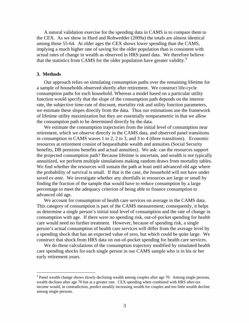
some (relatively young) age consumption will decline with age. The optimal consumption level will be determined by adjusting the consumption path so that at the age when consumption has declined to equal annuity income, age T , bequeathable wealth is zero. At that point consumption will not drop further: it will equal annuities at all subsequent ages. Figure 1 has an example of an optimal path. Initial consumption is 100, initial wealth is 700 (right scale), annuities are 40. The consumption path is determined by

5

equation (1) for the values 0.01, 0.01, and 1.3tr . Mortality risk is for men

from the year 2000 life table. The area under the consumption path but above the annuity path equals initial bequeathable wealth and consumption equals annuities at age 86T when wealth becomes zero.

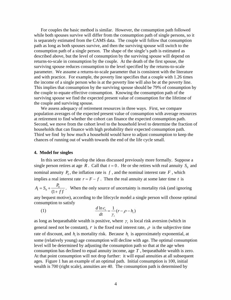
Figure 2 shows the consumption path that is also determined by equation (1), but where initial consumption is 110. Wealth reaches zero at age 78 but consumption at that age is 76 so the lifetime budget constraint requires a discontinuous drop in consumption to 40, which is not optimal. Conditional on survival to at least 79, the single person under saved, or equivalently, over consumed at age 65.

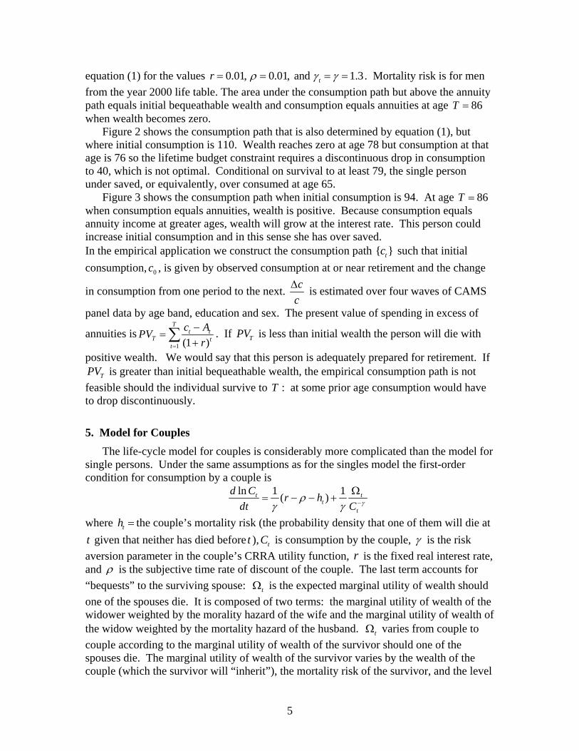
Figure 3 shows the consumption path when initial consumption is 94. At age 86T when consumption equals annuities, wealth is positive. Because consumption equals annuity income at greater ages, wealth will grow at the interest rate. This person could increase initial consumption and in this sense she has over saved. In the empirical application we construct the consumption path { }tc such that initial

consumption, 0c , is given by observed consumption at or near retirement and the change

in consumption from one period to the next. c

c

is estimated over four waves of CAMS

panel data by age band, education and sex. The present value of spending in excess of

annuities is1 (1 )

Tt t

T tt

c APV

r

. If TPV is less than initial wealth the person will die with

positive wealth. We would say that this person is adequately prepared for retirement. If

TPV is greater than initial bequeathable wealth, the empirical consumption path is not

feasible should the individual survive to T : at some prior age consumption would have to drop discontinuously.

5. Model for Couples

The life-cycle model for couples is considerably more complicated than the model for single persons. Under the same assumptions as for the singles model the first-order condition for consumption by a couple is

ln 1 1( )t t

tt

d Cr h

dt C

where th the couple’s mortality risk (the probability density that one of them will die at

t given that neither has died before t ), tC is consumption by the couple, is the risk

aversion parameter in the couple’s CRRA utility function, r is the fixed real interest rate, and is the subjective time rate of discount of the couple. The last term accounts for

“bequests” to the surviving spouse: t is the expected marginal utility of wealth should

one of the spouses die. It is composed of two terms: the marginal utility of wealth of the widower weighted by the morality hazard of the wife and the marginal utility of wealth of the widow weighted by the mortality hazard of the husband. t varies from couple to

couple according to the marginal utility of wealth of the survivor should one of the spouses die. The marginal utility of wealth of the survivor varies by the wealth of the couple (which the survivor will “inherit”), the mortality risk of the survivor, and the level

6

of pension and Social Security benefits that the survivor will have. Predictions about the slope and level of the consumption path are complex because of t . But consumption

should decline if both spouses are old because the marginal utility of wealth will be small for an old surviving spouse. The slope of the consumption path should be greater algebraically (flatter) when one spouse is young because the marginal utility of wealth is large for a young spouse.

To find the predicted consumption path of a couple we begin with 0C , which is

observed consumption by a couple at baseline. Then we project consumption to the next period by 1 (1 )t t tC C G where tG is the annual growth rate of consumption by

couples. We estimate tG by age and education bands between waves 1 and 2, 2 and 3,

and 3 and 4 of CAMS in a non-parametric manner directly from the spending data, just as we did for singles. The associated wealth path is 1 (1 )t t t tW W r C A where r is an

assumed real rate of interest. The couples model differs from the singles model in that one spouse will die before the other and the surviving spouse will continue to consume, but the consumption level will change according to returns-to-scale. Suppose the husband dies. Then the widow will “inherit” the wealth of the couple, an annuity which is some fraction of tA , and a consumption level that reflects returns-to-scale. According

to the poverty line, the widow would need 1/1.26 = 0.794 of the consumption of the couple; according to scaling of the wife’s and widow’s benefits in Social Security, the widow would need 1/1.5 = 0.667. From that point on the widow will follow the singles model taking as initial conditions the inherited wealth, the reduced annuities and the reduced consumption level.

Figure 4 has an example under the assumption that both spouses are initially 65 and that the husband dies at age 80. Initial consumption is 100 and initial wealth is 925. Prior to age 80 consumption by the couple follows 1 (1 )t t tC C G . Consumption

declines when the husband dies because of returns-to-scale, and then it follows the path of singles. In the case shown, the couple and surviving spouse could just exactly afford the initial consumption. Should the widow survive to 91 or beyond, wealth would be exhausted.

If initial consumption were greater than 100 the surviving spouse would be forced to reduce consumption discontinuously should that spouse survive to age 90. If initial consumption were less than 100 the surviving spouse would die with positive wealth.

The foregoing assumes widowing at 80, but we implement random widowing. Take the same couple where both are initially 65. Randomly choose whether both, one or neither spouse survives with probabilities given by life table survival hazards. If both survive we continue calculating the couple’s consumption and wealth path. If the husband dies, we switch to the widow’s consumption path and apply the estimated consumption growth rates of a single female. We find the expected present value of spending in excess of annuities. If the wife dies we perform the same calculation, except that we use the rate of change in consumption estimated for single males. If both die, we stop the calculations.

The outcomes of one simulation are: Did the household die with positive wealth? If so, how much compared with initial wealth? If not, what is the wealth shortfall?

7

By repeating the simulations a number of times for the same household we can find the probability that the household will die with positive wealth or negative wealth and the distribution of those excesses or shortfalls in wealth.

6. Inputs into simulations

Differential mortality A large literature on the gradient between socioeconomic status (SES) and health

documents that individuals with high SES such as high education live longer than those with low SES (Kitagawa and Hauser, 1973; Marmot et al. 1991; Adams et al. 2003). Because households are not fully annuitized, long-lived households have to be prepared to finance consumption over a longer remaining time horizon. We take this into account in our simulations by applying survival probabilities that differentiate by education as well as by age, sex and marital status.

We obtain our estimates of differential mortality based on eight waves of HRS data spanning the years 1992 to 2006. We estimate the probability of survival to time t+1 conditional on being alive at time t, pooling the seven transitions we observe in the HRS. The logit model yields the estimates shown in Table 1 for males and females as a function of age, marital status and education. For single males the odds of survival for college graduates between waves is 44% higher than the odds of survival for high school dropouts. For both men and women the survival odds increase in education, and for both there is a substantial interaction between completing college and being married.

From these estimates we construct survival curves by sex, marital status and education and normalize these to life tables so that the average survival probability given age and sex equals that given in the life tables. Figure 5 has examples of the estimated survival curves for females. A single female lacking a high school education has a 50% chance of surviving to age 80 while a single female with a college education has a 50% change of surviving to age 84. For married women the difference by education is considerably larger: the age at which survival chances fall below 50% is about 10 years greater among women with a college education than among women lacking a high school degree. These survival differences translate into large differences in life expectancy. For example, married men with a college degree have a life expectancy that is 39% greater than single men who lack a high school degree. Such long-lived men need correspondingly greater bequeathable wealth to finance their retirement years.

Figure 6 has similar survival curves for males. The survival chances for males are lower than for females, but the patterns by education and by marital status are similar.

8

Estimation of consumption paths Because survival differs by age, sex and education the slope of the consumption path

should vary by those characteristics according to equation (1). Therefore we estimate the model

(2) 1t ti j k

t

c cu

c

where i indicates the age category, j indicates the education category and k indicates sex. We have four education categories: less than high school, high school, some college and college graduate. For singles we have five age categories 65-69, 70-74, 75-79, 80-84 and 85 or over. We observed 2,037 consumption transitions among singles 65 or older between the four waves of CAMS. For couples we have just four age categories because of small sample size in the top age category. In addition we entered categorical variables for the age of the spouse. We observed 4,593 consumption transitions among couples where both spouses were 62 or older and at least one spouse was 66 – 69. We estimated by median regression because observation error on consumption produces large outliers in the left-hand variable which makes OLS estimates unreliable. We restricted the sample to those with observed positive wealth because consumption change cannot be freely chosen if a household has no wealth.

Table 2 shows the predicted one-year change in consumption by single persons based on equation (2). It is notable that almost all the changes are negative indicating reductions in consumption with age. Table 3 has similar results for married persons. It has a separate panel for couples where the husband is older than the wife by five years or more because theory predicts the slope of the consumption path will be algebraically larger when the wife is young. In the estimation that turns out not to be the case: for example, when the husband is 65-69 and the wife’s age differs from the husband’s by less than five years, the slope is -0.86 (less than high school education), but when the wife’s age differs by five years or more the slope is -2.31. A possible explanation might be that households with a large age difference between spouses differ in some other ways from other households. The prediction from theory assumes that all else is held the same except the age difference.

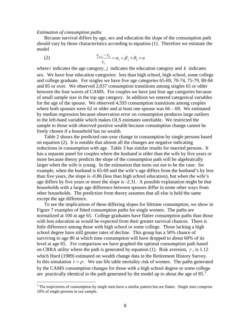
To see the implications of these differing slopes for lifetime consumption, we show in Figure 7 examples of fitted consumption paths for single women. The paths are normalized at 100 at age 65. College graduates have flatter consumption paths than those with less education as would be expected from their greater survival chances. There is little difference among those with high school or some college. Those lacking a high school degree have still greater rates of decline. This group has a 50% chance of surviving to age 80 at which time consumption will have dropped to about 60% of its level at age 65. For comparison we have graphed the optimal consumption path based on CRRA utility where the path is generated by equation (1). Risk aversion, , is 1.12 which Hurd (1989) estimated on wealth change data in the Retirement History Survey. In this simulation r . We use life table mortality risk of women. The paths generated by the CAMS consumption changes for those with a high school degree or some college are practically identical to the path generated by the model up to about the age of 85.5

5 The trajectories of consumption by single men have a similar pattern but are flatter. Single men comprise 18% of single persons in our sample.

9

Figure 8 shows consumption paths of couples where both spouses are the same age. The most obvious difference from the consumption paths of single women is that consumption by couples shows less decline. This is to be expected because the couple has a strong desire to leave wealth to a surviving spouse as reflected in substantial marginal utility of wealth to the surviving spouse. There is little difference in the paths by education.6 Because of the high mortality risk of the couple the most relevant part of the consumption path is up to about age 80. Over this age range consumption declines slowly to about 80% of initial consumption. Future Earnings

In our analytical sample, 24% of 66-69 year old single persons and 23% of married persons are working for pay at baseline. Among married persons those still working are mostly younger spouses. To forecast the future earnings of workers we first predict the probability of working for pay in the next period, conditional on working in the current period. We obtain these predictions from panel data estimations regressing working for pay in the HRS on covariates, including age, sex, marital status and education. We then multiply this probability of working with the respondent’s observed baseline earnings adjusted for earnings growth. Earnings growth by gender and marital status is also estimated on HRS panel data among respondents of the relevant age and with positive earnings in adjacent survey waves. See the Data Appendix for further details.

For those who are not working for pay at baseline we assume that they will not work in the future.

Taxes

Taxes influence economic preparation for retirement via four routes. The first is federal and state tax paid on ordinary income such as earnings, capital income and pension income. The second is Social Security contributions paid on earnings. The third is that Social Security income is only partially counted as taxable income and the fraction depends on the level of other taxable income and on the amount of Social Security income. The fourth is that withdrawals from tax-advantaged accounts such as IRAs are taxed and minimum withdrawals become mandatory at age 70 ½. We have accounted for these taxes in a somewhat simplified manner, which, nonetheless addresses all of these elements.7 See the Data Appendix for further details.

Because low income groups pay very little, if any, taxes in retirement, accounting for taxes for them has little impact on the assessment of whether the household is economically prepared for retirement. For example, the median tax rate among those in the lowest annuity income quartile (pension plus Social Security) is zero, and it is just 1% in the second annuity income quartile. In addition those who pay some income tax often pay no tax at all on Social Security benefits. However, among high-income groups the situation is very different. They tend to have sizeable pre-tax retirement assets (IRAs) and they are most likely to have 85% of their Social Security benefits taxed. As a result taking into account the effect of taxation is likely to have a greater effect on economic

6 Education is the education of the respondent to the CAMS survey 7 We use standard deductions and estimate the relationship between federal and state income taxes for each household based on the NBER tax calculator, TAXSIM (see Feenberg and Coutts, 1993). We use this relationship to estimate state taxes.

10

preparation for retirement for those with more education than for those with less education.

Housing

Older households tend to retain their housing wealth, or more precisely their primary residence, until advanced old age (Venti and Wise, 2004). In terms of financing spending in retirement it appears that housing wealth is often not used until other assets are exhausted. To approximately replicate these patterns we separate housing wealth held in the primary residence from other assets. We assume that this form of housing wealth is not depleted until all other wealth has been drawn down. This matters for taxation, because it requires that IRA balances are withdrawn and subject to taxation before housing equity is accessed. We assume that housing wealth appreciates at a real rate of return of 2.5 percent which is approximately the rate observed from 1985-2006.8 We assume that capital gains in housing accumulate tax free which is the case for the great majority of households, because of the large federal tax exemption ($500,000 lifetime capital gains on primary residence per person) that most people would not exhaust.

Health care spending risk

To account for health care spending risk we draw from the distribution of out-of-pocket health care spending in HRS 2008. We use that year for two reasons. When we compared the level and distribution of out-of-pocket spending for health care in HRS 2004 with similar measures in the Medical Expenditure Panel Survey (MEPS) and the Medicare Current Beneficiary Survey (MCBS) we found that mean out-of-pocket spending in the HRS was about 60% greater than in the MCBS or MEPS (which were similar); yet, HRS medians were practically the same as in MCBS and in MEPS (Hurd and Rohwedder, 2009b). The discrepancy in means is due to some very large values in HRS. For example, the 99th percentile of spending in 2004 HRS was $24,600 expressed in 2003 prices. The 99th percentile in the 2003 MCBS was $11,400 and $9,300 in the 2003 MEPS. Thus the risk of out-of-pocket spending for health care is substantially greater in HRS than in MCBS or in MEPS. We determined that the main source of the difference is in the measurement of spending for prescription drugs. The HRS modified in 2006 the questions about spending on prescription drugs which brought HRS back in line with MEPS and MCBS.9

The second reason we use HRS 2008 is the introduction of Medicare Part D in 2006 which reduced the risk of large out-of-pocket spending for some retirees. This reduction should have an impact on economic preparation for retirement which we want to take into account.

Serial correlation in out-of-pocket spending for health care

People who have chronic conditions are likely to have greater than average spending on heath care each year, which induces serial correlation in out-of-pocket spending. Serial correlation increases the likelihood that someone will have several successive

8 Based on the Federal Housing Finance Agency quarterly house price index adjusted by the CPI. http://www.fhfa.gov/Default.aspx?Page=87 accessed 6/17/2011 9 See Hurd and Rohwedder (2009b) for further details

11

years of high spending, increasing the risk of not being adequately economically prepared for retirement.

To account for serial correlation at the household level we estimate a model of out-of-pocket spending by marital status specified as follows:

, , 1ln( ) ( ) ( ) ln( )ijk t i j k i j k ijk ts s

where i indexes age, j indexes sex, and l indexes education. Thus the correlation between spending at 1t and t will depend in an additive manner on those personal characteristics. The categories of age and education are the same as those we have used in the specifications for the consumption trajectories and for mortality.

We estimated this model on MCBS 2004 and 2005. We chose MCBS for several reasons. First, we could not use HRS because our model has one-year transitions, but HRS is a two-year panel. Second, MEPS specializes in measuring health care spending including out-of-pocket spending, but we could not use it because it does not cover the institutionalized population. Third, MCBS spends considerable amount of interviewing resources to collect out-of-pocket spending data, and it compares well with MEPS for the noninstitutionalized population.

Table 4 shows estimated serial correlation in health care spending based on the regression of out-of-pocket spending in 2005 on out-of-pocket spending in 2004. There is strong persistence in spending: for example among 65-69 year-old single males in the lowest education band the coefficient on lagged spending is 0.56 which implies that spending in the current year is comprised of 46% of last year’s out-of-pocket spending and 54% of a new draw on out-of-pocket spending from HRS.10 Although the increase is not monotonic in age, serial correlation tends to increase with age so that in the age band 85 or older 56% of the current year’s spending is from last year’s spending and just 44% from a new HRS draw. This increase is likely due to the increase in chronic conditions with age. Serial correlation declines in education which is likely due to fewer chronic conditions among the better educated.

We incorporate the serial correlation coefficients in out-of-pocket spending for health care, which increases the variance in spending and, hence, the likelihood of running out of wealth prior to death. The details of the simulations can be found in the data appendix. 7. Results

To obtain the initial conditions for the simulations we need a population-representative sample in which we observed all or almost all of the relevant data. Because we want to observe Social Security and pension income we select a sample shortly after retirement and of a sufficient age that they are likely to be receiving Social Security if they are eligible. We select couples where one spouse is 66, 67, 68 or 69, and the other is 62 or older; they were respondents in CAMS wave 1, 2, 3 or 4; and they were a couple in the HRS surrounding waves. We make the age restriction on the younger spouse because spouses younger than 62 would likely not yet be receiving Social Security benefits even by the time we observe them in the latest available HRS wave of 2008 and so we might miss a significant fraction of retirement resources. We select

10 Current year out-of-pocket spending is a weighted average of last year’s spending and a new draw from HRS where the weight on last year’s spending is (1 ) and is the serial correlation coefficient in

year-to-year spending. See the data appendix for more detail.

12

singles who were 66-69 who were respondents to CAMS wave 1, 2, 3 or 4. Our simulation sample comprises 633 single persons and 1,092 married persons.

Table 5 compares the distributions of some characteristics of our simulation sample with distributions from HRS using the same age selections. With few exceptions the distributions of characteristics are similar in the two samples.

We perform 100 simulations of the consumption and wealth paths of each person who is in the age range 66-69. By consumption we mean the consumption by the couple as long as both spouses survive and also the consumption by the survivor. Although we begin with 866 couple households we only have 1,092 married persons who are age eligible (66-69), the other spouses being outside the given age range. The economic circumstances of the 1,092 age-eligible persons will enter the tables. In these simulations we use the poverty line for returns-to-scale in consumption (0.794) and assume that the annuity of the survivor is 0.67 times the annuity of the couple.

Tables 6 and onward have the results of the simulations, incorporating differential mortality and differential rates of consumption change by education level, age, sex and marital status, random serially correlated out-of-pocket health care spending, taxes, and a “last out” treatment of housing wealth. Table 6 shows population averages of the simulations for single persons. In 63% of the simulations individuals die with positive wealth, but among the least educated just 46% die with positive wealth. The sum of initial average wealth, the average present value of earnings and the average present value of annuities for single persons is about $463 thousand. The present value of consumption and taxes is about $331 thousand so that average excess wealth is $131 thousand. At least as measured by average resources and spending (including taxes) single persons are well prepared financially for retirement. The median of the household-level amount of excess wealth is about $51 thousand, indicating that the household of the median person is well prepared, but not with a large margin of adjustment. The measures increase strongly with education: among the least educated even average resources fall short of average outflows by about $31 thousand.

Couples are much better prepared on average (Table 7). Their average resources are about $1.2 millions. The sum of taxes and consumption is $681 thousand resulting in $525 thousand in excess wealth. As with single persons there is a strong gradient with respect to education.

Tables 6 and 7 show population averages, not the situation of individuals. The fraction of simulations in which wealth is positive at death does not provide the risk of any individual or household outliving resources. For example, the 63% in the case of single persons would be achieved if every single person had a 63% chance or if 63% of single persons had a 100% chance of dying with positive wealth and 37% had no chance. Because we are interested in the fraction of individuals that runs out of resources at the end of the lifecycle we have arranged all subsequent tables at the individual level. They show the characteristics and results for 66-69 year olds living in couple households and in single households at baseline.

Our individual-level metric for the probability of dying with positive wealth is based on the fraction of simulations for which an individual in a couple or a single person dies with positive wealth. In this metric we say that the individual is adequately prepared if the chances of dying with positive wealth are 95% or greater. Table 8 shows among single persons about 49% are adequately prepared. In the lowest education category only

13

27% of women are adequately prepared compared with 61% of men. Overall about 77% of married persons are adequately prepared. The average for males and females is about the same. As would be predicted from the wealth and consumption averages in Table 7, those with more education are better prepared.

The preceding tables measured adequate preparation for retirement in terms of residual wealth at death. This measure does not distinguish whether the required adjustment to a household’s consumption path is large or small relative to current consumption. For example, a household with generous annuities, say of eighty thousand dollars per year, may have similar shortfalls in excess wealth as a household with very low annuity entitlements. Yet, the consumption floor that either of these households faces is very different and so are the welfare implications. If a household with a consumption level of 10 thousand dollars per year has to reduce consumption by a thousand dollars to keep the probability of running out of wealth sufficiently low this implies a drop in consumption of 10 percent at an already very low level of consumption. For a household with a consumption level of 80 thousand dollars per year a drop in consumption by a thousand dollars is equivalent to a drop of only 1.25 percent at a much higher level of consumption. Due to the concavity of the utility function the welfare loss for the latter household will be even smaller in comparison.

A household would be far from adequately prepared if it had to reduce initial consumption by a substantial amount in order to reduce the chances of running out of wealth to 5% or less. To assess the sensitivity of adequate preparation to the initial consumption level, we reduce initial consumption by each household by 10% and define adequate preparation as before. Table 9 shows that among single persons the overall rate is 55%. An especially inadequately prepared group is females in the lowest education category: just 29% are adequately prepared. Among married persons about 80% are adequately prepared, and females are slightly more likely to be prepared than men. Even among married high school drop-outs about 70% are adequately prepared.

A comparison of Tables 8 and 9 shows that the reduction of 10% in initial consumption increases economic preparation by 5.2 percentage points among single persons and 3.1 percentage points among couples, which in view of the relatively large reductions in consumption are rather small changes. The implication is that a substantial number of persons are over consuming by an amount that places them fairly far from being prepared.

Our definition of adequate preparation makes some ad hoc choices regarding the cut off points for the chances of running out of wealth and the allowable reduction in initial consumption. We have presented results for a cut off of 5 percent or less for the chances of running out of wealth, but some might argue that this could also be higher or possibly smaller. Similarly we have chosen a reduction of initial consumption by 10 percent or more to signal inadequate preparation. Table 10 shows the sensitivity of economic preparation to these cut off points. For singles the results range from a minimum of 51.8 percent adequately prepared to a maximum of 64.9% adequately prepared. The minimum arises when limiting the reduction of initial consumption to less than 5% and the chances of running out of wealth to less than 5%. The maximum arises when imposing the most generous thresholds in the adequacy assessment. For couples the range is 78.3% adequately prepared to 86.1%. For couples the results are less sensitive to the choice of thresholds. The reason is that most couple households either fall substantially short of

14

the thresholds of adequacy or they exceed them by a large margin, resulting in floor and ceiling effects in the statistics for preparedness.

Planning Horizon and economic preparation for retirement

The HRS asks about an individual’s financial planning horizon which might be taken to be a measure of the propensity for forward looking behavior. The question in the HRS is as follows:

In deciding how much of their (family) income to spend or save, people are likely to think about different financial planning periods. In planning your (family's) saving and spending, which of the following time periods is most important to you (and your [husband/wife/partner]), the next few months, the next year, the next few years, the next 5-10 years, or longer than 10 years?

Table 11 shows the percentage adequately prepared as a function of the respondent’s

planning horizon.11 Among single persons with a horizon of the next few months just 37% are adequately prepared. Especially for single males the variation by planning horizon is sharply increasing from 32% to 80%. However, for both males and females the major difference is between a horizon of a year or less and more than a year. Among married persons the pattern is approximately the same but with less variation.

The results in Table 11 are consistent with a lack of forward looking behavior contributing to the mismatch between spending and available economic resources that leads to an elevated probability of outliving wealth. Health and preparation for retirement

Table 12 has the percentage adequately prepared stratified by self-rated health. Those who rate their health as fair or poor at baseline are much less likely to be adequately prepared for retirement: the difference is about 25 percentage points among single persons and 14 percentage points among married persons. One potential explanation is that those in worse health have reduced subjective survival probabilities, and so they are consuming at a higher rate than would be consistent with the survival curves we have used in our simulations. Scenario: eliminate risk of out-of-pocket expenditures for health care

Health care spending risk is incorporated in our previous tables via random draws from the observed distribution of out-of-pocket spending in HRS 2008. After adjusting for serial correlation and normalizing to mean zero, we add the shocks to spending by the single person or couple. On average spending with the shocks will be the same as spending in the absence of the shocks as long as wealth is positive. However, the shocks will increase the variance of spending, and, therefore, the variance of predicted wealth,

11 This question is not asked in every wave of HRS and if asked then it is not always queried of all respondents. For each respondent we use the earliest report which would usually pertain to the pre-retirement years of the individual.

15

increasing the chances of running out of wealth before death.12 To find how important the variance in out-of-pocket health care spending is in preparation for retirement, we put spending risk to zero and resimulated. Table 13 shows adequacy assessments when the variance in out-of-pocket medical expenditures is zero but the average spending on health care is unchanged (columns labeled “no out-of-pocket risk”) along with results from Table 9 that include health care spending risk (columns labeled “with out-of-pocket risk”). Overall the health spending shocks reduce economic preparation for retirement among single persons by about seven percentage points. But the effect is considerably larger for some groups. For example, health care spending risk reduces preparation for retirement by 13 percentage points among women with some college education.

The effect of risk of out-of-pocket spending is considerably smaller for married persons, reducing economic preparation by about three percentage points. Scenario: Social Security benefit cut of 30 percent.

A method of assessing the importance of Social Security for adequacy of economic preparation for retirement is to find how preparation changes when benefits are reduced. Table 14 has the results from a reduction in Social Security benefits by 30%. Compared with Table 9, economic preparation of single persons is reduced by 10.7 percentage points. The reduction is especially large for those with less education ranging from 11 to 15 percentage points. Even among married persons who have considerably more economic resources than single persons, the reduction in Social Security benefits has a noticeable impact on preparation for retirement, causing a drop in preparation of 7.8 percentage points.

These results suggest that by providing longevity insurance Social Security has an important role in economic preparation for retirement. While large among single persons and the less educated, is nonetheless important for all the groups we have studied.

9. Conclusions

Our main finding is that a substantial majority, about 71%, of those just past the usual retirement age are adequately prepared for retirement in that they will be able to follow a path of consumption that begins at their current level of consumption and then follow an age-pattern similar to that of current retirees. Thus we do not find inadequate preparation for retirement on average. This is not true, however, for all groups in the population. In particular, many singles who lack a high school education are not well prepared: even were they to reduce initial consumption by 10 percent, about 64% would still face a probability of running out of wealth greater than 5 percent. Economic preparation by couples is much better than preparation by singles. Nonetheless there is substantial variation by education with some 89% of college graduates being prepared compared with 70% among those lacking a high school education.

Our method of assessing the adequacy of retirement resources involves comparing resources with spending levels and spending patterns that we observe in today’s data. If spending requirements increase substantially faster than they have in the past, then

12 We assume that if wealth is driven to zero by a spending shock, that person or household will consume at the level of annuity income. This implicitly assumes that future health care spending shocks are paid for by a public program such as Medicaid once wealth is depleted.

16

resources ex post will look inadequate whereas ex ante they looked adequate. Out-of-pocket spending on health care is an obvious area where this could happen. Accounting for this would require a sound method of forecasting what future health care expenses will be on average and in variance. We note, however, that the consumption slopes that form the basis of our forecasts have imbedded in them adjustments to spending that resulted from out-of-pocket health care spending trends and shocks during the period 2001-2007. Such shocks would have flattened the consumption paths (i.e. less decline in consumption with age) resulting in higher predicted lifetime spending in our simulations. Thus future increases would have to be greater than those that occurred over our sample period in order for the actual future spending trajectory to be flatter than our estimated trajectory, and for actual future spending to be greater than predicted spending.

Our assessment of the adequacy of economic preparation for retirement is more optimistic than those of the National Retirement Risk Index published by the Center for Retirement Research at Boston College. The National Retirement Risk Index measures the share of American households ‘at risk’ of being unable to maintain their pre-retirement standard of living in retirement. It finds that 51% of working age households are at risk (Munnell, Webb and Golub-Sass, 2010). Among the early baby boomers 41% are at risk with the implication that 59% are not at risk or are adequately prepared. Our estimate from a slightly older cohort is that 71% are adequately prepared. Our sample comes from people born in the mid-1930s to early 1940s which is an earlier cohort than the early baby boomers. However, comparisons of the economic resources of those 51-56 in HRS 1992, 1998 and 2004 shows approximately constant real economic resources among singles and increasing economic resources among couples.13 Thus we would expect that the early baby boomers, who were 51-56 in 2004, will have greater resources when they reach 66-69 than our sample had. The implication is that more than 71% of early baby boomers are on track to be adequately prepared.

Our assessment of economic preparation for retirement is somewhat more pessimistic than that of Scholz, Seshadri and Khitatrakun (2006). Based on a life-cycle model that accounts for life-time earnings they estimate that “Fewer than 20 percent of households have less wealth than their optimal targets, and the wealth deficit of those who are undersaving is generally small.”

Our paper uses a very different approach from these two papers. The most obvious difference is that our estimated spending paths are based on rates of change in spending as observed in panel data, rather than on the assumption of constant spending as in Munnell, Webb and Golub-Sass or on model-based estimates as in Scholz, Seshadri and Khitatrakun. A second aspect is our treatment of mortality. It recognizes that a married household will naturally reduce spending at widowing; and it classifies some low-wealth households as adequately prepared because of their reduced survival chances. Whether these or other differences are primarily responsible for the differing outcomes is beyond the scope of this paper to investigate.

13 Authors’ calculations based on HRS. Pension wealth as reported in Hurd and Rohwedder (2007). Particularly pertinent is that DB pension entitlements at the household level were not lower in the early baby boom cohort than in earlier cohorts because an increased entitlement among wives offset a decline in entitlements among husbands.

17

References Aguiar, Mark and Erik Hurst, 2005, “Consumption vs. Expenditure,” Journal of Political

Economy, 113(5), pp. 919-948.

Adams, P, M. D. Hurd, D McFadden, A Merrill, T Ribeiro - "Healthy, wealthy, and wise? Tests for direct causal paths between health and socioeconomic status", Journal of Econometrics, 2003

Feenberg, Daniel Richard, and Elizabeth Coutts, An Introduction to the TAXSIM Model, Journal of Policy Analysis and Management, vol 12 no 1, Winter 1993, 189-194.

Hurd, Michael D., 1989, "Mortality Risk and Bequests," Econometrica, 57, pp. 779-813.

Hurd, Michael D. and Susann Rohwedder, 2005, “The Consumption and Activities Mail Survey: Description, Data Quality, and First Results on Life-Cycle Spending and Saving” typescript, RAND.

Hurd, Michael D. and Susann Rohwedder, 2007, “Trends in Pension Values around Retirement,” in Brigitte Madrian, Olivia Mitchell and Beth Soldo, eds., 2007, Redefining Retirement, New York: Oxford University Press, 234-247.

Hurd, Michael D. and Susann Rohwedder, 2009a, “Methodological Innovations in Collecting Spending Data: The HRS Consumption and Activities Mail Survey,” Fiscal Studies, 30(3/4), 435-459.

Hurd, Michael D. and Susann Rohwedder, 2009b, The Level and Risk of Out-of-Pocket Health Care Spending, Michigan Retirement Research Center Working Paper 2009-218.

Hurd, Michael D. and Susann Rohwedder, 2010, “The Effect of the Risk of Out-of-Pocket Spending for Health Care on Economic Preparation for Retirement,” Michigan Retirement Research Center Working Paper 2010-232

Juster, F. Thomas and Richard Suzman, 1995, “An Overview of the Health and Retirement Study, Journal of Human Resources, 30 (Supplement), S7-S56.

Kitagawa, E. and P. Hauser (1973). Differential Mortality in the United States: A Study in Socioeconomic Epidemiology, Cambridge, MA: Harvard University Press.

Marmot, M. et al (1991) “Health Inequalities Among British Civil Servants: the Whitehall II Study,” Lancet, 337, 1387-93.

RAND HRS Data, Version K. Produced by the RAND Center for the Study of Aging, with funding from the National Institute on Aging and the Social Security Administration. Santa Monica, CA (March 2011).

Scholz, John Karl, Ananth Seshadri, and Surachai Khitatrakun, 2006, Journal of Political Economy, vol. 114, no. 4, pp. 607-643.

Venti, Steven F. and David A. Wise, 2004, “Aging and Housing Equity: Another Look,” in Perspectives on the Economics of Aging, David A. Wise, editor, University of Chicago Press, p. 127 – 180

18

Data Appendix The starting point for almost all variable derivations is RAND HRS version K.14 All amounts are expressed in 2008 dollars. Appendix 1. Measurement of household spending in CAMS and derivation of the variable “household consumption” used in the analyses Survey design features of CAMS enhancing data quality

First, CAMS asks separate questions about spending in a relatively large number of categories (6 big-ticket items and 33 other categories that mostly refer to non-durable spending, with some exceptions such as home furnishings, or home repair or vehicle repair). This level of detail is designed to help respondents to remember all categories of household spending, while keeping respondent burden acceptable. Second, CAMS is a self-administered survey (paper-and-pencil format) which allows respondents to take the time they need to reflect upon their answers or possibly consult records or other members of the households. Third, the instructions requested that for the spending part of the survey the person most knowledgeable about this topic be involved in answering the questions. Fourth, CAMS reduces recall error—the tendency to forget to report spending amounts, especially those lying further in the past—by offering a choice of recall period for more regular or more often occurring spending items. Depending on the category, respondents can choose the reference period as “last week, “last month” or for the “last 12 months.” For example, it would be difficult for many respondents to give an estimate of food spending over the last 12 months, but much easier to report food spending of the household over the last week or last month.15 Imputation of missing information

Item non-response rates in the CAMS spending categories are mostly less than 10 percent, many even less than 5 percent, which is low in comparison to other economic variables in the HRS. In imputing missing observations we take advantage of information from the HRS core for informed logical imputations wherever possible. For example, in the spending categories with the highest rate of nonresponse, we have information from the HRS core that we can use for imputation. For example, rent has almost the highest rate of nonresponse. However, we have data in the HRS about homeownership which we can use with considerable confidence to impute rent to many nonresponders: most of the nonresponders were homeowners and so we imputed zero rent. At the end of this process 63.5% of CAMS wave 1 respondents are complete reporters over all categories of spending. For the remaining missing observations we imputed the average amount observed among non-missing responses for a particular spending category. An exception

14 The RAND HRS data file is an easy to use longitudinal data set based on the HRS data. It was developed at RAND with funding from the National Institute on Aging and the Social Security Administration. 15 There has been some variation in the recall periods offered to respondents across the CAMS waves reflecting survey experience. In the later waves, the “last week” option has only been offered for three high-frequency categories of spending (food in, food out and gasoline).

19

are the big-ticket items for which we imputed zero if there was no entry for whether the household bought that big-ticket item over the last 12 months. When the respondent reported that there was a purchase of the big-ticket item and only the amount was missing, then we used for imputation the prediction from a simple regression of the purchase price on some basic household characteristics. Identification and adjustment of extreme values

We also applied some cleaning of outliers, following a systematic algorithm. We used cross-wave comparisons to identify outliers in the case of those spending categories that tend to be regular and fairly flat over time such as utilities. We only changed a value when there was evidence that the respondent had mixed up the recall period (e.g., one entry being 12 times the amount of the other entry) then the outlier would be brought in line by multiplying or dividing by 12. We also checked whether the outlier could be explained by a slippage in the decimal (multiples of 10 or 100), in which case we would change the value also. Finally, we winsorized the top and bottom 5 values in each category. We applied the same cleaning and imputation methods to all four waves of CAMS.

Derivation of total household consumption

Total household consumption is defined as the sum of all annualized spending categories elicited in CAMS, subject to some adjustments to those categories of spending that have a savings component. For big ticket items that are consumed over multiple periods we estimate consumption services derived from durables as described in Appendix 2. For mortgage and car payments we only count the interest as part of consumption, because payments towards the principal are part of the household’s saving. For observations using CAMS 2001 data, the consumption measure is adjusted to reflect the lower number of spending categories that was collected in CAMS 2001 compared to subsequent waves.

Estimating consumption services derived from durables

For five of our big ticket items (excluding automobile purchases) our general strategy is to estimate in CAMS the probability of a purchase and the expected value conditional on a purchase as functions of important covariates such as income, wealth, age and marital status. Then we impute an annual purchase amount which, in equilibrium, will be equal to the annual consumption with straight line depreciation. In particular we make the following assumptions and calculations. We assume straight-line depreciation and that average annual consumption is equal to average annual depreciation. We estimate logistic functions for the probability of annual purchase. Covariates are age, income, marital status, and number of household residents. We estimate spending conditional on purchase using the same covariates as for purchase. Then predicted average annual consumption on five big-ticket items is calculated as:

average annual consumption on five big-ticket items =

1...5i (probability of purchasing item i)(expected amount given purchase of item i)

20

To give an example of the resulting consumption services from durables that we obtain in this manner, the mean consumption in 2001 of the five big ticket items is estimated to be $282 per year with a range of $70 to $2,682.

Because we have the value of automobiles and other vehicles used for transportation in the HRS in 2000 and 2002, we calculate the flow of services from the actual values. This calculation will more accurately estimate the flow of services for low income households. We make these assumptions and calculations: The value of transportation (almost all automobiles) is measured in the HRS core; user cost is the sum of interest on the value, depreciation on a 12-year schedule, and observed maintenance costs from CAMS. We find that the mean flow of services is $2,912 per year with a range of $0 to $41,040.

We follow a similar strategy to estimate the flow of consumption services from owner-occupied housing by estimating a rental equivalent: the amount the housing unit would rent for in a competitive market in equilibrium. In particular we make the following assumptions and calculations. (1) The interest cost is the value of housing multiplied by the prevailing interest rate. We use the observed house value from the HRS core and assume an interest rate of 7.16 percent, which was the average 30 year mortgage interest rate in 2001. (2) We estimate depreciation from maintenance costs which are observed in CAMS and from the observed house value: we assume depreciation of 2.14 percent per year which is equivalent to a depreciation period of 47 years. The flow of housing services is the sum of these items, amounting to $13.5 thousand dollars at the mean among home owners and $10.0 thousand dollars at the median.

Appendix 2. Details of the measurement and definition of key variables

Consumption

We use the observations on household consumption in two ways. First, to measure initial consumption for each household in our simulations, that is, the level of spending from which we project out the subsequent spending path. It is critical to minimize observation error in this measure of initial consumption, because observation error would affect our adequacy assessments. Therefore to compute baseline consumption for each household we average observed total consumption, as derived above, over all adjacent waves where marital status is constant.16 For example, if marital status was constant from 2000-2008, then consumption in 2001, 2003, 2005, and 2007 is averaged. Likewise, if marital status was constant from 2002-2006, then consumption in 2003 and 2005 is averaged for baseline consumption. Second, we use longitudinal observations on household consumption to estimate the shape of the life-cycle consumption, stratified by sex, marital status and education (see “Estimation of consumption path” in section 6 of the paper).

Income from pensions and annuities

We use the annualized measure of income from pension and annuities. We assume that this income stream is not indexed to inflation. To reduce measurement error we average the observations across adjacent waves where available, provided marital status

16 Holding marital status constant is important so that changes in spending are not due to household dissolutions, widowing or marriage.

21

does not change. More specifically, if marital status is constant in the following two HRS waves, then baseline pensions are the average of pension income in the following two HRS waves. If marital status is not constant in the following two HRS waves, then baseline pension income is equal to the following HRS wave’s reported pension. In the case of couples we use the sum of income from pensions and annuities for the respondent and spouse. Once one of the spouses dies pension and annuity income is assumed to be reduced to two thirds, reflecting the fact that most pension and annuities have some survivor provisions.

Income from Social Security

To measure income from Social Security for the respondent (and the spouse in the case of couples) we use the latest report available in the HRS. This way we capture Social Security income also for those individuals who claim late. In projecting Social Security income out into the future for each household we take into account that Social Security is indexed to inflation. In the case of widowing among couples, total Social Security income of the household is reduced to two thirds.

Current and future earnings

The latest available reported income from earnings is used as baseline earnings. To forecast future earnings we first predict the probability of working for pay in the next period, conditional on working in the current period. We obtain these predictions from a logistic regression estimated over nine waves of HRS panel data (1992-2008). The left-hand variable is working for pay at time t+2, conditional on working for pay at time t. The estimation sample is therefore restricted to those working for pay at time t. The right-hand variables are age at time t, sex, marital status and education. We then multiply the predicted probability of working with the respondent’s observed baseline earnings adjusted for earnings growth. (Real) earnings growth by gender and marital status is also estimated on two-year transitions observed in the HRS 1992-2008 panel data, but the estimation sample is restricted to those working in consecutive waves (t to t+2). Because the time unit in our simulations is one year, both the predicted probability of working at time t+2 and the 2-year growth rate in earnings are converted into one year rates.

Wealth

Our measure of total bequeathable assets includes the value of all assets (primary residence, secondary residence, other real estate, transportation, business or farm, individual retirement accounts (IRAs and similar), stocks and stock mutual funds, checking and savings accounts, CDs, bonds, other assets) minus all debt (mortgage on primary residence, other home loans on primary residence, mortgage on secondary residence, other debt (RANDHRS variable HxATOTB). Baseline wealth for each household is calculated as the average of the adjacent HRS wave’s total of all assets. Averaging achieves two things: first, it reduces measurement error in bequeathable wealth. Second, it approximates bequeathable wealth in the baseline period anchored to a certain wave of CAMS that lies between two HRS waves. For example, for an observation anchored to CAMS 2005 we average wealth from HRS 2004 and HRS 2006.

Taxation

22

We account for federal taxes, state taxes, partial taxation of Social Security benefits as a function of total taxable income, and the taxation of IRA withdrawals. In the simulations, we calculate the total taxes owed by the each household in each period.

Federal taxes

We calculate gross taxable income as the sum of income from pensions and annuities, the taxable portion of Social Security benefits, interest income and earnings. We subtract all applicable deductions to obtain adjusted gross income (AGI). Every household is assumed to claim the standard deduction ($5,350 for singles and $10,700 for couples). Additional deductions are applied if the respondent and/or spouse is age 65 or older. To the adjusted gross income, we apply the tax brackets implied by the federal tax law, taking into account marital status for determining the bend points.

State taxes

We approximate the amount in state taxes owed by each household in any one simulation period by applying an average state tax rate that is stratified by age band and marital status. We obtained these average state tax rates from running all relevant information available for the HRS 2004 sample through the NBER TAXSIM calculator. The NBER TAXSIM calculations return for each HRS 2004 household an estimate of state taxes and federal taxes for each of the 50 states (plus Puerto Rico). We first calculate an average state tax rate for each HRS 2004 household by taking the ratio of the average of state taxes owed across the 51 states divided by the average of federal taxes owed across the 51 states. In a second step we average the resulting household-level state tax rate by age band and marital status.

Taxation of Social Security benefits

According to federal tax law, the fraction of Social Security benefits that is subject to taxation depends on the household’s total taxable income. The household only pays tax on Social Security benefits if the sum of total other income plus 1/2 of the household’s Social Security income is greater than the base amount, which is $32,000 for couples and $25,000 for singles. Depending on by how much the base amount is exceeded, between 50% and 85% of Social Security benefits are subject to tax (with again different thresholds for single and couples). At most 85 percent of Social Security benefits are taxable. In the simulations we implemented these rules exactly in the computation of taxable income for each household in each period.

IRA Withdrawals

For each household and each simulation period we calculate the amount of IRA withdrawals using the following algorithm. First we calculate after-tax income of the household, taking into account any applicable required minimum IRA distributions at ages greater than 70. We check whether the household’s after-tax income (including any mandatory IRA withdrawals) is sufficient to finance the household’s consumption in that period. If after-tax income is greater than consumption then there is no need for the household to draw down any other savings. However, if consumption is greater than after-tax income we calculate how much of that period’s consumption a household needs to finance out of savings. We assume that housing assets are depleted last (see discussion

23

of housing). Therefore withdrawals from savings are assumed to come proportionally from IRA assets and from non-housing, non-IRA assets for as long as these are not depleted. We recalculate the tax liability to take into account that a larger withdrawal from IRA assets increases the household’s tax liability and may even lead to an increased marginal tax rate. Appendix 3: Serial correlation in out-of-pocket spending on health care

To simulate serially correlated out-of-pocket spending we note that in a simple model of serial correlation

1t t tu u v

where the tv are i.i.d. 2(0, ) . Then the u are i.i.d. 2 2(0, /(1 ) . In our spending

data from HRS 2008 we have observations on the u and so we can calculate the variance of u and the variance of v as 2( ) ( )(1 )V v V u .

Let ats be actual out-of-pocket spending as observed in HRS, and let ts be spending

assigned to a person. Then we can simulate the estimated serial correlation and preserve the distribution of out-of-pocket spending by drawing from the actual distribution in the first period of the simulation, 1as and assigning that to out-of-pocket spending in period

1: 1 1as s . In the next period we draw from the actual distribution, 2as and then assign

out-of-pocket 2s as

22 1 2 1as s s

Then 2( ) ( )aV s V s . We continue in this manner

21 1 1t t ats s s

This ignores that we want to only modify wealth by health care spending shocks, that is, deviations from means. The shock in any period would be

t as s

where as is the mean of spending in the HRS. It does not have a t subscript because we

are always drawing from the same distribution (2008 HRS). The preceding applies to each group defined by age, education, sex and marital status:

each group has its own distribution of as and its own value of as shown in Table 4.

24

Table 1: Logistic estimates of the effects of personal characteristics on survival Males (N=37,797) Females (N=49,224) Coefficient Standard Error P-value Coefficient Standard Error P-value married 0.290 0.043 0.000 0.271 0.043 0.000 education

less than high school -- -- -- -- -- -- high school 0.139 0.044 0.001 0.268 0.040 0.000 some college 0.234 0.055 0.000 0.388 0.051 0.000 college or more 0.363 0.106 0.001 0.338 0.075 0.000

couple*college or more 0.196 0.120 0.102 0.290 0.131 0.027 Age spline: age<64 -0.079 0.061 0.197 -0.150 0.073 0.040

age 64-73 -0.083 0.008 0.000 -0.072 0.009 0.000 age 74-83 -0.094 0.006 0.000 -0.103 0.006 0.000 age 84+ -0.109 0.009 0.000 -0.116 0.006 0.000

constant 7.836 3.898 0.044 12.824 4.648 0.006 Source: Authors’ calculations

Table 2: Estimated one-year change in consumption. Single persons (N=2037)

Education

Less than High-school

High-school graduate

Some college

College and above N

Female Age 65-69 403 -3.35 -2.29 -2.31 -1.09 70-74 366 -2.49 -1.44 -1.46 -0.23 75-79 316 -4.08 -3.02 -3.05 -1.82 80-84 296 -6.14 -5.08 -5.11 -3.88

85 or over 283 -4.53 -3.47 -3.50 -2.27

Male Age 65-69 114 -1.89 -0.83 -0.85 0.37

70-74 79 -1.03 0.02 0.00 1.23

75-79 73 -2.62 -1.56 -1.59 -0.36

80-84 67 -4.68 -3.62 -3.65 -2.42 85 or over 40 -3.07 -2.01 -2.04 -0.81

Source: Authors’ calculations

25

Table 3: Estimated one-year change in consumption. Couples (N=4,593)

Education

Male Age - Female Age

Male Age N

Less than High-school

High-school graduate

Some college

College and above

<5 years 62-64 92 3.59 3.59 3.18 3.23 65-69 1,227 -0.86 -0.86 -1.28 -1.23 70-74 1,060 -1.40 -1.40 -1.81 -1.77 75-79 689 -1.38 -1.38 -1.79 -1.75 80+ 379 -2.38 -2.38 -2.79 -2.75

5+ years 65-69 143 -2.31 -2.31 -2.72 -2.68 70-74 381 -2.85 -2.85 -3.26 -3.21 75-79 315 -2.83 -2.83 -3.24 -3.20 80+ 307 -3.83 -3.83 -4.24 -4.19

Source: Authors’ calculations

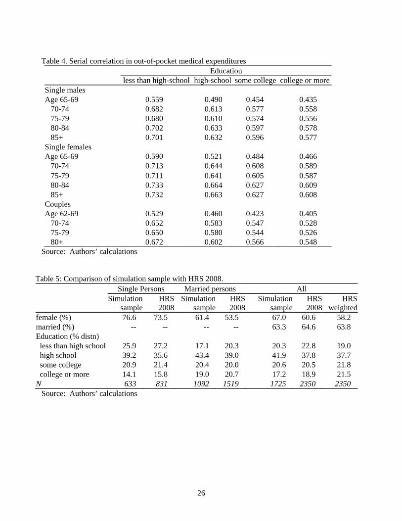
26

Table 4. Serial correlation in out-of-pocket medical expenditures Education less than high-school high-school some college college or moreSingle males Age 65-69 0.559 0.490 0.454 0.435

70-74 0.682 0.613 0.577 0.558 75-79 0.680 0.610 0.574 0.556 80-84 0.702 0.633 0.597 0.578 85+ 0.701 0.632 0.596 0.577

Single females Age 65-69 0.590 0.521 0.484 0.466

70-74 0.713 0.644 0.608 0.589 75-79 0.711 0.641 0.605 0.587 80-84 0.733 0.664 0.627 0.609 85+ 0.732 0.663 0.627 0.608

Couples Age 62-69 0.529 0.460 0.423 0.405

70-74 0.652 0.583 0.547 0.528 75-79 0.650 0.580 0.544 0.526 80+ 0.672 0.602 0.566 0.548

Source: Authors’ calculations

Table 5: Comparison of simulation sample with HRS 2008. Single Persons Married persons All

Simulation

sample HRS 2008

Simulationsample

HRS 2008

Simulation sample

HRS 2008

HRS weighted

female (%) 76.6 73.5 61.4 53.5 67.0 60.6 58.2 married (%) -- -- -- -- 63.3 64.6 63.8 Education (% distn) less than high school 25.9 27.2 17.1 20.3 20.3 22.8 19.0 high school 39.2 35.6 43.4 39.0 41.9 37.8 37.7 some college 20.9 21.4 20.4 20.0 20.6 20.5 21.8 college or more 14.1 15.8 19.0 20.7 17.2 18.9 21.5 N 633 831 1092 1519 1725 2350 2350

Source: Authors’ calculations

27

Table 6. Economic resources and expenditures. Single persons, thousands 2008$

N percent positive

mean initial wealth

mean PV of

earnings

mean PV annuities

mean PV

taxes

mean PV consumption

mean excess wealth

median excess wealth

Less than high-school 164 45.6% 60.2 6.0 106.8 3.2 201.3 -30.9 -7.7 High-school 248 68.0% 232.2 13.8 193.0 23.3 266.8 149.5 74.4 Some college 132 66.6% 317.5 20.1 226.1 41.4 353.3 170.8 96.7 College and above 89 75.8% 538.2 44.0 329.2 95.3 490.9 325.1 201.3

All 633 63.0% 248.4 17.4 196.7 32.0 299.4 131.9 50.6 Source: Authors’ calculations Table 7. Economic resources and expenditures. Couples, thousands 2008$

N percent positive

mean initial wealth

mean PV of future

earnings

mean PV annuities

mean PV taxes

mean PV consumption

mean excess wealth

median excess wealth

Less than high-school 187 75.1 284.6 14.0 265.4 27.9 321.2 215.0 137.2 High-school 474 84.3 499.2 16.5 395.7 75.7 441.9 394.2 261.5 Some college 223 85.3 1,024.5 22.7 477.6 227.9 595.9 701.4 337.9 College and above 208 88.9 1,406.7 56.7 651.0 319.2 880.4 913.9 572.3

All 1,092 83.8 742.6 25.0 438.7 145.0 536.2 525.2 287.6 Source: Authors’ calculations

28

Table 8. Percent adequately prepared: 95 to 100 percent chance of dying with positive wealth

Single Persons Married Persons

All Males Females All Males Females

Less than high-school 33.5 60.6 26.7 66.8 65.5 68.0 High-school 54.4 61.9 51.9 77.4 74.7 78.8 Some college 50.8 62.5 47.0 76.2 73.4 77.8 College and above 61.8 65.0 60.9 85.1 83.3 86.6

All 49.3 62.2 45.4 76.8 74.6 78.2 Source: Authors’ calculations Table 9. Percent adequately prepared: 95 to 100 percent chance of dying with positive wealth after reducing consumption by 10%

Single Persons Married Persons

All Males Females All Males Females

Less than high-school 36.0 63.6 29.0 70.1 70.2 69.9 High-school 62.1 66.7 60.5 79.5 77.2 80.8 Some college 53.8 62.5 51.0 80.7 77.2 82.6 College and above 68.5 65.0 69.6 88.5 86.5 90.2

All 54.5 64.9 51.3 79.9 77.9 81.1 Source: Authors’ calculations

29

Table 10. Sensitivity of adequacy assessment to thresholds. Percent of persons adequately prepared based on variation in chances of dying with positive

wealth and reduction in initial consumption. Reduction in initial consumption

Percent chances of dying with positive wealth

Singles Married persons

5 percent 10 percent 15 percent 5 percent 10 percent 15 percent 95 51.8 54.5 57.2 78.3 79.9 81.4 90 55.3 58.0 61.1 79.8 81.2 83.0 85 57.8 60.8 63.5 80.7 82.3 84.6 80 59.7 62.1 64.9 81.5 83.0 86.1 Source: Authors’ calculations Table 11. Percent with adequate resources by financial planning horizon

Percent adequately prepared: 95 to 100 percent chance of dying with positive wealth after reducing consumption by 10% by financial planning horizon

Single Persons Married Persons

All Males Females All Males Females

Next few months 37.1 32.4 38.6 70.0 68.9 70.7 Next year 46.7 58.3 42.4 82.2 83.0 81.7 Next few years 67.7 81.1 63.7 78.7 79.0 78.6 Next 5 to 10 years 63.1 82.8 58.3 81.6 76.9 84.9

Longer than 10 years 60.0 80.0 53.3 86.2 84.3 87.5

Total 55.2 64.9 51.3 79.7 77.9 81.1 Source: Authors’ calculations

Table 12. Percent with adequate resources by self-rated health

Percent adequately prepared: 95 to 100 percent chance of dying with positive wealth after reducing consumption by 10% by self-rated health

Single Persons Married Persons

All Males Females All Males Females

Fair or poor 37.7 44.1 35.2 68.9 68.1 69.5

Good to excellent 62.5 78.7 58.2 83.3 81.5 84.4

Total 54.5 64.9 51.3 79.9 77.9 81.1 Source: Authors’ calculations

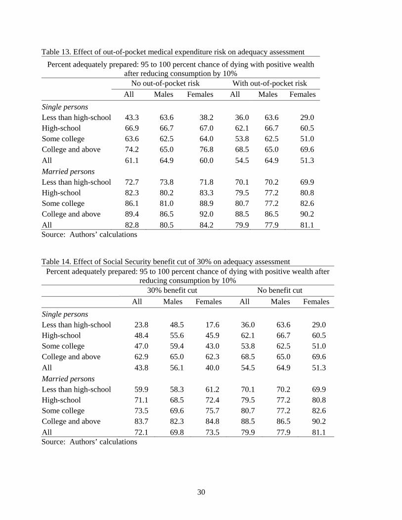
30

Table 13. Effect of out-of-pocket medical expenditure risk on adequacy assessment

Percent adequately prepared: 95 to 100 percent chance of dying with positive wealth after reducing consumption by 10%

No out-of-pocket risk With out-of-pocket risk

All Males Females All Males Females

Single persons Less than high-school 43.3 63.6 38.2 36.0 63.6 29.0 High-school 66.9 66.7 67.0 62.1 66.7 60.5 Some college 63.6 62.5 64.0 53.8 62.5 51.0 College and above 74.2 65.0 76.8 68.5 65.0 69.6

All 61.1 64.9 60.0 54.5 64.9 51.3

Married persons Less than high-school 72.7 73.8 71.8 70.1 70.2 69.9 High-school 82.3 80.2 83.3 79.5 77.2 80.8 Some college 86.1 81.0 88.9 80.7 77.2 82.6 College and above 89.4 86.5 92.0 88.5 86.5 90.2

All 82.8 80.5 84.2 79.9 77.9 81.1 Source: Authors’ calculations Table 14. Effect of Social Security benefit cut of 30% on adequacy assessment

Percent adequately prepared: 95 to 100 percent chance of dying with positive wealth after reducing consumption by 10%

30% benefit cut No benefit cut

All Males Females All Males Females

Single persons Less than high-school 23.8 48.5 17.6 36.0 63.6 29.0 High-school 48.4 55.6 45.9 62.1 66.7 60.5 Some college 47.0 59.4 43.0 53.8 62.5 51.0 College and above 62.9 65.0 62.3 68.5 65.0 69.6

All 43.8 56.1 40.0 54.5 64.9 51.3

Married persons Less than high-school 59.9 58.3 61.2 70.1 70.2 69.9 High-school 71.1 68.5 72.4 79.5 77.2 80.8 Some college 73.5 69.6 75.7 80.7 77.2 82.6 College and above 83.7 82.3 84.8 88.5 86.5 90.2

All 72.1 69.8 73.5 79.9 77.9 81.1 Source: Authors’ calculations

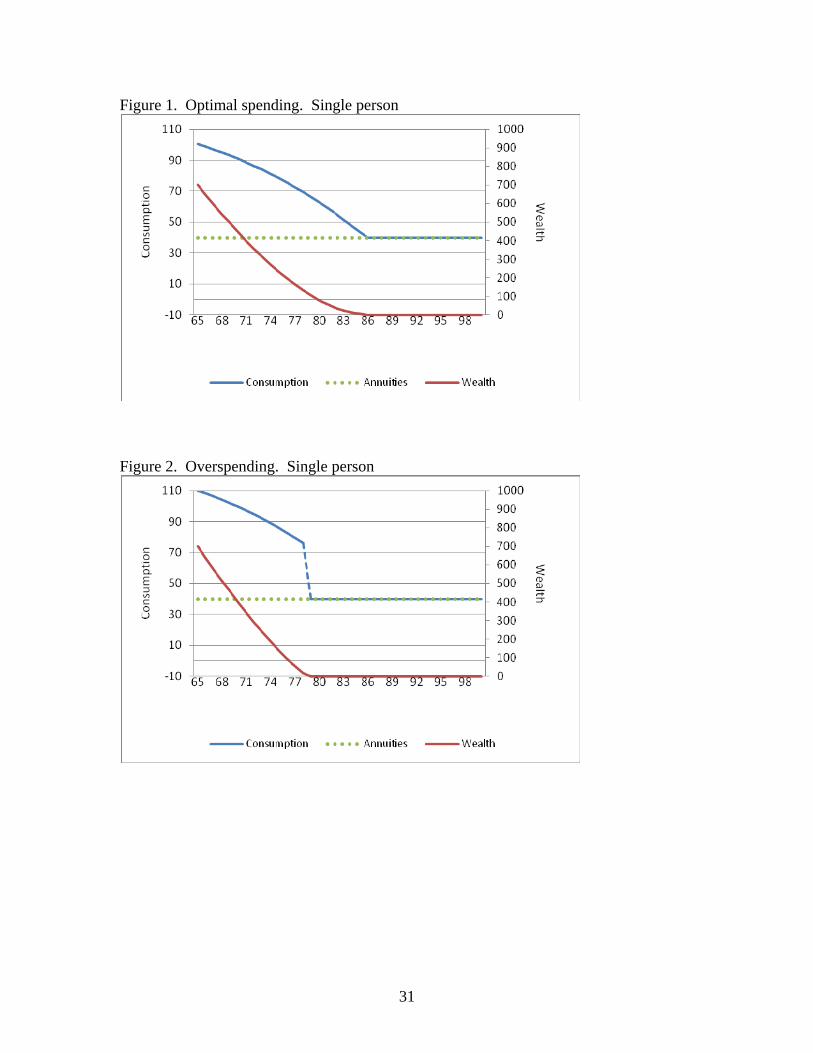
31

Figure 1. Optimal spending. Single person

Figure 2. Overspending. Single person

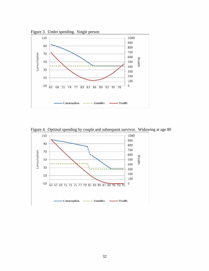
32

Figure 3. Under spending. Single person

Figure 4. Optimal spending by couple and subsequent survivor. Widowing at age 80

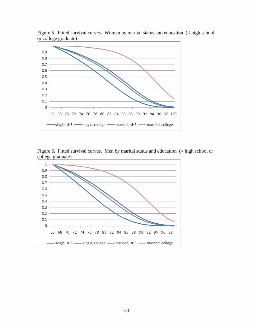
33

Figure 5. Fitted survival curves. Women by marital status and education (< high school or college graduate)

Figure 6. Fitted survival curves. Men by marital status and education (< high school or college graduate)

34

Figure 7. Fitted life-cycle consumption paths. Single females

0

20

40

60

80

100

120

65 67 69 71 73 75 77 79 81 83 85 87 89 91 93 95

<high school

high school

some college

college grad

model

Figure 8. Fitted life-cycle consumption paths. Married persons. Age is husband’s age. Age difference between husband and wife five years or less