ECONOMIC DEVELOPMENTAND EMISSION CONTROL OVER THE …

ECONOMIC DEVELOPMENT AND EMISSION CONTROL OVER THELONG TERM: THE ICLIPS AGGREGATED ECONOMIC MODEL

MARIAN LEIMBACH and FERENC L. TOTHPotsdam Institute for Climate Impact Research, Postfach 601203, D-14412 Potsdam, Germany

Abstract. In integrated assessments of climate change, greenhouse-gas emissions and climate changeimpacts provide the linkages between the world economy and the climate system. Key climaticprocesses operate at the scales of centuries. This requires highly aggregated models for portrayingthe dynamics of the economic system. An extended Ramsey-type optimal growth model is presentedas the appropriate tool to be integrated with a reduced-form climate model in the ICLIPS integratedassessment. The eleven-region model of the world economy involves exogenous population and en-dogenous investment dynamics with productivity progress based on a technological diffusion model.World regions are linked via intertemporal trade flows of the composite consumption/investmentgood, capital mobility, and emission permit trading. Coupled with the ICLIPS Climate Model, theAggregated Economic Model can determine corridors of permitted long-term carbon emission pathsor, as primarily discussed in this paper, specific cost-effective emission trajectories. The sensitivityof mitigation costs to externally specified climate change/impact constraints and to to assumptionsabout non-CO� greenhouse-gas emissions flexibility is also discussed.

Keywords: climate stabilization target, integrated assessment, long-term economic model, tolerablewindows approach

Abbreviations: AEM – Aggregated Economic Model; IAM – integrated assessment model; ICLIPS– Integrated Assessment of Climate Protection Strategies; GHG – greenhouse gas

1. Overview and Objectives

One of the main challenges faced by developers of Integrated Assessment Models(IAMs) addressing the climate change problem is to find the proper compromisebetween the spatial and temporal scales and resolutions of the models they need tointegrate. The nature of climatic change (global, long-term problem with diversesources and a multitude of impacts) requires a global model with some regionaldetail that covers dynamic processes of socioeconomic development and environ-mental change over at least a century. This leaves little choice for economistsin selecting their tools: highly aggregated and drastically simplified models areneeded to capture the key factors and processes that determine future emissionsof greenhouse-gases (GHGs) and the social costs of their control. The DICE/RICEfamily of models (see Nordhaus, 1992, 1994; Nordhaus and Boyer, 2000), MERGE(Manne et al. 1995) or MiniCAM (Edmonds et al., 1996) demonstrate differentways to tackle this problem.

As explained and illustrated in earlier papers in this Special Issue, the mandatefor the project on Integrated Assessment of Climate Protection Strategies (ICLIPS)is to develop an IAM suitable to conduct inverse assessments of long-term climate

Climatic Change 00: 1–27, 2002.c� 2002 Kluwer Academic Publishers. Printed in the Netherlands.

econmod-0327.tex; 27/03/2002; 16:37; p.1

2 M. LEIMBACH AND F.L. TOTH

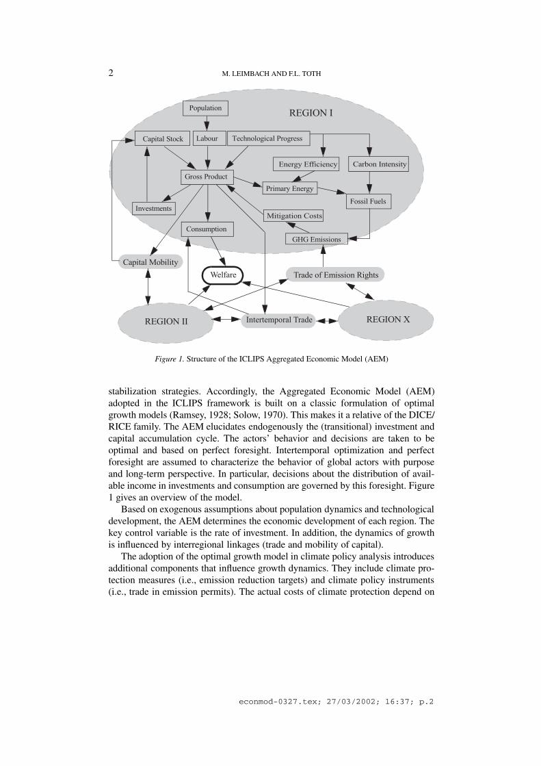
Figure 1. Structure of the ICLIPS Aggregated Economic Model (AEM)

stabilization strategies. Accordingly, the Aggregated Economic Model (AEM)adopted in the ICLIPS framework is built on a classic formulation of optimalgrowth models (Ramsey, 1928; Solow, 1970). This makes it a relative of the DICE/RICE family. The AEM elucidates endogenously the (transitional) investment andcapital accumulation cycle. The actors’ behavior and decisions are taken to beoptimal and based on perfect foresight. Intertemporal optimization and perfectforesight are assumed to characterize the behavior of global actors with purposeand long-term perspective. In particular, decisions about the distribution of avail-able income in investments and consumption are governed by this foresight. Figure1 gives an overview of the model.

Based on exogenous assumptions about population dynamics and technologicaldevelopment, the AEM determines the economic development of each region. Thekey control variable is the rate of investment. In addition, the dynamics of growthis influenced by interregional linkages (trade and mobility of capital).

The adoption of the optimal growth model in climate policy analysis introducesadditional components that influence growth dynamics. They include climate pro-tection measures (i.e., emission reduction targets) and climate policy instruments(i.e., trade in emission permits). The actual costs of climate protection depend on

econmod-0327.tex; 27/03/2002; 16:37; p.2

THE ICLIPS AGGREGATED ECONOMIC MODEL 3

the user-defined scheme of burden sharing and on the regional dynamic mitigationcost functions.

Similarly to all other IAMs, the ICLIPS AEM takes on the risky business oflooking into the distant future. However, it is by no means a forecasting model.It is driven by a large number of assumptions included in model parameters orexogenous scenario variables. Nevertheless, the model provides consistent imagesof the future and useful insights for climate policy.

2. The Structure of the Aggregated Economic Model

This section presents an overview of the AEM structure and explains the modelequations in a succinct form. Throughout this presentation, we use the followingindices:

i, h - regions

j - greenhouse gases

k - traded goods (1 = composite good; 2 = emission permits)

t, � - time index

r - iteration index.Social welfare represents the target criterion in setting and assessing the path of

optimal growth. The economic growth model assumes utility-maximizing actorsand includes a welfare optimizing “Global Planner”. Welfare (W) is measured asthe utility of per capita consumption (c):

� � ��

� �� (1)

The logarithmic utility function implies that an incremental unit of income inregions and for generations with low income produces a greater contribution totheir welfare than for their more affluent counterparts. The discount factor, thatincludes the pure rate of time preference �, determines the extent to which currentconsumption is traded off against future consumption. POP is the population sizeand nw is a weighting factor in aggregating regional welfare values in a globalwelfare function (see Section 3 and Appendix).

The main component of the growth model is the macroeconomic productionfunction. It represents the physical volume of production (measured in US$) as afunction of the physical volume of production factors, capital and labor (capitalis also measured in monetary units adjusted to price influences). The productionfunction thus reflects the technological characteristics of aggregated productionprocesses.

In the ICLIPS AEM, a Cobb-Douglas function is used. It assumes a constantelasticity of substitution of production factors and constant returns to scale, i.e., +�=1:

��

�� (2)

econmod-0327.tex; 27/03/2002; 16:37; p.3


Y is the output, K is capital POP represents labor, is the output-capital elas-ticity, � the output-labor elasticity and A represents total factor productivity (TFP).Although this suggests that theoretically the production factors capital and laborcan be substituted indefinitely, these processes do have economic limits as a resultof declining marginal productivities.

The objective of the AEM is to describe the processes of economic developmentover time (e.g., gross national product, per capita income) rather than their constantor steady state growth rates. This approach is based on the combination of theendogenous capital accumulation cycle and a technological diffusion model (cf.Ciscar and Soria, 2000).

The capital accumulation cycle (with investments I and depreciation rate Æ) isbased on investment decisions that, for any point in time, compare current reductionof consumption to a later increase of consumption resulting from expansion of thebasis of production:

�� Æ�� (3)

Technological progress is represented by a simple diffusion equation, presup-posing the convergence of total factor productivity change rates (tfpr) under theassumption that production technologies will be exchanged between developedand less developed regions. A diffusion parameter (tdf) determines the speed ofthis adjustment:

�� (4)

�� (5)

where tfpr�� is the exogenously specified growth rate of TFP in the most ad-vanced region.

The AEM is a multiregional global model. Although this makes data collectionand scenario specification considerably more difficult, it provides a better descrip-tion of the dynamics relevant to climate change. The model can cope with thedisparate present conditions and future development paths of different regions. Itcan also depict essential elements of growth dynamics that result from interactionsamong regions. Finally, regional differences in mitigation potentials and conflictinginterests in climate policy can also be studied.

Three fundamental types of interregional relations are distinguished in ourAEM: intertemporal trade, mobility of capital, and trade in emission rights.

Taking the form of direct foreign investments, the mobility of capital is a fun-damental element of the growth dynamics. International capital transfers are moti-vated by differences in regional rates of return to capital. This accelerates economicdevelopment in the capital importing regions while the source regions also benefitfrom higher returns. Transfers of capital (CA) between regions are balanced in eachperiod:

�� (6)

econmod-0327.tex; 27/03/2002; 16:37; p.4


Trade in capital, unlike other forms of trade, generates net foreign assets (NFA)and establishes a claim for interest (RR) by the exporter:

�� (7)

with�� Æ�� (8)

It is difficult for economic theory to explain why, in spite of higher return ratesin developing regions, the flow of capital to these regions is relatively small. Theusual explanation is that investors in developing regions have to pay an implied riskpremium. Recent attempts to explain this phenomenon start from a non-equilibriummodel that takes errors in estimating return rates into account in explaining in-ternational mobility of capital (Ianchovichina et al., 1999). In our model, capitalmobility is approximately adjusted to real trade flows by keeping interest rates onlyat the level of internationally averaged return rates on capital and simultaneouslylimiting the volume of capital flows and net foreign assets to a certain percentageof total gross product (fmax, fmin, expo, impo). This yields:

�� !"# � �� (9a)

�� !�� (9b)

Terminal conditions of the model prescribe that all foreign assets are withdrawnand thus all obligations from capital transfers are fulfilled by the end of the timehorizon:

�� (10)

The following current account restrictions affect both capital mobility and tradeflows (NTX):

�� $�� #� � �� % � �� (11a)

�� $�� !� � �� % � �� (11b)

In the model setting described in Section 5.2 (policy scenario 1), there is a jointbinding rate of around 50% for the constraints (9) and 70% for the constraints(11), with constraint (11b) as most restrictive in quantity (nearly 50%) as well asin quality (highest marginal values).

In a sectorally aggregated model producing one homogenous composite good,commodity trade takes place only if temporal flexibility (temporary trade deficit) ispermitted and when paying for emission permits. Exports and imports of emissionpermits and the composite good are balanced in each period:

��$�� % � �� (12)

Each region exports to and imports from a common pool. This formulationyields transparency and numerical efficiency.

econmod-0327.tex; 27/03/2002; 16:37; p.5


Emissions trading is an essential feature of the model. The exchange of “physi-cal” units of emission rights (measured for instance in gigatons (Gt) of carbon) hasto be distinguished from the payment for it (in units of the composite good). Theseexchange processes do not necessarily occur in the same period.

Emission trading in AEM is based on the concept of differentiated burdensharing (as agreed in the Kyoto Protocol). This is implemented through the initialallocation of emission rights rather than by setting regional reduction targets. Theregions’ share in the pool of total emission rights is specified while the absolutelevel of allocated emission rights is determined endogenously.� Based on the ini-tial allocation of emission rights and unlimited permit trading, emissions can bereduced in regions with the lowest marginal abatement costs. This arrangementmaximizes emissions reductions for a given cost or minimizes the costs for a givenreduction target.

The initial distribution of emission rights exerts a decisive influence on the priceof the emission rights and on the extent of permit trade. The criteria to use indistributing emission rights are fiercely debated on economic, political, and ethicalgrounds (see, e.g., Rose et al, 1998; Ringius et al., 1998). Many analysts argue thatin the long term an equal per capita distribution seems to be the fairest solution. Inthe short term, however, this distribution principle would give developing countriesa great advantage (they could sell a large part of their emission rights). In the worldof political reality, there is little chance of such a burden-sharing scheme beingaccepted in the near future.

A combined distribution principle has perhaps a greater chance of actually beingimplemented. We assume an allocation routine in which an initial grandfathering(status quo) distribution of emission rights gradually turns into a per capita distri-bution (whereby it must be noted that such a distribution is relatively unfavorable torapidly expanding regions such as China and Southeast Asia). With SH and PSH asone region’s shares in the pool of global emission rights and in global population,respectively, and with LQ as the period during which the transition to equal percapita distribution is completed, we get:

&'�� &'�� ()� � � � � � (13)

&'�� ()� �� &'�� &'�� ()� ��

� � �� ()� �� (14)

Another important choice to be made is whether to use a static or a dynamically-adjusted basis in the per capita distribution. The former allocates emission rightsaccording to the population distribution in a particular year while the latter observes

� The intended long-term analysis goes far beyond the time horizon of the Kyoto Protocol. Short-term adaptation and mitigation measures are not considered in detail. Hence, we do not attempt tobase the analysis on the specific reduction targets of the Kyoto Protocol.

econmod-0327.tex; 27/03/2002; 16:37; p.6


changes in population distribution. The former option could provide a stimulus toan active demographic policy.

A further point in climate policy discussions concerns the limitation of tradein emission rights. This would increase mitigation costs in general. The intentionis to limit the trade in so-called “hot air” or “tropical air” (emission rights thatcannot be utilized economically) and to induce technological change by obligingthe industrial nations to undertake emission reduction efforts domestically. Theexport of emission rights can be restricted most efficiently in relation to the amountof originally allocated emission rights. If xperm represents the respective shareparameter, and GLR is the global pool of emission rights, we get:

��$�� #��! � &'�� *(�� % � � � � �� (15)

Restrictions on emission rights import are related to actual emissions (with mpermas cap):

��$�� !��! � +,��

� � �� - � ‘CO2’� % � � � � �� (16)

When emissions reductions are required, and restrictions (15) and (16) hold,regions would buy emission permits as long as the purchase price is lower thantheir marginal abatement costs. Similarly, other regions sell their emission permitswhile their mitigation costs remain below the permit price. By assuming unlimitedtrading and no transaction costs, marginal costs of abatement will be equalizedglobally.

The regional costs of emission reductions are represented by dynamic miti-gation cost functions. In integrated assessment models, mitigation cost functionsrepresent the link between the magnitude of emission reductions relative to a ref-erence path and the resulting economic costs. Traditional mitigation cost functionsare quasi-static functions that are actually valid only for a single point in time.The parameters in traditional mitigation cost functions (see Nordhaus, 1994) areconstant (at least for long periods), i.e., the cost of subsequent emission reduc-tions is the same regardless of preceding reduction efforts. Research by Grublerand Messner (1998) explore explicit mitigation cost functions that alleviate theseshortcomings by considering cumulative (learning) processes. In addition to thecustomary progressive cost dynamics (cost parameter b2>1 in Equation (19) be-low), technological learning leads to relative cost reductions, i.e., the larger thevolume of reduction already undertaken, the cheaper further reduction becomes.This relationship is implemented in AEM by linking the mitigation costs to thecumulative amount of reduction.

The mitigation cost function implemented in our model hides basic relation-ships of the energy system (see Section 4). It consists of four equations and appliesto CO� only. Climate protection measures absorb a part of the produced grossproduct which is then no longer available for investments or for private and pub-lic consumption. The income loss, expressed in terms of gross domestic product

econmod-0327.tex; 27/03/2002; 16:37; p.7


(GDP) loss, in any given period is the difference in potential cumulative loss ofregional gross product (GPLO) between two consecutive periods of time (see alsoGritsevskii and Schrattenholzer, 2002):

�� *�(�� *�(�� (17)

where NY represents the gross product net of climate protection cost.The potential cumulative loss in GDP in year t is given by the sum of gross

product calculated for the years 1 to t, weighted by the mitigation costs (DCR) forthe year t:

*�(�� .�� - � ‘CO2’� � � �� (18)

The equation for determining DCR formally corresponds to a traditional mit-igation cost function, with enhanced regional and temporal resolution. However,the independent variable is not the emission reduction (related to the referenceemission path BEM) in year t, but the cumulative amount of emission reduction /:

.�� 0�� /�� - � ‘CO2’� � � �� (19)

where

/�� 1+,�� +,�� 1+,��

� � �� - � ‘CO2’� � � �� (20)

EM represents the actual emissions, and BEM is the reference emission. The costfunction parameters 0� and 0 are time-dependent and regionally differentiated.Reference emissions are computed ex ante as the product of carbon intensity, en-ergy intensity, and total output in a restricted model setting containing equations(1)-(12), (24) and (25).

The emission variable EM is derived from the equations of the mitigation costfunction. Due to a climate protection objective (or an impact threshold), emissionsare expected to diverge from the baseline (reference path). Two equations describeadditional constraints. The first one requires emissions not to exceed the amount ofallocated plus imported emission permits:

+,�� &'�� *(�� $��

� � �� - � ‘CO2’� % � � � � �� (21)

The second constraint keeps the sum of regional emissions below the global emis-sion limit:

��+,�� *(�� - � ‘CO2’� � � �� (22)

Due to the effect of discounting, the weight of incomes in the more distant futureis declining in the present-value welfare measure. Simultaneously, mitigation costs

econmod-0327.tex; 27/03/2002; 16:37; p.8


significantly decrease over time due to autonomous efficiency improvements (i.e.0�� 2 0��). The latter may dominate the cost-reducing effect of learning-by-doing and could imply drastic reductions in later periods at nearly no costs evenwithout earlier mitigation. In order to restrict extreme model behavior, the emissionreduction rate is limited to err:

��+,�� +,�� - � �� !� � � �� (23)

The income computed in Equation (17) is reduced by net exports and increasedby net imports (negative CA and NTX). We close our model with the followingbalance equation that determines the consumption level C:

�� $�� % � �� (24)

Per capita consumption is derived by:

�� (25)

Finally, at the interface between the climate and the economy model, the fol-lowing equation determines the trajectory of total emissions (E):

+�� +,�� (3+,�� - � �� !� � � �� (26)

where LUEM accounts for emissions from land-use change, either exogenouslyspecified or provided by the ICLIPS land-use change module.

SO� emissions are strongly correlated with industrial CO� emissions, but alsosubject to an autonomous desulfurization process by rate sulfred:

+,�� +,�� +,�� +,�� 45��

� � �� - � ‘SO2’� � � �� (27)

3. Intertemporal Equilibrium Solution

Economic growth models belong to the group of optimization models whose solu-tion algorithms presuppose the formulation of a single target criterion (which maywell be synthetic). A Pareto-optimal solution is normally obtained by choosinga global (weighted) objective function embracing welfare gains in all regions. Inmodels with multiple actors, however, development options of the individual actorsand their trading strategies cannot be determined independently from one another.

The AEM assumes that states co-operate in trading and climate policy, but fol-low national interests in income distribution. One implication is that all regionshave to eliminate their accumulated trade deficits in the long term. All interre-gional trade flows and transfers have to be balanced to simultaneously satisfy

econmod-0327.tex; 27/03/2002; 16:37; p.9


national/regional budget constraints. This budget balancing is a non-trivial problembecause essential price information (e.g., the price of emission permits) are a prioriunknown on the one hand, and import and export take place at different times(and thus at different prices), on the other. Omitting these trade balance deficitswould contradict real economic processes and ignore an essential element of futureeconomic dynamics.

Two approaches are implemented in the AEM to resolve this problem. The firstone applies the method of sequential joint maximization (Dixon, 1975; Manneand Rutherford, 1994). It consists of adapting welfare weights that measure theregional contributions to the global objective function in such a way that budgetconstraints are always satisfied in the equilibrium solution. The existence of suchan equilibrium solution has been proven by Negishi (1972). The adjustment of thewelfare weights (also called Negishi weights) on the basis of intertemporal tradebalance deficits takes place iteratively between two complete optimization runs.The technical details of this procedure are described in the Appendix.

The second approach is used in our model to deal with interregional interactionsrelated to capital mobility. The stock of foreign assets is updated on the basisof capital flows. The interest accruing to this amount is immediately calculatedaccording to the globally averaged rate of return to capital. When the terminalcondition (all foreign assets will be removed in the final period) is included, theabove procedure of eliminating trade deficits causes all budget constraints to befulfilled.

4. Data Base and Empirical Foundations

The AEM can be run in two modes: reference mode and policy mode. In referencemode, several equations are suppressed (e.g., mitigation cost functions, distributionof and trade in emission rights) and the economic model is allowed to determine theoptimal development paths based on different scenarios of main exogenous drivingforces (population dynamics, technological change) and parameters (e.g., diffusionparameter, depreciation rates, discount rates). In order to simplify the subsequentdiscussion (in terms of input data and results), we present one reference scenariothat also serves as the basis for the policy scenarios. In order to ensure consistencyacross different model components, some parameter in AEM are predetermined bythe scenario underlying the mitigation cost function. This is essential due to thefact that by means of the mitigation cost functions the AEM integrates insights ofthe energy sector which are needed in order to get some reasonable estimates ofthe costs of emission reduction (see below). The model distinguishes 11 regions:

econmod-0327.tex; 27/03/2002; 16:37; p.10


AFR - Sub-Saharan Africa

CPA - China, Mongolia, Vietnam, Cambodia, Laos

EEU - Eastern Europe

FSU - Former Soviet Union

LAM - Latin America and the Caribbean

MEA - Middle East and North Africa

NAM - North America

PAO - Pacific OECD (Japan, Australia, New Zealand)

PAS - Other Pacific Asia

SAS - South Asia (mainly India)

WEU - Western Europe.A large part of the input data for the model (population, carbon intensities, en-

ergy efficiency improvements, initial values for gross domestic product and capitalstock) is based on the IIASA Reference Scenario F (Gritsevskii and Schratten-holzer, 2002). This scenario is similar to the A2 scenario of the World EnergyCouncil (see Nakicenovic, 1998) and resembles the IPCC SRES A2 scenario (Na-kicenovic et al., 2000). Reference Scenario F largely extrapolates current eco-nomic, technological and environmental trends. It is a growth-oriented, emission-intensive scenario that forms a suitable basis of comparison for the analysis ofalternative policy scenarios. It assumes a population of 10.1 billion in the year2050. High rates of economic growth lead to a five-fold increase in the globalgross product by the year 2050 compared to 1990 and to an 18-fold increase bythe year 2100 (compared to a factor of 12 in the IPCC IS92a scenario). The tech-nological changes are moderate (roughly 1% annual reduction in energy intensityglobally) and the fossil resource pool is confined to those currently exploitable plusalready identified reserves. Coal continues to play a dominant role in providingenergy throughout the next century. The proportion of the non-fossil energy sourcesincreases to around 50% by 2100.

The Reference Scenario F imposes a significant impact on the environment.In addition to climate change, these environmental impacts include effects asso-ciated with increased SO� emissions: health impacts, acidification of soils andlakes, forests damage, etc. It is not assumed that future societies will toleratesuch impacts. Nevertheless, this scenario presents a useful reference case for ouranalyses.

The model’s empirical foundation includes the parameter estimation and cali-bration of the Cobb-Douglas production function, the regional depreciation ratesof the capital stock, and the mitigation cost function. Parameters for the latterare derived from a statistical evaluation of many computed scenarios using thecoupled MACRO-MESSAGE model and the IIASA scenario database (Gritsevskiiand Schrattenholzer, 2002; Schrattenholzer and Schafer, 1996). As a result, eachsingle parameter of the mitigation cost function aggregates interdependencies from

econmod-0327.tex; 27/03/2002; 16:37; p.11


resource extraction to the provision of energy end-use services. The parametersintegrate the utilization of domestic resources, energy imports/exports and relatedmonetary flows, investment requirements, the types of production or conversiontechnologies selected as well as interfuel and energy-capital substitution processes.Hence, each unit of carbon emission reduction in the model is linked to specificchanges in the energy system.

The Cobb-Douglas production function requires the calibration of two param-eters: the total factor productivity (TFP) and the elasticity parameter . We havetaken elasticity values adopted in similar models, specifically the values used inthe MERGE model (Manne et al., 1995) for the base year 1990. From then on,however, temporal variation is assumed in the regionally differentiated parameters.By 2050, the TFP parameters for all regions converge at around 0.25.

The development of TFP is predetermined in a phase of calculations precedingthe actual model calculations and is thus exogenous. The rates of change in TFP aredetermined on the basis of a technological diffusion model. This model assumesthat, through the transfer of technology and knowledge, in the long term all re-gions reach a level of productivity equal to that of the most advanced regions. Thisdiffusion and convergence process, however, occurs at different rates in differentregions. Thus, EEU or FSU have higher diffusion rates than, e.g., AFR or MEA.The concrete parameter values are in turn adjusted so that the resulting economicdevelopment in the reference run depicts the development of the IIASA referencescenario F.

The starting point for the calculation of the physical capital stock is derived fromdata on investments from national accounting (World Bank, 1999). For many coun-tries, additional sufficiently long time series (divided into five categories: machinesand equipments, means of transport, business premises, dwellings, other buildings)are provided by the Penn World Tables 5.6a (see Summers and Heston, 1991). Alinear model with two predictors (material welfare, expressed as a logarithm ofthe per capita gross national product, and time as the year of investment) is fittedto these data in order to estimate investments in the individual categories also forcountries for which only aggregated data on investments are available. By using thedifferentiated depreciation rates from the Penn World Tables, the net capital stockin each of these categories is finally calculated as the residual value of cumulativeinvestments at constant replacement prices on the basis of degressive (geometric)depreciation. The evolution of aggregated depreciation rates is derived from thehistoric time series of capital stock determined this way. For the long-term scenariohorizon, however, it appears to be more realistic to assume convergence rather thana long-lasting continuation of past trends. Under the hypothesis that, particularlyin developing countries, short-lived categories of investment goods (e.g., machinesand means of transport) are increasingly used, we assume a long-term stabilizationof the depreciation rates at 9%.

econmod-0327.tex; 27/03/2002; 16:37; p.12


5. Model Application for Cost-effectiveness Analysis

The main application of the ICLIPS IAM is to explore corridors of long-term car-bon emissions under user-specified levels of acceptable climate change impacts andmitigation costs. Such applications are presented in the twin papers on integratedassessment of long-term climate policies in this Special Issue (Toth et al., 2002a,2002b). Here we present only one prominent path within the corridors - the cost-effective emission path. We present detailed results that complement the corridorresults associated with any user-specified targets. Our focus is on the mitigationcosts and on the question how the burden of emissions reduction may be sharedbetween the world regions in the long run. We explore cost sensitivities and com-pare our cost-effective paths and other results to those of similar models. First wepresent the reference run, then we turn to the results of the policy runs.

5.1. REFERENCE RUN

In the reference run, baseline welfare and emission paths are established by as-suming that no climate policy is needed. The path of uncontrolled emission ofGHGs implies reference welfare values that are merely hypothetical, because theydo not consider damages caused by the induced climate change. The differencesin welfare between control runs and the reference run, however, can be taken tocompare the social costs of different climate policy interventions to reach the sameclimate/impact target.

According to the results of the reference run, the regions can be assigned to oneof four groups with regard to long-term economic development:1. moderate growth on a high level: NAM, PAO, WEU;2. accelerated growth: EEU, FSU, PAS;3. medium growth: CPA, MEA, LAM;4. delayed growth: AFR, SAS.

Figure 2 shows the development of incomes in 5 of the 11 world regions mea-sured in constant 1985 US dollar (this unit also applies to monetary figures pre-sented graphically below). The differences in welfare between western industrialnations and other regions of the world increase initially. By the end of the 21�� cen-tury, the dynamics of development in the less developed regions begin to catch up atincreasing speed. This pattern of development is largely determined by exogenousassumptions and founded only to a small extent endogenously.

GHG emissions increase in almost all regions. Increases are drastic in CPA andSAS (Figure 3). Apart from LAM, PAO, and WEU, reductions in energy intensityand carbon intensity cannot compensate increasing emissions due to populationand economic growth. In addition, according to the underlying baseline scenario,the proportion of coal used in energy production increases again in the mid-21stcentury, causing the decline in carbon intensity to cease in many cases. This isshown clearly by the renewed rise of emissions in CPA after 2050, and as an

econmod-0327.tex; 27/03/2002; 16:37; p.13


0

20

40

60

80

100

1990

2000

2010

2020

2030

2040

2050

2060

2070

2080

2090

2100

Pe

rca

pita

co

nsu

mp

tio

n(U

SD

10

00

)

AFR

CPA

FSU

NAM

WEU

Figure 2. Economic development in the reference run

outcome of the economic upsurge in SAS, MEA, or AFR. The combined effectis an accelerated increase in global emissions up to around 25 GtC in the year2100.

0.0

1.0

2.0

3.0

4.0

5.0

6.0

1990

2000

2010

2020

2030

2040

2050

2060

2070

2080

2090

2100

Industr

ialC

O2

em

issio

ns

(GtC

)

CPA

FSU

NAM

SAS

WEU

Figure 3. Industrial CO� emissions in the reference run

econmod-0327.tex; 27/03/2002; 16:37; p.14


The rise in global CO� emission is accompanied by a proportional rise in theaerosol-forming SO� emissions (which therefore have a cooling effect). The as-sumption of a strong correlation between SO� and CO� is supported by the under-lying IIASA base scenario F and justified again by the increasing share of coal.The AEM assumes an autonomous desulfurization rate of 0.5% annually.

The climate change induced by this reference scenario is computed by couplingwith the ICLIPS Climate Model. This requires additional assumptions about theemissions of other greenhouse gases. Emissions of ozone-depleting gases are pre-scribed according to the Montreal Protocol and its amendments in all cases. Twoscenarios are distinguished for emissions of the other non-CO� greenhouse gases.In the first scenario, the values of 1990 are kept constant while in the second caseemissions of non-CO� GHGs follow the IPCC IS92a scenario. A temperature curvewith a slightly higher increase results from the increase in non-CO� emissions.For the year 2100, Scenario 1 calculates a temperature increase of around 1.8 ÆCrelative to pre-industrial values, by the year 2200 the increase is around 3.8 ÆC.(The climate sensitivity parameter anchored in the climate model at 2.5 ÆC underdoubled CO� equivalent GHG concentration represents the “best estimate” of theIntergovernmental Panel on Climate Change (IPCC, 1996)). As a result of theincrease in non-CO� emissions in Scenario 2, the correspondingly higher valuesin 2100 and 2200 are 2.1 and 4.2 ÆC, respectively.

5.2. POLICY RUNS FOR A CLIMATE WINDOW

5.2.1. Key assumptionsTaking the reference run described in the previous section as a starting point,policy scenarios in the framework of cost-effectiveness calculations are analyzedwith the ICLIPS Integrated Climate-Economy Model. A policy scenario is de-fined by the formulation of climate change/impact targets. In cost-effectivenessanalyses, we search for the least-cost emission path to reach a pre-determinedclimate change target while achieving the greatest possible welfare. The policy tar-get we explore stems from the German Environmental Council on Global Change(WBGU, 1995)(Figure 4).

The Council reviews the range of variability of the global mean temperature inthe late Quarternary, the geological period that shaped our present environment,and finds the minimum of 10.4 ÆC in the Wuerm ice age and the maximum of16.1 ÆC in the Eamian. The Council argues that a considerable departure fromthis range would imply major changes in the composition and function of to-day’s ecosystems but proposes to extend the range by 0.5 ÆC at both ends to arriveat a tolerable window for global mean temperature ranging from 9.9 to 16.6 ÆC.Moreover, based on arguments about adaptive capacity of various climate-sensitivesectors, the Council maintains that the rate of change in the global mean tempera-ture should not exceed 0.2 ÆC/decade. Taken together, these constraints define theWBGU climate window.

econmod-0327.tex; 27/03/2002; 16:37; p.15


Figure 4. The WBGU climate window

Although its origins go back to 1995, the Council’s proposal regarding thelong-term stabilization target remains influential in the policy debate, at least inGermany. It is one of the few normative targets published by a top-level advisoryboard to any government. The objective of our analysis is to demonstrate how theICLIPS IAM can explore the implications of normative targets proposed by thepolicy community. The analysis and results should not be interpreted as a science-based proposal by the authors or by the rest of the ICLIPS team. In fact, manyobservers maintain that, despite the geo-historical arguments, the WBGU target issomewhat arbitrary. It is important to note that the ICLIPS project encompassesClimate Impact Response Functions (Fussel et al., 2002) of various impact sectorsin order to help explore and make the choice of stabilization targets based onwhat are perceived to be unacceptable impacts of climate change. Incidentally,the WBGU climate window is similar in nature and magnitude to the long-termclimate change constraint (maximum 2 ÆC increase in global mean temperature)proposed by the European Union before the Kyoto Conference of the Parties tothe UNFCCC and comparable to the various sea-level rise limits suggested by theAlliance of Small Island States.

The analysis is based on the scenarios presented in the previous section. Theydiffer in their assumptions about non-CO� emissions as follows:� Scenario 1: constant CH� and N�O emissions� Scenario 2: CH� and N�O emissions according to IS92a (mostly increasing).

The policy scenarios consider emission permit trade among the Annex-I regionsfrom 2000 on. Non-Annex-I countries take part in international emission trade

econmod-0327.tex; 27/03/2002; 16:37; p.16


only from 2010 on. Similarly to capital transfer and intertemporal trade, the advalorem trade in emission permit is limited to 10% of the respective current grossregional product. Furthermore, there is no limitation on the physical amount ofemission rights that may be exported, while the share of reduction obligations thatmay be covered by emission permit imports is limited to 50%. Other importantassumptions in the model include a pure rate of time preference of 3% (same asin the reference run), and the completion of the transition to an equal per capitadistribution of emission rights by 2050 (based on 2025 population).

5.2.2. ResultsIn reviewing the results below, it is important to keep in mind that the two scenariosdeliver complementary information. To be exact, they represent a single policyscenario with differing underlying assumptions, with important implications forcomparing the mitigation costs of the two scenarios. These costs are significantlyhigher for Scenario 2 because of the higher baseline emissions of non-CO� GHGs.Correspondingly, the implicitly avoided damages are higher. A discussion of thetwo scenarios helps to clarify the dependence of mitigation costs on exogenousmodeling assumptions.

Figure 5 shows income losses (in %) relative to the reference scenario. Incomelosses are measured as per capita consumption losses. In Scenario 1, the lossesremain largely below 2%. Regions with losses above or near the 1% mark are CPA,EEU, FSU, NAM, and MEA, in other words regions with high per capita emissionsand/or with an economic sector strongly based on fossil energy resources. Thereare also regions (e.g., AFR, SAS) increasing per capita consumption relative to thereference scenario. It becomes much more expensive to satisfy the climate con-straint under Scenario 2. Some regions (CPA, FSU, PAS) fall below their referenceincome values by more than 5% . The enormous differences between Scenario1 and 2 are surprising as well as the interregional differences, which are alreadyvisible in Scenario 1, but become striking under Scenario 2. Figure 6 demonstratesthat there are also huge differences over time. While (according to Figure 6) inScenario 1 higher income losses are expected in the second half of the century,in Scenario 2 substantial losses already occur in the first half of the century. Thisapplies in particular to CPA and NAM. Gains in SAS and AFR as well as lossesin MEA and PAS arise similarly in the second half of the century. In order to findthe reasons for these results, we need to have a look at the associated “optimal”emission trajectories and trade flows of emission rights.

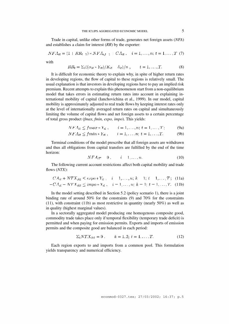
The “optimal” emission strategies determined by the model for selected regionsare presented in Figures 7 and 8. In Scenario 1, many developing regions canfollow their baseline emission paths for several decades, some of them well intothe second half of the 21st century. Industrial regions need to begin reducing emis-sions significantly much earlier. However, the transition phase (2000-2030) to forman energy-saving and less carbon-intensive economy is relatively long, mitigationcosts will therefore be moderate. Under Scenario 2, stricter CO� emission reduc-

econmod-0327.tex; 27/03/2002; 16:37; p.17


Scenario 1

-2.0

-1.0

0.0

1.0

2.0

3.0

4.0

5.0

6.0

7.0

AFR CPA FSU MEA NAM SAS WEU PAO PAS LAM EEUPe

rca

pita

co

nsu

mp

tio

nlo

ss

(%)

Scenario 2

-2.0

-1.0

0.0

1.0

2.0

3.0

4.0

5.0

6.0

7.0

AFR CPA FSU MEA NAM SAS WEU PAO PAS LAM EEUPe

rca

pita

co

nsu

mp

tio

nlo

ss

(%)

Figure 5. Average loss of per capita consumption between 1995 and 2100

tions are necessary, and costs increase. This additional control of CO� is required tocompensate the increasing radiative forcing caused by rising non-CO� emissions.These global reduction requirements are manifested in appreciably altered regionalemission paths relative to Scenario 1. In all Annex-I regions, emission reductionhas to begin much earlier and proceed considerably faster. Developing regions needto participate in emission reduction earlier. The case of China (region CPA) isparticularly interesting. China has to reduce its emissions drastically starting asearly as 2020. The local minimum in China’s emission curve in 2035 is a result ofthe climate window. The specified rate of temperature change constraint is likely tobecome binding soon. As major emitters, China and NAM need to undertake very

econmod-0327.tex; 27/03/2002; 16:37; p.18


-4.0

-3.0

-2.0

-1.0

0.0

1.0

2.0

3.0

4.0

1995-2015 2015-2040 2040-2070 2070-2100

Per

capita

consum

ption

loss

(%)

AFR

CPA

EEU

FSU

LAM

MEA

NAM

PAO

PAS

SAS

WEU

Figure 6. Average loss of per capita consumption in Scenario 1 for different periods

large reductions in order to keep the climate system within the specified globalclimate window.

While the climate window determines the overall emission reduction pattern,regional differences in the emission trajectories are heavily influenced by the allo-cation of emission rights. Although the transition period between the initial statusquo allocation and the final per capita allocation seems to be quite long, high percapita emitters (e.g., NAM) and fast developing regions (e.g., CPA, PAS, EEU) runquickly into shortage of emission rights. This shortage can either be resolved byenhanced domestic reduction efforts or massive imports of emission rights. Bothmight become costly.

The emission permit trade flows are presented in Figures 9 and 10. The generalstructure of the permit trade is robust. The main exporters are SAS, AFR, partlyLAM, and initially also FSU. The leading importers are CPA, NAM, and to a lesserextent MEA, PAS, and WEU. In Scenario 1, FSU changes from being an exporterin the first decades of the 21st century to an importer in later decades. In Scenario 1with virtually unlimited emission trade (the 50% import barrier has little restrictiveeffect), the extent of trade flows is very high. The volume of permit trade is lowerin Scenario 2, but it involves a considerably higher proportion of actual emissions.The fast increase in early decades is particularly striking.

Permit trade makes it possible to achieve climate protection targets on the onehand, and reduces the costs of emission reduction, on the other. The costs, mea-sured as changes in per capita income relative to the reference scenario, nonethelessvary widely. Regions like AFR and SAS can even exceed their reference income.This is made possible either by the sale of emission rights which cannot immedi-

econmod-0327.tex; 27/03/2002; 16:37; p.19


0.0

0.5

1.0

1.5

2.0

2.5

3.0

1990

2000

2010

2020

2030

2040

2050

2060

2070

2080

2090

2100

Industr

ialC

O2

em

issio

ns

(GtC

)

CPA

FSU

NAM

SAS

WEU

Figure 7. Industrial CO� emissions of selected regions in Scenario 1.

0.0

0.5

1.0

1.5

2.0

2.5

3.0

1990

2000

2010

2020

2030

2040

2050

2060

2070

2080

2090

2100

Industr

ialC

O2

em

issio

ns

(GtC

)

CPA

FSU

NAM

SAS

WEU

Figure 8. Industrial CO� emissions of selected regions in Scenario 2.

ately be used in an equally productive way, or by creating trade balance deficits(and thus increasing disposable domestic product) in expectation of later oppor-tunities to sell emission rights. In Scenario 2, exporters of emission rights canadditionally profit from the very high permit prices: 120$/tC on average, comparedto 15$/tC in Scenario 1. Among others, the differing permit prices explain thebig differences between Scenario 1 and 2 as well as between different regions.Emission rights exporting regions can use the income from trade to embark on a

econmod-0327.tex; 27/03/2002; 16:37; p.20


1990

2005

2020

2035

2050

2065

2080

2095

ME

A

WE

U

FS

U

AF

R

NA

M

CP

A

SA

S

-1.5

-1.0

-0.5

0.0

0.5

1.0

1.5

Perm

ittr

ade

flow

s(G

tC

) MEA

WEU

FSU

AFR

NAM

CPA

SAS

Figure 9. Emission permit trade flows in Scenario 1.1990

2005

2020

2035

2050

2065

2080

2095

ME

A

WE

U

FS

U

AF

R

NA

M

CP

A

SA

S

-1.5

-1.0

-0.5

0.0

0.5

1.0

1.5

Perm

ittr

ade

flow

s(G

tC

) MEA

WEU

FSU

AFR

NAM

CPA

SAS

Figure 10. Emission permit trade flows in Scenario 2.

faster growth path in the long term. In contrast, the importers are hampered bynegative trade effects. For China (one of the largest likely “losers”), an additionalfactor is that climate protection requirements occur in a phase of dynamic growthand thus have a stronger restrictive effect.

One should keep in mind that many of the results can only be interpreted in aright way when recognizing the intertemporal optimization behavior of the modeland the underlying model assumptions. Thus the question, why LAM benefits in

econmod-0327.tex; 27/03/2002; 16:37; p.21


the next 20 years in Scenario 1 and why FSU does not (see Figure 6), can beexplained as follows: LAM benefits over the first 20 years because it increases itsdisposable income by composite good and capital imports well aware of the factthat long-term emission rights export possibilities will emerge to compensate tradebalance deficits. For FSU this possibilities exist only in the short run and emissionrights exports in the beginning will be used in order to build up a surplus in theintertemporal trade balance (instead of increasing the disposable income). Thissurplus in the trade balance helps FSU to contain its losses over the long term. Thisgains additional importance due to the fact that in the reference case FSU growsfaster than LAM, hence it is more severely affected by the policy scenarios.

5.3. COMPARISON OF ICLIPS WITH THE WRE ANALYSIS

In order to help locate our model and results on the current landscape of IAMs,we compare our results with those of the well-known Wigley-Richels-Edmonds(WRE) analysis (Wigley et al., 1996) and the associated MERGE analysis (Manneand Richels, 1997). The WRE analysis is based on the IPCC IS92a emission sce-nario that is similar to the baseline scenario of the present analysis for the relevantperiods. WRE use inverse calculations in order to generate emission paths forattaining prescribed CO� concentration levels, while not allowing emissions tochange too abruptly. We reproduce this analysis with the concentration targetsof 350, 450, 550, 650, and 750 ppm. While the WRE analysis requires the con-centration trajectory to attain the stabilization level in 2150, our analysis restrictsthe concentration path to the prescribed level over the entire time horizon. Thisis similar to the WRE analysis in which, according to Figure 1 of Wigley et al.(1996, p.240), none of the concentration paths exceeds the concentration target,except for the 350 ppm case. The present analysis assumes the target level of 350ppm to be approached in 2200. Our initial concentration level is 354 ppm as itis in the WRE analysis as well. While in Wigley et al. (1996) the requirement ofavoiding abrupt changes in emissions is not explicitly specified, in our analysis theemission reduction rate is constrained by cost considerations (cost-effectiveness)and supplemented by a maximum emission reduction rate of 20% in any five-yearperiod.

Figure 11 shows the resulting emission trajectories for this and the WRE anal-ysis. While the qualitative pattern is similar, differences in detail occur. Due to theassumption of keeping emissions constant from 2110 onwards, the ICLIPS analysisrequires a sharper decline of emissions in the second half of this century in all casesexcept the 350 ppm case, but this is compensated by slightly higher emissions inthe mid-term. As to the 350 ppm case, the opposite behavior can be observed. The350 ppm concentration target requires an immediate deviation from the baseline,otherwise costs explode and emission reduction limits are exceeded.

We turn to the mitigation costs. Manne and Richels (1997) calculate the costs forthe emission reduction strategy associated with the 550 ppm WRE pathway. The

econmod-0327.tex; 27/03/2002; 16:37; p.22


-3

0

3

6

9

12

15

18

1990 2000 2010 2020 2030 2040 2050 2060 2070 2080 2090 2100Ind

ustr

ialC

O2

em

issio

ns

(GtC

)

I350 I450 I550 I650 I750

W350 W450 W550 W650 W750

Figure 11. Alternative anthropogenic CO� emission paths. Note: I = ICLIPS, W = WRE modelresults. The numbers represent stabilization of GHG concentrations between 350 and 750 ppmCO�-equivalent.

-1.50

-1.00

-0.50

0.00

0.50

1.00

1.50

2.00

1990-

2005

2005-

2025

2025-

2045

2045-

2065

2065-

2085

2085-

2105

Pe

rca

pita

co

nsu

mp

tio

nlo

sse

s(%

)

EEFSU (ICLIPS) OECD (ICLIPS) ROW (ICLIPS)

EEFSU (WRE) OECD (WRE) ROW (WRE)

Figure 12. Annual per capita consumption losses.

cost analysis stems from the MERGE model. An emission rights allocation schemesimilar to that of the present analysis is used. Considering where flexibility (i.e.,the opportunity of emissions trading) Manne and Richels determine global costs tobe accounted for about $750-800 billion. The corresponding value in our analysisis around $880 billion, with the OECD countries sharing more than $750 billion.While the absolute amount of mitigation costs is nearly the same, the temporal

econmod-0327.tex; 27/03/2002; 16:37; p.23


and especially the regional distributions differ significantly. This is demonstratedin Figure 12 by annual per capita consumption losses averaged over 20-year timeperiods. While these costs increase in the WRE analysis for all regions (EEFSU– Eastern Europe and former Soviet Union; ROW- Rest of the World) more orless monotonically� , our analysis shows increasing costs first for the OECD re-gion and decreasing costs for the other two regions. This trend reverses in themid of this century and especially EEFSU is confronted with higher per capitaconsumption losses. Our model is obviously more sensitive to the carbon constraintimplied by the concentration target. The emissions trading effects and the impliedintertemporal trade effects cause different cost trajectories with additional benefitsfor emission rights exporters. In the WRE analysis “where” flexibility not onlyreduces overall costs, but also diminishes regional cost differentials. This is some-what surprising since the oil price, as endogenously determined by the MERGEmodel, is known to be sensitive to alternative pathways of stabilization. Neverthe-less, a decreasing oil price due to declining international demand for crude oil in acarbon-constrained world could explain why in the medium term an oil exportingregion like EEFSU will not benefit as much as shown in our analysis.

6. Concluding Remarks

This paper presents the AEM component of the ICLIPS IAM. The Ramsey-typeoptimal growth framework provides the conceptual foundations of the model. Itscalibration is harmonized with two other components of the ICLIPS IAM system:the MESSAGE-MACRO model adopted by Gritsevskii and Schrattenholzer (2002)to establish regional dynamic CO� mitigation cost functions and the DART modelby Klepper and Springer (2002) to explore medium-term sectoral and regional im-plications of long-term abatement paths. Additional features of the AEM structureand specification follow from its tight integration with the ICLIPS Climate Model.The unique feature of the economic model comes from its application in an in-verse integrated assessment framework. The AEM model, its parameterization, andthe underlying scenarios presented in this paper operate behind most case studiespresented in this special issue.

While other papers in this special issue present emission corridors (the bundleof all permitted emission paths under externally specified climate and cost con-straints), we focus on the least-cost paths within those corridors. Similarly to resultsof other IAMs, all quantitative results from the cost-effectiveness analysis involvea wide range of uncertainty. They should always be considered and interpreted to-gether with the underlying model parameterization and scenario assumptions. Thequalitative insights are nevertheless robust. For example, the higher costs indicatedin NAM relative to WEU do not primarily result from higher specific mitigation

� The cost estimates of the WRE analysis are derived from Figure 8 in Manne and Richels, 1997,p.259.

econmod-0327.tex; 27/03/2002; 16:37; p.24


costs (in NAM cheap reduction potential does exist), but rather from the relativedifference between the allocated and required amounts of emission permits. Dueto the high per capita emissions, this difference is much bigger in NAM, whichtherefore has to spend a part of national income to import emission permits. Fi-nally, dynamically developing regions (like CPA) suffer relatively high welfarelosses due to climate protection measures. The contrary is valid for regions withdelayed growth dynamics. However, the magnitudes of welfare losses or gains donot change the basic economic growth characteristics.

Embedded in the ICLIPS IAM, the AEM can provide valuable information toevaluate selected emission paths within the corridor. While the climate constraint isnot affected by the choice among the permitted paths, regional welfare implicationsand permit trade flows might drastically differ. This makes the cost-effectivenessanalyses presented in this paper particularly interesting for policymakers in theirefforts to strike a generally acceptable compromise between desirable long-termglobal climate protection targets and acceptable regional/national mitigation costs.

References

Ciscar, J.-C. and Soria, A.: 2000, ‘Economic convergence and climate policy’, Energy Policy 28,749-761.

Dixon, P.B.: 1975, The Theory of Joint Maximization, North-Holland Publishing Company, Amster-dam.

Edmonds, J., Wise, M., Pitcher, H., Richels, R., Wigley, T.M.L., and MacCracken, C.: 1996, ‘Anintegrated assessment of climate change and the accelerated introduction of advanced energytechnologies: An application of MiniCAM 1.0’, Mitigation and Adaptation Strategies for GlobalChange 1(4), 311-339.

Fussel, H.-M., Toth, F.L., van Minnen, J.G., and Kaspar, F.: 2002, ’Climate impact response functionsas impact tools in the tolerable windows approach’, Climatic Change, this issue.

Gritsevskii, A. and Schrattenholzer, L.: 2002, ’Costs of reducing carbon emissions: An integratedmodeling framework approach’, Climatic Change, this issue.

Grubler, A. and Messner, S.: 1998, ‘Technological change and the timing of mitigation measures’,Energy Economics 20(5/6), 495-512.

Ianchovichina, E., McDougall, R., and Hertel, T.: 1999, ‘A disequilibrium model of internationalcapital mobility’, Working Paper, Center for Global Trade Analysis, Purdue University, WestLafayette, IN, USA .

IPCC (Intergovernmental Panel on Climate Change): 1996, Climate Change 1995: The Science ofClimate Change, The Contribution of Working Group I to the Second Assessment Report of theIntergovernmental Panel on Climate Change. J.P. Houghton, L.G. Meira Filho, B.A. Callendar,A. Kattenberg, and K. Maskell, (eds.), Cambridge University Press, Cambridge, UK.

Klepper, G. and Springer, K.: 2002, ‘Climate protection strategies: International allocation anddistribution effects’, Climatic Change, this issue.

Manne, A.S. and Richels, R.: 1997, ‘On stabilizing CO2 concentrations – cost-effective emissionreduction strategies’, Environmental Modeling and Assessment 2, 251-265.

Manne, A.S. and Rutherford, T.: 1994, ‘International trade, capital flows and sectoral analysis:formulation and solution of intertemporal equilibrium models’, in: W.W. Cooper and A.B.Whinston, (ed.), New Directions in Computational Economics, Kluwer Academic Publisher,Dordrecht, pp. 191-205..

econmod-0327.tex; 27/03/2002; 16:37; p.25


Manne, A.S., Mendelsohn, R., and Richels, R.G.: 1995, ‘MERGE – A model for evaluating regionaland global effects of GHG reduction policies’, Energy Policy 23(1), 17-34.

Nakicenovic, N., (ed.): 1998, Global Energy Perspectives, Cambridge University Press, Cambridge.Nakicenovic, N., Alcamo, J., Davis, G., et al.: 2000, Special Report on Emission Scenarios,

Cambridge University Press, Cambridge, UK.Negishi, T.: 1972, General Equilibrium Theory and International Trade, North-Holland Publishing

Company, Amsterdam.Nordhaus, W.D.: 1992, ‘An optimal transition path for controlling greenhouse gases’, Science 258,

1315-1319.Nordhaus, W.D.: 1994, Managing the Global Commons: Economics of the Greenhouse Effect, MIT

Press, Cambridge, MA.Nordhaus, W.D. and Boyer, J.: 2000, Warming the World: Economic Models of Global Warming,

MIT Press, Cambridge, MA.Ramsey, F.P.: 1928, ‘A mathematical theory of saving’, The Economic Journal 38(December), 543-

559.Ringius, L., Torvanger, A., and Holtsmark, B.: 1998, ‘Can multi-criteria rules fairly distribute climate

burdens? OECD results from three burden sharing rules’, Energy Policy 26(10), 777-793.Rose, A., Stevens, B., Edmonds, J.A., and Wise, M.: 1998, ‘International equity and differentiation

in global warming policy’, Environmental and Resource Economics 12, 25-51.Schrattenholzer, L. and Schafer, R.: 1996, ‘World regional scenarios described with 11R model

of energy-economy-environment interactions’, WP-96-108, International Institute for Appliedsystems Analysis, Laxenburg, Austria.

Solow, R.M.: 1970, Growth Theory: An Exposition, Clarendon Press, Oxford.Summers, R. and Heston, A.: 1991, ‘The Penn World Table (Mark5): an expanded set of international

comparisons, 1950-1988’, Quarterly Journal of Economics, CVI, 327-368.Toth, F.L., Bruckner, T., Fussel, H.-M., Leimbach, M., and Petschel-Held, G.: 2002a, ’Integrated

assessment of long-term climate policies: Part 1 – model presentation’, Climatic Change, thisissue.

Toth, F.L., Bruckner, T., Fussel, H.-M., Leimbach, M., and Petschel-Held, G.: 2002b, ’Integrated as-sessment of long-term climate policies: Part 2 – model results and uncertainty’, Climatic Change,this issue.

WBGU (German Advisory Council on Global Change): 1995, Scenario for the derivation of globalCO� reduction targets and implementation strategies, Statement on the occasion of the FirstConference of the Parties to the Framework Convention on Climate Change in Berlin, WBGU,Bremerhaven.

Wigley, T.M.L., Richels, R., and Edmonds, J.A.: 1996, ‘Economic and environmental choices in thestabilization of atmospheric CO� concentrations’, Nature 379, 240-243.

World Bank: 1999, World Development Indicators, World Bank, Washington, DC.

Appendix: Iterative procedure to find an equilibrium solution

Each iteration (index r) comprises the following 5 steps:1. Solve the whole optimization problem with a given set of Negishi weights.2. Calculate the present value prices of the composite good and the emission

permit by using the shadow prices from Equations (12) and (26):

�6 �� 1�

�

�1�� % � �� (A1a)

econmod-0327.tex; 27/03/2002; 16:37; p.26


�6 �� +�

�

�1�� % � � � � �� (A1b)

with PVP� and PVP� as the present values of the composite good and the emissionpermit, respectively, TB’ as the shadow price of the composite good derived fromthe dual variable of equation (12), TE’ as the shadow price of CO� emissionsderived as dual variable of Equation (26), and TB0’ as the value of the dual variableof the trade balance (12) in the first period for which trade is considered. Accordingto this formulation, the present value of the composite good in the first period isnormalized to 1. By using present values, economic figures of different periodscan be made comparable. The price of emission permits is equivalent to the carbonprice derived from Equation (26).

3. Calculate the intertemporal trade deficit (DEF) for each region by multiplyingthe trade volume with the respective present value prices:

.+��

��

�6 �� $�� 7� (A2)

4. Adjust the Negishi weights (NW) as a function of the intertemporal tradedeficit and a weighing factor that represents the weight of each region’s economy(measured as the sum of gross product and foreign trade summed up over the entiretime span):

��

�� .+�� ! � �� !��

�

��8�� 8��

��

� � �� 7 � � (A3)

with

��8��

��

�6 �� $�� 6 ��

�� (A4)

The equation of Negishi weights adjustment is founded heuristically. The pa-rameter prm governs the speed of adjustment. As a rule of thumb, it holds thatthe closer the current solution to the equlibrium, the higher prm should be. Ord(r)represents the ordinal value of the set index r.

5. Transformation of the new Negishi weights into the interval (0,1):

��

�

��

� � � �� (A5)

econmod-0327.tex; 27/03/2002; 16:37; p.27

econmod-0327.tex; 27/03/2002; 16:37; p.28

ECONOMIC DEVELOPMENTAND EMISSION CONTROL OVER THE …

Documents

Transcript of ECONOMIC DEVELOPMENTAND EMISSION CONTROL OVER THE …