CARBON EMISSION AND ECONOMIC GROWTH OF SAARC …

International Journal of Business and Management Review

Vol. 2, No.2, pp.7-26, June 2014

Published by European Centre for Research Training and Development UK (www.ea-journals.org)

7

CARBON EMISSION AND ECONOMIC GROWTH OF SAARC COUNTRIES -

A VECTOR AUTOREGRESSIVE (VAR) ANALYSIS

Mirza Md. Moyen Uddin*

Assistant Professor, Economics, Bangladesh Civil Service General

Education Cadre, DSHE, Ministry of Education, Bangladesh

Dr. Md. Abdul Wadud**

Professor, Department of Economics, Rajshahi University

Rajshahi6205, Bangladesh

ABSTRACT: This paper examines the causal relationship between carbon ( ) emissions and

economic growth in seven SAARC countries using time series data for the period from 1972-

2012. We applied Vector Error Correction Modeling (VECM) approach. We have also applied

Augmented Dickey-Fuller (ADF) and Phillips-Perron (P.P) test and Johansen’s cointegration

approach to check time series properties and cointegration relationship of the variables. Results

exhibit a cointegration relationship between environmental pollution and economic growth.

Results also show that the estimated coefficients of emissions have positive and significant

impacts on GDP in the long run. These results will help the environmental authorities to

understand the effects of economic growth on environment for degradation and manage the

environmental problems using macroeconomic methods.

KEYWORDS: SAARC, Emission, GDP, Causality, VECM.

INTRODUCTION

South Asian Association for Regional Cooperation (SAARC) consists of eight countries1 which

are characterized by relatively high densities of population, low per capita income and literacy

rate, and unplanned use of technology in various sectors that causes environmental degradation.

http://www.ea-journals.org/


Vol. 2, No.2, pp.7-26, June 2014


8

Conventional wisdom is that higher economic growth requires huge energy consumption which

causes emission of higher level of 2CO and this in turn deteriorates environmental pollution and

threatens the sustainability of environment. Now a day’s climate change and global warming have

attracted considerable attention worldwide.

Many scholars carried out theoretical and empirical researches on relationship between carbon

dioxide emissions and economic growth from the view of EKC hypothesis and decoupling theory.

This article will focus on relationship between SAARC carbon dioxide emissions and economic

growth during the period of 1972-2012, meanwhile applying Vector Auto Regression (VAR)

theory to analyze changes of SAARC environmental pressures in the process of economic growth.

2CO Emissions account for the largest share of total greenhouse gas emissions which are most

largely generated by human activities (World Bank, 2007). Rapid increase of 2CO emissions is

mainly the results of human activities due to the development and industrialization over the last

decades. It is highly dependent to the energy consumption which is inevitable for economic

growth.

1These countries are Afghanistan, Bangladesh, Bhutan, India, Maldives, Nepal, Pakistan and Sri

Lanka.

Chebbi and Boujelbene (2008), Hatzigeorgiou et al. (2013), Shaari et al. (2012), Ozturk and uddin

(2011), Boopen and Harris (2012), Ong and sek (2013), Tiari (2011), Böhm (2011), Wahid et al.

(2013), Dantama and Inuwa (2012), Amin (2012), Nain (2013), Dhungel (2008), Muhammad and

smile (2012), Jinke and Zhongxue (2011), Noor and Siddiqi (2010), found causal relationship



Vol. 2, No.2, pp.7-26, June 2014


9

between energy consumption, 2CO emission and economic growth by applying cointegration and

vecto error correction econometric model.

McKinesy Global Institute, (2008) analyzed that the successful actions on solving climate change

problems should meet at least two conditions, (i) curb the increase of global carbon emissions

effectively and (ii) this actions of solving global warming problem should not at the expense of

declining economic development and people’s living standard. Kaplan et al.(2011) found that the

coefficients of the ECT terms for all models are statistically significant implying the long-run bi-

directional causal relationship between energy and GDP shows that the higher the level of

economic activity the higher the energy consumption and vice versa. The intergovernmental panel

on climate change (IPCC, 2007) reported a 1.1 to 6.4

c increase of the global temperatures and a

rise in sea level of about 16.5 to 53.8 cm by 2100. This would have tremendous negative impact

on half of the world’s population lives in coastal zones (Lau et al., 2009). In this respect most of

the SAARC countries situated in coastal areas and for the global warming it has the vast and

negative impact of climate change on SAARC countries.

One of the crucial elements for continuous economic growth, it needed to consumption of more

energy that generates huge amounts of 2CO . Several studies emerged in this regard. Bloch, et al.

(2012) found that there is a unidirectional causality running from coal consumption to GDP both

in short and long run under supply side analysis and bi-directional causality under demand side

analysis between the variables in China. Jalil and Mahmud (2009) found a unidirectional causality

running from economic growth to 2CO emissions in China. Andreoni, and Galmarini (2012)



Vol. 2, No.2, pp.7-26, June 2014


10

researched the decoupling relationship between economic growth and carbon dioxide ( 2CO )

emissions in Italian by the way of making a decomposition analysis of Italian energy consumption.

Holtz-Eakim and Selden (1995) found that there is a diminishing marginal propensity to emit 2CO

as economies develop. Bhattachryya and ghoshal (2009) analyzed that the inter relationship

between the growth rates of 2CO emissions and economic development is mostly significant for

countries that have a high level of 2CO emissions and pollution. Asafu-Adjaye (2010) found in a

study on economic growth and energy consumption in four Asian developing economies that a

combination of unidirectional and bidirectional causality between the variables. Hye and

Mashkoor (2010) found bidirectional causality between economic growth and environmental

sustainability. Apergis and Payne (2009) examined the relationship between 2CO emissions,

energy consumption and output in Central America and they found unidirectional causality from

energy consumption and real output to emissions in the short run but there appears bi-directional

causality between the variable in the long run.

This study designed to evaluate the causal relationship between 2CO Emission and GDP growth

in SAARC countries applying vector error correction modeling approach covering a period of data

from 1972-2012 and suggest some policies to policy makers.

DATA AND THEORETICAL ISSUES

Data

This paper uses annual time series data of real per capita GDP and 2CO emissions covering the

period from 1972 to 2012 for the seven SAARC countries- Bangladesh, Bhutan, India, Maldives,



Vol. 2, No.2, pp.7-26, June 2014


11

Nepal, Pakistan and Sri Lanka. Real per capita GDP is taken as US dollar ($) and 2CO emissions

variable is metric tons per capita. The data have been obtained from online version of World

Development Indicators, the World Bank.

Theoretical Issues

This paper analyses the relationship between the long run causal relationships of economic

growth and 2CO emission in SAARC countries. The hypothesis tests in this paper is whether

2CO Emission is related to the economic growth. We can express the relationship applying the

following functional form between 2CO emission and economic growth (GDP) as follows:

)(2 GDPfCO (1)

2CO emission and economic growth are likely to have four types long run relationships as i)

economic growth can cause 2CO emission, ii) 2CO emission can cause economic growth, iii) 2CO

emission and economic growth can simultaneously cause each other and iv) finally 2CO emission

may neither causes economic growth nor does economic growth cause 2CO emission.

METHODOLOGY

Assessment of Granger causality between the variables and the direction of their causality in a

vector error correction framework requires three steps. The first step is to test the nonstationarity

property and determine order of integration of the variables, the second step is to detect the

existence of long run relationship and the third step is check the direction of causality between the

variables.



Vol. 2, No.2, pp.7-26, June 2014


12

Testing for Nonstationarity Property and Order of Integration

Examining the time series properties or nonstationarity properties of the variables is imperative as

regression with nonstationary variables provides spurious results. Therefore, before moving

further variables must be made stationary. This study applies two unit root tests-the Augmented

Dickey Fuller test (Dickey & Fuller, 1979) and Phillips-Perron (Phillips-Perron, 1988) to test

whether the variables are nonstationary and if nonstationary the order of integration is the same or

not.

Augmented Dickey Fuller (ADF) Test:

The Augmented Dickey-Fuller (ADF) test is used to test for the existence of unit roots and

determine the order of integration of the variables. The ADF test requires the equations as follows

tit

m

i

itt ywyty

1

110 (2)

Where, ∆ is the difference operator, y is the series being tested, m is the number of lagged

differences and ε is the error term.

Phillips-Perron (P.P) Test:

Phillips-Perron (1988) test deals with serial correlation and heteroscedasticity. Phillips and Perron

use non parametric statistical methods to take care of serial correlation in the terms with adding

lagged difference terms. Phillips-Perron test detects the presence of a unit root in a series. Suppose,

ty is estimating as

ttt uyty 1*

(3)



Vol. 2, No.2, pp.7-26, June 2014


13

Where, the P.P test is the t value associated with the estimated co-efficient of ρ*. The series is

stationary if ρ* is negative and significant. The test is performed for all the variables where both

the original series and the difference of the series are tested for stationary.

Cointegration

We apply Johansen and Juselius (1990) and Johansen (1988) maximum likelihood method to test

for cointegration between the series of carbon emission and economic growth. This method

provides a framework for testing of cointegration in the context of Vector Autoregressive (VAR)

error correction models. The method is reliable for small sample properties and suitable for several

cointegration relationships. The cointegration technique uses two tests-the maximum Eigen value

statistics and trace statistics in estimating the number of cointegration vectors. The trace statistic

evaluates the null hypothesis that there are at most r cointegrating vectors whereas the maximal

Eigen value test evaluates the null hypothesis that there are exactly r cointegrating vectors. Let us

assume that ty follows I(1) process, it is an nX1 vector of variables with a sample of t. Deriving

the number of cointegrating vector involves estimation of the vector error correction

representation:

tit

m

i

imtt yyy

1

0 (4)

The long run equilibrium is determined by the rank of П. The matrix П contains the information

on long run relationship between variables, that is if the rank of П=0, the variables are not

cointegrated. On the other hand if rank (usually denoted by r) is equal to one, there exists one

cointegrating vector and finally if 1<r<n, there are multiple cointegrating vectors and there are nXr



Vol. 2, No.2, pp.7-26, June 2014


14

matrices of α and such that П= ′, where the strength of cointegration relationship is

measured by α, is the cointegrating vector and ty' .

The tests given by Johansen and Juselius (1990) are expressed as follows. The maximum

Eigenvalue statistic is expressed as:

)1ln( )1(max

rT (5)

While the trace statistic is written as follows:

)1ln()(1

k

ri

itrace Tr (6)

Where, r is the number of cointegrating vectors under the null hypothesis and

i is the estimated

value for the ith ordered eigenvalue from the matrix Π. To determine the rank of matrix Π, the test

values obtained from the two test statistics are compared with the critical value from Mackinnon-

Haug-Michelis (1999). For both tests, if the test statistic value is greater than the critical value, the

null hypothesis of r cointegrating vectors is rejected in favor of the corresponding alternative

hypothesis.

Error Correction Mechanism

The direction of the causality of long run cointegrating vectors in a vector error correction

framework can be conducted once the long run causal relationship between the variables is

established. Assuming that the variables are integrated of the same order and cointegrated, the

following Granger causality test with an error correction term can be formulated:



Vol. 2, No.2, pp.7-26, June 2014


15

ttjt

m

j

jit

n

i

t ECTGDPEpiEp

1

11

0 (7)

ttjt

m

j

jit

n

i

it ECTEpGDPGDP

1

11

0 (8)

Where, ECT is error correction term. This provides the long run and short run dynamics of

cointegrated variables towards the long run equilibrium. The coefficient of error correction term

shows the long term effect and the estimated coefficient of lagged variables shows the short

term effect between the variables.

EMPIRICAL RESULTS

Results of Unit Root Test

The results of the Augmented Dickey Fuller (1981), ADF Stationarity test in levels show that some

variables are stationary and some are non-stationary in level form. In the next step of difference

form it is found that all the variables are stationary. The results of the stationarity test in levels and

in difference form in shown is Table 1.

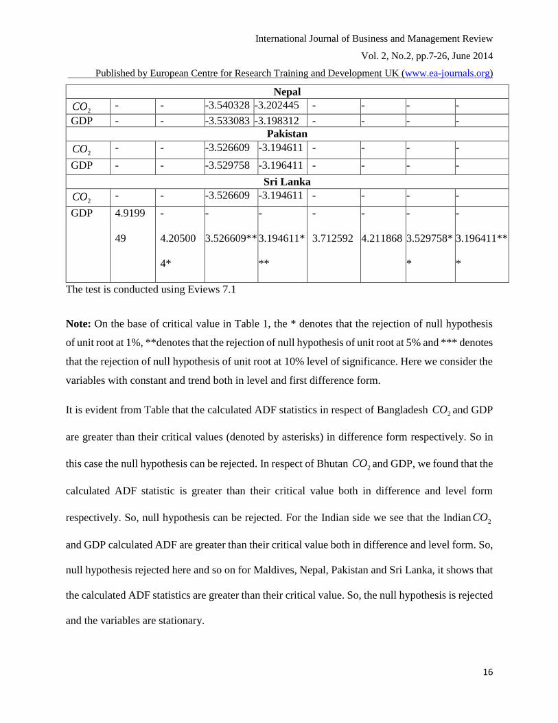
Table 1: Augmented Dickey-Fuller Unit Root Test Results

Level Form Difference Form

Variab

le

With Constant and Trend With Constant and Trend

Statistics

Critical Values Statistics

Critical Values 1% 5% 10% 1% 5% 10%

Bangladesh

2CO -

1.7230

54

-

4.21186

8

-3.529758 -3.196411 -

9.783222

-

4.211868

*

-

3.529758*

*

-

3.196411**

*

GDP 4.2579

90

-

4.20500

4*

-

3.526609*

*

-

3.194611**

*

-

0.876964

-

4.243644

-3.544284 -3.204699

Bhutan

2CO -

1.4751

81

-

4.20500

4

-3.526609 -3.194611 -

5.813915

-

4.211868

*

-

3.529758*

*

-

3.196411**

*

GDP 0.8132

14

-

4.21912

6

-3.533083 -3.198312 -

7.749178

-

4.211868

*

-

3.529758*

*

-

3.196411**

*

India

2CO 1.0237

85

-

4.21186

8

-3.529758 -3.196411 -

3.665813

-

4.211868

-

3.529758*

*

-

3.196411**

*

GDP 2.9502

38

-

4.20500

4

-3.526609 -3.194611 -

5.102512

-

4.211868

*

-

3.529758*

*

-

3.196411**

*

Maldives

2CO -

0.5716

52

-

4.23497

2

-3.540328 -3.202445 -

5.095165

-

4.234972

*

-

3.540328*

*

-

3.202445**

*

GDP -

1.6876

96

-

4.22681

5

-3.536601 -3.200320 -

6.657349

-

4.226815

*

-

3.536601*

*

-

3.200320**

*



Vol. 2, No.2, pp.7-26, June 2014


16

Nepal

2CO -

2.8498

25

-

4.23497

2

-3.540328 -3.202445 -

7.441555

-

4.211868

*

-

3.529758*

*

-

3.196411**

*

GDP -

1.6808

07

-

4.21912

6

-3.533083 -3.198312 -

6.560995

-

4.219126

*

-

3.533083*

*

-

3.198312**

*

Pakistan

2CO -

2.7016

88

-

4.20500

4

-3.526609 -3.194611 -

8.443667

-

4.211868

*

-

3.529758*

*

-

3.196411**

*

GDP -

2.2439

89

-

4.21186

8

-3.529758 -3.196411 -

4.285085

-

4.211868

*

-

3.529758*

*

-

3.196411**

*

Sri Lanka

2CO -

2.1166

80

-

4.20500

4

-3.526609 -3.194611 -

6.999085

-

4.211868

*

-

3.529758*

*

-

3.196411**

*

GDP 4.9199

49

-

4.20500

4*

-

3.526609**

-

3.194611*

**

-

3.712592

-

4.211868

-

3.529758*

*

-

3.196411**

*

The test is conducted using Eviews 7.1

Note: On the base of critical value in Table 1, the * denotes that the rejection of null hypothesis

of unit root at 1%, **denotes that the rejection of null hypothesis of unit root at 5% and *** denotes

that the rejection of null hypothesis of unit root at 10% level of significance. Here we consider the

variables with constant and trend both in level and first difference form.

It is evident from Table that the calculated ADF statistics in respect of Bangladesh 2CO and GDP

are greater than their critical values (denoted by asterisks) in difference form respectively. So in

this case the null hypothesis can be rejected. In respect of Bhutan 2CO and GDP, we found that the

calculated ADF statistic is greater than their critical value both in difference and level form

respectively. So, null hypothesis can be rejected. For the Indian side we see that the Indian 2CO

and GDP calculated ADF are greater than their critical value both in difference and level form. So,

null hypothesis rejected here and so on for Maldives, Nepal, Pakistan and Sri Lanka, it shows that

the calculated ADF statistics are greater than their critical value. So, the null hypothesis is rejected

and the variables are stationary.



Vol. 2, No.2, pp.7-26, June 2014


17

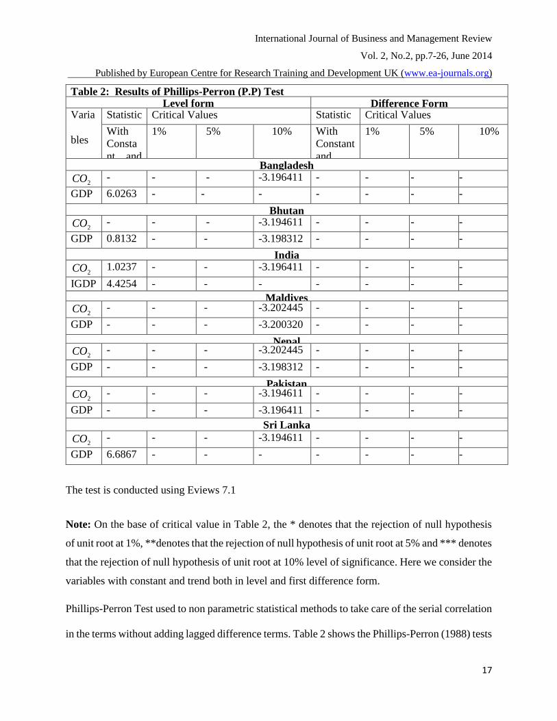
Table 2: Results of Phillips-Perron (P.P) Test Level form

Difference Form

Difference Form Varia

bles

Statistic

s

Critical Values Statistic

s

Critical Values

With

Consta

nt and

trend

1% 5% 10% With

Constant

and

trend

1% 5% 10%

Bangladesh

2CO -

1.7230

54

-

4.21186

8

-

3.529758

-3.196411 -

13.9047

6

-

4.21186

8*

-

3.529758*

*

-

3.196411*

**

GDP 6.0263

98

-

4.20500

4*

-

4.205004*

*

-

3.194611*

**

-

5.18601

6

-

4.21186

8*

-

3.529758*

*

-

3.196411*

**

Bhutan

2CO -

1.4751

81

-

4.20500

4

-

3.526609

-3.194611 -

5.79935

5

-

4.21186

8*

-

3.529758*

*

-

3.196411*

**

GDP 0.8132

14

-

4.21912

6

-

3.533083

-3.198312 -

7.84836

1

-

4.21186

8*

-

3.529758*

*

-

3.196411*

**

India

2CO 1.0237

85

-

4.21186

8

-

3.529758

-3.196411 -

3.70574

4

-

4.21186

8*

-

3.529758*

*

-

3.196411*

**

IGDP 4.4254

92

-

4.20500

4*

-

3.526609

**

-

3.194611*

**

-

5.14509

6

-

4.21186

8*

-

3.529758*

*

-

3.196411*

**

Maldives

2CO -

0.5716

52

-

4.23497

2

-

3.540328

-3.202445 -

25.7641

3

-

4.21186

8*

-

3.529758*

*

-

3.196411*

**

GDP -

1.6876

96

-

4.22681

5

-

3.536601

-3.200320 -

14.2238

0

-

4.21186

8*

-

3.529758*

*

-

3.196411*

**

Nepal

Nepal

2CO -

2.8498

25

-

4.23497

2

-

3.540328

-3.202445 -

7.41077

1

-

4.21186

8*

-

3.529758*

*

-

3.196411*

**

GDP -

1.6808

07

-

4.21912

6

-

3.533083

-3.198312 -

8.62115

9

-

4.21186

8*

-

3.529758*

*

-

3.196411*

**

Pakistan

2CO -

2.7016

88

-

4.20500

4

-

3.526609

-3.194611 -

8.47036

2

-

4.21186

8*

-

3.529758*

*

-

3.196411*

**

GDP -

2.2439

89

-

4.21186

8

-

3.529758

-3.196411 -

4.28508

5

-

4.21186

8*

-

3.529758*

*

-

3.196411*

**

Sri Lanka

2CO -

2.1166

80

-

4.20500

4

-

3.526609

-3.194611 -

6.95557

5

-

4.21186

8*

-

3.529758*

*

-

3.196411*

**

GDP 6.6867

38

-

4.20500

4*

-

3.526609

**

-

3.194611*

**

-

3.65398

2

-

4.21186

8

-

3.529758*

*

-

3.196411*

**

The test is conducted using Eviews 7.1

Note: On the base of critical value in Table 2, the * denotes that the rejection of null hypothesis

of unit root at 1%, **denotes that the rejection of null hypothesis of unit root at 5% and *** denotes

that the rejection of null hypothesis of unit root at 10% level of significance. Here we consider the

variables with constant and trend both in level and first difference form.

Phillips-Perron Test used to non parametric statistical methods to take care of the serial correlation

in the terms without adding lagged difference terms. Table 2 shows the Phillips-Perron (1988) tests



Vol. 2, No.2, pp.7-26, June 2014


18

results. It is evident from Table 2 that the calculated Phillip-Perron (P.P.) statistics in respect of

Bangladesh 2CO and GDP are greater than their critical values (denoted by asterisks) both in

difference and level form. In respect of Bhutan, India, Maldives, Nepal, Pakistan and Sri Lanka,

we see that the calculated P.P statistics in respect of 2CO and GDP are greater than their critical

value. So, the null hypothesis can be rejected and the data series are stationary.

Cointegration Results

Cointegration test clarifies that the existence of long run equilibrium relationship among the

variables. The cointegration technique is meant to calculate two statistics: Trace ( trace ) statistics

and the Maximum Eigen value (λ max ) statistics. The estimated results, particularly Maximum

Eigen value and Trace statistics are presented in the Table 3 which indicates that the statistics value

is greater than the critical value. This means that the hypothesis of no cointegration is rejected and

hence they are cointegrated. The Trace statistics and Maximum Eigen value tests indicate that

there is one cointegration eqn(s) at 5% level. This means that the variables among environmental

pollution (i.e. 2CO emission) and economic growth (i.e. GDP) have the long run relationships. So,

it is clear that there is one linear cointegration eqn(s) for each of the variables that there is one long

run relationship and liner deterministic trend among the variables.

More specifically, Table 3 shows that at 5 percent level of significance the likelihood ratios (trace

statistics) for the null hypothesis having one (r=1) cointegration (Bangladesh 52.09660, Bhutan

20.14684, India 31.24033, Maldives 30.52002, Nepal 26.51150, Pakistan 35.34613 and Sri Lanka

27.80299) are higher than their respective critical values (Bangladesh 15.49471, Bhutan 15.49471,

India 25.87211, Maldives 25.87211, Nepal 25.87211, Pakistan 25.87211 and Sri Lanka 15.49471).

At 5% level of significance, the maximum eigenvalue statisticsfor the null hypothesis having one



Vol. 2, No.2, pp.7-26, June 2014


19

cointegration (Bangladesh 50.89387, Bhutan 19.79190, India 26.51020, Maldives 21.64308,

Nepal 21.65528, Pakistan 31.54539 and Sri Lanka 25.86416) are higher than their respective

critical values (Bangladesh 14.26460, Bhutan 14.26460, India 19.38704, Maldives 19.38704,

Nepal 19.38704, Pakistan 19.38704 and Sri Lanka 14.26460). Hence, according to the likelihood

ratio and maximum Eigen value statistics tests, carbon emission and economic growth are

cointegrated. Thus, the long run equilibrium relationship among these series is cointegrated.

Table 3: Co-integration Results

Variable H0 H1 Trace

Statistics

5% Critical

value

Max. Eigen

value

5% critical

value

Hypothesis

Bangladesh

2CO GDP r=0 r=1 52.09660 15.49471 50.89387 14.26460 Ho: Rejected

r=1 r=2 1.202731 3.841466 1.202731 3.841466 H1: Accepted Bhutan

2CO

GDP

r=0 r=1 20.14684 15.49471 19.79190 14.26460 Ho: Rejected r=1 r=2 0.354942 3.841466 0.354942 3.841466 H1: Accepted

India

2CO

GDP

r=0 r=1 31.24033 25.87211 26.51020 19.38704 Ho: Rejected

r=1 r=2 4.730134 12.51798 4.730134 12.51798 H1: Accepted Maldives

2CO

GDP

r=0 r=1 30.52002 25.87211 21.64308 19.38704 Ho: Rejected

r=1 r=2 8.876940 12.51798 8.876940 12.51798 H1: Accepted

Nepal

2CO

GDP

r=0 r=1 26.51150 25.87211 21.65528 19.38704 Ho: Rejected

r=1 r=2 4.856219 12.51798 4.856219 12.51798 H1: Accepted Pakistan

2CO

GDP


Sri Lanka

2CO

GDP


Note: The Trace and Max. Eigen value test indicates that there is at least one (1) cointegrating

eqn(s) at 5% level of significance. Here ** denotes the rejection of the hypothesis at 0.05 level.



Vol. 2, No.2, pp.7-26, June 2014


20

Results of Error Correction Modeling

Engle and Granger (1987) showed that, if two variables (say X and Y) are individually integrated

of order one [i.e. I (I)] and cointegrated then there is possibility of a causal relationship in at least

one direction. That means cointegration with I (1) variables indicate the presence of Granger

causality but it does not indicate the direction of causality. The vector error correction model is

used to detect the direction of causality of long-run cointegrating vectors. Moreover, Granger

Representation Theorem indicates how to model a cointegrated series in a Vector Auto Regressive

(VAR) format. VAR can be constructed either in terms of level data or in terms of their first

differences [I (0)] with the addition of an error correction to capture the short run dynamics.

If the two variables are cointegrated, there must exist an error correction mechanism. This implies

that error correction model is associated with the cointegration test. The long term effects of the

variables can be represented by the estimated cointegration vector. The adjusted coefficient of

error correction term shows the long term effect and the estimated coefficient of lagged variables

shows the short term effect. Causality test among the variables are based on Error Correction

Model with first difference. Table 4 shows the results of error correction model of the variables.



Vol. 2, No.2, pp.7-26, June 2014


21

Table 4: Results of Error Correction Model

Coefficie

nt t F

Coefficie

nt t F

Bangladesh

2COfGDP 0.012022 [ 0.42823] 1.867654 GDPfCO 2

51.52446

**

[

7.74284]

50.44211

Bhutan

2COfGDP 0.002749 [ 0.23656] 0.364334

GDPfCO 2 -

22.31243

**

[-

4.80641]

8.089451

India

[ 0.23656]

[-4.80641]

2COfGDP -0.002613 [-0.43108] 9.506284 GDPfCO 2 -

10.77139

**

[-

4.42385]

17.17979

Maldives

2COfGDP -

0.361661

**

[-3.72978] 7.365691 GDPfCO 2 -79.42380 [-

0.92433]

5.569285

Nepal

2COfGDP -

0.197094

[-

1.91152]

[-

1.91152]

1.160219

GDPfCO 2 -

106.6725

**

[-

3.68314]

3.250268

Pakistan

2COfGDP -0.112020 [-

0.57248]

4.644593 GDPfCO 2 131.6173 [

1.47971]

2.041946

Sri Lanka

2COfGDP 0.000134 [ 0.06242] 0.656019 GDPfCO 2 -

3.472699

**

[-

3.81311]

16.65960

Note: ** denotes the rejection of the hypothesis at 5% level of significance. The ** values are

statistically significant and shows the estimated coefficient of lagged variables. Values in the third

brackets are t-statistics.

Table 4 shows the significance of Error Correction Term (ECT) for carbon dioxide ( 2CO ) emission

and economic growth (GDP) of SAARC countries. It is evident from the Table that the error

correction term (ECT) is significant for the country Bangladesh, India, Nepal, Bhutan and Sri

Lanka in term of GDP, i.e. in these country GDP causes 2CO for the long term perspective. But

in Maldives the ECT is significant in respect of 2CO emission and for Pakistan we did not find

the significance of ECT.



Vol. 2, No.2, pp.7-26, June 2014


22

CONCLUSION

This paper examines the long-run causal relationships between 2CO emissions and economic

growth in SAARC countries during the period of 1972-2012. We apply cointegration and VECM

to evaluate the relationship. Empirical results suggest that a long run relationship exist between

2CO emissions and economic growth in SAARC countries. The application of the cointegration

based Granger Causality test found that there is a long run (short run also) relationship between

economic growth and 2CO emissions that is energy consumption granger causes 2CO emissions

and economic growth (GDP). Hence, the long run income elasticity of carbon emissions are greater

than the short run income elasticity of carbon emissions, which implies that income (GDP) leads

to greater carbon dioxide emissions in the SAARC countries. That is why the significant and

positive impact of energy consumption is crucial for economic growth, but the rapid pace of 2CO

emissions requires the adoption of environment friendly developed technology or alternative

sources of energy for the protection of environment in seven SAARC countries.

REFERENCES

Amin, S. B., Ferdaus, S.S., and Porna, A.K., (2012), Causal Relationship among Energy Use, CO2

Emissions and Economic Growth in Bangladesh: An Empirical Study, World Journal of Social

Sciences, 2, 4, 273 – 290.

Apergis, N., and D. Chapman, (1999), 2CO emissions, energy use, and output in Central America,

Energy Policy, 37, 3282-3286



Vol. 2, No.2, pp.7-26, June 2014


23

Andreoni, S., and Galmarini, (2012), Decoupling economic growth from carbon dioxide

emissions: A decomposition analysis of Italian energy consumption,

http://dx.doi.org/10.1016/j.energy.

Asafu-Adjaye, J., (2000), The relationship between energy consumption, energy prices and

economic growth: Time series evidence from Asian developing countries, Energy Economics, 22,

615-625.

Bhattacharyya, R., and T. Ghoshal, (2009), Economic growth and 2CO emissions, Environmental

Development and Sustainability, http:// DOI 10.1007/s10668-009-9187-2

Bloch, H. et al. (2012), Coal consumption, 2CO emission and economic growth in China:

Empirical evidence and policy responses, Energy Economics, 34, 518-528.

Böhm, D.C., (2011), Economic Growth, Energy Demand and the Environment – Empirical

Insights Using Time Series and Decomposition Analysis, www.weissensee-verlag.de

Boopen, S. and Harris, N., (2012), Energy use, Emissions, Economic growth and Trade: Evidence

from Mauritius, ICTI 2012, ISSN: 16941225, [email protected]

Chebbi, H. E. and Boujelbene, Y., (2008), CO2 emissions, energy consumption and economic

growth in Tunisia, 12th Congress of the European Association of Agricultural Economists – EAAE

2008.

Dantama, Y. U., and Inuwa, N., 2012, A Granger-Causality Examination of the Relationship

between Energy Consumption & Economic Growth in Nigeria, Journal of Economics,

Commerce and Research (JECR) ISSN 2278-4977, 2, 2, 14 – 24


http://dx.doi.org/10.1016/j.energy.2012.05.024

http://www.weissensee-verlag.de/


Vol. 2, No.2, pp.7-26, June 2014


24

Dickey, D.A., and W.A. Fuller 1981, Distribution of the estimators for the autoregressive time

series with a unit root, Econometrica, 49, 1057-1072.

Dhungel, K. R., (2008), A Causal Relationship Between Energy Consumption and Economic

Growth in Nepal, Asia-Pacific Development Journal, 15, 1.

Engle, R.F., and C.W.J. Granger, (1987), Cointegration and error correction-representation,

estimation and testing, Econometrica, 55, 251-276.

Grossman, G.M, and A.B. Krueger, (1995), Economic growth and the environment, Quarterly

Journal of Economics, 110, 2, 353-377

Hatzigeorgiou, E., Polatadis, H., and Haralambopoulos, D., (2013), Modeling the Relationship

among Eenrgy demand, CO2 emission and Economic Development: A Survey for the case of

Greece, Global NEST Journal, XX, X, XX-XX.

Hey, Qazi, M.A., Mashkoor, Masood Siddiqui, (2010), Growth and Energy Nexus: An Empirical

Analysis of Bangladesh Economy, European Journal of Social Science, 15, 2.

Holtz-Eakin, D. and T.M. Selden, (1995), Stocking the fires? 2CO Emissions and Economic

Growth, Journal of Public Economics, 57, 85-101.

Jalil, A., and S.F. Mahmud, (2009), Environment Kuznets curve for 2CO emissions: a cointegration

analysis, Energy Policy, 37, 5167-5172, http://dx.doi.org/101016/j.enpol.

Jinke, L., and Zhongxue, L., (2011), A Causality Analysis of Coal Consumption and Economic

Growth for China and India, Natural Resources, 2, 54-60, http://www.scirp.org/journal/nr



Vol. 2, No.2, pp.7-26, June 2014


25

Lau, L.C., Tan, K.T., and A.R., Mohamed, (2009), A Comparative study of the energy policies in

Japan and Malaysia in fulfilling their nation’s obligations towards the Kyoto protocol, Energy

Policy, 37, 4771-4780. http://dx.doi.org/10.1016/j.enpol

McKinsey Global Company, (2008), The carbon productivity challenge: Curbing climate change

and sustaining economic growth. The McKinsey Quarterly, 7, 2-33.

Muhammad, S., and Smile, D., (2012), Revisiting the Relationship between Coal Consumption

and Economic Growth: Cointegration and Causality Analysis in Pakistan, Applied Econometrics

and International Development, 12, 1.

Muhittin Kaplan, M.,Ozturk, I., and Kalyoncu, H., (2011), Energy Consumption and Economic

Growth in Turkey : Cointegration and Causal Analysis, Romanian Journal of Economic

Forecasting – 2/2011

Nain,Z., Ahmad, W., and Kamaiah, B., (2013), Economic Growth, Electricity Consumption and

CO2 Emissions in India: A Disaggregated Causal Analysis.

Noor, S., and M. W Siddiqi, (2010), Energy Consumption and Economic Growth in South Asian

Countries: A Co-integrated, International Journal of Human and Social Sciences, 5, 14.

Ong, S.M., and sek, S.K., (2013), Interactions between Economic Growth and Environmental

Quality: Panel and Non-Panel Analyses, Applied Mathematical Sciences, 7, 14, 687 – 700

Ozturk, I. and uddin, G.S., (2011), Causality Among Carbon Emission, Energy Consumption and

Growth in India, Economic Research - Ekonomska Istrazivanja, 25, 3, 753

Phillips-Perron, (1988), Testing for Unit root in Time Series Regression, Biometrica, 75, 335-346.

http://dx.doi.org/10.1093/biomet/75.2.335



Vol. 2, No.2, pp.7-26, June 2014


26

Shaari, M.S., Hussain, N.E., and Ismail, M.S., (2012), Relationship between Energy

Consumption and Economic Growth: Empirical Evidence for Malaysia, www.business-systems-

review.org, 2, 1.

The World Bank, (2007), Growth and 2CO emissions: how do different countries fare,

Environment Department, Washington,

http://wwwds.worldbank.org/external/default/WDSContent/IB/2007/12/05/000020953_2007120

5142250/Renderd/PDF/417600EDP01130Growth0and0co201PUBLIC1.pdf

The World Bank, (2013), GDP and 2CO emissions of different countries from 1972-2012,

World Development Indicators Statistics

Tiari, A.K., (2011), Energy Consumption, CO 2 Emissions and Economic Growth: Evidence

from India, Journal of International Business and Economy, 12, 1, 85-122.

Wahid, I.N., Aziz, A.A., and Mustapha, N. H. N., (2013), Energy Consumption, Economic

Growth and CO2 emissions in Selected ASEAN Countries, PROSIDING PERKEM VIII, JILID,

2, 2013, 758 – 765


http://www.business-systems-review.org/

http://www.business-systems-review.org/

CARBON EMISSION AND ECONOMIC GROWTH OF SAARC …

Documents

Transcript of CARBON EMISSION AND ECONOMIC GROWTH OF SAARC …