1

Economic analysis of condition monitoring systems for offshore wind

turbine sub-systems

Allan May

1*, David McMillan

2, Sebastian Thöns

3

1

Centre for Doctoral Training in Wind Energy Systems, University of Strathclyde, 204

George Street, Glasgow, UK 2

Institute of Energy and Environment, University of Strathclyde, Glasgow, UK 3

Department of Civil Engineering, Technical University of Denmark, Brovej, Kgs. Lyngby,

Denmark *allan.may@strath.ac.uk

Abstract: The use of condition monitoring systems on wind turbines has increased dramatically in

recent times. However, their use is mostly restricted to vibration based monitoring systems for the

gearbox, generator and drive train. A survey of commercially available condition monitoring

systems and their associated costs has been undertaken and is presented for the blades, drive train,

tower and foundation.

This paper considers what value can be obtained from integrating these additional systems into the

maintenance plan. This is achieved by running simulations on an operations and maintenance model

for a wind farm over a 20 year life cycle. The model uses Hidden Markov Models to represent both

the actual system state and the observed condition monitoring state. The CM systems are modelled

to include reduced failure types, false alarms, detection rates and 6 month failure warnings.

The costs for system failures are derived, as are possible reductions in costs due to early detection.

The drive train has additional sensors to increase the overall CM system detection rate. The

detection capabilities of the CM systems installed on blades, tower and foundation is investigated

and the effects on operational costs are examined. Likewise, the number of failures detected 6

months in advance by the CM systems is modified and the costs reported.

Nomenclature

AE Acoustic emission

C Cost

CAPEX Capital expenditure

CBM Condition based maintenance

CM Condition monitoring

CMS Condition monitoring system

DT Downtime

f Number of failures

E Emission state matrix

HMM Hidden Markov model

LP Lost production

NPV Net present value

O&M Operations and maintenance

OPEX Operational expenditure

P State transition matrix

PM Preventative maintenance

r Discount rate

R Effectiveness of condition monitoring systems

2

ROI Return on investment

SCADA Supervisory control and data acquisition

SHM Structural health monitoring

U Probability of failure

V Reliability of condition monitoring systems

t Time period under investigation

T Fixed period of time

λ Failure rate

µ Repair rate

Subscript

E Energy production

f Component failure

fa False alarm

I Installation

L Labour price

V Vessel

RP Replacement parts

Superscript

+ Condition monitoring equipment is used

k Number of components

y Number of years

1. Introduction

Wind energy has enjoyed a large growth in recent years as countries around the world seek to exploit

renewable resources. Offshore wind projects have been part of this expansion but access related issues

such as remote locations, specialist access equipment and extreme weather has led to operation and

maintenance (O&M) costs which are up to five times that of onshore [1]. O&M costs are a sizeable part of

the total costs associated with an offshore wind project - up to 30% of the energy generation cost [2].

As such, there have been many investigations to discover ways of reducing O&M costs. Increased

utilisation of SCADA data and condition monitoring (CM) systems have allowed for a shift in

maintenance pattern.

Maintenance plans can be divided generally into preventative and corrective maintenance.

Corrective maintenance occurs after a failure has occurred. Preventative maintenance (PM) is used to

minimise downtime by servicing or component replacement. This can be in the form of scheduled

maintenance, where servicing occurs based on calendar intervals, or condition based maintenance (CBM),

where maintenance actions are triggered by the actual condition of a component.

CBM theoretically allows for a reduction in both downtime and maintenance operations. The

majority of CM systems are vibration based and focused on the drive train of wind turbines - the generator,

3

gearbox and associated bearings - as these components historically have large amounts of downtime per

failure [3] and can be monitored effectively [4], [5].

Several studies examine the possible benefit of CM drive train systems and the majority of these

show a return on investment (ROI) of the monitoring equipment [6]–[8]. These studies utilise simplified

CM systems which show direct correlation between the system and output. The system will always inform

the user ahead of time of any impending failure mode.

Different types of imperfections have been introduced to CM systems and their effects on O&M

costs have been examined [2], [9]–[13]. Typically, the time until the CM system ROI becomes positive

increases in these studies and in some cases the use of CM systems isn‟t economically valid. These studies

almost all exclusively use only a vibration based condition monitoring system.

García Márquez et al. [14] shows some CM systems analysing parts of the wind turbine other than

the drive train are available commercially and some further experimental CM techniques show promise.

These include systems for monitoring foundations, offshore foundation areas (to examine scour) and

blades.

There has been limited work examining the economic benefit of Structural Health Monitoring (SHM)

systems. A work by Thöns, Faber and Rücker [15] dedicated to quantifying the value of SHM for offshore

wind turbine structures shows expected benefits which could be associated to a positive ROI for the

majority of scenarios examined. Preliminary work has been completed investigating the use of multiple

monitoring systems. The work of Thöns and McMillan [16] examines the use of CM systems and an SHM

system for offshore foundations. May and McMillan [17] take a broad approach to the use of CM systems

for all subsystems.

This paper will look at extending the studies of economic benefit currently conducted for vibration

drivetrain CM studies to other types and subsystems. These alternative commercially available CM

systems are introduced in Section 2 and in Section 4 a cost study of the capital expenditure (CAPEX) and

operational expenditure (OPEX) of these systems is shown. The remainder of the Section 4 introduces an

O&M cost model and the differences between how PM and CBM O&M costs are realised. The difference

between strategies includes possible reductions in component costs, downtime and access costs. Section 3

details how subsystems and CM systems are modelled. A wide range of factors are included in the CM

modelling: overall detection rate of failures; increase in failure detection rate with multiple CM systems;

fault class reduction due to advanced detection; advanced failure detection of 6 months or more; and false

alarms.

4

2. Condition Monitoring Systems

The condition monitoring systems described below have been selected due to the possibility of them

delivering real-time information to a turbine operator and being included in a regular SCADA or existing

CM system data stream. The majority of these technologies have been chosen from the studies of CM

systems by Ciang, Lee and Bang [18] and Crabtree [19].

2.1 Oil Analysis

Oil performs essential functions for gearbox, generator and bearings and is monitored with several

SCADA channels dealing with temperature, pressure and oil filter status [20]. By further analysing the

content, quality and the debris suspended within lubricating oil much can be learned about a component's

condition. There have been many approaches suggested for analysing oil. However, the majority of these

methods are offline and as such cannot be conducted in real time [21], [22].

Dielectric current sensors can monitor a change in the electromagnetic properties of oil and can

detect both types (ferrous and non-ferrous) and an estimation of the amount of debris. Another technique

uses magnets to attract ferrous particles onto a screen. Once the screen is full it is then flushed. The time

between flushes are recorded to give an indication of oil debris content.

2.2 Vibration

Vibration based CM systems have been widely adopted for monitoring wind turbine drive trains.

Accelerometers are used to measure the forces being applied to the component and these are trended over

time with frequency. Techniques on how to analyse this vibration data for wind turbines are given by

Hameed et al. [23].

However, vibration systems have also been utilised for other applications including blade and tower

monitoring. The monitoring techniques and methods are in some aspects similar to drive train CM systems

[24] but the data are sampled at lower frequencies. The vibration data can be utilized to calculate damage

indicators which can be based on the natural frequencies and mode shapes of the structure and foundation.

Such damage indicators facilitate the detection and the localization of structural damages.

2.3 Optical Fibre

Optical fibre systems have been demonstrated on wind turbine blades to measure strain using two

distinct methods. In one method, the attenuation of light as it travels through the fibre is measured. It is

from measuring this deviation that strain can be determined. The second method uses fibre Bragg gratings.

A Bragg grating is an etching in an optical fibre that reflects a certain wavelength of light. If the grating is

subject to strain then the wavelength returned to the measuring point alters. As multiple gratings can be

used on the same fibre and are highly sensitive, fibre Bragg grating allow for blade impacts to be detected.

5

Some optical systems are available for retrofitting onto existing turbines with minimal modification

to the turbine. However, some systems require that the fibres are impregnated into the blades during the

curing phase. This obviously requires special blades be manufactured. One study suggests that having

fibres impregnated may actually be advantageous to ensure that the curing of blades is completed properly

[25]. There is the possibility to realise time and energy savings in the manufacturing process using this

technique.

2.4 Acoustic Emission

Acoustic emission (AE) involves the use of piezoelectric sensors to record the release of stored

elastic energy during cracking and deformation. The energy released is in the form of high energy waves

which are outside the audible range. The signals can be categorised by their amplitude into the type of

damage occurring and when several sensors are used a location can be determined. AE events have been

shown to 'cluster' around the ultimate failure point.

3. Operation Modelling

3.1 Markov Processes

The wind is a stochastic process and complex loadings lead to complex component failure patterns.

Various methodologies have been implemented to examine the failure process and the effectiveness of

various O&M plans. Gamma processes [26], P-F Curves [12] and Markov chains have been widely used to

represent wind turbine failure patterns. Simulations are used instead of analytical expressions to account

for these wind complexities.

Failure rates, λ, are commonly used to express the number of failures, f, expected to occur over a

fixed time period, T, usually a year. These can be converted into a percentage chance of failure, U, for any

different given period of time, t. These are shown in Equations (1) and (2). Failure rates can be used to

populate a state transition matrix, P, used in Markov processes as in Equation (3). In this equation, the

ability of the system to transition from a failed state to a repaired one is given as a percentage, µ.

(1)

( ) (2)

[

] (3)

*

+ (4)

3.2 Condition Monitoring System

6

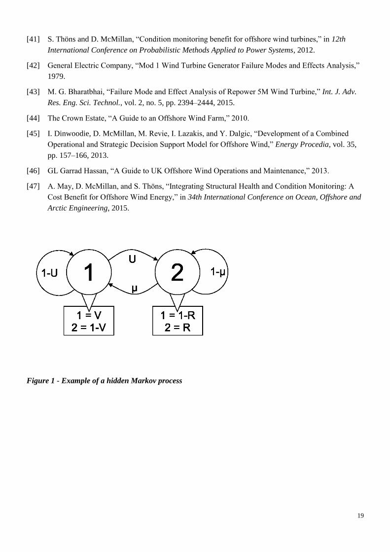
Hidden Markov Models (HMM) show an observed state instead of the actual state of the system.

The observable state can be different to the actual condition of the system. This is shown graphically in

Figure 1. In HMM it is the emissions matrix, E, that contains the probabilities of what is observed by the

operator and is shown in Equation (4). The emissions matrix is used to define how accurately the condition

monitoring system reports failures and how frequently it returns false results.

Condition monitoring effectiveness is a concept used in several works [8], [9], [17]. The

effectiveness of the condition monitoring system to detect a failure before it occurs is stored as a

percentage, R, in the emissions matrix. As the value of R increases then there is an increased likelihood

that the system will detect a failure before a turbine shutdown occurs. The effectiveness is referred to in

this paper as CM detection rate. Weiss [27] gives detection rates for the GE Bentley Nevada ADAPT wind

system and these are shown in Table 1.

In this paper, multiple CM systems that observe different properties are added to the same sub-

system. For example, Nie [28] states that multiple oil sensors would provide greater accuracy of condition

for components. These have been modelled as parallel systems as shown in Tavner [29].

The reliability of the CM system is defined as V. This is the ability of the CM system to correctly

show that the system is operating while it is indeed operating correctly. The lower the percentage, the

greater chance of the system showing an erroneous failed state. The effects of CM system reliability have

been investigated by the authors in a previous study [17] and for this paper the reliability has been fixed at

99%. Takoutsing et al. [30] state that false warnings and alarms occur frequently and at 99% this equates

to 4 false alarms per turbine per year.

These two properties, V and R, allow for false positives, false negatives and CM system failures to

be accounted for.

Table 1 CM system detection rates

Subassembly Detection Rate

Gearbox 50%

Generator 80%

Drive Train (incl. Main Bearing and Coupling) 40%

3.3 Failure Analysis

A model has been constructed that represents turbines as structures with 13 sub-assemblies. This

follows the taxonomy as originally used in WMEP programme in Germany within the “250 MW Wind”

7

project covered in the annual Wind Energy Reports from ISET [31] and explored for possible offshore

developments by Faulstich, Hahn and Tavner [32]. A notable exception to this taxonomy is the addition of

a subsystem representing the offshore foundation. The layout of the O&M model and flow of data is

shown in Figure 2. This includes the turbine taxonomy and the required information for each subsystem.

For clarity, the “Support and Housing” subsystem has been renamed “Tower and Access”.

A wind farm is constructed from multiple independent turbine structures. Failure rates are taken

from operation reports from 2007-2009 for Egmond aan Zee offshore wind farm [33]. The farm consists of

36 Vestas V90 3 MW turbines which have the number of turbine stops (regardless of whether on site

intervention was required or not) and downtime per subsystem reported. The farm is located between 10

and 18 km from the coast of the Netherlands in the North Sea. These failure rates are modified as by

Dinwoodie, Quail and McMillan [34] which uses the number of recorded personnel visits to the wind farm

to modify the failure rate as a proportion of total stops. The failure rate and downtime are divided into

'Major' and 'Minor' failures for each subsystem are based on the onshore ratio taken again from Faulstich,

Hahn and Tavner [32]. The work describes that the „Minor‟ class of failures account for approximately 75%

of all failures but only 5% of the downtime. Conversely, the „Major‟ class is 25% of total failures and 95%

of the downtime. „Minor‟ faults are described as those taking less than 24 hours to clear. A scheduled

maintenance service occurs at a rate of 1 visit per turbine per year.

During 2008 and 2009 all the gearboxes at Egmond aan Zee were replaced due to technical issues

[35] and to improve availability. This will have altered the failure rates and downtime of the gearbox to

make it unrepresentative of the current reliability. There are not many other sources available of actual

offshore operation data to directly compare this to. Besnard [36] shows a breakdown of the total downtime

for the Horns Rev for 2009-2010 which excludes its own serial failures and has approximately 5 failures

per year compared to 6 for Egmond aan Zee. Horns Rev consists of 80 Vestas V80 2 MW turbines located

approximately 18 km off the coast of Denmark. The two wind farms are compared in Table 2 excluding

ambient fault downtime. For use in the model the total hours of downtime assigned for gearboxes is

reduced by 50% so that the estimated downtime becomes 38.59% of total downtime.

8

Table 2 Comparison of Egmond aan Zee and Horns Rev Wind Farm

Subassembly Estimated downtime per subsystem

Egmond aan Zee Horns Rev

Blade system 1.72% 8.00%

Brake system 0.17% 1.00%

Control system 9.56% 8.00%

Converter 3.67% 9.00%

Electrical 2.05% 12.00%

Gearbox 55.69% 33.00%

Generator 15.12% 9.00%

Pitch system 4.96% 6.00%

Scheduled service 5.34% 11.00%

Yaw system 0.88% 2.00%

Structure 0.44% 0.00%

Grid 0.40% 1.00%

Smith establishes that the majority of components experience periods of infant mortality, 72%, and

only a small amount show wear out at the end of their life [37]. The failure rates are used for the first 3

years before being reduced for a further 2 years using a Weibull function with a shape parameter of 0.8

[38].

3.4 Modelling Operations Strategies

The model is solved by simulation. The model generates an operational and observed state for every

turbine subsystem based on comparing a randomly generated uniformly distributed number to the

percentages contained in the P and E matrices. This is repeated for each turbine in the farm and for each

operational year on a monthly timescale. Each failure event type has associated repair, downtime and fault

class specifying the required vessels.

The PM strategy cost is based entirely on the modified data from Egmond aan Zee. It assumes an

annual service per turbine, that all failures are classified as CM system unobserved failures, and there are

no false alarms. The wind farm does have a SCADA system but these and weather based observations

aren‟t included in the cost model as these variables are already a part of the annual downtime values in the

operation reports.

For the CBM strategy, an algorithm compares the operational and observed states and notes any

differences. These are then classified as CM observed failure events, CM unobserved failure events and

false alarms. CM observed failures in certain instances have reduced failure classifications and costs. An

annual service per turbine is also included.

O&M costs for both a PM and CBM strategies are calculated using this information and the cost

model outlined below. In the model, each turbine is simulated independently at least for 4000 Markov

9

years where convergence is observed. The resulting total failures are then averaged. This gives the costs

for that operational year.

4. Cost Modelling

The annual operating and maintenance costs are calculated from adding the costs incurred from 4

items: replacing parts; the lost energy production; the logistics costs including crew and vessel hire; and

the installation and use of CM systems.

The costs for each year are levelised to represent the Net Present Value (NPV) of the lifetime

operating costs. NPV is shown in Equation (6) where a discount rate, r, of 8.2% is used [39] and cost of

year i is defined by CO&M. Additionally, all costs were adjusted for inflation to 2015 – where other years

are quoted, a value of 2.2% has been used.

∑ ( )

( ) (6)

4.1 Replacing Components

A failure in a subsystem will incur a cost for part replacement. The cost depends on the severity of

the failure and damage caused by the failure, Cf. The cost of replacement parts, CRP, is summed for each

subsystem, k, as seen in Equation (7).

If the failure is detected in advance by the CM system then in some cases the replacement costs, ,

can be lowered if the damage isn't as severe. This alternate cost, , is shown in Equation (8).

The costs for turbine replacement parts are compiled from the work of Martin-Tretton et al. [40].

This gave average 2010 list prices for 2.1 to 3 MW onshore turbines. The additional cost of marinisation

for offshore use was found using a factor of 1.27 [34]. The cost of the repairs for the tower and foundation

are taken from the work of Thöns and McMillan [41].

A thorough FMEA of a wind turbine [42] was used to determine which corresponding components

from the parts list were replaced in relevant major and minor subsystem failures both with and without

CM detection. Due to the age of the previous study it was checked against a less complete but more

modern FMEA for a Repower 5MW turbine [43]. There are few sources for the costs of components so

major failures were compared to the new price of subsystems from estimates by the Crown Estate [44] and

Williams, Crabtree and Hogg [11].

∑ ( ) (7)

∑ ( ( )

( )) (8)

10

4.2 Lost Production

A turbine cannot produce energy while it is not operational or offline for maintenance. The longer

the downtime (DT) associated with a failure then the greater the lost production (LP). In the cost benefit

analysis the LP is used to represent income that would have been earned if the turbine was operating.

The cost of lost production, CLP, is the sum of the DT from all subsystem failures, Tf, multiplied by

the energy production cost, CE, shown in Equation (9). This is the cost of energy in the market (including

obligation tariffs prices per unit) multiplied by the capacity factor.

If a CM system can detect a failure in advance then the DT will be reduced as logistic operations can

be started in advance of the failure causing a shutdown. This reduced downtime value is indicated by .

As mentioned previously, there is the possibility of receiving false alarms. A critical subsystem alarm will

result in a turbine shut down until a trained technician can inspect the component or further analysis can be

performed on the data. The time taken to resolve false alarms, Tfa, is added to the DT in Equation (10)

along with the alternative cost of lost production, , when using a CM system. No average downtime

associated with false alarms was available so therefore 24 hours is used to represent the DT in the model

as an approximation.

∑ ( ) (9)

∑ ( ( )

( ) ( )) (10)

4.3 Operations Costs

Technicians and appropriate vessels need to be used to complete resets and to replace parts. Each

failure mode is assigned a failure category. This category relates to the severity of the failure. A high

category failure indicates that large parts will need to be replaced requiring both a crew access vessel and a

crane vessel. It also requires a large logistics time and a crew in excess of 7. Conversely, low category

failures can be organised more quickly as they utilise only a crew access vessel and a small crew. If the

CM equipment allows for a significant reduction in replacement components then the fault class may also

be reduced.

The installation costs, CI, are given in Equation (11). The costs of vessel hire, CV, are based on

Bjerkseter and Ågotnes [39] and the labour costs per hour, per crew member, CL, are £90 as used by

Williams, Crabtree and Hogg [11]. The total number of hours required to complete repairs are and logistic

hours required to mobilise the vessel are estimated from a commercial report. Vessels are hired by the day

but the crew are hired by the hour including travel time to the farm based on the distance from shore and

the speed of the vessel. The annual service scheduled serviced that is mentioned in Section 3.4 is included

in this variable for both the PM and CBM cost models.

11

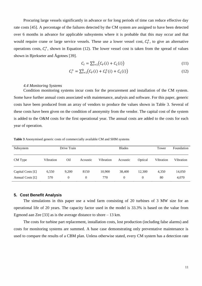
Procuring large vessels significantly in advance or for long periods of time can reduce effective day

rate costs [45]. A percentage of the failures detected by the CM system are assigned to have been detected

over 6 months in advance for applicable subsystems where it is probable that this may occur and that

would require crane or large service vessels. These use a lower vessel cost, , to give an alternative

operations costs, , shown in Equation (12). The lower vessel cost is taken from the spread of values

shown in Bjerkseter and Ågotnes [39].

∑ ( ( ) ( )) (11)

∑ ( ( )

( ) ( )) (12)

4.4 Monitoring Systems

Condition monitoring systems incur costs for the procurement and installation of the CM system.

Some have further annual costs associated with maintenance, analysis and software. For this paper, generic

costs have been produced from an array of vendors to produce the values shown in Table 3. Several of

these costs have been given on the condition of anonymity from the vendor. The capital cost of the system

is added to the O&M costs for the first operational year. The annual costs are added to the costs for each

year of operation.

Table 3 Anonymised generic costs of commercially available CM and SHM systems

Subsystem Drive Train Blades Tower Foundation

CM Type Vibration Oil Acoustic Vibration Acoustic Optical Vibration Vibration

Capital Costs [£] 6,550 9,200 8150 10,900 38,400 12,300 4,350 14,050

Annual Costs [£] 570 0 0 770 0 0 80 4,070

5. Cost Benefit Analysis

The simulations in this paper use a wind farm consisting of 20 turbines of 3 MW size for an

operational life of 20 years. The capacity factor used in the model is 33.3% is based on the value from

Egmond aan Zee [33] as is the average distance to shore – 13 km.

The costs for turbine part replacement, installation costs, lost production (including false alarms) and

costs for monitoring systems are summed. A base case demonstrating only preventative maintenance is

used to compare the results of a CBM plan. Unless otherwise stated, every CM system has a detection rate

12

of 80%, excluding the system for the vibration drive train which is as noted in Table 1. Likewise, the

percentage of faults that are detected more than 6 months in advance to access lower vessel costs is set at

10% of all detected faults unless otherwise noted.

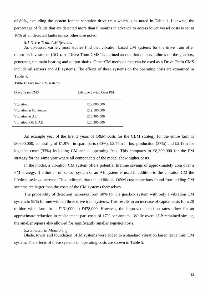
5.1 Drive Train CM Systems

As discussed earlier, most studies find that vibration based CM systems for the drive train offer

return on investment (ROI). A „Drive Train CMS‟ is defined as one that detects failures on the gearbox,

generator, the main bearing and output shafts. Other CM methods that can be used as a Drive Train CMS

include oil sensors and AE systems. The effects of these systems on the operating costs are examined in

Table 4.

Table 4 Drive train CM systems

Drive Train CMS Lifetime Saving Over PM

Vibration £12,000,000

Vibration & Oil Sensor £19,100,000

Vibration & AE £18,900,000

Vibration, Oil & AE £20,300,000

An example year of the first 3 years of O&M costs for the CBM strategy for the entire farm is

£6,600,000, consisting of £1.97m in spare parts (30%), £2.47m in lost production (37%) and £2.19m for

logistics costs (33%) including CM annual operating fees. This compares to £8,300,000 for the PM

strategy for the same year where all components of the model show higher costs.

In the model, a vibration CM system offers potential lifetime savings of approximately £6m over a

PM strategy. If either an oil sensor system or an AE system is used in addition to the vibration CM the

lifetime savings increase. This indicates that the additional O&M cost reductions found from adding CM

systems are larger than the costs of the CM systems themselves.

The probability of detection increases from 50% for the gearbox system with only a vibration CM

system to 98% for one with all three drive train systems. This results in an increase of capital costs for a 20

turbine wind farm from £131,000 to £478,000. However, the improved detection rates allow for an

approximate reduction in replacement part costs of 17% per annum. While overall LP remained similar,

the smaller repairs also allowed for significantly smaller logistics costs.

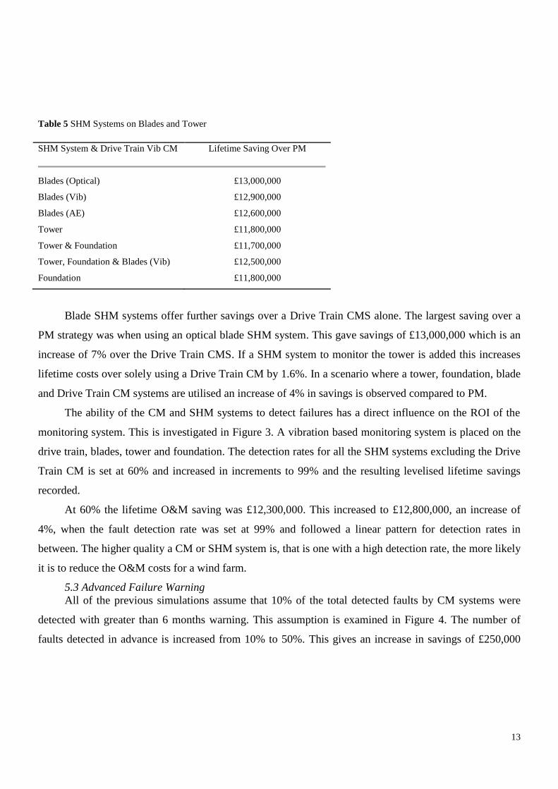
5.2 Structural Monitoring

Blade, tower and foundation SHM systems were added to a standard vibration based drive train CM

system. The effects of these systems on operating costs are shown in Table 5.

13

Table 5 SHM Systems on Blades and Tower

SHM System & Drive Train Vib CM Lifetime Saving Over PM

Blades (Optical) £13,000,000

Blades (Vib) £12,900,000

Blades (AE) £12,600,000

Tower £11,800,000

Tower & Foundation £11,700,000

Tower, Foundation & Blades (Vib) £12,500,000

Foundation £11,800,000

Blade SHM systems offer further savings over a Drive Train CMS alone. The largest saving over a

PM strategy was when using an optical blade SHM system. This gave savings of £13,000,000 which is an

increase of 7% over the Drive Train CMS. If a SHM system to monitor the tower is added this increases

lifetime costs over solely using a Drive Train CM by 1.6%. In a scenario where a tower, foundation, blade

and Drive Train CM systems are utilised an increase of 4% in savings is observed compared to PM.

The ability of the CM and SHM systems to detect failures has a direct influence on the ROI of the

monitoring system. This is investigated in Figure 3. A vibration based monitoring system is placed on the

drive train, blades, tower and foundation. The detection rates for all the SHM systems excluding the Drive

Train CM is set at 60% and increased in increments to 99% and the resulting levelised lifetime savings

recorded.

At 60% the lifetime O&M saving was £12,300,000. This increased to £12,800,000, an increase of

4%, when the fault detection rate was set at 99% and followed a linear pattern for detection rates in

between. The higher quality a CM or SHM system is, that is one with a high detection rate, the more likely

it is to reduce the O&M costs for a wind farm.

5.3 Advanced Failure Warning

All of the previous simulations assume that 10% of the total detected faults by CM systems were

detected with greater than 6 months warning. This assumption is examined in Figure 4. The number of

faults detected in advance is increased from 10% to 50%. This gives an increase in savings of £250,000

14

from £11.91m to £12.16m which is an increase of 2% for a scenario where only a Drive Train CMS is

used.

5.4 Additional Analysis

A report from GL Garrad Hassan, The Crown Estate and Scottish Enterprise gives more recent

offshore availability figures as between 90 and 95% [46]. This is much higher than the average figures

reported from Egmond aan Zee of 80% for the 3 years up to 2009. The simulation with the modified

Egmond aan Zee data gives a figure of 87%. This suggests that the failure rates used are too high for wider

conclusions to be made.

If only the reduced failure rates from the Weibell function are used with infant mortality rates

dropping for the first 3 years the availability increases to 91% with a PM strategy and 92% with a CBM

strategy. This increases to approximately 92% and 93% respectively with a reduced failure rate profile

with a further two years of learning. In this last scenario, savings where a vibration drive train CM system

is used becomes £8.6 million. As the costs for both the PM and CBM strategies has changed in this

scenario the savings between strategies are compared to the total levelised cost of the PM strategy, in this

case 16%. In the similar scenario listed in Table 4, £12.0 million of savings is 18% of the PM strategy cost.

Increasing the capacity factor of the wind farm to 50% increases the cost of LP. This pushes savings

to £13.7 million (17.5% of the PM strategy cost) for a vibration only drive train CM system. Conversely

reducing all the vessel hire costs to 80% of the standard day charter prices the savings reduce to £10.7

million (17%).

6. Discussion

Monitoring the gearbox and generator subsystems appear to offer the largest benefits to O&M costs.

These systems have large downtimes associated with major failures (>3000 hours), high repair costs

(>£100,000) and not insignificant failure rates (>0.1 annually). Drive Train Vibration CM has the

advantages of monitoring these subsystems and the main shaft at a relatively low cost. Acoustic emission

can monitor all these subsystems but at larger cost and arguably, AE systems may have a greater detection

rate than their vibration based counterparts. Oil sensors can diagnose a wide range of faults, some out with

the capabilities of either an AE or vibration CM. The combination of these three systems offers an

increased chance of detecting faults before causing shutdown and the reduction in replacement parts and

lost production appear to outweigh the investment costs. The model is currently not capable of defining

the different failure modes where one sensor type is better than another so both systems may have larger

ROI than initially indicated. Rotor blades and hub systems also have similar failure characteristics that

allow for monitoring to reduce O&M costs.

15

Failure rates have an important impact on the model, as are the sources of component costs. O&M

models that have been developed for offshore wind use onshore numbers such as Williams, Crabtree and

Hogg [11] even though offshore has seen marked increases in failure rates [29] or expert judgement as in

Netland et al. [13]. The failure rates in this document have had to be modified to remove a serial defect

and the effectiveness of the gearbox replacement are unknown. It is hoped that as more information

becomes available about offshore wind farm operations, a more cohesive database of good quality

operational information could be used for O&M models such as these.

Due to the high reliability (annual failure rates of 0.01 for major failures [34]) and the limited

intervention associated with tower damage (approximately 600 hours), a SHM system appears to

marginally increase costs as seen in Section 5.2. However, the implemented approach neglects the tower

and offshore structure failure risk reduction and does not build upon a comprehensive structural integrity

management model to quantify the cost savings due to less inspections, which has been reviewed in

another work of the authors [47] .

Additional benefits of CM/SHM systems beyond the scope of the paper are ice detection and

reduction in insurance premiums. Insurance premiums can be reduced by a significant amount over the

lifetime by the use of CM/SHM systems and by avoiding scheduled maintenance that is stipulated by the

insurer if no CM/SHM is present.

7. Conclusions

A model has been produced that examines the effects of extending condition monitoring and

structural health monitoring systems on the operation and maintenance costs of an offshore wind farm to

beyond only a vibration based drive train system. A cost study of commercially available real time

operating CM/SHM systems has been completed and the results are utilized in the model. Multiple factors

of the CM systems were modelled including fault detection rate, advanced (6 month) fault detection and

false alarms. CM/SHM systems were added to various subsystems of a wind turbine and in some cases,

multiple CM systems were used on the same subsystem to increase the fault detection rate.

It was found that adding additional CM systems to the drive train, gearbox and generator and

increasing the fault detection rate offered reductions on the O&M costs outstripping the expense of the

additional monitoring systems. Blade monitoring systems increased O&M savings by 7% over using just a

drive train CM system.

The detection rate of the system had significant impact on the possible O&M savings if the cost for

the system did not increase. As the detection rate for a monitoring system for the blades, drive train and

16

tower increased from 60% to 99% then the lifetime levelised savings increased by 4%. The same is true of

increasing the ability of the CM system to detect failures in advance failure.

Despite the found reduction of the O&M costs, both the CM and the SHM model can be extended to

account for further areas of potential benefits such as the reduction in insurance premiums with CM and

the reduction of structural risks and inspection times with SHM.

8. Acknowledgements

The work completed in this paper was made possible by the EPSRC funded Centre for Doctoral

Training in Wind Energy Systems, project reference number EP/G037728/1. The authors are grateful for

the technical advice received from Romax Technologies.

9. References

[1] F. Spinato, M. Wilkinson, and M. Knowles, “Towards the Zero Maintenance Wind Turbine,” in

Proceedings of the 41st Universities Power Engineering Conference, 2006, pp. 74 – 78.

[2] E. Wiggelinkhuizen, T. Verbruggen, H. Braam, L. Rademakers, J. Xiang, and S. Watson,

“Assessment of Condition Monitoring Techniques for Offshore Wind Farms,” J. Sol. Energy Eng.,

vol. 130, no. 3, 2008.

[3] J. Ribrant and L. M. Bertling, “Survey of Failures in Wind Power Systems With Focus on Swedish

Wind Power Plants During 1997 - 2005,” IEEE Trans. Energy Convers., vol. 22, no. 1, pp. 167–173,

Mar. 2007.

[4] W. Yang, M. Wilkinson, and P. J. Tavner, “Condition monitoring and fault diagnosis of a wind

turbine synchronous generator drive train,” IET Renew. Power Gener., vol. 3, no. April, pp. 1–11,

2008.

[5] P. J. Tavner, “Review of condition monitoring of rotating electrical machines,” IET Electr. Power

Appl., vol. 2, no. 4, pp. 215–247, 2008.

[6] J. Andrawus, J. Watson, M. Kishk, and A. Adam, “The selection of a suitable maintenance strategy

for wind turbines,” Wind Eng., pp. 1–18, 2006.

[7] J. Nilsson and L. M. Bertling, “Maintenance management of wind power systems using condition

monitoring systems - Life cycle cost analysis for two case studies,” IEEE Trans. Energy Convers.,

vol. 22, no. 1, pp. 223–229, 2007.

[8] F. Besnard, J. Nilsson, and L. M. Bertling, “On the economic benefits of using Condition

Monitoring Systems for maintenance management of wind power systems,” in IEEE 11th

International Conference on Probabilistic Methods Applied to Power Systems, 2010, pp. 160–165.

[9] D. McMillan and G. W. Ault, “Quantification of condition monitoring benefit for offshore wind

turbines,” Wind Eng., vol. 31, no. 4, pp. 267–285, 2007.

17

[10] G. W. Ault and D. McMillan, “Condition monitoring benefit for onshore wind turbines: sensitivity

to operational parameters,” IET Renew. Power Gener., vol. 2, no. 1, pp. 60 – 72, 2008.

[11] R. Williams, C. Crabtree, and S. Hogg, “Quantifying the economic benefits of wind turbine

condition monitoring,” in Proceedings of ASME Turbo Expo 2014: TUrbine Technical Conference

and Exposition, 2014.

[12] A. Van Horenbeek, J. Van Ostaeyen, J. R. Duflou, and L. Pintelon, “Quantifying the added value of

an imperfectly performing condition monitoring system: Application to a wind turbine gearbox,”

Reliab. Eng. Syst. Saf., vol. 111, pp. 45–57, Mar. 2013.

[13] Ø. Netland, I. Bakken, M. Hofmann, and A. Skavhaug, “Cost-benefit evaluation of remote

inspection of off shore wind farms by simulating the operation and maintenance phase,” Energy

Procedia, vol. 53, no. 1876, pp. 239–247, 2014.

[14] F. P. García Márquez, A. M. Tobias, J. M. Pinar Pérez, and M. Papaelias, “Condition monitoring of

wind turbines: Techniques and methods,” Renew. Energy, vol. 46, pp. 169–178, Oct. 2012.

[15] S. Thöns, M. H. Faber, and W. Rücker, “Optimal Design of Monitoring Systems for Risk Reduction

and Operation Benefits,” SRESA’s Int. J. Life Cycle Reliab. Saf. Eng. , vol. 3, no. 1, pp. 1–10, 2014.

[16] S. Thöns and D. McMillan, “Condition monitoring benefit for operation support of offshore wind

turbines,” in Reliability modeling and analysis of smart power systems, vol. 2 BT - Rel, Springer,

2013.

[17] A. May and D. McMillan, “Condition Based Maintenance for Offshore Wind Turbines: The Effects

of False Alarms from Condition Monitoring Systems,” in ESREL 2013, 2013.

[18] C. C. Ciang, J.-R. Lee, and H.-J. Bang, “Structural health monitoring for a wind turbine system: a

review of damage detection methods,” Meas. Sci. Technol., vol. 19, no. 12, p. 122001, Dec. 2008.

[19] C. J. Crabtree, “Survey of Commercially Available Condition Monitoring Systems for Wind

Turbines,” Durham, 2010.

[20] Y. Feng, Y. Qiu, C. J. Crabtree, H. Long, and P. J. Tavner, “Use of Scada and CMS Signals for

Failure Detection and Diagnosis of a Wind Turbine Gearbox,” in Proceedings of EWEA 2011, 2011,

p. 6.

[21] A. Hamilton and F. Quail, “Detailed State of the Art Review for the Different Online/Inline Oil

Analysis Techniques in Context of Wind Turbine Gearboxes,” J. Tribol., vol. 133, no. 4, pp. 1 – 8,

2011.

[22] S. Sharma and D. Mahto, “Condition Monitoring of Wind Turbines: A Review,” Int. J. Sci. Eng.

Res., vol. 4, no. 8, pp. 35–50, 2013.

[23] Z. Hameed, Y. S. Hong, Y. M. Cho, S. H. Ahn, and C. K. Song, “Condition monitoring and fault

detection of wind turbines and related algorithms: A review,” Renew. Sustain. Energy Rev., vol. 13,

18

no. 1, pp. 1–39, Jan. 2009.

[24] C. R. Farrar and K. Worden, Structural Health Monitoring: A Machine Learning Perspective. John

Wiley & Sons, Ltd, 2012.

[25] P. J. Schubel, R. J. Crossley, E. K. G. Boateng, and J. R. Hutchinson, “Review of structural health

and cure monitoring techniques for large wind turbine blades,” Renew. Energy, vol. 51, pp. 113–

123, 2013.

[26] A. Grall, C. Bérenguer, and L. Dieulle, “A condition-based maintenance policy for stochastically

deteriorating systems,” Reliab. Eng. Syst. Saf., vol. 76, no. 2, pp. 167–180, May 2002.

[27] A. Weiss, “Condition Monitoring - Case Histories,” in AWEA 2012, 2012, p. 9.

[28] M. Nie and L. Wang, “Review of Condition Monitoring and Fault Diagnosis Technologies for

Wind Turbine Gearbox,” Procedia CIRP, vol. 11, no. Cm, pp. 287–290, Jan. 2013.

[29] P. J. Tavner, Offshore Wind Turbines - Reliability, availability and maintenance, 1st ed. The

Institute of Engineering and Technology, 2012.

[30] P. Takoutsing, R. Wamkeue, M. Ouhrouche, F. Slaoui-Hasnaoui, T. Tameghe, and G. Ekemb,

“Wind Turbine Condition Monitoring: State-of-the-Art Review, New Trends, and Future

Challenges,” Energies, vol. 7, pp. 2595–2630, 2014.

[31] M. Durstewitz, C. Enßlin, B. Hahn, P. Kühn, B. Lange, and K. Rohrig, “Wind Energy Report

Germany 2005,” Kassel, 2006.

[32] S. Faulstich, B. Hahn, and P. J. Tavner, “Wind Turbine Downtime and Its Importance for Offshore

Deployment,” Wind Energy, vol. 14, no. July 2010, pp. 327–337, 2011.

[33] Noordzee Wind CV, “Operations Report 2007,” 2008.

[34] I. Dinwoodie, D. McMillan, and F. Quail, “Analysis of offshore wind turbine operation &

maintenance using a novel time domain meteo-ocean modeling approach,” in ASME Turbo Expo

2012, 2012, pp. 1–11.

[35] Noordzee Wind CV, “Operations Report 2009,” 2010.

[36] F. Besnard, “On maintenance optimization for offshore wind farms,” Chalmers University of

Technology, 2013.

[37] A. M. Smith, “A Proven Approach,” in Reliability-Centered Maintenance, McGraw-Hill, 1993.

[38] A. K. S. Jardine, Maintenance, Replacement and Reliability, First. Pitman Publishing, 1973.

[39] C. Bjerkseter and A. Ågotnes, “Levelised cost of energy for offshore floating wind turbine

concepts,” NTNU, 2013.

[40] M. Martin-Tretton, M. Reha, M. Drunsic, and M. Keim, “Data Collection for Current U.S. Wind

Energy Projects : Component Costs, Financing, Operations, and Maintenance,” 2012.

19

[41] S. Thöns and D. McMillan, “Condition monitoring benefit for offshore wind turbines,” in 12th

International Conference on Probabilistic Methods Applied to Power Systems, 2012.

[42] General Electric Company, “Mod 1 Wind Turbine Generator Failure Modes and Effects Analysis,”

1979.

[43] M. G. Bharatbhai, “Failure Mode and Effect Analysis of Repower 5M Wind Turbine,” Int. J. Adv.

Res. Eng. Sci. Technol., vol. 2, no. 5, pp. 2394–2444, 2015.

[44] The Crown Estate, “A Guide to an Offshore Wind Farm,” 2010.

[45] I. Dinwoodie, D. McMillan, M. Revie, I. Lazakis, and Y. Dalgic, “Development of a Combined

Operational and Strategic Decision Support Model for Offshore Wind,” Energy Procedia, vol. 35,

pp. 157–166, 2013.

[46] GL Garrad Hassan, “A Guide to UK Offshore Wind Operations and Maintenance,” 2013.

[47] A. May, D. McMillan, and S. Thöns, “Integrating Structural Health and Condition Monitoring: A

Cost Benefit for Offshore Wind Energy,” in 34th International Conference on Ocean, Offshore and

Arctic Engineering, 2015.

Figure 1 - Example of a hidden Markov process

20

Figure 2 - Overview of developed O&M model with required information and data flow

21

Figure 3 - Detection rate of blade, tower, foundation systems with Drive Train CMS against levelised

lifetime savings

22

Figure 4 - Percentage of faults detected 6 months or more in advance of failure against levelised

lifetime savings