Efficient Computation for a Reaction-Diffusion System with a FastReaction in Two Spatial Dimensions Using COMSOL Multiphysics

Aaron Churchill, Matthias K. Gobbert, and Thomas I. Seidman

Department of Mathematics and Statistics, University of Maryland, Baltimore County

achurc1,gobbert,seidman@umbc.edu

Abstract

We study a reaction-diffusion system of three chemical species, where two chemicals react with a much fasterrate than the other reaction in the model. We are interested in the asymptotic limit as the rate becomesinfinite. This forces the reaction interface to have an asymptotically small width with asymptotically largeheight. Numerical simulations for the three species model with large reaction rate become progressivelymore challenging and costly as the singularity becomes sharper. But in the asymptotic limit, an equivalenttwo component model can be defined that is significantly cheaper computationally and allows for effectivestudies for the model. The equivalence is demonstrated by the analytical definition of the two componentmodel and by comparing numerical results to ones for the three species model with progressively largerreaction rates, which also demonstrate the computational efficiency.

1 Introduction

Our objective is to study the diffusion controlled reactions

A + B λ−→ C, A + Cµ−→ (∗)

in the two-dimensional domain Ω := (0, 1)×(0, 1) ⊂ R2. In the reaction model, λ and µ are reaction coefficientswith the units scaled such that λ µ = 1. We denote the concentrations of the three chemical species A, B,and C by u(x, t), v(x, t), and w(x, t), respectively. Standard chemical kinetics then give a three species systemof partial differential equations for these concentrations as

ut = uxx + uyy − λuv − uwvt = vxx + vyy − λuvwt = wxx + wyy + λuv − uw

for (x, y) ∈ Ω and t ∈ (0, tfin]. (1.1)

The boundary conditions considered are

u = α(y)vx = 0wx = 0

along x = 0,ux = 0v = β(y)wx = 0

along x = 1,uy = 0vy = 0wy = 0

along y = 0 and y = 1. (1.2)

This setup represents the case of a tank with unlimited supply of A to the left and a tank with unlimited supplyof B to the right of the domain Ω. If the boundary condition functions are chosen as constants independent ofy, that is, α(y) ≡ α and β(y) ≡ β, then taking for each value of y the solution of the corresponding problem inone spatial dimension with domain 0 < x < 1 clearly is a also a solution of the two-dimensional problem. Thisfact has already been used in [7] to confirm the validity of simulations for this two-dimensional generalization.Even while maintaining this restriction on the boundary conditions here, the model can show very interestingbehavior as result of initial conditions that give a structure to the distribution of u and v in the interior ofthe domain. For physical intuition, we will consider initial conditions at t = 0 with species A and B presentin separate regions, thus u ≥ 0 and v ≥ 0 with uv = 0, and the intermediate compound C not present atall throughout the domain, thus w ≡ 0. The functions u and v at t = 0 will be chosen consistent with theboundary conditions.

Singular perturbation analysis for the corresponding stationary problem in one spatial dimension is avail-able in [1, 4], which prove the existence of an internal layer with width O(ε) and height 1/O(ε) with scalingε = λ−1/3. The transient three species model in one spatial dimension has already been considered compu-tationally in [2, 6]. Numerical studies on three initial conditions for the 1-D problem with continuous initial

1

conditions in [6] allow us to conclude that the moving, sharp, internal layer in the transient problem has thesame scaling as in the stationary problem. Studies in [2] consider λ = 106 and 109 and lead us to conclude thatboth values are already in the asymptotic regime, which gives strong guidance as to what to expect from theproblem in the asymptotic limit. The recent paper [3] introduces a two component model that is equivalentto the above three species model in the asymptotic limit λ→∞, but promises to be significantly more com-putationally efficient, since it lacks the sharp internal layer present in the three species model. The internallayers become implicit in the two component model, showing up as discontinuities in spatial derivatives forthe original species rather than a term λuv in the equation.

We are interested in initial conditions such as is shown in Figure 1. Each connected piece of each initial

u at t = 0 v at t = 0

w at t = 0 interface at t = 0

Figure 1: Initial Condition for u, v, and w, and the initial interface.

concentration has some constant value. The left hand portion of the domain has values of u = α and v = 0and the right hand portion has u = 0 and v = β. The small disk in the upper right of the domain has valuesu = α and v = 0. We use the values α = 1.6 and β = 0.8 here. The concentration of w is 0 throughout thedomain at t = 0. The fast reaction in the reaction model is restricted to areas of Ω where u and v co-exist.This is only the case along certain lines through the domain where u and v come in contact due to diffusion.We call these lines the reaction interface shown in the final plot in Figure 1. To allow us a concrete referenceto various parts of the domain, we use the following terminology in the following: The portion on the leftside of the domain is called the ‘body,’ and the piece protruding from the body is called the ‘head,’ which isconnected to the body by the ‘neck.’ The inspiration for these terms is most evident in the image of the initialinterface in Figure 1.

Our goals in this report are to present evidence that the two component model, first presented in [3]and then studied in both 1-D and 2-D in [7], is equivalent to the original three species model in 2-D andis computationally superior to the original three species model in 2-D. First in Section 2 we present a shortanalytical derivation of the two component model. Next, in Section 3.1, we graphically compare the progressionof both the three species model and two component model over time from the initial conditions in Figure 1for λ = 103, 106, 109, and ∞; we use the phrase λ =∞ here and in the following as a short hand notation toindicate the use of the two component model. Finally in Section 3.2, we give numerical performance data andnumerical accuracy data for various spatial resolutions for each of the above λ values.

2

2 The Two Component Model

Computationally, the greatest difficulty in handling the system (1.1) is the occurrence of q = λuv in each of theequations. Chemical modeling and the rigorous analysis available for the corresponding steady state system in1-D show that this point wise reaction rate is very large where relevant — in a narrowly concentrated reactionzone: we expect this to be negligible where one or the other of A, B dominate, but to be significant wherethe diffusion transports these to meet each other at the interface and react rapidly there. For computationone needs fairly accurate determination of the integral of q so one must adequately resolve the q profile — a‘spike’ in 1-D, a ‘wall’ in 2-D, etc. — with the further difficulty that the location of this ‘spike’ is not knowna priori. Since the difference A− B and the sum B + C are each conserved in the first reaction, this difficultreaction term cancels when one combines the pairs of equations to get

(u− v)t = (u− v)xx + (u− v)yy − uw(v + w)t = (v + w)xx + (v + w)yy − uw

for (x, y) ∈ Ω and t ∈ (0, tfin]. (2.1)

The term q no longer appears explicitly, but the system (2.1) is no longer self-contained: we cannot recoverthe three species concentrations u, v, w from the two components

u1 := u− v, u2 := v + w (2.2)

to determine the second reaction term uw. On the other hand, we always have u, v ≥ 0 and in the limitλ→∞ we also have the complementarity condition

uv ≡ 0

(meaning that uv is negligible for large λ, even though, when this is multiplied by λ 1, q can become large).Thus, in this limit, when u1 > 0 we must have u 6= 0 so v = 0 and u1 = u, while u1 < 0 similarly gives u = 0whence u1 = −v. It then becomes possible to take

u = u+1 := maxu1, 0, v = −u−1 := −minu1, 0, w = u2 + u−1 (2.3)

and so uw = u+1 (u2 + u−1 ) = u+

1 u2. The formulas in (2.2) and (2.3) in effect constitute forward and backwardtransformations between the three species and the two component models. The corresponding two componentmodel is then

u1,t = u1,xx + u1,yy − u+1 u2

u2,t = u2,xx + u2,yy − u+1 u2

for (x, y) ∈ Ω and t ∈ (0, tfin]. (2.4)

We emphasize that this is exactly valid only in the limit, but is approximately correct for large λ. There isno difficulty in obtaining the initial conditions for the two components u1 = u− v and u2 = v +w from thosegiven for u, v, w, but we must also adjoin boundary conditions for the two component system. For this, weagain use (2.3), now in (1.2), to get

u1 = αu2,x = 0

along x = 0,

u1 = −βu2,x = −u1,x

along x = 1,

u1,y = 0u2,y = 0

along y = 0 and y = 1, (2.5)

so the complete two component system (2.4)–(2.5) becomes self-contained, although at the price of a ratherunusual coupling in the second boundary condition along x = 1. Computationally, the two componentmodel can be expected to be much easier to work with since the solutions are more regular: the derivativediscontinuities of the species concentrations just match to make the derivatives of u1 and u2 continuous acrossthe interfaces where the derivatives of u, v, and w are not.

This report explores precisely the relative computational efficiency of the two component model.

3

3 Comparison of the Three Species and Two Component Models

For the following computations, we use COMSOL Multiphysics 3.5a on the cluster hpc in the UMBC HighPerformance Computing Facility (www.umbc.edu/hpcf). COMSOL is run on one node with two dual-coreAMD Opteron processors (2.6 GHz, 1 MB cache per core) and 13 GB of memory. We couple COMSOL withMatlab using the Linux command comsol matlab. With this, a script is written so that each computationwould be using the same solver parameters inside COMSOL. We use linear Lagrange finite elements on auniform N × N mesh. Observe that the default settings in COMSOL are an unstructured mesh which thesolver computes with quadratic Lagrange finite elements. By using a structured, uniform mesh, we avoidany incidental biasing that might affect the solution as result of, e.g., some region of Ω having slightly moreelements than another, from element boundaries being at non-horizontal or non-vertical angles, or similarproperties inherent to an unstructured mesh. Because the solutions have jump discontinuities at the initialtime and will have discontinuities in their derivatives at the reaction interfaces, we use the lowest order finiteelements available in COMSOL. The ODE solver used is BDF-DASPK. This solver is chosen because BDF-IDA, the default solver, has trouble converging at the initial conditions for the case of large λ values. TheODE solver Generalized Alpha was also experimented with, but this too had some difficulties. While it allowsthe user to request only specific timesteps to be output, but might prevent the solver from using the optimal,fewest number of time steps, which is our goal here. We use a relative tolerance of 10−3 and an absolutetolerance of 10−6 for the local error control in the ODE solver. We use the linear solver PARDISO.

An interesting feature of this problem when used with COMSOL is the coupled boundary condition alongy = 1. Many solvers have difficulty handling a boundary condition of this type. Additionally, we enter the PDEin General Form in COMSOL, which is designed for strongly non-linear problems, because it allows COMSOLto differentiate all terms symbolically (and not numerically) for the highest accuracy in the evaluation of theJacobian in the non-linear solver inside the ODE method.

In this section, we present numerical results that offer evidence that the two component model is compu-tationally superior to the three species model. First, we give evidence that over time both the three speciesmodel and two component model give equivalent results. Next, we give a numerical comparison of the twomethods based on the grid size used in the computations. Recall that Ω = (0, 1) × (0, 1) and α = 1.6 andβ = 0.8 in the initial conditions in Figure 1.

3.1 Graphical Comparisons

The following pages show a comparison over time of different λ values. For each of the values λ = 103, 106, 109,and ∞, we present images of u, v, w, and the reaction interface. For the λ = ∞ case, we back transform u1

and u2 into u, v and w using the transformations u = maxu1, 0, v = −minu1, 0 and w = u2 −minu1, 0from (2.3). Each page shows the results at the six times t = 10−4, 10−3, 10−2, 10−1, 1, and 20. We see quicklythat the interface plots show an incredible similarity in their evolutions. This is evident even in the λ = 103

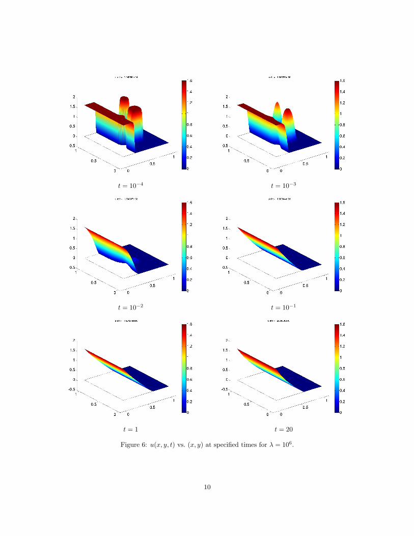
case. All of these images were created using a 128× 128 mesh of linear Lagrange elements.Specifically, we discuss the results for λ = 106 in Figures 6, 7, 8, and 9 in detail now. Figures 6, 7, and 8

show the evolution over time of the chemical species u, v, and w, respectively for λ = 106. For example, wesee in Figure 6 that over time, u starts from the initial condition in Figure 1 with u = α = 1.6 along x = 0and u = 0 along x = 1. Over a short period of time in the first frame of Figure 6, the sharp edges, whichrepresent a sharp drop off in the amount of chemical, has rounded off as some of the chemical towards theedge reacts with some of the other chemical. As time progresses, we see that the mound has rounded offeven more. In the next frame, the mounds have almost completely disappeared. In the last two frames, thechemical has just about settled into its steady state. There is a similar progression in the v images in Figure 7,with v = 0 along x = 0 and v = β = 0.8 along x = 1. In the w images in Figure 8, we see that the simulationstarts with w = 0 throughout Ω in Figure 1 and that some w > 0 develops first along the reaction interfacesin the first frame of Figure 8. As time progresses in the next few frames, we see that the areas with less wstart to fill in by diffusion from the reaction interface, which is the only place where w is generated. In thefollowing two frames, the peak amount of w still follows the reaction interface. But eventually, the amountof w is highest in the right portion of the domain; this results from the fact that the intermediate species isconsumed in a reaction with the first species u, but not the second v, hence it can diffuse from the reaction

4

interface to the right without consumption, while the concentration of w progressively decreases as it diffusesfrom the reaction interface to the left of the interface. We observe that the growth of w slows down overtime towards an apparently finite steady state value; that is a significant observation, for which a rigorousproof is only being developed at present [5]. The most interesting set of images is the collection of interfaceimages in Figure 9. We see here the outlines of the actual reaction interface where u > 0 and v > 0 meetby diffusion and react rapidly with rate λuv. Recall that at the initial time, these two species do not coexistand mathematically uv = 0. It is only by diffusion that positive values of both get in contact with each otherand this gives the first positive values of the resulting reaction intermediate w. Numerically, we determinethe location of the interface as a contour plot with one contour level of value 0 of the difference u− v. In thefirst frame of Figure 9 at t = 10−4, we can still clearly see the ‘head’ connected by the ‘neck’ to the ‘body’on the left portion of the domain and an disjoint ‘disk’ in the upper right of the domain, like in the initialcondition in Figure 1; these outlines have the same shape as the locations of w > 0 at the corresponding timein Figure 8. In the next frame, we see the head separating from the body in the left portion of the domain,before it re-attaches to the body in the following frame. Also by the time of the third frame, the disjointeddisk has vanished with its supply of the u species completely consumed. The chosen initial conditions giverise to an interesting behavior in that the head separates and then re-attaches to the body in the left portionof the domain, while at the same time the disk disappears. In the last three frames, we see the interface tendsto its steady state location at x∗ ≈ 0.6.

Comparing the set of figures for λ = 106 to the corresponding ones for the other values of λ as well as thetwo component model with λ =∞ in Figures 14, 15, 16, and 17, we can clearly see that the progression overtime is essentially identical up to the graphical resolution of the studies.

3.2 Accuracy and Efficiency Comparisons

The graphical results in the figures in the previous section indicate that the two component model appears togive results that are qualitatively consistent with the three species model in the asymptotic limit of λ → ∞.This section defines four measures to study the accuracy of the two component model quantitatively. As ourgoal in this report is to verify that the two component model is numerically superior to the three speciesmodel, we also define two measures to validate the efficiency quantitatively. The four measures of accuracyand two measures of efficiency are studied over a variety of finite element meshes with N ×N elements.

The first measure of accuracy is the closeness of the location x∗ of the interface at the final time of thetransient problem to that of the actual steady state interface, which is x∗steady = 0.601806640625; this valuewas obtained by simulations of the three species steady state problem in 1-D on a high resolution mesh withN = 8,192 and will be considered the true value for x∗ in the following. The other measures of accuracy arethree times t1, t2, and t3 defined by significant transitions in the development of the interface plot. The time t1represents the time at which the head separates from the body in the left portion of the domain; t2 representsthe time at which the head re-attaches to the body, and t3 represents the time at which the disjoint disk inthe upper right of the domain dissipates. These times were obtained by viewing movies of the interface, wherethe movies were compiled using the output of all time steps from the ODE solver, which are substantiallymore than the six times in the figures. Thus the times listed are as precise as possible for each simulation, butare limited in accuracy by the number of time steps and their exact choice made by the time step selectionalgorithm in the ODE solver. The x∗ values in Table 1 are identical for the λ = 106, 109, and ∞ cases. Theyare slightly different among the mesh resolutions, but within the mesh resolution to x∗steady in each case. Inλ = 103 case, the x∗ values are slightly off, because they have not reached their asymptotic values, yet. Wesee in Table 1 that the corresponding times t1, t2, and t3 are very close for all λ = 103, 106, 109, and ∞, foreach fixed mesh resolution N ×N . The difference in the values of the times between different mesh resolutionsis explained by the fact that they generate slightly different initial conditions, depending on how exactly thecurved boundaries in the initial conditions are resolved, which result in slightly different behavior over time.Because the accuracy results are nearly identical across at least λ = 106, 109, and ∞ for each fixed meshresolution, these accuracy measures confirm that the two component model (λ =∞) is an accurate simulatorfor the three species model in the asymptotic limit.

As measures of efficiency, we consider the number of time steps taken by the ODE solver and the total

5

t = 10−4 t = 10−3

t = 10−2 t = 10−1

t = 1 t = 20

Figure 2: u(x, y, t) vs. (x, y) at specified times for λ = 103.

6

t = 10−4 t = 10−3

t = 10−2 t = 10−1

t = 1 t = 20

Figure 3: v(x, y, t) vs. (x, y) at specified times for λ = 103.

7

t = 10−4 t = 10−3

t = 10−2 t = 10−1

t = 1 t = 20

Figure 4: w(x, y, t) vs. (x, y) at specified times for λ = 103.

8

t = 10−4 t = 10−3

t = 10−2 t = 10−1

t = 1 t = 20

Figure 5: Interface at specified times for λ = 103.

9

t = 10−4 t = 10−3

t = 10−2 t = 10−1

t = 1 t = 20

Figure 6: u(x, y, t) vs. (x, y) at specified times for λ = 106.

10

t = 10−4 t = 10−3

t = 10−2 t = 10−1

t = 1 t = 20

Figure 7: v(x, y, t) vs. (x, y) at specified times for λ = 106.

11

t = 10−4 t = 10−3

t = 10−2 t = 10−1

t = 1 t = 20

Figure 8: w(x, y, t) vs. (x, y) at specified times for λ = 106.

12

t = 10−4 t = 10−3

t = 10−2 t = 10−1

t = 1 t = 20

Figure 9: Interface at specified times for λ = 106.

13

t = 10−4 t = 10−3

t = 10−2 t = 10−1

t = 1 t = 20

Figure 10: u(x, y, t) vs. (x, y) at specified times for λ = 109.

14

t = 10−4 t = 10−3

t = 10−2 t = 10−1

t = 1 t = 20

Figure 11: v(x, y, t) vs. (x, y) at specified times for λ = 109.

15

t = 10−4 t = 10−3

t = 10−2 t = 10−1

t = 1 t = 20

Figure 12: w(x, y, t) vs. (x, y) at specified times for λ = 109.

16

t = 10−4 t = 10−3

t = 10−2 t = 10−1

t = 1 t = 20

Figure 13: Interface at specified times for λ = 109.

17

t = 10−4 t = 10−3

t = 10−2 t = 10−1

t = 1 t = 20

Figure 14: u(x, y, t) vs. (x, y) at specified times for λ =∞.

18

t = 10−4 t = 10−3

t = 10−2 t = 10−1

t = 1 t = 20

Figure 15: v(x, y, t) vs. (x, y) at specified times for λ =∞.

19

t = 10−4 t = 10−3

t = 10−2 t = 10−1

t = 1 t = 20

Figure 16: w(x, y, t) vs. (x, y) at specified times for λ =∞.

20

t = 10−4 t = 10−3

t = 10−2 t = 10−1

t = 1 t = 20

Figure 17: Interface at specified times for λ =∞.

21

Table 1: Summary of accuracy and efficiency data for simulations of the three species model with λ = 103,106, and 109, and the two component model with λ =∞.

λ = 103

Resolution Time to Complete (s) Time Steps x∗ t1(×10−4) t2(×10−3) t3(×10−3)64× 64 43 215 0.609375000 1.608304 7.077499 7.077499

128× 128 166 230 0.609375000 4.961102 6.354030 6.768004256× 256 771 249 0.601562500 3.716557 6.972642 6.972642

λ = 106

Resolution Time to Complete (s) Time Steps x∗ t1(×10−4) t2(×10−3) t3(×10−3)64× 64 140 573 0.625000000 1.567014 6.863272 6.795620

128× 128 467 571 0.609375000 4.831523 6.317239 6.768036256× 256 2,463 548 0.605468750 3.578299 6.753300 6.836752

λ = 109

Resolution Time to Complete (s) Time Steps x∗ t1(×10−4) t2(×10−3) t3(×10−3)64× 64 231 646 0.625000000 1.661473 6.862192 6.790343

128× 128 1,802 1,743 0.609375000 4.804291 6.267175 6.696524256× 256 11,391 2,353 0.605468750 3.612976 6.685775 6.791933

λ =∞Resolution Time to Complete (s) Time Steps x∗ t1(×10−4) t2(×10−3) t3(×10−3)

64× 64 31 203 0.625000000 1.564306 6.903623 6.903623128× 128 95 229 0.609375000 4.910450 6.459946 6.623560256× 256 444 234 0.605468750 3.619295 7.091791 7.091791

computation time in seconds taken by the COMSOL script. We see from Table 1 that the number of timesteps for each λ value is on the same order of magnitude for all N ×N meshes reported, except for the mostnumerically challenging λ = 109 case. The computation times get significantly larger for the finer meshes dueto the larger linear systems that need to be solved in each time step. For each fixed N , as λ increases, the timeof computation and the number of time steps increase rapidly for the finite λ values. But for two componentmodel with λ = ∞ in Table 1, the number of time steps are again on the scale of the λ = 103 case. Thisindicates that the smoothness of the two component model is comparable to the three species model with thismoderate λ value; the computation time is even faster than that case resulting from the smaller number ofunknowns in the system for two PDEs in the two component model as compared to three for the three speciesmodel. We point out that in the case of the 64 × 64 mesh for λ = 109, the ODE solver failed to converge atthe ODE tolerances stated above and used for all other cases. However, this was for a different reason thanwith the original ODE solver. The original solver failed to find suitable convergence for initial conditions,while in this case the solver computed until it hit a point in time where it could not compute further giventhe minimum time step value. Thus the data listed in the table is computed with relative and absolute ODEtolerences that are one order of magnitude coarser than the ones used for all other cases.

Taken together, because the accuracy results are nearly identical across at least λ = 106, 109, and ∞ foreach fixed mesh resolution, the accuracy and efficiency measures demonstrate that the two component model(λ =∞) is an accurate and efficient simulator for the three species model in the asymptotic limit on a givenmesh.

22

Acknowledgments

The hardware used in the computational studies is part of the UMBC High Performance Computing Facility(HPCF). The facility is supported by the U.S. National Science Foundation through the MRI program (grantno. CNS–0821258) and the SCREMS program (grant no. DMS–0821311), with additional substantial supportfrom the University of Maryland, Baltimore County (UMBC). See www.umbc.edu/hpcf for more informationon HPCF and the projects using its resources.

References

[1] Leonid V. Kalachev and Thomas I. Seidman. Singular perturbation analysis of a stationary diffu-sion/reaction system whose solution exhibits a corner-type behavior in the interior of the domain. J.Math. Anal. Appl., vol. 288, pp. 722–743, 2003.

[2] Michael Muscedere and Matthias K. Gobbert. Parameter study of a reaction-diffusion system near thereactant coefficient asymptotic limit. Dynamics of Continuous, Discrete and Impulsive Systems Series ASupplement, pp. 29–36, 2009.

[3] Thomas I. Seidman. Interface conditions for a singular reaction-diffusion system. Discrete and Cont.Dynamical Systems, to appear.

[4] Thomas I. Seidman and Leonid V. Kalachev. A one-dimensional reaction/diffusion system with a fastreaction. J. Math. Anal. Appl., vol. 209, pp. 392–414, 1997.

[5] Thomas I. Seidman and Adrian Muntean. Fast-reaction asymptotics for a time-dependent reaction-diffusionsystem with a nonlinear source term. In preparation.

[6] Ana Maria Soane, Matthias K. Gobbert, and Thomas I. Seidman. Numerical exploration of a system ofreaction-diffusion equations with internal and transient layers. Nonlinear Anal.: Real World Appl., vol. 6,no. 5, pp. 914–934, 2005.

[7] Guan Wang, Aaron Churchill, Matthias K. Gobbert, and Thomas I. Seidman. Efficient computationfor a reaction-diffusion system with a fast reaction with continuous and discontinuous initial data usingCOMSOL Multiphysics. Technical Report HPCF–2009–3, UMBC High Performance Computing Facility,University of Maryland, Baltimore County, 2009.

23