Solving a reaction-diffusion system with chemotaxis and

non-local terms using Generalized Finite Difference

Method. Study of the convergence

J.J. Benitoa,1, A. Garcıaa, L. Gaveteb, M. Negreanuc, F. Urenaa,∗, A.M.Vargasc

aUNED, ETSII, Madrid, Spainb UPM, ETSIM, Madrid, Spain

cInstituto de Matematica Interdisciplinar, Depto. de Analisis Matematico y MatematicaAplicada, UCM, Madrid, Spain

Abstract

In this paper a parabolic-parabolic chemotaxis system of PDEs that describesthe evolution of a population with non-local terms is studied. We derive thediscretization of the system using the meshless method called Generalized Fi-nite Difference Method. We prove the conditional convergence of the solutionobtained from the numerical method to the analytical solution in the two-dimensional case. Several examples of the application are given to illustratethe accuracy and efficiency of the numerical method. We also present two ex-amples of a parabolic-elliptic model, as generalized by the parabolic-parabolicsystem addressed in this paper, to show the validity of the discretization ofthe non-local terms.

Keywords: Chemotaxis system, Generalized Finite Difference, Meshlessmethod, Asymptotic stability.

1. Introduction

Chemotaxis is the process under which some living organisms (such asbacterias, cells of the immune system, cells of the endothelium, etc.) direct

∗Corresponding authorEmail addresses: jbenito@ind.uned.es (J.J. Benito), angelochurri@gmail.com

(A. Garcıa), lu.gavete@upm.es (L. Gavete), negreanu@mat.ucm.es (M. Negreanu),furenaprieto@gmail.com (F. Urena), antonvar@ucm.es (A.M. Vargas)

Preprint submitted to Journal of Computational and Applied MathematicsDecember 15, 2020

its movement in the direction of a chemical gradient. The individuals of thebiological species are able to recognize the chemical signal, to measure its con-centration and to move towards the higher concentrations of the substance(positive taxis) or away from it (negative taxis). Mathematical models withchemotactic terms have been applied to model Angiogenesis, a key process inTumor Growth (see for instance Anderson and Chaplain [1]), in Astrophysicsto describe gravitational interaction of particles on the gravitational equilib-rium of polytropic stars; in ecology, to describe the attraction of predatorsto certain chemical signals (pheromons) of the prey in morphogenesis, thecreation of shapes and organs in embryonic development, etc.Since 1970s, chemotaxis has been studied from a mathematical point ofview, starting with the first models of PDEs suggested by Keller and Segel[5]. Mathematical bibliography concerning this phenomenon is extensive, al-though many important results obtained in the area during the last decadescan be found in Horstmann [4].In this paper we consider a parabolic-parabolic system of quasilinear PDEsdescribing the interactions between the population’s density of a biologicalspecies, “U”, and the chemical substance, “V ”, responsible for the chemo-tactic process:

∂U

∂t= ∆U − χdiv(Um∇V ) + U

(a0 − a1U

α + a2

∫Ω

Uαdx

), Ω× (0,∞),

d∂V

∂t= ∆V − V + Uγ, Ω× (0,∞),

U(x, 0) = U0(x), V (x, 0) = V0(x) x ∈ Ω,

∂U

∂ν=∂V

∂ν= 0 ∂Ω× (0,∞).

(1)All the theoretical results of the manuscript are given for the case d 6= 0, inparticular, without loss of generality, we consider throughout the text d=1.For d = 0, we present in examples 5 and 6 the behavior of the solution,though the proof of the main result of the paper is devoted to the case d = 1.Model (1) is a generalization of the one considered in [3] where can be founda wide summary of the main results related to (ref1) in the particular casea2 = 0, i.e., the global existence of the solutions and the asymptotic stabilityof the point ((a0/a1)1/α, (a0/a1)γ/α), with a1 large enough, are done.The coefficient “a0”, sometimes also called Malthusian parameter, inducesan exponential growth for low density populations if a0 > 0. If a1 > 0, the

2

mechanism that limits the growth of biological species U is given by the term−a1U

α and it generalizes the most frequent case α = 1. At the time thatthe population grows, the competitive effect of the local term a1U

α becomesmore influential. We also consider a non-local term in the logistic source asa2

∫ΩUα describing the effects of the total mass of the species in the growth

of the population. If a2 < 0 there is competition among the individuals ofthe species for the resources and if a2 > 0, individuals cooperate globallyto survive although they compete locally. In the last case, the individualscompete locally but cooperate globally and the effects of a1U

α and a2

∫ΩUα

balance the system. Non-local terms of such kind have already been used.For instance, in [9] integral terms were used to describe the competition be-tween the cancer cell density and the extracellular matrix density. Also, in [6]authors considered a parabolic-elliptic PDE system with non-local terms andthey obtained the global existence of the solutions together with its asymp-totic behavior whenever a1 > 2χ+ |a2|.The non-linear nature of the chemotaxis term has been studied in the liter-ature by different authors, see [4] and references therein. The exponent mindicates nonlinearities with respect to U in the tactic sensitivity functions;intuitively, there is a reinforcement of movement in direction of ∇V wherethe population U is greater than a normalized value and presents a weakermovement where it is less than it. These terms with α ≥ 1 induce a neg-ative feedback that slows growth as populations approach their maximumsize and a stronger intra-specific concurrence, (via exponents of the involveddensity).Due to its importance in applied sciences as Biology, Chemical Engineer-ing and Medicine, and the inherent complexity of the system, because of thenon-linearity and non-locality, it is necessary to develop numerical algorithmswhich are able to solve efficiently system (1).In this paper we propose the Generalized Finite Difference Method (GFDM).This meshless method has been recently proved to solve with accuracy highlynonlinear PDEs, see [10, 11]. In [2], the authors obtained conditional con-vergence for the parabolic-elliptic case of system (1) for d = a2 = 0, a0 = a1

and m = α = γ = 1. In the cited paper, the conditional convergence of thenumerical method is proved in a very different way than in the present pa-per. Due to the nature of the system, we were able to substitute the terms ofthe elliptic equation into the parabolic one, which simplified the test. In thepresent paper we shall use matrix arguments. The differences between theparabolic-elliptic system and the parabolic-parabolic one are also significant

3

in the analytical proof of the continuous models, as can be seen in [7] and [8].Furthermore, the novelty of this paper is the introduction and discretizationof non-local terms, which is a challenging task and a problem of growinginterest.The paper is organized as follows: in Section 2 we present some preliminariesof the GFD method, which can be found in [10, 11] and the references therein,although for completeness, we mention them below. Section 3 is devoted tothe proof of Theorem 3.1, where we find the conditions on the time step of theGFD explicit scheme under which it is convergent. In Section 4 we find theconstant steady states of system (1) and present several numerical examplesto illustrate its asymptotic stability. In addition, we present some examplesof a parabolic-elliptic model to show the validity of the discretization of thenon-local terms. We finally present some conclusions.

2. Preliminaries

Consider a domain Ω ⊂ R2 and let be M = x1, . . . ,xN ⊂ Ω a discretiza-tion of it with N points. For each x0 ∈M , we define Es = x0;x1, . . . ,xs ⊂M , where xi (i = 1, . . . , s) can be chosen in several ways, by different criteria.We call xi = (xi, yi) and we denote by hi := xi − x0 and ki := yi − y0. Letbe F ∈ C4(Ω). Since no confusion with the initial data of F is possible, wewrite in this section F0 = F (x0) = F (x0, y0) and Fi = F (xi). By Taylorseries expansion, for i = 1, ..., s, we have :

Fi = F0 + hi∂F0

∂x+ ki

∂F0

∂y+

1

2

(h2i

∂2F0

∂x2+ k2

i

∂2F0

∂y2+ 2hiki

∂2F0

∂x∂y

)+ ... (2)

By ignoring the third and higher order terms in (2), we obtain a second orderapproximation fi of F in xi. Moreover, we take the vector

D5 =

∂f0

∂x,∂f0

∂y,∂2f0

∂x2,∂2f0

∂y2,∂2f0

∂x∂y

. (3)

In this way, we can obtain an approximation of function Fi in terms of thecoefficients of D5. In order to determine these, we minimize with respect tothe partial derivatives the following function

B(f) =s∑i=1

[(f0 − fi) + hi∂f0

∂x+ ki

∂f0

∂y+

+1

2(h2

i

∂2f0

∂x2+ k2

i

∂2f0

∂y2+ 2hiki

∂2f0

∂x∂y)]2w2

i

(4)

4

where wi = w(hi, ki) are positive symmetrical monotone decreasing weightingfunctions. One arrives then to the following system of linear equations

A(hi, ki, wi)DT5 = b(hi, ki, wi, u0, ui), (5)

where

A =

h1 h2 · · · hsk1 k2 · · · ks...

......

...h1k1 h2k2 · · · hsks

ω21

ω22

· · ·ω2s

h1 k1 · · · h1k1

h2 k2 · · · h2k2...

......

...hs ks · · · hsks

.

Some assumptions on the selection criteria of the nodes of Es must be madein order to guarantee that A is positive definite (see [10, 11] for more detailson the selection criteria and the weighting functions). By solving system (5),we can find the discretization of the spatial derivatives as functions of f0 andfi:

∂f(x0, n∆t)

∂x= −m01f

n0 +

s∑i=1

mi1fni +O(h2

i , k2i ), with m01 =

s∑i=1

mi1,

∂f(x0, n∆t)

∂y= −m02f

n0 +

s∑i=1

mi2fni +O(h2

i , k2i ), with m02 =

s∑i=1

mi2,

∂2f(x0, n∆t)

∂x2= −m03f

n0 +

s∑i=1

mi3fni +O(h2

i , k2i ), with m03 =

s∑i=1

mi3,

∂2f(x0, n∆t)

∂y2= −m04f

n0 +

s∑i=1

mi4fni +O(h2

i , k2i ), with m04 =

s∑i=1

mi4,

∂2f(x0, n∆t)

∂x∂y= −m05f

n0 +

s∑i=1

mi5fni +O(h2

i , k2i ), with m05 =

s∑i=1

mi5.

(6)

Remark 2.1. For simplicity, for the discretization of the laplacian operator,we write

∆f(x0, n∆t) = −m00fn0 +

s∑i=1

mi0fni ,

where m00 = m03 +m04 and mi0 = mi3 +mi4.

5

The time derivative is approximated by

∂f(x0, y0, n∆t)

∂t=fn+1

0 − fn0∆t

+O(∆t). (7)

Finally, the nonlocal term can be expressed by means of the Taylor seriesexpansion as∫

Ω

F (x+ x0, y + y0)dx =

∫Ω

(F (x0) + x

∂F

∂x(x0) + y

∂F

∂y(x0)

+x2

2

∂2F

∂x2(x0) + xy

∂2F

∂x∂y(x0) +

y2

2

∂2F

∂y2(x0) +R2

)dx,

(8)

where R2 is such that

lim(x,y)→(0,0)

R2

‖(x, y)‖2= 0.

In order to prove the main result of the paper concerning the conditionalconvergence of the GFD scheme for solving system (1) we need the followingbasic results.

Lemma 2.1. Let M ∈ Mn×n(R). If there exists some matrix norm suchthat ‖M‖ < 1, then

limk→∞

Mk = 0.

Lemma 2.2. Assume M ∈ Mn×n(R), then the following statements areequivalent

i. limk→∞Mk = 0,

ii. ρ(M) < 1,

where ρ(·) stands for the spectral radius.

6

3. GFDM explicit scheme

Using the approximations given by (6), (7) and (8), we obtain the follow-ing 2-dimensional GFD explicit scheme:

un+10 =un0 + ∆t

[−m00u

n0 +

s∑i=1

mi0uni − χ(un0 )m

(−m00v

n0 +

s∑i=1

mi0vni

)]

− χ(un0 )m−1∆t

(−m01u

n0 +

s∑i=1

+mi1uni

)(−m01v

n0 +

s∑i=1

mi1vni

)

− χ(un0 )m−1∆t

(−m02u

n0 +

s∑i=1

+mi2uni

)(−m02v

n0 +

s∑i=1

mi2vni

)

+ ∆tun0

[a0 − a1(un0 )α + a2

((un0 )α +

α

2(un0 )α−1

(−(m01 +m02)un0

+s∑i=1

(mi1 +mi2)uni

)+α(α− 1)

6(un0 )α−2

(−m00u

n0 +

s∑i=1

mi0uni

)

+α(α− 1)

4(un0 )α−2

(−m05u

n0 +

s∑i=1

mi5uni

))]+O(h2

i , k2i )

vn+10 =−m00v

n0 +

s∑i=1

mi0vn0 − vn0 + (un0 )γ +O(∆t(h2

i , k2i )).

(9)

Remark 3.1. From now, unless otherwise stated, d = 1. Note that equation(9) holds since Ω = [0, 1]× [0, 1]. In other case the coefficients resulting from(8) may vary although the following theorem remains true. For an arbitraryand irregular domain we shall make∫

Ω

F (x+ x0, y + y0)dx = F (x0) +∂F

∂x(x0)

∫Ω

xdx +∂F

∂y(x0)

∫Ω

ydx

+∂2F

∂x2(x0)

∫Ω

x2

2dx +

∂2F

∂x∂y(x0)

∫Ω

xydx +∂2F

∂y2(x0)

∫Ω

y2

2dx +R2,

(10)

and use numerical integration and interpolation if necessary to obtain thevalue of the integrals appearing in (10). The inclusion of such values in thenumerical scheme (9) is a straightforward computation.

7

The following result proves that the explicit scheme given by (9) is condi-tionally convergent for the fully parabolic case.

Theorem 3.1. Let (U, V ) be the exact solution of (1). Let a0, a1 > 0,a2 ∈ R, d = 1 and m,α, γ ≥ 1. Then, the GFD explicit scheme (9) isconvergent if

∆t <2

m00 +∑s

i=1 |mi0|+ |Φ|+ |Ψ|, (11)

8

where

Φ : = −χm(m− 1)((m01)2 + (m02)2)ξm−21

+ χm(m− 1)ξm−22 m01v

n0

s∑i=1

mi1uni + χm2ξm−1

3 m01

s∑i=1

mi1vni

− χm(m− 1)ξm−24

(s∑i=1

mi1uni

)(s∑i=1

mi1vni

)+ χm(m− 1)ξm−2

5 m05vn0

s∑i=1

mi2uni

+ χm2ξm−16 m02

s∑i=1

mi2vni − χm(m− 1)ξm−2

7

(s∑i=1

mi2uni

)(s∑i=1

mi2vni

)

χmξm−18 m00v

n0 − χmξm−1

9

s∑i=1

mi0vni + a0 − (a1 − a2)(α + 1)ξα10

− a2α(α + 1)ξα11

2(m01 +m02) +

a2α2ξα−1

12

2

s∑i=1

(mi1 +mi2)uni

− a2α2(α− 1)ξα−1

13

6m00 +

a2α(α− 1)2ξα−214

6

s∑i=1

mi0uni

− a2α2(α− 1)ξα−2

15

4m05 +

a2α(α− 1)2ξα−116

4

s∑i=1

mi5uni

+ |χm(Un0 )m−1vn0m01

s∑i=1

mi1|+ |χm(Un0 )m−1

s∑i=1

mi1vni |

s∑i=1

|mi1|

+ |χm(Un0 )m−1vn0m02

s∑i=1

mi2|+ |χm(Un0 )m−1

s∑i=1

mi2vni |

s∑i=1

|mi2|

|a2|α2

(Un0 )α

s∑i=1

|mi1 +mi2|+

∣∣∣∣∣a2α(α− 1)(Un0 )α−1

6

∣∣∣∣∣s∑i=1

|mi0|

+

∣∣∣∣∣a2α(α− 1)(Un0 )α−1

4

∣∣∣∣∣s∑i=1

|mi5|,

(12)

9

and

|Ψ| :=

∣∣∣∣∣−χm(Un0 )m[(m01)2 + (m02)2] + χm(Un

0 )m−1m01

s∑i=1

mi1Uni

+ χm(Un0 )m−1m02

s∑i=1

mi2Uni − χ(Un

0 )mm00

∣∣∣∣∣+ |χm(Un

0 )mm01|s∑i=1

|mi1|+ |χm(Un0 )m−1

s∑i=1

mi1Uni |

s∑i=1

|mi1|

+ |χm(Un0 )mm02|

s∑i=1

|mi2|+ |χm(Un0 )m−1

s∑i=1

mi2Uni |

s∑i=1

|mi2|

+ |χ(Un0 )m|

s∑i=1

|mi0|,

(13)

for some ξj ∈ (uni , Uni ) ∩ (Un

i , uni ), ∀j ∈ 1, ..., 16,∀i ∈ 0, 1, ..., s.

Proof. Consider the first equation of (9) (approximate solution) and sub-tract the same expression for the exact solution, i.e., in terms of Un

i and V ni

(which stands for the exact solution at time n∆t). Let us call uni := uni −Uni

(similarly for vni ) and take the maximum of uni among all nodes of the star,that is, un := maxi=0,...,s |uni |. Then, after some straightforward computations(the reader may see [2] for further details of the computations) together withthe Mean Value Theorem applied to the functions

f(λ) = (λ)δ, δ = m,α,

we arrive to the following

un+1 ≤ un

[|1−∆tm00|+ ∆t

∑i=1

|mi0|+ ∆t|Φ|

]+ ∆t|Ψ|vn, (14)

where Φ and Ψ are defined in (12) and (13), respectively. If we perform thesame computations with the second equation of (9) and its expression for theexact solution, it yields

vn0 − vn0∆t

= −(m00 + 1)vn0 +s∑i=1

mi0vni + γξγ−1

17 un0 . (15)

10

Again, by taking bounds and rewritting (15) in terms of un, vn, we get

vn+1 ≤ un∆tγξγ−117 + vn[|1−∆t(m00 + 1)|+ ∆t

s∑i=1

|mi0|]. (16)

Therefore, inequalities (14) and (16) can be expressed as(un+1

vn+1

)≤(M11 M12

M21 M22

)(un

vn

)(17)

for an obvious choice of Mlr, with r, l ∈ 1, 2. Convergence of the explicitscheme is assured if the eigenvalues of (Mrl) are all smaller than 1. Considerthe ‖ · ‖1 norm as the maximum sum by rows. Clearly, since ∆t << 1,‖M‖1 = M11 +M12 and, by assuming,

∆t <2

m00 +∑s

i=1 |mi0|+ |Φ|+ |Ψ|, (18)

we have that ‖M‖1 < 1. Therefore, Lemma 2.1 implies limk→∞Mk = 0.

Finally, by Lemma 2.2 we obtain that the spectral radius is less that 1,which proves the result.

Remark 3.2. The above result covers only the parabolic-parabolic case withd 6= 0. The conditional convergence of the GFD explicit scheme for theparabolic-elliptic case, i.e., d = 0, has been obtained in [2] by the authors.

4. Numerical examples

In this section we present numerical examples of the applicability of theGFD scheme given by (9) for solving the non-linear non-local system (1). Forour simulations we use as time step ∆t = 0.001 and consider as discretizationof the domain Ω = [0, 1]× [0, 1] both regular and irregular clouds of points ofFigure 1, each one with 437 nodes. We have chosen the potential weightingfunction w = 1

dist4and performed our simulations using an 8-node star in all

cases.Notice that we have introduced some ficticious or vitual nodes (black nodesin Figure 1) in order to deal with the homogeneous Neumann boundaryconditions,

∂U

∂ν=∂V

∂ν= 0,

11

Figure 1: Regular and irregular clouds of points

since we use the central difference, which is of second order, if the domainΩ has regular boundary (in the sense of the distribution of nodes) and GFDformulae in other case. For all examples we compute the difference betweenthe numerical solution and the constant steady states using the l∞ norm,that is,

‖v‖l∞(Ω) = maxi=0,...,N

|vi|.

In order to illustrate the accuracy of this meshless method, let us firstfind the steady states of the problem.

4.1. Steady states

In order to study the asymptotic behavior of system (1) we look at theconstant steady states (u∗, v∗). We assume, without loss of generality, that|Ω| = 1.

Lemma 4.1. Assume a0, a1, α, γ > 0, a1 > |a2| then the constant steadystate of (1) is

(u∗, v∗) =

(α

√a0

a1 − a2

,

(α

√a0

a1 − a2

)γ). (19)

Proof. Steady states of system (1) are the solutions to the homogeneousone 0 = a0 − a1(u∗)α + a2

∫Ω

(u∗)αdx,

0 = −v∗ + (u∗)γ.

(20)

12

T(s) 0 2.5 5 7.5 10

‖√

22− u‖l∞(Ω) 1.2929 0.0024 0.0001 0e-03 0e-04

‖0.5− v‖l∞(Ω) 0.5000 0.0436 0.0036 0.2929e-03 0.2401e-4

Table 1: Values of ‖√

22 − u‖l∞(Ω) and ‖0.5− v‖l∞(Ω) in the Example 1.

Since |Ω| = 1, the first equation lead us to

(u∗)α =a0

a1 − a2

,

and by the second equation we arrive to the result for v∗.

Remark 4.1. The above result covers the following two particular cases:

1. Clearly, if we make α = m = γ = 1 and d = 0, the result is the oneobtained by Negreanu and Tello [6].

2. Also, by making d = 1, a0 = r, a1 = µ and a2 = 0, Ding et al [3]obtained the convergence of the solution to the constant steady state(u∗, v∗).

Asymptotic stability of the steady state has been obtained in both papers.

Remark 4.2. If a0, a2 ≤ 0, for any a1 > 0, the solution converges asymp-totically to 0, again in accordance with [3].

4.2. Example 1

In this first example we solve the case which appears in [3], that is to say,the case of Remark 4.1. Therefore we fix a2 = 0. Consider U0(x, y) = 2x2

and V0(x, y) = exp(−10[(x−1.2)2 +(y−1)2]). Assume the following relationof parameters: d = 1, m = 1, α = 2, γ = 2, χ = 0.5 and a0 = 2, a1 = 4.Then, by theory, we expect to find convergence towards (

√2

2, 1

2). We consider

the regular cloud of points of Figure 1.

Table 1 shows the values of the l∞ norm of the difference of the solutionand the asymptotic value at different times, and Figure 2 the discrete solutionat 0, 2.5 and 10 seconds.

13

Figure 2: u, v-solution for 0, 2.5 and 10 seconds in the Example 1.

4.3. Example 2

We now consider a0 = a2 = −1 and a1 = 1 for initial data U0(x, y) =exp(−10[(x−0.5)2 + (y−0.5)2]) and V0(x, y) = 0.5 exp(−10[(x−0.2)2 + (y−1)2]) in the irregular cloud of points. Also we put d = 1, m = 1, α = 2, γ = 1and χ = 0.5. As stated in Remark 4.2 we expect to find asymptotic decay ofthe solution to 0.

Table 2 presents the l∞ norm of the numerical solution at times 0, 2.5,5, 7.5 and 10 seconds and Figure 3 the plot of the solution at 0, 2.5 and 10seconds. As stated, solution tends to zero very rapidly.

4.4. Example 3

Consider as initial data U0(x, y) = exp(−10[(x− 0.1)2 + (y − 0.1)2]) andV0(x, y) = 0.7 exp(−10[(x − 1.2)2 + (y − 1)2]). We choose the relation of

14

T(s) 0 2.5 5 7.5 10‖u‖l∞(Ω) 0.9990 0.0234 0.0019 0.0002 0.0129e-03‖v‖l∞(Ω) 0.4975 0.0639 0.0100 0.0012 0.1321e-03

Table 2: Values of ‖u‖l∞(Ω) and ‖v‖l∞(Ω) in the Example 2.

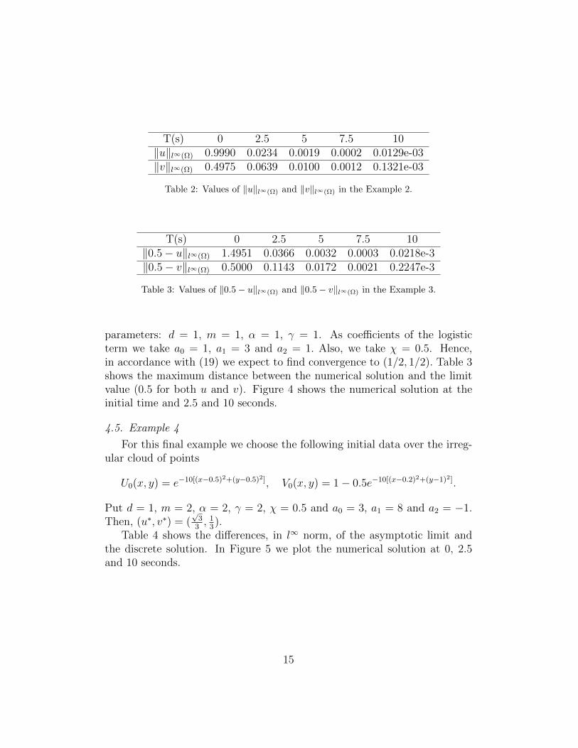
T(s) 0 2.5 5 7.5 10‖0.5− u‖l∞(Ω) 1.4951 0.0366 0.0032 0.0003 0.0218e-3‖0.5− v‖l∞(Ω) 0.5000 0.1143 0.0172 0.0021 0.2247e-3

Table 3: Values of ‖0.5− u‖l∞(Ω) and ‖0.5− v‖l∞(Ω) in the Example 3.

parameters: d = 1, m = 1, α = 1, γ = 1. As coefficients of the logisticterm we take a0 = 1, a1 = 3 and a2 = 1. Also, we take χ = 0.5. Hence,in accordance with (19) we expect to find convergence to (1/2, 1/2). Table 3shows the maximum distance between the numerical solution and the limitvalue (0.5 for both u and v). Figure 4 shows the numerical solution at theinitial time and 2.5 and 10 seconds.

4.5. Example 4

For this final example we choose the following initial data over the irreg-ular cloud of points

U0(x, y) = e−10[(x−0.5)2+(y−0.5)2], V0(x, y) = 1− 0.5e−10[(x−0.2)2+(y−1)2].

Put d = 1, m = 2, α = 2, γ = 2, χ = 0.5 and a0 = 3, a1 = 8 and a2 = −1.Then, (u∗, v∗) = (

√3

3, 1

3).

Table 4 shows the differences, in l∞ norm, of the asymptotic limit andthe discrete solution. In Figure 5 we plot the numerical solution at 0, 2.5and 10 seconds.

15

Figure 3: u, v-solution for 0, 2.5 and 10 seconds in the Example 2.

T(s) 0 2.5 5 7.5 10

‖√

33− u‖l∞(Ω) 0.5774 0.0003 0.0000 0e-03 0e-04

‖13− v‖l∞(Ω) 0.6667 0.0419 0.0034 0.2815e-03 0.2308e-4

Table 4: Values of ‖√

33 − u‖l∞(Ω) and ‖ 1

3 − v‖l∞(Ω) in the Example 4.

16

Figure 4: u, v-solution for 0, 2.5 and 10 seconds in the Example 3.

17

Figure 5: u, v-solution for 0, 2.5 and 10 seconds in the Example 4.

18

T(s) 0 2.5 5 7.5 10‖1

4− u‖l∞(Ω) 0.75 0.0141 0.0011 8.9589e-05 7.3423e-06

‖14− v‖l∞(Ω) - 0.0141 0.0011 8.9679e-05 7.3497e-06

Table 5: Values of ‖ 14 − u‖l∞(Ω) and ‖ 1

4 − v‖l∞(Ω) in the Example 5.

4.6. Example 5

In this example we consider the parabolic-elliptic system (0.1) of [6] withf = 0, d = 0 and λ = 1 (also m = α = γ = 1). We choose the irregularclouds of points of Fig.1 and initial data

U0(x, y) = 1− e−10[(x−0.4)2+(y−0.7)2]

and parameters a0 = a2 = 1 and a1 = 5. Therefore, convergence towards(1

4, 1

4) is expected. This is clear from Table 5, where we show the difference,

computed in l∞ norm, between the constant steady state and the numericalsolution. We plot in Figure 6 the approximate u and v solutions, so theasymptotic convergence of the continuous and the discrete model are patent.

19

Figure 6: u, v-solution for 0, 2.5 and 10 seconds in the Example 5.

20

T(s) 0 2.5 5 7.5 10‖1− u‖l∞(Ω) 1 0.0097 6.5381e-05 4.3836e-07 2.9387e-09‖1− v‖l∞(Ω) - 0.0097 6.5512e-05 4.3925e-07 2.9487e-09

Table 6: Values of ‖1− u‖l∞(Ω) and ‖1− v‖l∞(Ω) in the Example 6.

4.7. Example 6

In this example we also solve numerically the parabolic-elliptic system(d = 0), now with local competition among the individuals of the biologicalspecies. We put a0 = 2, a1 = 1 and a2 = −1, so the constant steady state inthis case is (1, 1). We consider

U0(x, y) = e−10[(x−0.2)2+(y−0.2)2] + e−10[(x−0.8)2+(y−0.8)2]

Table 6 shows the l∞ norm of the difference between the numerical solutionand the steady state. Figure 7 shows the u, v-solutions at different times.

4.8. Example 7

Now we consider a more irregular domain, as seen in Figure 8. For thiscase, we take

U0(x, y) = 2e−10[(x−0.5)2+(y−0.5)2], V0(x, y) = 3e−10[(x−0.3)2+(y−0.3)2],

and parameters a0 = 3, a1 = 7, a2 = 4, d = χ = m = γ = 1 and α = 2,so convergence towards (1, 1) is expected. We show in Table 7 the differencebetween these constant steady states and the numerical solution given by theGFDM. Also, we plot the solution for time t = 10 s in Figure 9.

T(s) 0 2.5 5 7.5 10‖1− u‖l∞(Ω) 1 0.0821 0.0073 5.3912e-04 2.2126e-06‖1− v‖l∞(Ω) 1 0.0017 1.0181e-04 1.3242e-05 5.4523e-07

Table 7: Values of ‖1− u‖l∞(Ω) and ‖1− v‖l∞(Ω) in the Example 7.

21

Figure 7: u, v-solution for 0, 0.1 and 2.5 seconds in the Example 6.

4.9. Example 8: influence of the time increment

We present finally an example where we use different time increments,∆t, in order to show the effectiveness of the condition (11). We use theregular cloud of Figure 1, and for this distribution of nodes, for ∆t = 0.02the scheme does not converge. We present the results when ∆t = 0.0015 and0.0005 for times t = 1.5, 3 and 6 in Tables 8 and 9. For this computationswe choose

U0(x, y) = 2e−10[(x−0.5)2+(y−0.5)2], V0(x, y) = 3e−10[(x−0.3)2+(y−0.3)2],

22

Figure 8: Irregular cloud of points used in the Example 7.

T(s) 1.5 3 6

‖√

13− u‖l∞(Ω) 0.0913 0.0058 1.4448e-05

‖√

13− v‖l∞(Ω) 0.1806 0.0311 2.3221e-04

Table 8: Values of ‖√

13 − u‖l∞(Ω) and ‖

√13 − v‖l∞(Ω) for ∆t = 0.0015 in the Example 8.

and parameters a0 = a2 = 1, a1 = 4, d = χ = m = γ = 1 and α = 2.Therefore, the solutions tends to the steady state(√

1

3,

√1

3

).

As it is clear from the numerical evidence, to take a smaller time incrementis translated in a more accurate. This fact validates formula (11).

23

Figure 9: u, v-solution for 10 s in the Example 7.

T(s) 1.5 3 6

‖√

13− u‖l∞(Ω) 0.0052 2.6433e-04 6.5368e-07

‖√

13− v‖l∞(Ω) 0.2388 0.0015 7.439e-05

Table 9: Values of ‖√

13 − u‖l∞(Ω) and ‖

√13 − v‖l∞(Ω) for ∆t = 0.0005 in the Example 8.

24

5. Conclusions

We have derived in Section 3 the discretization of the non-linear and non-local quasilinear system of parabolic PDEs in 2D using the GFDM. Also wehave proved under which conditions the convergence can be expected. Thismeshless method does not reliance on the geometry of the domain or nodedistribution. Therefore it can be easily applied for solving highly non-linearPDEs over complicated and realistic domains.

All numerical results are in accordance with the theoretical asymptoticstability results. We have provided different simulations considering the mostsignificant cases: first, the case no non-local interactions occur, and we havecompared our numerical results with the asymptotic behavior obtained byDing et al in [3]. Second, the case in which all coefficients of the logisticsource are negative, obtaining that numerical solution decays to zero, also asstated in [3]. Finally we have extended our numerical study to the case inwhich individuals cooperate (a2 > 0) and compete (a2 < 0) in both parabolic-parabolic and parabolic-elliptic cases, where the numerical solution indicatesthat a similar result as in [3] for non-local terms should be achieved andalso the extension of the parabolic-elliptic to the fully parabolic problemconsidered by Negreanu and Tello in [6].

6. Acknowledgements

The authors acknowledge the support of the Escuela Tecnica Superior deIngenieros Industriales (UNED) of Spain, project 2019-IFC02, and of the Uni-versidad Politecnica de Madrid (UPM) (Research groups 2019). This workis also partially support by the Project MTM2017-42907-P from MICINN(Spain).

References

[1] Anderson A.R., Chaplain M.A., Continuous and discrete mathematicalmodels of tumor-induced angiogenesis. Bull Math Biol., 60 (5), 857–899,(1998).

[2] Benito J. J., Garcia A., Gavete L., Negreanu M., Urena F., Vargas A. M.,On the numerical solution to a parabolic-elliptic system with chemotactic

25

and periodic terms using Generalized Finite Differences. EngineeringAnalysis with Boundary Elements, 113C, 181–190 (2020).

[3] Ding M., Wang W., Zhou S., Zheng S., Asymptotic stability ina fully parabolic quasilinear chemotaxis model with general logisticsource and signal production. Journal of Differential Equations (2019),https://doi.org/10.1016/j.jde.2019.11.052.

[4] Horstmann D., From 1970 until present: the Keller-Segel modelin chemotaxis and its consequences, Jahresbericht der DeutschenMathematiker-Vereinigung. 105 (3), (2003), 103–165.

[5] Keller EF., Segel LA. Initiation of slime mold aggregation viewed as aninstability. J. Theoret. Biol. 26, 399-415, (1970).

[6] Negreanu M., Tello J.I., On a competitive system under chemotacticeffects with non-local terms. Nonlinearity, 26 (4), 1083–1103 (2013).

[7] Negreanu M., Tello J.I., Vargas A.M. (2017), On a Parabolic-Ellipticchemotaxis system with periodic asymptotic behavior, MathematicalMethods in Applied Sciences, https://doi.org/10.1002/mma.5423.

[8] Negreanu M., Tello J.I., Vargas A.M. (2020), On a fully Parabolicchemotaxis system with source term and periodic asymptotic behavior,to appear in Zeitschrift fur angewandte Mathematik und Physik.

[9] Szymanska Z., Morales Rodrigo C., Lachowicz M., Chaplain M.A.J.,Mathematical modelling of cancer invasion of tissue the role and effectof nonlocal interactions. Mathematical Models and Methods in AppliedSciences, 19 (2), 257-281 (2009).

[10] Urena F., Gavete L., Benito J.J., Garcıa A., Vargas A.M., Solving thetelegraph equation in 2-D and 3-D using generalized finite differencemethod (GFDM). Engineering Analysis with Boundary Elements, 112,13–24, (2020).

[11] Urena F., Gavete L., Garcia A., Benito J. J., Vargas A. M., Solving sec-ond order non-linear parabolic PDEs using generalized finite differencemethod (GFDM), Journal of Computational and Applied Mathematics,354, (2019), 221–241.

26

View publication statsView publication stats