1.Reaction-di usion equations with memory - UC · SOLUTIONS FOR REACTION-DIFFUSION EQUATIONS WITH...

Pre-Publicacoes do Departamento de MatematicaUniversidade de CoimbraPreprint Number 04–23

QUALITATIVE BEHAVIOUR OF NUMERICAL TRAVELINGSOLUTIONS FOR REACTION-DIFFUSION EQUATIONS

WITH MEMORY

A. ARAUJO, J.A. FERREIRA AND P. OLIVEIRA

Abstract: In this paper the qualitative properties of numerical traveling wavesolutions for integro-differential equations, which generalize the well known Fisherequation are studied. The integro-differential equation is replaced by an equiva-lent hyperbolic equation which allows us to characterize the numerical velocity oftraveling wave solutions. Numerical results are presented.

Keywords: Fisher equation, integro-differential equation, traveling wave solution,numerical approximation.AMS Subject Classification (2000): 65M06, 65M20, 65M15.

1. Reaction-diffusion equations with memoryMathematical models based on the well known Fisher reaction-diffusion

equation∂u

∂t= D

∂2u

∂x2+ f(u), (x, t) ∈ IR× IR+, (1)

have been largely used to describe physical, chemical or biological models([3], [4],[6]). We can mention for example models of propagation of a vortexfront in an unstable fluid-flow, models of agregation and deposition, ecologicalmodels or biological invasions models. In (1) D is a diffusion coefficient, f isa nonlinear function with f(u) > 0 and f(0) = f(1) = 0.

Fisher equations present however two unphysical properties which are re-lated. Firstly, due to its parabolic character, if a sudden change occurs ata certain point it will be felt instantly everywhere, though with exponen-tially small amplitudes at distant points. The second unphysical propertyconcerns the overestimation of the velocity of traveling waves. In fact fora sufficiently localized initial condition, the solution of (1) converges to atraveling wave solution in the long time limit ([1],[6]) connecting the twosteady states: u = 0 (unstable) and u = 1 (stable). This means that, a

Received September 2, 2004.This work has been supported by Centro de Matematica da Universidade de Coimbra and Project

POCTI/35039/MAT/2000

1

2 A. ARAUJO, J.A. FERREIRA AND P. OLIVEIRA

solution of type ψ(x − ct) – where ψ is a monotonically decreasing func-tion such that ψ(−∞) = 1, ψ(+∞) = 0, and c is the velocity at which thewave profile ψ moves – will describe the evolution of the system betweenthe two steady states. In several models the reaction term is represented byf(u) = U(1−u)u where U stands for a reaction rate parameter. In this caseit is well known ([6]) that the velocity cF of the traveling wave is equal to√

4DU. When the chemical rate becomes very fast arbitrarily large unphys-ical velocities arise which contradicts the simple fact that they should notexceed the propagation rate of the real transport process.

To overcome these unphysical properties the flux qF used in (1) and definedby Fick’s law

qF = −D∂u

∂x,

can be replaced by a flux with memory defined by

qI = −D

τ

∫ t

0e−

t−sτ

∂u

∂x(x, s) ds, (2)

where τ is a relaxation parameter ([3]–[5]). Using (2), the mathematicalmodels based on the parabolic Fisher equation are then replaced by theintegro-differential equation

∂u

∂t=

D

τ

∫ t

0e−

t−sτ

∂2u

∂x2(x, s) d s + f(u), (x, t) ∈ IR× IR+. (3)

The integro-differential equation (3), which leads to the Fisher equationwhen τ converges to zero, is known as a generalized Fisher-Kolmogorov-Petrovski-Piskunov equation (FKPP) and is considered, for instance, in [3]–[5]. Integro-differential equations of type (3) have been also considered in [2],[10], [11].

The computation of the velocity cI of a traveling wave solution of (3) hasattracted considerable interest in the past years (see, for instance, [3]–[5], [8]).Considering an initial condition of Heaviside type the authors established in[3] that

cI =

√4DU

1 + τU, (4)

with f(u) = Uu(1 − u), where U is a constant and τU ≤ 1. This resultwas generalized in [4] for a reaction term of type f(u) = U(x)u(1− u). Theoverestimation of cF is corrected by flux (2) because cI ≤ cF . We remark that

QUALITATIVE BEHAVIOUR OF NUMERICAL TRAVELING SOLUTIONS 3

considering cI as a function of U and τ , in the domain defined by τU ≤ 1,we can easily establish that cI ≤

√Dτ, where this maximum is attained for

Uτ = 1.In the present paper we are concerned with the construction of numerical

methods to solve (3) which present accurate numerical velocities. One pos-sible approach is the use of finite differences for the discretization of partialderivatives and quadrature formulas for the the integral term. This methodwas considered for instance in [2], [10]. Another approach is the use ofGalerkin method (see, for instance, [11] and the references cited there). Themethod proposed in this paper avoids the discretization of the integral termand is based on the discretization of a partial differential equation equivalentto (3): the telegraph equation

∂2u

∂t2+

∂u

∂t

(1τ− f ′(u)

)=

D

τ

∂2u

∂x2+

1τf(u). (5)

In Section 2 we establish, under certain conditions, the equivalence betweenthe integro-differential equation (3) and the telegraph equation, and we studythe sensitivity of the models relatively to initial conditions. In Section 3we study the behaviour of two simple numerical methods for solving theintegro-differential equation (3) obtained considering the discretization ofthe equivalent telegraph equation. The numerical speeds of the methods arestudied. Numerical simulations are included.

2. The generalized FKPP equation versus the telegraphequation

In this section we prove the equivalence between the integro-differentialequation (3) and a partial differential equation of second order in time – thetelegraph equation. We note that, to describe reaction-diffusion processes,several authors ([7], [8]) have used the telegraph equation. The sensitivityof the integro-differential equation relatively to the initial conditions is alsoestablished in what follows.

If f ∈ C1, we have, from (3),

∂2u

∂t2(x, t) =

D

τ

∂2u

∂x2(x, t)− D

τ 2

∫ t

0e−

t−sτ

∂2u

∂x2(x, s) ds + f ′(u)

∂u

∂t(6)

and consequently we obtain (5). If (3) is coupled with the initial condition

u(x, 0) = u0(x), x ∈ IR, (7)


then for the telegraph equation (5) we have the following initial conditions:

u(x, 0) = u0(x), x ∈ IR,

∂u

∂t(x, 0) = f(u0(x)), x ∈ IR.

(8)

Inversely, if u is a solution of the telegraph equation (5) with initial conditions

∂u

∂t(x, 0) = q(x), x ∈ IR,

u(x, 0) = p(x), x ∈ IR,

(9)

then u is a solution of the modified integral equation

∂u

∂t=

D

τ

∫ t

0e−

t−sτ

∂2u

∂x2(x, s) ds + f(u) + (q(x)− f(p(x))) e−

tτ . (10)

In fact (5) is equivalent to

∂

∂t

(∂u

∂te

tτ

)=

D

τ

∂2u

∂x2e

tτ +

∂

∂t

(f(u)e

tτ

).

Integrating this equation we obtain

∂u

∂t=

D

τ

∫ t

0e−

t−sτ

∂2u

∂x2ds + f(u) + e−

tτ g(x),

where g(x) stands for an integration constant. Attending to (9) we finallyestablish (10).

The modified integral equation (10) coincides with equation (3) if and onlyif q(x) = f(p(x)), u0(x) = p(x), x ∈ IR.

We summarize the previous considerations in the following result:

Proposition 1. Let u be a solution of (3) with initial condition (7) andv a solution of (5) with initial conditions (9). Then u = v if and only ifq(x) = f(p(x)), p(x) = u0(x), x ∈ IR.

Equation (5) is an hyperbolic equation with characteristics defined bydx

dt= ±

√D

τ. As τ increases, the ”memory” of the process also increases.

In fact the angular coefficient of the characteristics is a decreasing function


of τ and consequently a greater time interval,

[t− x

√τ

D, t + x

√τ

D

], is in-

volved in the computation of u(x, t).

.......................................................................................................................................................................................................................................................................................................................................................................................................................

.......

.......

.......

.......

.......

.......

.......

.......

.......

.......

.......

.......

.......

.......

.......

.......

.......

.......

.......

.......

.......

.......

.......

.......

.......

.......

.......

.......

.......

.......

.......

.......

.......

.......

.......

.......

.......

.......

.......

.......

.......

.......

.......

.......

.......

..

......................................................................................................................................................................................................................................................................................................................................................................................................................

x

t

(t, x)

t− x√

τD t + x

√τD

.....

.

.

.

.

.

.

.

.

.

.

.

.

.

.

.

.

.

.

.

.

.

.

.

.

.

.

.

.

.

.

.

.

.

.

.

.

.

.

.

.

.

.

.

.

.

.

.

.

.

.

.

.

.

.

.

.

.

.

.

.

.

.

.

.

.

.

.

.

.

.

.

.

.

.

.

.

.

.

.

.

.

.

.

.

.

.

.

.

.

.

.

.

.

.

.

.

.

.

.

.

.

.

.

.

.

.

.

.

.

.

.

.

.

.

.

.

.

.

.

.

.

.

.

.

.

.

.

.

.

.

.

.

.

.

.

.

.

.

.

.

.

.

.

.

.

.

.

.

.

.

.

.

.

.

.

.

.

.

.

.

.

.

.

.

.

.

.

.

.

.

.

.

.

.

.

.

.

.

.

.

.

.

..

Figure 1. Domain of dependence.

As a consequence the first unphysical property of parabolic Fisher equationis obviously corrected by hyperbolic equation (5): a change that occurs ata certain point x will not be felt instantly everywhere, but after an elapsed

time of x

√τ

D. When τ → 0 the two characteristics of the hyperbolic equation

degenerate in a only one vertical characteristic.Another consequence of the hyperbolic character of the telegraph equation

is that the total energy associated with (5) satisfies

d

dt

(‖∂u

∂t‖2

L2(IR) +D

τ‖∂u

∂x‖2

L2(IR) −∫

IRg(u) dx

)= 2

∫

IR

(f ′(u)τ − 1

τ

(∂u

∂t

)2)

dξ

(11)where g(u) = 1

2

∫ u

0 f(ξ) dξ.If 1− τf ′(u) ≥ 0, we obtain from (11)

‖∂u

∂t‖2

L2(IR)+D

τ‖∂u

∂x‖2

L2(IR)−∫

IRg(u) dx ≤ ‖f(u0)‖2

L2(IR)+D

τ‖u′0‖2

L2(IR)−∫

IRg(u0) dx.

(12)We now study the sensitivity of the integral equation relatively to the initial

conditions.

Proposition 2. Let u be a solution of (3) with initial condition (7) and va solution of (10) with initial condition v(x, 0) = p(x). If u0 and p have


compact support in IR, then for w = u− v holds the following inequality

‖w‖2L2(IR) +

D

τ‖

∫ t

0e−

t−sτ

∂w

∂xds‖2

L2(IR) ≤ eMt‖u0 − p‖2L2(IR)

+‖q − f(p)‖2L2(IR)τ

eMt − e−tτ

1 + τM,

(13)

where M = max{−2τ , 2f ′max + 1}.

Proof: The solution w satisfies the following equation

∂w

∂t=

D

τ

∫ t

0e−

t−sτ

∂2w

∂x2(x, s) ds + f(u)− f(v)− (q(x)− f(p(x))) e−

tτ .

Multiplying by w this last equation with respect to the L2(IR) inner productwe obtain

12

d

dt‖w‖2

L2(IR) = −D

τ

∫

IR

∫ t

0e−

t−sτ

∂w

∂x(x, s)

∂w

∂x(x, t) ds dx

+∫

IR(f(u)− f(v))w dx + e−

tτ

∫

IR(f(p)− q)w dx.

(14)

Using integration by parts it can be established that

D

τ

∫

IR

∫ t

0e−

t−sτ

∂w

∂x(x, s)

∂w

∂x(x, t) ds dx =

d

dt

12D

τ‖

∫ t

0e−

t−sτ

∂w

∂xds‖2

L2(IR)

+D

τ 2‖

∫ t

0e−

t−sτ

∂w

∂xds‖2

L2(IR).

(15)As the inequalities

∫

IR(f(u)− f(v))w dx ≤ f ′max‖w‖2

L2(IR) (16)

and

e−tτ

∫

IR(f(p)− q)w dx ≤ 1

2e−

tτ ‖f(p)− q‖2

L2(IR) +12‖w‖2

L2(IR) (17)

hold, we establish from (14)-(17)

d

dtE(w) ≤ ME(w) + e−

tτ ‖f(p)− q‖2

L2(IR), (18)


with M = max{−2τ , 2f ′max + 1} and

E(w) = ‖w‖2L2(IR) +

D

τ‖

∫ t

0e−

t−sτ

∂w

∂xds‖2

L2(IR).

Integrating the differential inequality (18) we obtain (13).

If f(u) = 0 we conclude from (13) that E(w) → 0 when t →∞. If f(u) 6= 0and f ′max > 0, (13) just establishes that E(w) is bounded for any fixed timeT . In the context of loss reaction equations we have f ′ < 0 and consequentlyestimation (13) allow us to conclude that E(w) is decreasing.

In the following we compare estimate (12) with estimate (13) for the par-ticular choice f(u) = u. From (12) we deduce

‖∂u

∂t‖2

L2(IR)+D

τ‖∂u

∂x‖2

L2(IR)−‖u‖2L2(IR) ≤ ‖f(u0)‖2

L2(IR)+D

τ‖u′0‖2

L2(IR)−1τ‖u0‖2

L2(IR).

(19)Otherwise from (13) we obtain

‖u‖2L2(IR) +

D

τ‖

∫ t

0e−

t−sτ

∂u

∂xds‖2

L2(IR) ≤ e2t‖u0‖2L2(IR). (20)

Inequality (20) improves the information given by (19). In fact from (20)we obtain an upper bound to the difference between the total energy – ki-

netic and potential – ‖∂u

∂t‖2

L2(IR) +D

τ‖∂u

∂x‖2

L2(IR) and the total concentration

‖u‖2L2(IR). But we aren’t able to conclude that each part of this difference is

bounded. From (20) we conclude that the total concentration and the normof the history of the gradient are bounded.

3. Numerical methods for the generalized FKPP equa-tion

In this section we present simple first order numerical methods for solvingthe integro-differential equation (3). These methods are established fromProposition 1, that is by using finite difference discretizations of (5).

We consider a spatial uniform grid xi such that xi+1−xi = h and a uniformtemporal grid tn such that tn+1 − tn = k. By un

j we denote a numericalapproximation of u(xj, tn).


Let us consider equation (5) at (xj, tn). We consider numerical methods

obtained by discretizing∂2u

∂t2(xj, tn) and

∂u

∂t(xj, tn) respectively with second

order and backward finite difference operators.

3.1. An explicit method.

3.1.1. Convergence and qualitative behaviour. Let us consider the explicitMethod DnRn defined by

D2,tunj + D−tu

nj

(1τ− f ′(un

j )

)=

D

τD2,xu

nj +

1τf(un

j ), (21)

where

D−tuij =

uij − ui−1

j

k, D2,xu

ij =

uij+1 − 2ui

j + uij−1

h2, D2,tu

ij =

ui+1j − 2ui

j + ui−1j

k2.

To study the local stability in the neighborhood of the unstable steady stateu = 0 (where f ′(0) > 0) we use a von Neumann analysis in the linearizedmethod. For a sake of simplicity let us assume that τf ′(0) = 1. It can beshown that the amplification factor ξ satisfies

|ξ| ≤ 1 + kf ′(0) (22)

provided thatDk2

h2τ≤ 1

2, (23)

and

k ≤ 1f ′(0)2

. (24)

Numerical simulations obtained with Method DnRn are shown in Figure 2and Figure 3. The initial profile is an Heaviside function H(x). The lack ofstability of the method is well illustrated in Figure 3. We remark that whilethe data in Figure 2 verify (23), the data in Figure 3 violates this condition.

The diffusive behaviour of Method DnRn can be understood by construct-ing the modified partial differential equation which exact solution is the nu-merical solution at the mesh nodes. If u represents the interpolation function


0 20 40 60 80 100 120 140 1600

0.1

0.2

0.3

0.4

0.5

0.6

0.7

0.8

0.9

1

T = 75, h = 0.1, ∆ t = 0.05, D = 0.2, τ = 0.1, U = 1

Figure 2. Numerical solutions obtained by Method DnRn - sta-ble behaviour.

0 20 40 60 80 100 120 140 1600

0.1

0.2

0.3

0.4

0.5

0.6

0.7

0.8

0.9

1

T = 75, h = 0.1, ∆ t = 0.0583, D = 0.2, τ = 0.1, U = 1

Figure 3. Numerical solutions obtained by Method DnRn - un-stable behaviour.

of unj and assuming that this function is smooth enough then u is a solution

of∂2u

∂t2

(1 +

k

21− τf ′(0)

τ

)+

∂u

∂t

(1− τf ′(0)

τ− k

f ′(0)τ

)=

D

τ

∂2u

∂x2+

f ′(0)τ

u,

(25)where second order terms have been discarded. If we consider the behaviourof a plane wave of form

u(x, t) = e−p(m)teimx(x−q(m)t (26)


when introduced in (25), we conclude that the parameter p, which measuresdiffusivity, is defined by

p(m) = − 1− f ′(0)τ2τ + (1− f ′(0)τ)k

,

for m large enough. If the plane wave is introduced in the linearized versionof (5) in the neighborhood of u = 0, p takes the value

p(m) = −1− f ′(0)τ2τ

,

which means that the exact solution of the telegraph equation presents asmaller diffusivity than the numerical solution obtained with Method DnRn.

3.1.2. Velocity of propagation of traveling waves. The computation of thevelocity of propagation of traveling waves is a central problem in diffusivereaction models. In this Section we study the velocities of numerical wavesolutions obtained from Method DnRn. It is worthwhile to mention thateven if we know that the solution of (3) evolves into a traveling wave of typeψ(x− ct) – where c is the constant velocity of propagation – the solution ofthe equivalent telegraph equation

ψ′′(c2 − D

τ) + cψ′(

1τ− f ′(ψ))− 1

τf(ψ) = 0 (27)

can not be computed from (27) because ψ and c are unknowns. However,using (27), we can proceed to a stability analysis of traveling wave solutionsψ, near u = 0. Solving the quadratic equation in δ,

δ2(c2τ −D) + δ(−c + f ′(0)τc)− f ′(0) = 0,

we obtain

δ =c(1− f ′(0)τ)±

√(1− f ′(0)τ)2c2 + 4(c2τ −D)f ′(0)

2(c2τ −D).

To obtain a real solution ψ, with a physical meaning, we must have theradicand positive that is

c ≥√

4f ′(0)D1 + τf ′(0)

.

To guarantee the stability of ψ we impose 1− τf ′(0) > 0 and c2τ −D < 0.To study the numerical speed we consider a family of functions of type

wm(x, t) = a(m)e−mx+λ(m)t, (28)


with m > 0, and we prove in what follows that for a certain value of m thecorresponding wave propagates with a velocity defined by (4). We recall thatin [3] it has been proved that an Heaviside function also propagates with thesame speed.

By replacing (28) in (27) with f(u) = f ′(0)u we conclude that (28) is asolution of

∂2w

∂t2+

∂w

∂t

(1τ− f ′(0)

)=

D

τ

∂2w

∂x2+

1τf ′(0)w (29)

if and only if

λ2 + λ(1τ− f ′(0))− 1

τ(m2 + f ′(0)) = 0. (30)

The velocity c(m), c(m) =λ(m)

m, is defined by

c+(m) =−1 + τf ′(0)

2mτ+

√D

τ+

(1 + τf ′(0))2

4τ 2m2(31)

and

c−(m) =−1 + τf ′(0)

2mτ−

√D

τ+

(1 + τf ′(0))2

4τ 2m2. (32)

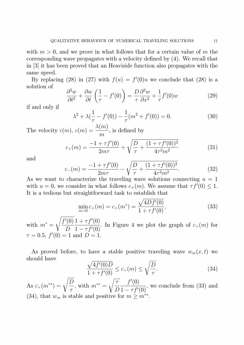
As we want to characterize the traveling wave solutions connecting u = 1with u = 0, we consider in what follows c+(m). We assume that τf ′(0) ≤ 1.It is a tedious but straightforward task to establish that

minm>0

c+(m) = c+(m∗) =

√4Df ′(0)

1 + τf ′(0), (33)

with m∗ =

√f ′(0)D

1 + τf ′(0)1− τf ′(0)

. In Figure 4 we plot the graph of c+(m) for

τ = 0.5, f ′(0) = 1 and D = 1.

As proved before, to have a stable positive traveling wave wm(x, t) weshould have √

4f ′(0)D1 + τf ′(0)

≤ c+(m) ≤√

D

τ. (34)

As c+(m∗∗) =

√D

τ, with m∗∗ =

√τ

D

f ′(0)1− τf ′(0)

, we conclude from (33) and

(34), that wm is stable and positive for m ≥ m∗∗.


0 10 20 30 40 50 60 70 80 90 1001.3

1.35

1.4

1.45

1.5

1.55

1.6

1.65

Figure 4. The graph of c+(m).

0 20 40 60 80 100 120 140 160

0.1

0.2

0.3

0.4

0.5

0.6

0.7

0.8

0.9

1

T = 75, h = 0.1, ∆ t = 0.05, D = 0.2, τ = 0.1, U = 1

Initial conditions: Heaviside (bullets); Exponential (solid)

Figure 5. Traveling waves for u0(x) = H(x) and u0(x) = em∗(−x+c+(m∗)t).

We note that traveling waves (28) with velocity c+(m) for m > 0, define afamily of solutions of the integro-differential modified problem

∂u

∂t=

D

τ

∫ t

0e−

t−sτ

∂2u

∂x2(x, s) d s + f ′(0)u + (mv+(m)− f ′(0)) e−mx− t

τ ,

(x, t) ∈ IR× IR+,

u(x, 0) = e−mx, x ∈ IR,(35)


which is equivalent to equation (29) with initial conditions

∂u

∂t(x, 0) = mc+(m)e−mx, x ∈ IR,

u(x, 0) = e−mx, x ∈ IR.

(36)

We have then constructed a family of trial functions such that, for eachadmissible velocity (34) there is an element of the family which propagateswith this velocity.

In the following we use c+(m) to study the velocity of numerical travelingwave solutions computed with Method DnRn.

To compute the numerical velocity we replace unj by a discrete traveling

wave that is a discretization of (28), that is, unj = ξnemjh, with ξ = ecn(m)k,

where cn(m) represents the velocity of the numerical wave solution obtainedby Method DnRn. We have

cn(m) =1klnξ (37)

where ξ is the solution of the following equation

ξ2 + ξ

(−2 + k

1− τf ′(0)τ

− k2

(D

τ

emh + e−mh − 2h2

+f ′(0)

τ

))

+

(1− k

1− τf ′(0)τ

)= 0.

(38)

After some computations we establish that

ξ = 1 + k

(τf ′(0)− 1

2τ± 1

2

√(1 + τf ′(0))2

τ 2+ 4

D

τm2 + O(k)

). (39)

We have then proved the following result:

Proposition 3. Let c+(m) and cn(m) represent the speed of traveling wavesolutions respectively of the integro-differential equation (3) and of differenceequation (21). Then

cn(m) = c+(m) + O(k). (40)

In Figure 6 we compare the numerical traveling wave solutions obtainedwith Method DnRn with the traveling wave defined by the Heaviside functionand with the propagation speed c+(m∗).


0 20 40 60 80 100 120 140 1600

0.1

0.2

0.3

0.4

0.5

0.6

0.7

0.8

0.9

1

T = 75, h = 0.1, ∆ t = 0.05, D = 0.2, τ = 0.1, U = 1

Figure 6. Numerical traveling wave solutions computed withMethod DnRn.

3.2. An implicit-explicit discretization.

3.2.1. Convergence and qualitative behaviour. The stability of Method DnRn

is achieved provided that the conditions (23), (24) are satisfied. These con-ditions are very severe if the reaction is stiff. In order to avoid these stabilityrestrictions we consider in the following an implicit-explicit method - MethodDn+1Rn - defined by

D2,tun+1j + D−tu

nj

(1τ− f ′(un

j )

)=

D

τD2,xu

n+1j +

1τf(un

j ), (41)

which has an amplification factor given by

|ξ| ≤ 1 +f ′(0)

1− k0f ′(0)k, (42)

provided that

k < k0 <1

f ′(0). (43)

Numerical solutions obtained with Method Dn+1Rn which show the betterstability properties of this methods are plotted in Figure 7 and Figure 8.


0 20 40 60 80 100 120 140 1600

0.1

0.2

0.3

0.4

0.5

0.6

0.7

0.8

0.9

1

T = 75, h = 0.1, ∆ t = 0.06, D = 0.2, τ = 0.1, U = 1

Figure 7. Numerical solution obtained using Method Dn+1Rn-stable behaviour.

0 20 40 60 80 100 120 140 1600

0.2

0.4

0.6

0.8

1

1.2

T = 75, h = 0.1, ∆ t = 0.0583, D = 0.2, τ = 1, U = 1

Implicit diffusion

Figure 8. Numerical solutions obtained using MethodsDn+1Rn- oscillatory behaviour.

The solutions obtained with Method Dn+1Rn present some oscillations(Figure 8). This wrong qualitative behaviour can be understood using againthe modified equation approach. The modified equation associated withMethod Dn+1Rn is defined by

−D

τk

∂3u

∂t∂x2+

∂2u

∂t2

(1 +

k

21− τf ′(0)

τ

)+

∂u

∂t

1− τf ′(0)τ

=D

τ

∂2u

∂x2+

f ′(0)τ

u,

(44)


where second order terms have been discarded. It is easy to show that theparameter p, introduced in (26), is given by

p(m) = −1− f ′(0)τ + Dk2 m2

2τ + (1− f ′(0)τ)k,

for m large enough. This expression enable us to conclude that the numericalsolution obtained with Method Dn+1Rn presents less diffusivity than thenumerical solution obtained with Method DnRn.

3.2.2. Velocity of traveling waves. Proceeding as previously we can concludethat Proposition 3 holds for Method Dn+1Rn.

4. ConclusionIn the present paper we studied the behaviour of numerical traveling waves

which are approximations to the solution of the integro-differential equation(3). We started by analyzing in Proposition 2 the well-posedness of theintegro-differential model.

The numerical methods were constructed discretizing a partial differentialequation equivalent to the integro differential equation (3). The equivalencebetween the two models was established in Proposition 1.

The first method considered was of explicit type – Method DnRn. Thismethod is stable if the stepsizes satisfy conditions (23) and (24) which arevery severe if stiff reactions are considered. This fact motivated the intro-duction of a method of implicit-explicit type – Method Dn+1Rn.

A central problem in the discrete integro-differential models is the velocityof propagation of the numerical traveling wave solutions. We established inProposition 3 that the velocity of propagation of the numerical traveling wavesolutions of Method DnRn is a first order approximation of its continuouscounterpart. The same result holds for Method Dn+1Rn.

References[1] D.G. Aronson, H.F. Weinberger, 1978, Multidimensional nonlinear diffusion in population

genetics, Adv. Math. 30,33-76.[2] J. Douglas, B.F. Jones Jr. 1962, Numerical methods for integro-differential equations of par-

abolic and hyperbolic type, Numer. Math. 4, 96-102.[3] S. Fedotov, 1998, Traveling waves in a reaction - diffusion system: diffusion with finite velocity

and Kolmogorov-Petrovski-Piskunov kinectics, Physical Review E 5, 4, 5143-5145.[4] S. Fedotov, 1999, Nonuniform reaction rate distribution for the generalized Fisher equation:

ignition ahead of the reaction front, Physical Review E 60, 4, 4958-4961.


[5] S. Fedotov, 2001, Front propagation into an unstable state of reaction-transport systems,Physical Review Letter 86, 5, 926-929.

[6] J. D. Murray, Mathematical Biology-I,II: Spatial Models and Biomedical Applications, 3 ed,2003, Springer Verlag.

[7] V. Mendez, J. Camacho, 1997, Dynamic and thermodinamics of delayed population growth,Physical Review E 55, 6, 6476-6482.

[8] V. Mendez, J. Llebot, 1997, Hyperbolic reaction-diffusion equations for a forest fire model,Physical Review E 56, 6, 6557-6563.

[9] V. Mendez, T. Pujol, J. Fort, 2002, Dispersal probability distributions and the wave frontspeed problem, Physical Review E 65, 041109.

[10] I. H. Sloan, V. Thomee, 1986, Time discretization of an integro-differential equation of para-bolic type, SIAM J. Numer. Anal. 23, 1052-1061.

[11] N.-Y Zhang, 1993, On fully discrete Galerkin approximation for partial integro-differentialequations of parabolic type, Math. Comp. 60, 201, 133-166.

A. AraujoDepartamento de Matematica, Universidade de Coimbra, 3001 - 454 Coimbra, PortugalE-mail address: [email protected]

J.A. FerreiraDepartamento de Matematica, Universidade de Coimbra, 3001 - 454 Coimbra, PortugalE-mail address: [email protected]

P. OliveiraDepartamento de Matematica, Universidade de Coimbra, 3001 - 454 Coimbra, PortugalE-mail address: [email protected]

1.Reaction-di usion equations with memory - UC · SOLUTIONS FOR REACTION-DIFFUSION EQUATIONS WITH...

Documents

Transcript of 1.Reaction-di usion equations with memory - UC · SOLUTIONS FOR REACTION-DIFFUSION EQUATIONS WITH...