Dynamic Simulation of Compressor Control Systems

Dynamic Simulation of Compressor

Control Systems

Final Thesis for the degree of

M.Sc. in Oil & Gas Technology

Submitted by

Claus Hansen

Aalborg University Esbjerg

I

Title: Final Thesis: Dynamic Simulation of Compressor Control Systems Education: Master of Science in Oil and Gas Technology Project period: February 1 – June 13, 2008 Circulation: 3 Pages: 77 Appendices: 3 Enclosed: CD-ROM Student: Claus Hansen Supervisor: Prof., Dr. Ing. Bjørn H. Hjertager Front page: Excerpts from HYSYS DynamicsTM model

Aalborg University Esbjerg Niels Bohrs vej 8 6700 Esbjerg Tlf.: +45 79 12 76 66 Fax: +45 79 12 76 76 www.aaue.dk

II

Abstract Centrifugal compressors used for gas compression are complex fluid-flow machines with a limited operational range and control of the compressors is crucial for safe and efficient operation. A model has been created for simulation of a separation and gas compression system by using HYSYS DynamicsTM. Based on the theory for centrifugal compressors and control theory a control strategy has been applied to the model based on the available equipment. The model has been used to investigate how the gas compression system responds to changes in the compressor inlet flows and conditions. The simulations performed have resulted in suggestions to modifications to the system.

Resumé Centrifugal kompressorer er komplekse maskiner, der ofte benyttes til naturgas kompression. På grund af et begrænset operationsinterval er det essentielt at regulere kompressorerne for at sikre en pålidelig og effektiv drift. En model for et separations- og gaskompressionssystem er opbygget i proces simulations-programmet HYSYS DynamicsTM. Et kompressor reguleringssystem baseret på teorien for centrifugal kompressorer og generel reguleringsteori er implementeret i modellen. Ved brug af modellen er det undersøgt hvorledes kompressionssystemet reagerer på ændringer i flow og sammensætning af gassen. På baggrund af simuleringerne er der givet forslag til modifikationer af systemet.

III

Preface This project is the Final Thesis to become Master of Science in Oil and Gas Technology. The project has been carried out in co-operation with the Process & Loss Prevention Department of Rambøll Oil & Gas in Esbjerg. The basis of the project is a detailed engineering project of an oil and gas production unit. A model has been developed using the simulation tool HYSYS DynamicsTM by AspenTech. During the project period a license for the AspenTech’s University Package for Process Modeling has been purchased which contains a comprehensive amount of programs for process simulation and among these HYSYS DynamicsTM. The first year license has been paid by Rambøll Oil and Gas, for the purpose of evaluating it as a replacement to other programs currently used at Aalborg University Esbjerg. I express my gratitude to the people at Rambøll for support and interest in my project. Especially, I would like to thank Carsten Stegelmann for guidance and constructive criticism and Asmus D. Nielsen for support, especially in matters where experience is the key. I direct my graditude to my fellow student Martin Olldag Bay for help and support throughout the project period. For referencing and citing the American Chemical Society (ACS) style along with the Name and Year System [Name, Year] has been used as described in The ACS Style Guide. [Dodd, 1997] __________________________ Claus Hansen

IV

Nomenclature A Area [m2] c Absolute gas velocity [m/s]

dC Discharge coefficient [-]

gC Gas flow sizing coefficient [USPGM]

vC Fluid flow sizing coefficient [USPGM]

pc Heat capacity at constant pressure [J/(mol·K)

d Diameter [m]

( )e t Error at sampling time t [-]

tF LMTD correction factor [-] g Gravitational acceleration [m/s2]

h Enthalpy [m2/ss]

k Constant for frictional pressure loss [-]

cK Controller gain [-]

Km Pressure recovery coefficient [-]

m& Mass flow-rate [kg/s] M Total moments of momentum [Nm] MW Moleweight [kg/kmol] N Rotational Speed [rpm]

Tn Polytropic temperature exponent [-]

nν Polytropic volume exponent [-] p Absolute pressure [bar] q Heat flow [m2/s2]

R Radius [m]

gR Universal gas constant [J/(mol·K)]

Re Reynolds’ number [-]

T Absolute temperature [K]

dT Differential time [s]

iT Integral time [s]

2sT Isentropic discharge temperature [K]

LMTΔ Log-mean temperature difference (LMTD) [K]

u Absolute blade speed [m/s] U Overall heat transfer coefficient [kJ/(K·s)] ν Molar volume [m3/mole]

V& Volume flow [m3/s]

uV Peripheral component of the absolute gas velocity [m/s]

nV Normal component of the absolute gas velocity [m/s]

V

relV Gas velocity relative to the impeller blade [m/s]

W Actual work [m2/ss]

py Polytropic head [m] or [m2/ss]

sy Isentropic head [m2/ss]

Ty Isothermal head [m2/ss]

z Elevation [m]

Z Compressibility [-] β Ratio of orifice diameter and pipe diameter [-]

ε Expansibility factor of gases [-]

κ Specific heat ratio ( /p vC C ) [-]

Tκ Isentropic temperature exponent [-]

pη Polytropic efficiency [-]

sη Isentropic efficiency [-]

Tη Isothermal efficiency [-]

Fη Friction efficiency [-]

Lη Leakage effictioency [-]

ω Angular velocity [rad/s] φ Flow coefficient, dimensionless [-] ρ Density [kg/m3] τ Fluid torque [Nm] Subscripts 1 Inner or inlet 2 Outer or outlet d Discharge s Suction

VI

Table of Contents 1 INTRODUCTION ................................................................................................................1

1.1 OBJECTIVE.................................................................................................................................................. 1 1.2 THESIS OVERVIEW...................................................................................................................................... 1

2 CENTRIFUGAL COMPRESSOR THEORY ........................................................................3

2.1 DESIGN OF CENTRIFUGAL COMPRESSORS.................................................................................................... 3 2.2 COMPRESSION PROCESS.............................................................................................................................. 6 2.3 IMPELLER CONFIGURATION ...................................................................................................................... 10 2.4 PERFORMANCE CALCULATION .................................................................................................................. 13 2.5 PERFORMANCE PHENOMENA .................................................................................................................... 19 2.6 COUPLING OF COMPRESSORS .................................................................................................................... 22

3 COMPRESSOR CONTROL ...............................................................................................24

3.1 CONTROL METHODS ................................................................................................................................. 24 3.2 GENERAL APPROACH TO COMPRESSOR CONTROL...................................................................................... 27 3.3 ANTI-SURGE CONTROL.............................................................................................................................. 29 3.4 DISTRIBUTION OF LOADS – LOAD-SHARING .............................................................................................. 31 3.5 DYNAMIC DE-COUPLING........................................................................................................................... 31

4 MODELING OF THE OGPU.............................................................................................32

4.1 DESIGN OF THE OGPU ............................................................................................................................. 32 4.2 HYSYS DYNAMICSTM MODEL ................................................................................................................... 34

5 SIMULATION SCENARIOS..............................................................................................46

5.1 SCENARIO A ............................................................................................................................................. 46 5.2 SCENARIO B.............................................................................................................................................. 49 5.3 SCENARIO C.............................................................................................................................................. 57

6 DISCUSSION......................................................................................................................61

6.1 MODIFICATIONS TO PRESENT SYSTEM ....................................................................................................... 61 6.2 FUTURE WORK.......................................................................................................................................... 62

7 CONCLUSION ...................................................................................................................63

REFERENCES ............................................................................................................................64

APPENDIX

A SIMULATION IN HYSYS

B HYSYS DYNAMICSTM PFD FOR THE OGPU

C ANTI-SURGE CONTROLLER TUNING

Introduction

1

1 Introduction Centrifugal compressors in the Oil and Gas Industry constitute a vital part of process machinery at the topside of oil and gas exploitation sites. Centrifugal compressors are expensive equipment and a major energy consumer of the processing equipment. Thus, potential for both capital and operational savings exist, if design and operation is dealt with in a competent way. In addition, centrifugal compressors are very sensitive to changes in operating conditions and have a limited operational range, and if exceeded the compressor can be damaged beyond further use. For those reasons, it is crucial that the compressors are controlled properly. The detailed design of the compressor internals is usually taken care of by experienced vendors based on the design basis, but the operation of them and interaction between serial and/or parallel coupled compressors and the equipment, to which they are connected, are not. Therefore, operability studies of the system as a whole give valuable insight into how it should be operated and controlled prior to taking it into service. In addition, alternatives to the design can be tested. Advanced compressor control include a number of possible control methods such as variable speed, suction and discharge throttling, and by-pass. The ultimate goal for compressor control is to ensure safe and economical operation while maintaining a high degree of flexibility in the system. Reliable and energy efficient anti-surge control, load-sharing strategies, and dynamic decoupling of interacting control strategies are common features of compressor control systems.

1.1 Objective This project is a study of a natural gas compression system on a designed but not yet completely built Oil and Gas Production Unit (OGPU). The design basis for the OGPU is a wellhead composition representative of the North Sea region. It is designed for a production of up to 80 000 bbl/d of liquid (maximum 60 000 bbl/d of oil or maximum 60 000 bbl/d of water) and 53 MMSCFD of gas. It is meant to be generic which means, that it must be able – perhaps with slight modifications to the design – to produce from a variety of oil and gas fields at rates at or below the above specified. A model of the OGPU processing equipment is developed using HYSYS DynamicsTM, which is a general purpose process simulation tool. The model includes main process equipment such as separators, pumps, and compressors as well as piping and valves. Details such as nozzle and vessel elevations, compressor performance curves and all vendor information readily available is applied to the model. PID controllers are added as intended in the design and it is shown how they can be tuned using generally acknowledged methods and rules of thumb and the compressor control strategy is integrated. Even though, the gas compression system is only a part of the total processing system, focus is given to this part because of its sensitivity to changes in the process conditions. The primary objective is to make the model as realistic as possible especially in regards to the control of the compressors. The model is then used to test the system under various process conditions. Based on these tests potential problems with the design are identified and modifications that can improve operability are suggested. A secondary objective is to give an example of the extensiveness in the use of HYSYS DynamicsTM as a process simulation tool. Aalborg University Esbjerg is currently evaluating whether the AspenTech University Package for Process Modeling should replace the currently used programs on the master level educations. Hence, this project can be used as part of the evaluation.

1.2 Thesis Overview The general approach in the project is process oriented using the thermodynamics to describe the compression process. However, to adequately understand the system both thermodynamics and aerodynamics are consulted

Introduction

2

and the link between them established. Beside the process oriented analysis of the compression process, strategies for advanced compressor control are described in order to set up an appropriate compressor control strategy. The present report contains a section on the theory behind centrifugal compressors. This is important in order to understand the behavior and performance of the machines. Subsequently, the theory of compressor control is described to make it possible to create a proper control system for the compressors. Hereafter the model created in HYSYS DynamicsTM is described with focus on the specific choices made for the general setup of the model. Finally, results of the various scenarios are presented and suggestions to modifications to the present design are given.

Centrifugal Compressor Theory

3

2 Centrifugal Compressor Theory Compressors are generally divided into two categories:

• Positive Displacement Compressors • Dynamic Compressors

Positive displacement compressors in essence work by entrapping a volume of gas and subsequently reducing this volume which in turn increases the pressure. Positive displacement compressors will not be covered further in this report. Dynamic compressors generally work by imparting movement to the gas; i.e. kinetic energy is transferred from the machines internals to the gas. By subsequent reduction of this velocity the kinetic energy is converted into potential energy – pressure. The two main types of dynamic compressors are:

• Axial Compressors • Centrifugal Compressors

As the name implies axial compressors impart movement to the gas in the axial direction. This is done by a series of rotors similar to those seen at the air intake in the front of jet-engines. Each rotor is followed by a stator where the kinetic energy, imparted to the gas by the rotor, is converted into pressure. Axial compressors will not be covered further in this report. Centrifugal compressors, on the other hand, work by imparting movement to the gas in radial direction by an impeller. This outward velocity is then converted into pressure in a diffuser. The main components of the compressor will be described in more detail later in this section. In this section the following subjects will be covered:

• Design of centrifugal compressors • Compressor performance • Performance phenomena • Coupling of compressors

2.1 Design of Centrifugal Compressors As mentioned above, centrifugal compressors are dynamic fluid-flow machines that can convert mechanical energy into gas energy. The increase in gas energy is expressed in an increase in pressure and temperature from inlet to outlet of the compressor. A cross-sectional view of a five-stage centrifugal compressor is shown in figure 2.1.


4

Inlet nozzle Outlet nozzle

Diffuser channel

ImpellerShaft

Collector volute

Casing

Plenum inlet

Return bend

Return inlet

Balance Piston

Labyrinth Seals

Figure 2.1. Centrifugal Compressor with five stages.

The compressor in figure 2.1 has five stages. Each compression stage consists of an impeller, a diffuser channel, a return bend, and a return inlet (or collector volute, for the last stage). Following the gas through the compressor it enters through the inlet nozzle and is distributed around the shaft in the plenum inlet. The gas is then led into the impellers where it is accelerated up to high velocities (often up to 2-300 m/s). In the diffuser channel the gas is decelerated whereby the kinetic energy is converted into potential energy – i.e. pressure. The return bend and the return inlet lead the gas on to the next stage in the compressor. After the last impeller stage the gas is collected in the collecter volute and via the outlet nozzle it is sent for further processing. Often compressors are connected in series and each compressor denoted as a stage. However, to differentiate between the internal and external number of compression steps, the internals will be referred to as stages and the entire compressor (as in figure 2.1) will be referred to as a section.

2.1.1 Main Components

In figure 2.1 the main components are named. These can be divided into stationary and dynamic components. The stationary components are those that do not move during the compression process. Stationary components include inlet and outlet nozzles, plenum inlet, diffuser channel, return bend, return inlet, collector volute, and casing. Dynamic components are those that move during the compression process. These include shaft, balance piston, and impellers. Both the stationary and the dynamic components have great effect on the efficiency of the compressor. In the following some main components that have large effects on the efficiency and performance characteristics are described.

Impellers The impellers are as mentioned before the component in which the rotational energy of the compressor is transferred to the gas. The impeller consists of a disk with blades mounted to it and usually a cover disk is


5

welded or brazed onto the impellers. In the compressor the disk is mounted onto the shaft and the gas is fed through an opening near the shaft. The factor determining the appropriate design of the impellers are the dimensionless flow coefficient defined as

24 2 2

sVd uπ

ϕ =⋅

& (2.1)

Where ϕ : Dimensionless flow coefficient

sV& : Impeller actual suction volume flow

2d : Impeller outer diameter

2u : Absolute blade tip-speed

Several impeller types exist but the most widely adapted is the shrouded 2D-impeller, which has back-ward curved blades. It has an equal curvature across the blades which are commonly referred to as 2D-blades. The shrouded 2D-impeller can handle flow coefficients in the range of 0.01 to 0.06 with reasonably high efficiencies. Beyond those limits the efficiencies are considerably reduced. For higher flow coefficients a shrouded 3D-impeller is often utilized. It has blades curved both in the radial and the axial direction leading to considerably longer blade lengths for the same diameter of the impellers. This type of impellers can handle flow coefficients up to 0.15 with reasonably high efficiencies. The shrouded 2D- and 3D-impellers can be seen in figure 2.2.

Figure 2.2. Shrouded 2D impeller to the left and shrouded 3D-impeller to the right. [Lüdtke, 2004]

The blade curvature and the influence on the overall performance will be covered further in section 2.3.1.

Labyrinth seals For each succeeding stage the pressure increases and therefore it is necessary to seal the interface between the dynamic and the stationary components. The simplest of these inter-stage seals is the labyrinth seal that work by creating turbulence in the cavities and thereby restricting flow from the high pressure side to the low pressure side. Seals of this type are favorable because there is no contact between the stationary and the moving parts; hence there is no mechanical friction or wear. The principle is shown in figure 2.3.


6

Shaft

Labyrinth seal

High pressure sideLow pressure side

Figure 2.3. Principle of a labyrinth seal at the shaft.

The seal in figure 2.3 is a knife-edge seal. The number of sealing tips in the seal depends on the application. More sealing tips gives lower leakage flow and typically interstage seals have 5-7 sealing tips, whereas the balance piston seal have 20-30 sealing tips. [Lüdtke, 2004]

Balance Piston Throughout the compressor section the pressure increases for each stage. Hence a net thrust along the shaft of the compressor exists in the direction of the compressor inlet. To outbalance the majority of this thrust a balance piston is placed after the last stage. The area behind the balance piston is connected to the inlet of the compressor with a line creating a pressure difference over the balance piston in the opposite direction. The thrust not balanced out by the balance piston is absorbed by thrust bearings.

2.2 Compression Process The compression process can be described by use of either thermodynamics or aerodynamics. The former is a macroscopic description of the compression process and can be used to describe the overall performance. The latter is a microscopic description that can be used to explain performance phenomena such as surge and stonewall and to explain overall performance characteristics. In the following, both the thermodynamic and the aerodynamic explanation will be given and the link between them established.

2.2.1 Thermodynamics

The general energy balance for compressors may be written in differential form as

2

2cdy dq dh d g dz+ = + + ⋅ (2.2)

Where y : Specific mass referenced compressor work input

q : Heat flow into the compressor through walls

h : Enthalpy of gas c : Absolute gas velocity g : Gravitational acceleration

z : Elevation

Leakage Gas Flow


7

Thus, the sum of the specific mass referenced work input and the heat flow to the compressor is equal to the sum of the enthalpy change, the kinetic energy change, and the static head difference. Usually the velocity term and the static head contributions are regarded negligible and the compressor is considered adiabatically isolated from the environment. Hence equation 2.2 reduces to

dy dh= (2.3)

The change in enthalpy of the gas is

dpdhρ

= (2.4)

Where ρ : Density of the gas

p : Pressure of the gas

The specific compressor mass referenced work input is then

2

1

p

p

dpyρ

= ∫ (2.5)

The actual work is found by dividing the mass referenced work input by an efficiency

yWη

= (2.6)

Where W: Actual work applied to the compressor The integral in 2.5 can be solved in different ways equivalent to different compression paths. Usually, one of three different reference processes for compression is used to solve compressor performance. These are

• Isentropic compression (reversible and adiabatic) – entropy is constant • Isothermal compression (reversible and diathermic) – temperature is constant • Polytropic compression (irreversible and adiabatic) – efficiency is constant

Reference process – Isentropic compression If there is no heat transfer to or from the gas being compressed the process is adiabatic and isentropic. For such a process the compression path is dependent on

1

11

. .p pp const const

p

κκ

κν ρ ρρ

⎛ ⎞⋅ = ⇒ = ⇒ = ⋅⎜ ⎟

⎝ ⎠ (2.7)

Where ν : Molar volume κ : Specific heat ratio ( /p vC C )

Inserting the above expression for the density in equation 2.5 and integrating gives

2

1

11

1 1 21

1 1 1

11

p

sp

p dp p pypp

κκ κ

κ

κρ ρ κ

−⎡ ⎤⎛ ⎞⎢ ⎥= ⋅ = ⋅ ⋅ −⎜ ⎟⎢ ⎥− ⎝ ⎠⎢ ⎥⎣ ⎦∫ (2.8)

Where sy : Isentropic head

Insering / /gp ZR T MWρ = into equation 2.8 gives


8

1

1 1 2

1

11

gs

Z R T pyMW p

κκκ

κ

−⎡ ⎤⋅ ⋅ ⎛ ⎞⎢ ⎥= ⋅ ⋅ −⎜ ⎟⎢ ⎥− ⎝ ⎠⎢ ⎥⎣ ⎦

(2.9)

Where Z : Compressibility gR : Gas constant

T : Absolute temperature MW : Moleweight of the gas

Reference process – Isothermal compression If heat is removed continuously during the compression process the isothermal compression process may be approached. In this case

11

. .p pp const const

pν ρ ρ

ρ⎛ ⎞

⋅ = ⇒ = ⇒ = ⋅⎜ ⎟⎝ ⎠

(2.10)

This simple relation gives a much simpler integration and the isothermal head is

1 1 2

1

lnTR T Z py

MW p⎛ ⎞⋅ ⋅

= ⋅ ⎜ ⎟⎝ ⎠

(2.11)

Where Ty : Isothermal head

Reference process – Polytropic compression Usually compressors are neither isentropic nor isothermal, but instead they are best described by a polytropic compression path given by

1

11

. .n

nnp pp const const

p

νν

νν ρ ρ

ρ⎛ ⎞

⋅ = ⇒ = ⇒ = ⋅⎜ ⎟⎝ ⎠

(2.12)

Where nν : Polytropic volume exponent

Inserting this in equation 2.5 and integrating gives

1

1 1 2

1

11

nn

pnZ R T Py

MW n P

ν

νν

ν

−⎡ ⎤⎛ ⎞⋅ ⋅ ⎢ ⎥= ⋅ −⎜ ⎟⎢ ⎥− ⎝ ⎠⎢ ⎥⎣ ⎦

(2.13)

Where py : Polytropic head

Actual compression process The choice of reference compression process depends on the actual compression process to be described. Thus, for compression processes that are close to isentropic, which is the case with many intercooled compression processes where the gas behaves almost ideally, the isentropic reference process should be selected. In cases where the intercooling is so significant that the process can be considered isothermal the performance is best described by the use of this reference process. However, for most applications – in particular as the compressors grow larger – the compression process is neither isentropic nor diathermic, and in such situations the compression process is most accurately described by application of the polytropic compression path. Note that in the polytropic compression path the efficiency is assumed equal for all internal stages of the compressor. This


9

is the truth for most compressors within a margin of 1 % of and is as such a reasonable approximation. [Lüdtke, 2004] It should be noted that eventhough the polytropic reference process is adiabatic it is not reversible. This is due to a friction caused entropy increase in the process which is irreversible. The reference processes are all related to the actual work applied to the compressor by

p s T

p s T

y y yWη η η

= = = (2.14)

Where pη : Polytropic efficiency

sη : Isentropic efficiency

pη : Isothermal efficiency

In these efficiencies lie losses caused by friction and leakage and they should always be supplied together with the head curves.

2.2.2 Aerodynamics

The aerodynamic explanation to the enthalpy change experienced by the fluid in the impeller section is best described by derivation of the Euler Turbomachinery Equation; hence this is done in the following. The derivation is based on the assumption that the single compressor stage can be regarded as adiabatically isolated from the environment. Figure 2.4 is a cross section of the flow path from the return inlet through the impeller and into the diffuser.

1

2

R

R

1

2

nVDiffuser

Impeller

Return inlet

Shaftw

Figure 2.4. Flow of gas through the impeller. Vn: normal gas velocity, R: radius, ω: angular velocity.

Setting up a control volume over the impeller from inlet (1) to outlet (2), the total moments of momentum entering and leaving the control volume is given by

Vn


10

1 1

2 2

1 1 1 1

2 2 2 2

d

d

n u

n u

M V V R A

M V V R A

ρ

ρ

= ⋅ ⋅ ⋅ ⋅

= − ⋅ ⋅ ⋅ ⋅

∫∫

(2.15)

Where M : Total moments of momentum nV : Normal component of the absolute gas velocity

uV : Peripheral component of the absolute gas velocity

R : Radius from centre of rotation dA : Elemental area of flow The fluid torque is the net effect of the moments of momentum equal to

1 1 2 21 1 1 2 2 2d dn u n uV V R A V V R Aτ ρ ρ= ⋅ ⋅ ⋅ ⋅ − ⋅ ⋅ ⋅ ⋅∫ ∫ (2.16)

Where τ : Fluid torque The mass flow rate at steady state is given by

1 21 1 2 2d dn nm V A V Aρ ρ= ⋅ ⋅ = ⋅ ⋅∫ ∫& (2.17)

Where m& : Mass flow rate If it is assumed that uV R⋅ is constant then equation 2.16 and 2.17 can be combined to give

( )1 21 2u um V R V Rτ = ⋅ − ⋅& (2.18)

By multiplying equation 2.18 by the angular velocity and rearranging one form of the Euler turbomachinery equation specific for compressors emerges [Turton, 1995]

1 2

1 2

1 2

1 2

u u

u u

V R V Rmy V u V u

τ ω ω ω⋅= ⋅ ⋅ − ⋅ ⋅

− = ⋅ − ⋅& (2.19)

Where ω : Angular velocity u : Absolute peripheral velocity of the rotor The minus sign in front of the mass referenced work input is there because for compressors the work done by the gas is negative. Changing the sign gives the specific mass referenced work for compressors [Lüdtke, 2004]

2 12 1u uy V u V u= ⋅ − ⋅ (2.20)

Thus, it has been shown how the aerodynamics is linked to the thermodynamics. In section 2.4 it will be shown how the performance can be calculated from polytropic head and efficiency.

2.3 Impeller configuration As it is evident from the previous section it is in the impellers that the energy is converted from mechanical energy to gas energy. Hence, the impeller configuration has a great effect on the overall performance of the compressor. In the following some general strategies for arranging the internals of the impellers and arranging the impellers on the compressor shaft will be described and the effect on the compressor performance is given.

2.3.1 Impeller types

In general impellers have three different configurations:


11

Rotation

c Vrel Vrel Vrel

u2u2 u =V2Vu2 u2 Vu2R2

R1

Vn=Vn Vn

c2 2

2c

22

2

• Forward leaning • Radial • Backward leaning

The performance of these three types of impellers can best be understood by looking at the aerodynamics at the impeller tips in terms of velocity vectors. In figure 2.5 the three situations are depicted schematically with the resulting velocity vectors.

Figure 2.5. Forward leaning, radial, and backward leaning impellers.

The velocity vectors in figure 2.5 are depicted at radius 2R (i.e. the outlet of the impeller). Similar vectors could be depicted at radius 1R (i.e. the inlet of the impeller) only these would be different in magnitude. The normal velocity,

2nV , the peripheral velocity, 2uV , and the absolute blade tip speed, 2u , were all introduced in section

2.2.2. The absolute gas velocity can be defined by

2 22 2u n relc V V u V= + = + (2.21)

Where 2c : The absolute gas velocity

relV : The gas velocity relative to the impeller blade

Now consider a situation where the peripheral component of the inlet velocity, 1uV , is zero, called zero the

inlet whirl. Then the aerodynamic expression for the mass referenced specific head in equation 2.20 reduces to

2 2ideal uy V u= ⋅ (2.22)

The situation is of course not possible as it would require that the gas was fed at the centerpoint of the impeller which is impossible. However, the ideal head serve to explain the basic shape of the head curves for compressors with the three different impeller configurations listed previously. Since the velocity relative to the impeller blades, relV , is proportional to flow it can be stated that for radial bladed impellers 2u is equal to

2uV no matter the flow and therefore the ideal theoretical head curve is flat. For forward leaning impeller blades

2uV increases as the flow and thereby relV increases. Hence the ideal theoretical compressor curve for compressors with forward leaning impeller blades is one with a positive slope. For compressors with backward leaning impellers

2uV decreases with flow and therefore the ideal theoretical compressor curve has a negative slope. The ideal and typical performance characteristics for the three impeller types are shown in figure 2.5.


12

Actual Volume Flow

Head

Actual Volume Flow

Head

Actual Volume Flow

Head

Figure 2.6. Typical head curves (solid line) for the compressors with forward leaning, radial, and backward leaning impellers. The dashed lines are the ideal theoretical head curves for the zero inlet whirl situation.

The vertical distance between the ideal theoretical head curves and the actual performance curves describe the losses due to friction, leakage, and incidence. Usually backward leaning impellers are used because they generally give the best efficiency in the largest flow interval; i.e. the actual head curve is closest to the ideal head curve in this type of impeller compared to radial and forward leaning impellers. Forward leaning impellers are often used when the requirement of head is dominant because this impeller type can deliver a given minimum head in a larger flow interval than the other two impeller types.

2.3.2 Impeller arrangement – in-line and back-to-back

The traditionally used impeller arrangement is in-line – also called straight through arrangement – where one stage after the other is placed on the shaft. This configuration can be seen on figure 2.1. As described previously the balance piston acts by balancing thrust by use of a connecting line from inlet to the area behind the balance piston. Since the seals at the balance piston are not completely tight a leakage flow will pass through all the stages of the compressor. Thereby extra gas power is consumed. The size of the power loss is relatively high for straight through compressors – roughly between 1 and 3.5 %, depending on pressure ratio of the compressor. [Lüdtke, 2004] The straight through compressor arrangement with the path of the recirculating flow is shown in figure 2.7.

Gas inlet Gas outlet

Line connectingarea behindbalance pistonto gas inlet

RecirculatingFlow

Figure 2.7. Straight through compressor arrangement


13

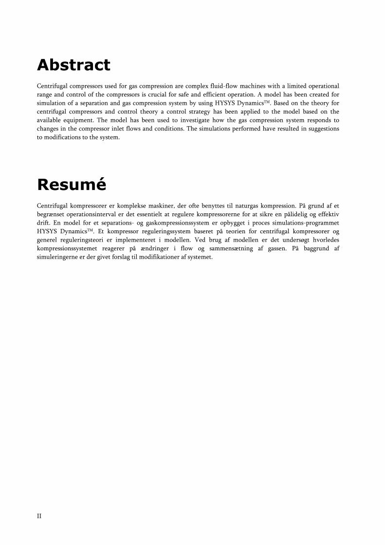
As an alternative to the in-line impeller arrangement a back-to-back impeller arrangement can be utilized. The idea is to place two sections in the same casing with the outlets adjacent to each other and with an intercooler between the sections. This arrangement is depicted schematically in figure 2.8.

Section 1 Section 2

Intercooler

Gas outletGas inlet

Recirculating flow

Figure 2.8. Back-to-back compressor arrangement.

The advantage of back-to-back configuration to in-line impeller configuration is that the balance piston is replaced by a rudimentary labyrinth seal between the outlet stages of each section. Thus, the leakage flow is only re-circulated through the latter section of the back-to-back compressor. In result the compressor power loss due to leakage is reduced to approximately one third of the power loss in the in-line impeller configuration. Another advantage is that the greatest part of the impeller thrust is out-balanced by the impellers themselves. [Lüdtke, 2004]

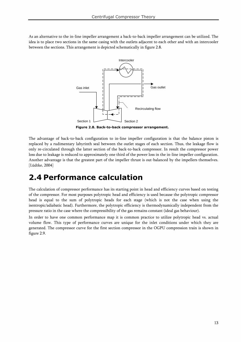
2.4 Performance calculation The calculation of compressor performance has its starting point in head and efficiency curves based on testing of the compressor. For most purposes polytropic head and efficiency is used because the polytropic compressor head is equal to the sum of polytropic heads for each stage (which is not the case when using the isentropic/adiabatic head). Furthermore, the polytropic efficiency is thermodynamically independent from the pressure ratio in the case where the compressibility of the gas remains constant (ideal gas behaviour). In order to have one common performance map it is common practice to utilize polytropic head vs. actual volume flow. This type of performance curves are unique for the inlet conditions under which they are generated. The compressor curve for the first section compressor in the OGPU compression train is shown in figure 2.9.


14

Polytropic Head

Polytropic Efficiency

10000

11000

12000

13000

14000

15000

16000

17000

18000

19000

20000

2400 2600 2800 3000 3200 3400 3600 3800 4000 4200

Actual Volume Flow [m³/h]

Hea

d [

m]

68

69

70

71

72

73

74

75

76

77

78

Eff

icie

ncy

[%

]

Figure 2.9. Polytropic Head/Efficiency vs. Actual volume flow. Similar curves for the second and third stage compressors can be found in the Excel worksheet “Compressor.xls” on the CD-ROM. Head vs. actual volume flow curves are used because it is believed that the compressor always deliver the same head at the same actual inlet volume flow. This is also what the Euler equation states. However, when there are significant compressibility changes in the flow which is generally the case when the tip-speed Mach numbers are above 0.4 and there are more than two compressor stages, the head can vary. The factors that cause the polytropic head to vary are parameters that affect the Mach number, i.e. compressor rotational speed, suction temperature, and gas composition. These effects are called aerodynamic stage mismatching and will be further discussed in section 2.5.3. [Lüdtke, 2004]

2.4.1 Polytropic change of state

In the following it is shown how polytropic head/efficiency curves can be used to calculate discharge conditions based on the inlet conditions. The formulas presented are for real gases but strictly speaking only valid for the exact conditions under which the polytropic head/efficiency curves have been found. However, for slight changes in the inlet conditions reasonably accurate results can be obtained, and certainly the general effect of changing the inlet conditions can be deduced. The starting point for polytropic processes is the relation the equation for polytropic head deduced in section 2.2.1. In the following it is shown how outlet temperature, pressure, and volume flow for real gases can be calculated based on the polytropic head and efficiency curves. The prerequisite for the calculations are that it is possible to calculate all thermodynamic properties from an equation of state (e.g. Peng-Robinson).

Pressure The polytropic head for compression of real gases expressed in the unit of length is given by equation 2.23.

1

1 1 2

1

11

nn

pnZ R T Py

MW g n P

ν

νν

ν

−⎡ ⎤⎛ ⎞⋅ ⋅ ⎢ ⎥= ⋅ −⎜ ⎟⎢ ⎥⋅ − ⎝ ⎠⎢ ⎥⎣ ⎦

(2.23)


15

Isolating the discharge pressure 2p gives equation 2.24.

1

2 11 1

11

nnpy MW g np p

Z R T n

ν

νν

ν

⎛ ⎞⎜ ⎟⎜ ⎟−⎝ ⎠⋅ ⋅⎡ ⎤−

= ⋅ + ⋅⎢ ⎥⋅ ⋅⎣ ⎦ (2.24)

Thus the discharge pressure is a function of suction pressure, compressor head, and the composition.

Temperature Recalling that the definition of a polytropic process is

.np constνν⋅ = (2.25)

Rearranging equation 2.25 by using /ZRT Pν = gives the expression in equation 2.26 [Lüdtke, 2004].

11

T

T TT

T T

nn nn m

n np pT Pp const const

P T T T

−−

= → = = = , where 1T

T

nmn−

= (2.26)

Tn is the polytropic temperature exponent and is different from the polytropic volume exponent. In equation 2.26 the compressibility is assumed constant. Using the relation in 2.26 allow for calculation of the discharge temperature as shown in 2.27.

1 2 22 1

1 2 1

mm mp p pT TT T p

⎛ ⎞= ⇔ = ⋅⎜ ⎟

⎝ ⎠ (2.27)

m – and thereby the polytropic temperature exponent, Tn – is calculated by equation 2.28 [Lüdtke, 2004].

1 11 1 T

p p T

Z Rmc

κη κ

⎛ ⎞⋅ −= ⋅ − +⎜ ⎟⎜ ⎟

⎝ ⎠ (2.28)

Where Tκ : Isentropic temperature exponent defined at constant entropy ( 1pη = )

pc : Heat capacity at constant pressure

The isentropic discharge temperature, 2sT , is given – similarly to 2.27 – by equation 2.29.

1

22 1

1

T

T

spT Tp

κκ−

⎛ ⎞= ⋅⎜ ⎟

⎝ ⎠ (2.29)

Rearranging equation 2.29 gives

2

1

2

1

log1

log

s

T

T

TTpp

κκ

⎛ ⎞⎜ ⎟

− ⎝ ⎠=⎛ ⎞⎜ ⎟⎝ ⎠

(2.30)

Combining equations 2.27, 2.28 and 2.30 gives

22 1

1

mpT Tp

⎛ ⎞= ⋅⎜ ⎟

⎝ ⎠, where

2

1

2

1

log1 1

log

s

p p

TTZ Rm

c pp

η

⎛ ⎞⎜ ⎟⎛ ⎞⋅ ⎝ ⎠= ⋅ − −⎜ ⎟⎜ ⎟ ⎛ ⎞⎝ ⎠ ⎜ ⎟⎝ ⎠

(2.31)


16

The isentropic discharge temperature is found by the equation of state.

Volume The actual volume flow of the discharge stream is calculated by

12 1

2

V V ρρ

= ⋅& & (2.32)

Where ρ : Density at suction (1) and discharge (2)

V& : Actual volume flow at suction (1) and discharge (2) Here the density is found from the equation of state.

2.4.2 Calculation scheme

For calculation of the performance – i.e. discharge pressure and temperature – under different operating conditions have been computed accordingly to the calculation scheme given in figure 2.10.


17

Figure 2.10. Calculation scheme.

A program has been written in the Visual Basic application for Excel using the calculation scheme in figure 2.10 to calculate compressor performance with starting point in compressor curves similar to that of figure 2.9 (cf. “Compressor.xls” on CD-ROM).

2.4.3 Operating characteristics

Using the calculation scheme shown in figure 2.10 it is possible to predict the operation characteristics under different operating conditions. In figure 2.11, 2.12, and 2.13 the Influence of the performance at different moleweights, suction temperatures, and suction pressures are shown using the performance curves of the first section compressors seen in figure 2.9. In all cases the equation of state used is Peng-Robinson.

Set: 1 1, , ,p T Composition and &m

Calculate: 1 1 1and , ,ρMW Z V by EOS

Set Polytropic Head and Polytropic efficiency by 1V

Calculate 2P

Guess: νn and Tn

Calculate 1 1 2 2ν= ⋅ − ⋅& & vn nD p V p V

Calculate 2ρ by EOS

Calculate m

Calculate 2sT by EOS

Is 1210 ?−<D

Adjust nν by secant-method

Calculate 2&V

No YesSTOP!


18

25

30

35

40

45

50

24000 29000 34000 39000

Mass Flow [kg/hr]

Dis

ch

arg

e P

ressu

re [

bara

]

M W = 22.5 M W = 23 M W = 23.5 M W = 24 M W = 24.5

125

130

135

140

145

150

155

160

165

170

24000 29000 34000 39000

Mass Flow [kg/hr]

Dis

ch

arg

e T

em

pera

ture

[°C

]

M W = 22.5 M W = 23 M W = 23.5 M W = 24 M W = 24.5

Figure 2.11. Discharge pressure and discharge temperature as a function of mass flow at different moleweights (P1=10.3 bara, T1 = 40 °C)

25

30

35

40

45

50

24000 29000 34000 39000

Mass Flow [kg/hr]

Dis

ch

arg

e P

ressu

re [

bara

]

T1 = 30 T1 = 35 T1 = 40 T1 = 45 T1 = 50

129.5

134.5

139.5

144.5

149.5

154.5

159.5

164.5

169.5

24000 29000 34000 39000

Mass Flow [kg/hr]

Dis

ch

arg

e T

em

pera

ture

[°C

]T1 = 30 T1 = 35 T1 = 40 T1 = 45 T1 = 50

Figure 2.12. Discharge pressure and discharge temperature as a function of mass flow at different suction temperatures (MW=23.5 g/mole, P1=10.3 bara)

15

20

25

30

35

40

45

50

24000 29000 34000 39000

Mass Flow [kg/hr]

Dis

ch

arg

e P

ressu

re [

bara

]

P1 = 9.3 P1 = 9.8 P1 = 10.3 P1 = 10.8 P1 = 11.3

112.2

122.2

132.2

142.2

152.2

162.2

24000 29000 34000 39000

Mass Flow [kg/hr]

Dis

ch

arg

e T

em

pera

ture

[°C

]

P1 = 9.3 P1 = 9.8 P1 = 10.3 P1 = 10.8 P1 = 11.3

Figure 2.13. Discharge pressure and discharge temperature as a function of mass flow at different suction pressures (MW=23.5 g/mole, T1=40 °C)

As seen on the graphs in figure 2.11 through 2.13 relatively small deviations in the inlet conditions have great impact on the discharge pressures as well as temperatures.


19

2.5 Performance phenomena Generally there are two phenomena that limit the performance of the compressor. These are,

• Surge • Stonewall

Surge is the lower boundary of a stable flow and stonewall is the upper limit of the compressor flow. In addition to this the effect of stage mismatching should be considered when altering the inlet conditions. In the following these three phenomena will be explained.

2.5.1 Surge

Surge can happen on two different levels. Stage surge is surge in a single stage of the compressor whereas system surge is when the entire system goes into surge. Although the phenomena are similar with regard to causes the implications are somewhat different.

Stage surge In figure 2.14 the flow through the impeller is depicted under normal operation and at stage surge.

Rotation

Impeller bladeU

Vrel

2

Vgas

aPropagationof Stage SurgeU

Vrel

2

Vgas

i

Flow separation

(a) Normal Operation (b) Stage surge

Figure 2.14. Flow patterns in an impeller at normal operation and at stage surge. a: flow angle, i: incidence angle, Vrel: gas velocity relative to impeller blade, u2: impeller blade tip speed, Vgas: velocity of gas.

As depicted in figure 2.14(a) the gas flows through the ducts between the impeller blades under normal operation. However, when flow is reduced – or rotating velocity is increased at constant flow – the flow angle is decreased. This means that each gas molecule must travel a longer distance and more of the flow momentum is dissipated by friction at the impeller blades. At the same time the incidence angle at the impeller inlet is increased which causes flow separation at the low pressure side of the impellers as depicted in figure 2.14(b). The flow separation tends to continuously shift round the diffuser from one impeller blade to the next in the opposite direction of the rotation. [Gresh, 2001]


20

Volume Flow

P

AB

CA' B'

C'

DD'

E'F

Quadrant IQuadrant II

E

Quadrant IVQuadrant III

The flow separation due to poor incidence angle leads to flow reversal and the stage will exhibit flow and pressure fluctuations around a mean value. These pressure and flow fluctuations are known as stage surge. The stage surge condition can be present both at the impellers and in the stationary flow channels, but the effect is similar. Stage surge occurs at low flow just before system surge occurs, but if operating conditions remain constant it is a stable compressor operating condition with a net forward flow. However, for the component experiencing this flow condition it is a dynamic instability, which can cause damage to the components under influence. [Lüdtke, 2004]

System Surge As mentioned above system surge is a condition that occurs if flow is lowered even more in a condition of stage surge. However, system surge can also occur without a preliminary stage surge. The aerodynamic explanation to the condition is similar to that explained for stage surge, but the implications of a system surge are much more severe as all components in the compressor can be damaged beyond the point where operation of the compressor is possible. In system surge it is not a local flow reversal at an impeller or in the flow channels, but flow reversal through the entire compressor. System surge is best described by extending the operating curve into the second quadrant as depicted schematically in figure 2.15.

Figure 2.15. Performance curve extended into the second quadrant. [Lüdtke, 2004]

Imagining a system with a pressurized gas reservoir at the outlet of the compressor the following reasoning for operating points A, B, and C can be made with reference to the curve in figure 2.15:

1. If the operation point shifts from A to B the reservoir momentarily deliver the difference A BV V−& & which lower the pressure of the reservoir and thereby restores the former operating point, A.

2. If the operation point shifts from A to C the reservoir momentarily stores the difference C AV V−& & which increase the pressure of the reservoir and thereby restores the former operating point, A.

Thus, condition A is a stable operating point and in this part of the performance curve the system is to a large extent self-controlled. Similar reasoning for A’, B’, and C’ give different results:

&V


21

3. If the operation point shifts from A’ to B’ the reservoir momentarily stores the difference ' 'B AV V−& & which increases the pressure of the reservoir and thereby moves the operating point further away from A’. On the path from A’ to D the compressor continuously pumps more flow into the reservoir, but as D is reached and the pressure still increases due to the increase in flow, the only possible way is for the compressor instantaneously to shift to operating point D’. This reverses the flow and the reservoir begins to unload and the operating point moves towards E’. Further pressure reduction is only possible if the operating point shifts to E, and from here the reservoir begins to fill increasing the pressure, and thus moving the operating point towards D. From here the cycle DD’EE’D begins once again.

4. Similar reasoning can be made if the operating point shifts from A’ to C’. The result is a flow cycle E’EDD’E’.

Therefore, condition A’ is an unstable operating point. [Lüdtke, 2004] The consequence of this is that stable operation can only be achieved of the flow is greater than that of point D.

2.5.2 Stonewall

The other limit to normal operation of a compressor is called stonewall. The phenomenon is characterized by the sonic gas velocity at the impeller blade inlet. It occurs when the system resistance decreases and flow thereby increases. For a single stage compressor stonewall occurs when the head becomes zero, but for multistage compressors the situation is different. As the inlet flow to the compressor increases each subsequent stage sees a disproportional flow increase. That is, the relative flow increase becomes larger for each subsequent stage. Therefore, as flow increases, the first stage in which zero head occur, is the last stage of the compressor. Thus, the compressor flow limit – i.e. stonewall – is determined by the last compression stage. In figure 2.16, the situation is depicted schematically for a five stage compressor.

Volume Flow

Head

Stonewall

12

34

5

Total compressor head curve

Normal operating point

Stage curves

Figure 2.16. Individual stage head curves and total compressor curve for a five stage compressor. The total head curve is the sum of heads of the individual stages.

A multi-stage compressor subjected to an ever decreasing system resistance can in certain cases operate stably beyond stonewall. In this case the initial stages produce head and the later stages consume the head. However, especially thrust bearings in the compressor must be sized accordingly, because thrust variations throughout the


22

stages of the compressor will be inevitable. Although, stable operation can be achieved it should be avoided because it is a situation where much of the enthalpy created in the first stages are transferred to unavailable energy – heat – in the later stages. [Lüdtke, 2004]

2.5.3 Aerodynamic stage mismatching

The effect of aerodynamic mismatching stem from the fact, that there is a non-linear progressive shift in the actual volume flow for each subsequent stage in a compressor section. If for instance the volume flow at the first stage is reduced by 5 % then the volume flow will be reduced by more than 5 % in the subsequent stage and even more for each stage hereafter. Similarly if flow is increased at the first stage then each stage hereafter sees an even higher percentage-wise increase in the flow. When operating the compressor under the conditions specified for the performance map delivered by the compressor manufacturer the stage mismatching effects are included implicitly in the efficiency data. However, when deviating from design conditions the mismatching effects are among others responsible for efficiency degradation, deviations from fan laws, and distortion of the surge limit. The aerodynamic stage mismatching or compressibility change between stages is basically brought about by any change in the stage inlet conditions. Thus, variation in compressor speed and composition, flow, and temperature of the inlet stream lead to stage mismatching. The effects of stage mismatching are present whenever there is an appreciable compressibility in the flow which is generally the case for impeller tip-speed Mach numbers above 0.4. Below this threshold the stage mismatching effects can be considered to be negligible. [Lüdtke, 1998]

2.6 Coupling of Compressors Coupling of compressors can be either serial of parallel. The implications of these couplings will be described in the following.

2.6.1 Serial

In essence serial coupling of compressors are similar to the division of stages. However, one major difference between the internal stages of a compressor and serial coupling of two or more compressors is that the gas is usually not cooled between stages, whereas cooling is usually done between sections. Curves for the three serial connected compressors at the OGPU and the resulting total head curve are shown in figure 2.17.


23

0

5000

10000

15000

20000

25000

30000

35000

40000

45000

0 0.2 0.4 0.6 0.8 1 1.2

Actual Volume Flow [m³/s]

He

ad [

m]

Figure 2.17. Polytropic head curves for the three serial connected compressors on the OGPU and the resulting total polytropic head curve.

As explained in section 2.5.2 each succeeding stage sees a disproportional change in flow as the inlet flow is increased or decreased. Similar reasoning can be made for compressors connected in series, and hence surge or stonewall is most liable to occur at later sections as the flow is changed at the inlet of the first section. Hence, surge can be expected to occur first in the last section and last in the first section.

2.6.2 Parallel

Compressors are often coupled in parallel in order to have a large turn-down ratio. Parallel connection of compressors mainly affects the ability of the system to adapt to different flows. However, one major implication to the control of the compression system is that inlets and outlets are in open connection to each other and therefore pressures are balanced. Since it is impossible to construct compressors exactly similar and because it is inevitable that piping etc. around the compressors are different, the parallel connections calls for a system to balance the load on the compressors. This is called load-sharing and will be treated further in section 3.4.

1

2 3 Sections

Total Head

Compressor Control

24

3 Compressor Control Compressors are to some extent self-controlled when operating in the stable area of the performance curve as described in section 2.5. However, to avoid operating in unstable areas of the performance curve, and to enable off-design operation, compressor control must be integrated into the system. In this section the following subjects are covered

• Control methods • General approach to compressor control

Subsequently, methods to enable essential capabilities of the overall control system will be described. These are

• Anti-surge control • Distribution of loads – i.e. load-sharing • Dynamic de-coupling

The reason to employ anti-surge control and load-sharing capability are evident from the descriptions in section 2.5 and 2.6. Dynamic de-coupling must be employed to eliminate regions of instability where control strategies that are interactive can create unstable process oscillations.

3.1 Control methods Four widely used control methods for controlling the performance of compressors are

• Variable speed control • Suction throttling • Adjustable Inlet Guide Vanes (IGV) • By-pass – Discharge throttling

The function of these control methods is to extend the operating range of the compressor beyond the single performance curve (as depicted in figure 2.9) and to a so-called performance map. As seen from the following this extension can be made with variable success in regards to maintain a high efficiency on the compressor.

3.1.1 Variable speed control

Variable speed control of compressors rely on the aerodynamic relationships called fan laws stating that

( )2 2 222 1

1

, , ln ,ppV N y N N T T Np

⎛ ⎞∝ ∝ ∝ − ∝⎜ ⎟

⎝ ⎠& (3.33)

Where N : Rotational speed These relationships can be deduced from aerodynamics by assuming an ideal gas and a single stage compressor. Thus, for actual systems with real gases and multiple compressor stages, the accuracy of the relationships are somewhat reduced. However, they serve as a mean to show what can be expected when reducing or increasing speed of the compressor. A graphical representation of the fan laws are shown in figure 3.18. [Gresh, 2001]

Compressor Control

25

100%

110%

90%

80%

0

5000

10000

15000

20000

25000

1500 2000 2500 3000 3500 4000 4500 5000

Actual Volume Flow [m³/hr]

Poly

tropic

Head [

m]

Figure 3.18. Application of fan laws on the first section compressor curves of the OGPU at speeds of 80-110 % of design speed.

As stated above the fan laws are applicable to ideal gases and single stage compressors, only. The implications of real gases and multiple stage compressors are the effect of aerodynamic stage mismatching as explained in section 2.5.3. The effect of stage mismatching on the head curves as shown in figure 3.18 is that the 80 and 90 % curves in reality lie lower and farther to the left, and the 110 % line lie farther up and to the right. Advantages to using variable speed to control compressor performance are:

• High part-load efficiencies (>95 % of design efficiency) as compressor only produce the head necessary in part-load situations

• Possible to overload the system (by volume flow) because of over-speed • Suitable for all compressor types

The main disadvantage is that a driver with variable speed is required. However, for most applications variable speed control is the first choice. [Lüdtke, 2004]

3.1.2 Suction Throttling

A throttling valve installed at the suction side can be regarded as an integral part of the compressor. When doing so the performance map for the compressor is similar to the one shown in figure 2.13, – i.e. the outlet pressure is proportional to the inlet pressure. However, the compressor head curve seen from downstream the throttling valve discharge is the unaltered performance curve. Advantages to suction throttling are

• Suitable to all compressor types • Relatively low investment costs as compared to e.g. variable speed control

Main disadvantages are

Compressor Control

26

• Low efficiency at part-load due to energy loss in throttling valve • Overload not possible

However, the low efficiency at part-load, suction throttling is widely used especially due to its simplicity and low investment costs. [Lüdtke, 2004]

3.1.3 Adjustable Inlet Guide Vanes (IGV)

Adjustment of IGV’s is a real compressor head variation as opposed to suction throttling. According to the Euler turbomachinery equation (see equation 2.20) the polytropic head is a function of the peripheral gas velocity at the impeller inlet (

1uV ). By adjusting the inlet guide vanes the incidence angle at the impeller inlet can be altered and thus the peripheral velocity changed. An important property of IGV’s is that only the pertaining impeller performance is influenced. In principle guide vanes can be inserted at the inlet of each stage, but due to lack of space, multistage compressors are normally only equipped with one set of IGV’s. If the compressor is integrally geared more space is often available and hence more IGV’s can be installed in those situations. The effect of adjustable inlet guide vanes is strongest for backward leaning impeller blades, because here the peripheral speed at the impeller outlet (

2uV ) is lowest (cf. equation 2.20 and figure 2.5).

Advantages to the adjustable IGV’s are

• Medium part-load efficiencies (lower than variable speed, higher than suction throttling) • With negative prerotation of the IGV’s it is possible to overload

Main disadvantages are

• Higher investment costs than e.g. suction throttling

The use of adjustable IGV’s is mainly in situations where it is possible to fit IGV’s at more than one stage (i.e. in integrally geared compressors).

3.1.4 By-pass – Discharge Throttling

By-pass control is also referred to as discharge throttling. Flow is by-passed from the compressor discharge to the compressor inlet through a valve. If the recycle is regarded as an integral part of the compressor, then the performance map expands all the way to zero flow (i.e. full recycle). However, as the compressor in reality only have one performance curve the energy input remains constant. Advantages to by-pass control are

• Suitable for all compressor and impeller types • Simple control with low investment cost • Possible to extend the performance map to zero flow – i.e. full recycle

The main disadvantage is of course

• High energy cost at part-load • Impossible to overload

Because by-pass is the only control method that expands the performance map to zero flow it is always an integral part of the compressor control system.

Compressor Control

27

3.2 General approach to compressor control The polytropic head/efficiency vs. actual volume flow curves are, as described in section 2.4, constant for a given set of inlet conditions. In practice, however, inlet conditions will vary but for the purpose of control it is evident to use coordinates that are invariant – or nearly invariant – to the inlet conditions. The compressor control system must be based on the information available for measurement. I.e. it is not suitable to base compressor control on e.g. the moleweight of the gas because this property is difficult to measure continuously. Typical measurements readily available are flow, temperature, and pressure. Thus, a control system should be based on a set of measurements of these types. In addition it is an advantage to use a control system where the controlled variable give straight lines for the operating window.

3.2.1 Coordinate system for compressor control

A commonly applied coordinate system for control is pressure ratio versus reduced flow-rate in suction squared. The reduced flow rate is defined as

2, ,2 21

1 1 11 1 1 1

o s o s

g

p pV MWq q CZ R T p p

Δ Δ⋅≡ ∝ ⇒ = ⋅

⋅ ⋅

& (3.34)

Where 1q : Reduced flow rate

,o spΔ : Pressure drop across an orifice on the suction side

1C : Arbitrary constant

As seen from equation 3.34 the reduced flow rate squared is proportional to a pressure difference across an orifice placed at the suction side divided by the suction pressure. Flow measurement is commonly done by measuring the pressure difference across and orifice plate and therefore the reduced flow rate is readily calculated solely from measurements of pressure. The second coordinate is simply the pressure ratio found from pressure measurements before and after the compressor. The advantage of using this coordinate system is that it gives nearly straight lines in a coordinate system and it is nearly invariant to moderate changes in the suction side conditions. In addition, only three measurements are needed – the pressure drop across an orifice at the compressor inlet and the pressure at the inlet and outlet of the compressor. [Bloch, 2006]

3.2.2 Gas flow measurement by an orifice flow meter

An orifice flow meter works by measuring the pressure drop across an orifice. Several correlations of this pressure drop to flow have been suggested in literature. The one shown here is the one acknowledged by ISO standard 5167-1. The flow through an orifice is given by

4

2

1o d op C AV ε

ρ β

⋅Δ ⋅ ⋅= ⋅

−& (3.35)

Where opΔ : Pressure drop across the orifice

dC : Discharge coefficient

β : Orifice diameter divided by pipe diameter

ε : Expansibility factor of gases

Compressor Control

28

oA : Cross-sectional area of orifice

The discharge coefficient is to take account for frictional losses, viscosity and turbulence effects. Thus, it is a function of Reynolds number, and it can be calculated from the empirical relation

0.752.1 8 2.5

43

1 24

10000000.5959 0.0312 -0.184 0.0029Re

0.090 0.0337 '1

dC

L L

β β β

β ββ

⎛ ⎞= + ⋅ ⋅ + ⋅ ⋅⎜ ⎟⎝ ⎠

+ ⋅ ⋅ − ⋅ ⋅−

(3.36)

Where Re : Reynolds number in pipe 1L : Quotient of the distance, 1l , of the upstream tapping from the upstream face of the orifice plate, and the pipediameter, D ( 1 1 /L l D= ).

2'L : Quotient of the distance, 2'l , of the downstream tapping from the downstream face of the orifice plate, and the pipe diameter, D ( 2 2' ' /L l D= )

At Reynolds numbers in the order of 105-107 the discharge coefficient is close to 0.6 for β values of 0.5-0.75 as seen on the graph in figure 3.19. Reynolds numbers of that order are typical for gas pipe flows.

0.55

0.6

0.65

0.7

0.75

0.8

0.85

0.9

1000 10000 100000 1000000 10000000

Reynolds Number

Dis

cha

rge

Co

eff

icie

nt

(C d )

β = 0.50β = 0.55β = 0.60β = 0.65β = 0.70β = 0.75

Figure 3.19. Discharge coefficient as function of the Reynolds number. L1=L’2= 0.2

Thus, in most applications relating to gas flow measurements in connection with compressors it is sufficient to assume a discharge coefficient of 0.6. The expansibility factor accounts for the compressibility of the gas and can be calculated using the empirical relation

( )4

1

0.41 0.351 op

pβ

εκ

+ ⋅ ⋅Δ= −

⋅ (3.37)

Where κ : Specific heat ratio ( /p vC C )

1p : Pressure upstream orifice

Compressor Control

29

For most gas flow measurement applications the pressure drop across the orifice is low compared to the pressure upstream the orifice that the expansibility factor is close to unity (i.e. the second term in equation 3.37 approaches zero).

3.3 Anti-surge control Anti-surge control (i.e. surge prevention) is under-taken by recirculation of gas through a by-pass valve often referred to as an anti-surge valve. As noted in section 3.1.4 by-pass control can extend the performance map to zero flow and therefore this is always used for anti-surge protection.

Figure 3.20. Schematics of the anti-surge control system. ASC: Anti-Surge Controller, PIT: Pressure Transmitter.

Anti-surge control is only a protective system and should as such mainly be activated when all other means extending the performance map has been utilized. Using the reduced flow vs. pressure ratio coordinate system for anti-surge control a common control system takes starting point in assuming that

2 ,c o sp C pΔ = ⋅Δ (3.38)

Where cpΔ : Pressure difference over the compressor ( 2 1p p− )

,o spΔ : Pressure difference across an orifice at the suction side of the compressor

2C : Constant for the particular compressor system

Equation 3.38 can by division with 1p be rewritten to

,22

1 1

1o spp Cp p

Δ= ⋅ + (3.39)

Thus, it is assumed that the anti-surge control line satisfy equation 3.39. Typical compressor performance curves and the surge control lines obeying equation 3.39 can be seen schematically in figure 3.21.

Compressor Control

30

q1

2

pp

2

1

Compressor Performance

Surge Control Lines

Increasing MW

Decreasing T , Z , p111

Figure 3.21. Typical compressor performance curves in the pressure ratio vs. reduced flow squared coordinate system.

3.3.1 Set-point for anti-surge control

The set point of the surge control system is defined by the value 2C C2 in equation 3.39. This value should be selected such that surge control is enabled before the compressor goes into surge. Typically, surge control should be activated at a volume flow which is 10 % of the actual surge point. However, poor fit of performance curves to the actual surge points can in initial phases necessitate the use of a wider margin – i.e. 15-20 %. Hereby the operating window is significantly reduced. [Rammler, 1994]

3.3.2 Hot gas by-pass

Gas from the compressor outlet is cooled before recirculation. Further cooling occurs in the by-pass valve due to the Joule-Thompson effect. If this recirculation is continued for a prolonged time the effect can be that the gas is continuously leaned in the suction scrubber due to the decreased temperature. The leaning of the gas decreases the pressure ratio across the compressor. Ultimately, these effects can make it impossible to get a pressure ratio over the compressor large enough to be able to get the compressor online with the remaining system. To avoid this situation a hot gas by-pass can be installed where part of the gas is by-passed the after-cooler to the by-pass valve, thus keeping the temperature up in the suction scrubber and thereby avoiding leaning of the gas. A schematic of the hot gas by-pass can be seen in figure 3.22.

Compressor Control

31

Figure 3.22. Hot gas by-pass. Opening of the valve is controlled by measurement of the temperature downstream the anti-surge valve.

3.4 Distribution of loads – Load-sharing Parallel operation of compressors gives rise to control systems making it possible to balance the load. Eventhough, compressors in parallel are often supposed to be identical it is inevitable that small dissimilarities exist in piping, construction, etc. that effect the operating map. The main purpose for the load-sharing control system is to keep parallel compressors at equivalent distances from the surge control line. This reduces the need for recycle to when it is strictly necessary. Load-sharing strategies may be accomplished by manipulation of suction valves, by speed changes, or by manipulation of IGV’s. For compressors in parallel, almost similar to each other, and with inlet throttling valves as the final control elements it is recommended that they are allowed to operate unrestricted until a load-sharing enable line is reached. This is to avoid the energy loss in the throttling valve until it is necessary. Typically, the load-share enable line is set 10 % from the surge-control line. [Rammler, 1994] By enabling load-sharing just before the compressors reach the anti-surge control line it is ensured that the anti-surge control line is reached simultaneously for both compressors in parallel. This can in many cases extend the overall operability interval without by-pass.

3.5 Dynamic de-coupling A compression system consist of multiple control loops that all have the purpose of keeping certain operating parameters such as pressure and temperatures at or close to a pre-defined set point. In some situations these control loops can interact to give unwanted process oscillations or even situations where the system is pushed to the extremes or outside of its design boundaries. In those cases the interacting control loops need to be de-coupled. It is difficult to predict which control loops are dynamically coupled. However, systems with low capacitance and with fast responding control loops are more prone to be dynamically coupled. De-coupling of interacting control loops can be done by application of quite loose controller tuning. However, this is usually not desired because it leads to a decrease in efficiency. Thus, decoupling action normally consist of having the controllers that are interacting monitor and compensate for each other’s output. Thereby the loop interactions will be dynamically de-coupled. [Rammler, 1994; Bloch, 2006]

Modeling of the OGPU

32

4 Modeling of the OGPU The Oil and Gas Production Unit (OGPU) is designed as a generic vessel, which means that it has not been designed with any particular production site in mind. In this section the overall design of the oil and gas processing system on the OGPU is described. Subsequently it is described how the model has been set up with focus on the compressor control systems.

4.1 Design of the OGPU A complete description of the oil, gas, and water processing systems on board the OGPU is beyond the scope of this project. The design of two main systems – the separation system and the gas compression system – is described in the following. A process flow diagram of the part of OGPU modeled in HYSYS DynamicsTM can be seen in figure 4.23 on the next page.

4.1.1 Separation

The processing equipment for separating the oil, gas, and water consists of a separation system including two separators in series followed by an electrostatic coalescer. The first stage separator is a three phase separator designed for a flow of 68000 bbl/d of oil, 60000 bbl/d of water and 56.5 MMSCFD of gas. This design oil and gas flow is greater than the 60000 bbl/d and 53 MMSCFD which is the overall design flow because of recycle from compressor suction scrubbers. The operating pressure and temperature of the 1st stage separator is 10 barg and 50-90 °C depending on the inlet composition and conditions. An inlet heater allow for heating of the incoming wellhead fluid. Oil from the 1st stage separator is passed on to the 2nd stage separator which is a two phase separator designed for a gas flow of 6.3 MMSCFD and a liquid flow of 67000 bbl/d. The operating pressure and temperature is 1 barg and 75-90 °C. Liquid from the second stage is separated into oil and water in the electrostatic coalescer designed for a liquid capacity of 60000 bbl/d. The purpose here is to remove the remaining water before the stabilized oil is cooled and pumped to the storage tanks. The crude oil must be stabilized to a Reid Vapor Pressure (RVP) less than 5 psia (@100 °F).

4.1.2 Gas compression

Gas compression is done in three sections – 1st, 2nd, and 3rd section – each with two parallel coupled compressors. Differentiation between the parallel coupled compressors is done by the A and B suffix and in the following they will be referred to as A-train compressor and B-train compressor. The six compressors run at fixed speed of 16860 rpm and the 2nd and 3rd compressors are in a back-to-back configuration. The compressors are driven by an electric motor. In addition to this a screw compressor re-compresses gas from the 2nd stage separator and feeds it to the 1st section compressors. Before the gas is fed to the compressors it is scrubbed and the liquid from these scrubbers are recycled back to the separators. The inlet temperature of all compressors is 40 °C which is maintained by suction coolers. Between the 1st and 2nd section compressors a glycol contactor dries the gas before further compression. Just after the glycol contactor part of the gas is sent to the fuel gas system. At normal operation the fuel gas consumption is 7624 kg/hr, but can be up to 16450 kg/hr, depending the generator load and need for heating. Performance curves for the 1st, 2nd, and 3rd section compressors can be found in the Excel sheet “Compressor.xls” on the CD-ROM enclosed.


33

Figure 4.23. Process Flow Diagram of separation and gas processing equipment at the OGPU.


34

4.2 HYSYS DynamicsTM model A model for the oil and gas processing system on-board the vessel has been developed using HYSYS DynamicsTM. The HYSYS model is based on all available information such as compressor curves, vessel sizes, piping, valves, nozzle elevations, etc. In some cases, however, it has not been possible to get the data as designed and in these situations values deemed reasonable has been applied to the model. In spite of these deficiencies in the model it is considered to give a reliable picture of the overall performance of the OGPU. A Process Flow Diagram (PFD) which is the user interface in HYSYS DynamicsTM can be seen in appendix B. In the following, the setup of the HYSYS model will be described with focus on specific choices made when setting up the model. The model can be found on the CD-ROM enclosed. The fundamtals of how the model is created is not covered here but a detailed introduction to HYSYS is given in appendix A.

4.2.1 Fluid package

The selected fluid package is Peng-Robinson using COSTALD for calculation of liquid density. The pseudo components for the simulations have been generated for this fluid package and therefore this should be used only.

4.2.2 Wellhead fluid

The OGPU has been designed for a wellhead composition representative of a field in the North Sea. Four different cases have been defined and from steady state HYSYS models over these cases equipment has been dimensioned. The differences in the cases run are inlet temperature of the wellhead fluid and the ratio of water to oil. In table 4.1 the cases are given. The flows are defined at the upstream choke valve pressure of 15 bara. Table 4.1. Design cases utilized in HYSYS steady state model. Flows defined at upstream choke valve pressure of 15 bara.

Case Temperature Upstream Choke [°C]

Oil [bbl/d]

Water [bbl/d]

Gas at 1st section Compressor [MMSCFD]

Max Oil – High Temp. 90 60000 20000 53 Max Oil – Low Temp. 30 60000 20000 53 Max Water – High Temp. 90 20000 60000 53 Max Water – Low Temp. 30 20000 60000 53

The feedstream composition of oil and gas at standard conditions are equal regardless of the oil/water ratio. However, the temperature and the oil/water ratio give some differences in the gas composition at the compressors. The differences can best be seen by looking at the molewights of the gas at the compressors. Results from the steady state model are given in table 4.2.

Table 4.2. Moleweight of the gas at the compressors from HYSYS steady state models.

Moleweight at compressor Case

1st section 2nd section 3rd section Max Oil – High Temp. 23.64 22.83 22.83 Max Oil – Low Temp. 23.33 22.68 22.68 Max Water – High Temp. 23.38 22.61 22.61 Max Water – Low Temp. 22.07 21.71 21.71


35

The HYSYS DynamicsTM model is based on the “Max Oil – High Temperature” case. This has been selected because the compressor performance curves delivered by the vendor are based on a 1st section moleweight of 23.8 and 2nd/3rd section moleweight of 23.0. Thus, the “Max Oil – High Temperature” case comes closest to the conditions under which the performance curves have been generated. The wellhead fluid composition utilized for the HYSYS DynamicsTM model is given in table 4.3.

Table 4.3. Wellhead fluid composition. *Composition of different phases at upstream choke pressure of 15 bara.

Component Total Compostion [mole%]

Gas Compostion* [mole%]

Liquid Compostion* [mole%]

Water Compostion* [mole%]

H2S 0.00006% 0.00022% 0.00005% 0.00000% N2 0.265% 1.137% 0.019% 0.000% CO2 0.502% 2.054% 0.189% 0.005% Methane 16.161% 68.506% 2.802% 0.000% Ethane 2.940% 11.762% 1.722% 0.000% Propane 1.858% 6.633% 2.474% 0.000% i-Butane 0.179% 0.548% 0.399% 0.000% n-Butane 0.527% 1.477% 1.404% 0.000% i-Pentane 0.134% 0.281% 0.524% 0.000% n-Pentane 0.162% 0.302% 0.691% 0.000% n-Hexane 0.837% 0.890% 4.748% 0.000% APL C7* 1.336% 0.809% 8.638% 0.000% APL C8* 1.474% 0.445% 10.310% 0.000% APL C9* 1.423% 0.227% 10.302% 0.000% APL C12* 1.460% 0.033% 10.918% 0.000% APL C17* 1.766% 0.001% 13.275% 0.000% APL C23* 1.127% 0.000% 8.468% 0.000% APL C31* 2.308% 0.000% 17.344% 0.000% APL C47* 0.698% 0.000% 5.244% 0.000% H2O 64.843% 4.895% 0.528% 99.994%

The pseudo components are characterized by the parameters given in table 4.4.

Table 4.4. Pseudo Component characterization.

NBP MW Std. Liq. density

Tc Pc Vc Acentric Factor

Component [°C]

gmole⎡ ⎤⎢ ⎥⎣ ⎦

3

kgm⎡ ⎤⎢ ⎥⎣ ⎦

[°C] [bara] 3m

kmole⎡ ⎤⎢ ⎥⎣ ⎦

[-]

APL C7* 91.95 92.10 773.91 255.28 32.31 0.3301 0.4565 APL C8* 116.75 106.20 754.00 279.80 28.21 0.3888 0.4975 APL C9* 142.25 119.20 772.00 300.25 25.53 0.4386 0.5347 APL C12* 206.93 158.90 807.71 353.76 20.22 0.5785 0.6506 APL C17* 302.70 238.73 855.92 435.02 15.85 0.7757 0.8524 APL C23* 378.26 321.31 894.07 504.21 14.27 0.8942 1.0316 APL C31* 453.79 426.76 930.28 582.85 13.48 0.9900 1.2120 APL C47* 572.62 650.86 985.43 737.99 13.23 1.1618 1.3043


36

4.2.3 Boundary Conditions

Boundary conditions must be given for all streams in and out of the process flow diagram. Either pressure or flow must be specified and for each incoming stream the composition and temperature must also be given. The specifications of boundary conditions are discussed in more detail in appendix A, section A.3.2. In table 4.5 the boundary conditions for the OGPU model are given.

Table 4.5. Boundary conditions applied to the HYSYS DynamicsTM model for the OGPU. Stream Specification Value

Wellfluid - Gas Flow Temperature Composition

1327.4 kmole/h 90 °C Comp. in table 4.3

Wellfluid - Oil Flow Temperature Composition


Wellfluid - Water Flow Temperature Composition


In

Heat exchanger inlets Pressure Temperature Composition

10-20 bara 10-150 °C Pure water

Export Gas Pressure 230 bara Lift Gas Pressure 230 bara Fuel Gas Pressure 30 bara Oil to Storage Pressure 0 barg Water, 1st stage separator Pressure 0 barg Water, Coalescer Pressure 0 barg HP-flare gas Pressure 0 barg LP-flare gas Pressure 0 barg

Out

Heat exchanger outlets Pressure 0 barg As seen in table 4.5 the boundary condition of the well fluid is defined by flow, instead of pressure, which is generally recommended in HYSYS manuals. This is done because it resembles the actual system better than using pressure as the stream specification. In addition, it is possible to put in algorithms to vary the inlet flow for simulation of e.g. slugs. The use of pressure or flow specifications is discussed further in appendix A section A.3.2.

4.2.4 Integrator settings

The calculation method applied in HYSYS is lumped, i.e. all physical properties are considered equal in space as opposed to distributed systems where physical properties vary in space. The lumped system gives the possibility to solve it by a set of Ordinary Differential Equations (ODEs), whereas distributed systems require a set of Partial Differential Equations (PDEs). The main differences are significantly reduced calculation time for lumped systems at the expense of the accuracy the distributed systems provide. However, the lumped method in most cases gives a reasonable approximation to the distributed method, especially if overall efficiencies of e.g. separations are included in the lumped model. The execution rate in HYSYS DynamicsTM has a default time step of 0.50 seconds. Reducing the value increases accuracy at the expense of computation time, and increasing the time step has the opposite effect. The integrator in HYSYS DynamicsTM basically solves material, energy, and composition balances. In addition when in the dynamics mode controllers are solved. The method of solving the ODEs is implicit Euler. Default rates of solving the ODEs are given in table 4.6.


37

102.0

102.5

103.0

103.5

104.0

104.5

105.0

105.5

1044200 1044400 1044600 1044800 1045000 1045200Simulation time (s)

Su

cti

on

Pre

ssu

re (

ba

ra)

0.50 sec

0.25 sec0.10 sec

0.50 s / Comp. 20.50 s / Comp. 5

250.8

251.0

251.2

251.4

251.6

251.8

252.0

252.2

252.4


Dis

ch

arg

e P

ressu

re (

ba

ra)

0.50 sec

0.25 sec

0.10 sec0.50 s / Comp. 2

0.50 s / Comp. 5

39.2

39.4

39.6

39.8

40.0

40.2

40.4


Su

cti

on

Te

mp

era

ture

(°C

)

0.50 sec

0.25 sec

0.10 sec0.50 s / Comp. 2

0.50 s / Comp. 5

22.70

22.72

22.74

22.76

22.78

22.80

22.82

22.84

1044200 1044400 1044600 1044800 1045000 1045200

Simulation time (s)

MW

(g

/m

ol)

0.50 sec

0.25 sec

0.10 sec

0.50 s / Comp. 2

0.50 s / Comp. 5

Table 4.6. Execution rates for HYSYS DynamicsTM solver. Equations Execution rate (timesteps pr execution) Material (Pressure-Flow) 1 Energy 2 Composition 10 Logical Operations 2

Tests have been performed to select appropriate time step and execution rates for the HYSYS DynamicsTM model of the OGPU. These tests are based on the conditions at the 3rd section compressor (26-KA-003A) because here inaccuracies are assumed to be most significant. Results of suction and discharge pressure, suction temperature and moleweight for simulation setups using time steps 0.10, 0.25, and 0.50 seconds are shown in figure 4.24. In addition it has been attempted to reduce the composition execution rate to 2 and 5 for setups using 0.50 second time step. The starting points of all five simulations are equal and the simulations have been run for 10 minutes (simulation time).

Figure 4.24. Integrator step size and execution rate tests. The absolute values of the simulation time is merely a measure of how long the integrator has been running without reset.

As seen on the graphs in figure 4.24 the simulations using a timestep of 0.10 s and 0.25 s give results similar to each other. Using a timestep of 0.50 seconds, however, seem to introduce errors in the calculation on especially suction temperature and moleweight. The increase of the composition execution rate seems to reduce the error giving results closer to the ones obtained using the 0.10 and 0.25 second timesteps.


38

The results in figure 4.24 should be compared with the Real Time Factor (RTF) which is a direct measure of the calculation speed. The RTF is defined as

Simulation TimeRTF=

Computation Time (4.40)

Thus, the higher the RTF values the less computation time is need for a given simulation time. Hence it is advantageous to have an RTF value as high as possible, without compromising with accuracy. Approximate RTF’s found for the five simulations are given in table 4.7.

Table 4.7. Approximate Real Time Factors found for the five simulation setups. Integrator setting Step size 0.10 s 0.25 s 0.50 s 0.50 s 0.50 s Composition execution rate 10 10 10 5 2 Real Time Factor 2 5 10 7 3.5

An integrator step size of 0.25 seconds has been selected because it from the tests performed here give results consistent with using a lower timestep and still has an acceptable RTF value.

4.2.5 PID Controller tuning

The controllers in the dynamic model fall into four categories: Flow, Level, Pressure, and Temperature. They have been tuned after rules of thumb as given in table 4.8.

Table 4.8. Rules of thumb for PID controller tuning. Selected values in parentheses. *There are no liquid pressure controllers present in the model. Control Type Gain Integral Time [min] Derivate Time [min] Flow 0.4-0.65 (0.5) 0.05-0.25 (0.15) - Level 2-20 (10) 1-5 (3) - Pressure, vapor 2-10 (5) 2-10 (5) - Pressure, liquid* 0.5-2.0 0.1-0.25 - Temperature 2-10 (5) 2-10 (5) 0-5 (0)

The values given in table 4.8 are applied to the model for most of the controllers and it has proven to be sufficient. However, to optimize the compressor control extra effort has been put into tuning the pressure and flow controllers in connection with the compressors. An approach to fine tune controllers is to increase the proportional action with integral and derivative action at a minimum. Subsequently, integral and derivate action can be used to trim the proportional response. The optimal response can be defined as the Quarter Decay Ratio as described in the following.

Optimization by the Quarter Decay Ratio (QDR) The decay ratio is defined as the ratio between the amplitude of an oscillation and the proceeding oscillation. Thus, quarter decay ratio is when the amplitude of the first oscillation resulting from a disturbance is four times greater than the second oscillation. The typical response to a set point change where the QDR method has been employed is shown in figure 4.25.


39

Time

PV

SP

AB

Figure 4.25. Typical response with quarter decay ratio (B/A=0.25). [Svrcek, 2006]

4.2.6 Compressor Control System

The starting point of setting up the compressor control system in the HYSYS DynamicsTM model is the elements available in the original of the OGPU. These are given in table 4.9.

Table 4.9. Elements in the compressor control system.

Section Control Final Control Element (FCE)

Controller Primary Elements (Transmitters)

Suction throttling 26-PV-0002/0302 26-PIC-0002/0302 26-PIT-0018/0318 26-FIT-0013/0313

1st By-pass 26-FV-0032/0332 26-FIC-0032/0332

26-PIT-0018/0318 26-FIT-0013/0313 26-PIT-0019/0319

Hot gas by-pass 26-TV-0023/0323 26-TIC-0023/0323 26-TIT-0023/0323

2nd By-pass 26-FV-0056/0356 26-FIC-0056/0356

26-PIT-0046/0346 26-FIT-0041/0341 26-PIT-0047/0347

Hot gas by-pass 26-TV-0102/0402 26-TIC-0102/0402 26-TIT-0102/0402

3rd By-pass 26-FV-0081/0381 26-FIC-0081/0381

26-PIT-0069/0369 26-FIT-0067/0367 26-PIT-0073/0373

The final control elements (FCEs) can also be seen in figure 4.9 (PFD for the OGPU) and they are in all cases control valves. The controllers are ordinary PID controllers receiving their control signal from the transmitters and controlling the openings of the FCEs. The controllers and transmitters can all be found in the HYSYS DynamicsTM model Process Flow Diagram as seen in appendix B. Thus, the entire control system developed in the HYSYS DynamicsTM model is based solely on the possibilities for measurement and control provided by these elements. The actual control system, however, is part of packages delivered by external vendors and therefore the control system applied to the model might not reflect the intentions in the final design/setup of the control system. The control system in the HYSYS DynamicsTM model has the following features


40

• Anti-surge control on all compressors • Hot gas by-pass on 2nd and 3rd section compressors to avoid leaning of gas on recycle • Distribution of loads – Load-sharing – on the 1st section compressors by suction throttling • Capacity control by 1st section suction throttling

The setup of these control features are described in the following paragraphs.

Antisurge control The anti-surge control system is based on the pressure ratio vs. reduced flow rate coordinate system (as described in section 3.2.1). Since the actual volume flow in the model is measured directly from the material stream – and not by means of an orifice flow meter – it has been necessary to make some preliminary computations to convert the model measurement of flow into what is really measured: the pressure drop across an orifice at suction. The computations are performed in the surge-control spreadsheets located next to the anti-surge controllers as seen on the PFD in appendix B. By rearranging equation 3.35 for flow through an orifice the pressure drop across the orifice is calculated as

( )( )

2 4

2

12o

d o

Vp

C A

β ρε

⋅ −Δ = ⋅

⋅ ⋅

& (4.41)

The above equation can be solved by simply assuming a discharge coefficient, dC , of 0.60 and an expansibility factor, ε , of 1.0 as described in section 3.2.2. The gas density, ρ , and the actual volume flow-rate, V& , are continuously read from the material streams in HYSYS. Values for the factor, β , has been presumed, and are as such not based on actual design data. Thus, the pressure drop across the orifice is continuously calculated by readings of actual volume flow and density in the HYSYS DynamicsTM model. The orifice pressure drop is subsequently used to calculate the Process Variable ( PV ) of the anti-surge controller which is the reduced flow rate squared. This is done by using equation 3.34 with the constant 1C set arbitrarily to 106 for all compressors. Thus, the PV is calculated as

,6

1

10 o sPPV

PΔ

= ⋅ (4.42)

The Set Point ( SP ) is calculated by modifying equation 3.39 to give

, 2

1 1 2

11o sP PSPP P C

Δ ⎛ ⎞= = − ⋅⎜ ⎟

⎝ ⎠ (4.43)

The calculated values for SP and PV are both imported to a PID-controller where an Operating Variable (OP ) is calculated by the characteristic control equation

( ) ( ) ( ) ( )css c c d

i

de tKOP t OP K e t e t dt K TT dt

= + ⋅ + + ⋅∫ (4.44)

Where ( )OP t : Operating value at time t

ssOP : Operating value at steady state; i.e. bias

( )e t : Error at sampling time t; i.e. difference between SP and PV

cK : Controller Gain

iT : Integral time


41

2400

2500

2600

2700

2800

2900

3000

3100

3200

3300

3400

4370 4372 4374 4376 4378 4380 4382 4384 4386

Time [min]

Act

ual

Vo

lum

e F

low

[m

3/

h]

0

2

4

6

8

10

12

14

16

18

20

Perc

en

tag

e O

pen

[%

]

26-KA-001A - Actual Volume Flow

26-KA-001B - Actual Volume Flow

26-FV-0032 - Percentage open


dT : Differential time

HYSYS DynamicsTM solves the controller by using a discretized version of equation 4.44. This is discussed in more detail in Appendix A section A.3.3. As discussed in section 3.3.1 the selection of 2C determines the SP of the anti-surge control system.

2C has been selected by trial and error to enable anti-surge control at the flows given in table 4.10.

Table 4.10. Settings of the anti-surge control system.

Compressor Presumed surge point

Anti-surge control line

12C −

Surge line relative distance from control line

1st section 2500 m3/h 2700 m3/h 2420 8 % 2nd section 550 m3/h 605 m3/h 670 10 % 3rd section 150 m3/h 165 m3/h 133 10 %

As seen in table 4.10 the selection of constants 2C has given surge control lines in a relative distance of 8-10 % from the actual (presumed) surge points. Exact points of surge has not been provided by the compressor vendor, and hence the presumed surge point is the lower minimum flow reported in the performance curves delivered by the vendor. To have good anti-surge control, the controller must be quite aggressively tuned in order to be effective on sudden load changes. At the same time overshoot and oscillations must be avoided. For correct tuning of the anti-surge controllers, a series of tests have been performed. In the tests the inlet gas flow is instantaneously reduced to 50 % of the normal gas flow. The starting point for the controller tuning is the rules of thumb for flow controllers as given in table 4.8. Compressor inlet actual volume flows and anti-surge valve openings versus simulation time for the 1st section compressors are seen in figure 4.26.

Figure 4.26. Anti-surge control activation on 1st section compressors upon an inlet gas flow reduction to 50 % of normal flow. Kc=0.5, Ti=0.15 min, and Td=0.


42

As seen in figure 4.26, the anti-surge controller reacts by opening the by-pass valves as the actual volume flow to the compressors reaches the surge control line at approximately 2700 m3/h. The difference between the flows and responses of the A and B sections is a result of difference in piping configuration (load-sharing is deactivated in these tests). The actual volume flow of compressor 26-KA-001B initially drops to 2600 m3/h before stabilizing at the surge control line at 2700 m3/h. Hence the overshoot is 100 m3/h. A measure of the relative overshoot can be defined as

3 3

3 3

Anti-surgeControl Flow Minimum Flow 2700 2600 50 %Anti-surgeControl Flow Actual Surge Flow 2700 2500

m mh h

m mh h

− −= =

− − (4.45)

Thus, a sudden reduction of the gas flow by 50 % results in an overshoot of 50 % which is unacceptable. Hence, the anti-surge controller should be more aggressively tuned. In figure 4.27 and 4.28 the response of the anti-surge control system for the 2nd and 3rd section compressors can be seen.

560

580

600

620

640

660

680

4370 4372 4374 4376 4378 4380 4382 4384 4386

Time [min]

Act

ual

Vo

lum

e F

low

[m

3/

h]

0

5

10

15

20

25

30

Perc

en

tag

e O

pen

[%

]

26-KA-002A - Actual Volume Flow26-KA-002B - Actual Volume Flow26-FV-0056 - Percentage open26-FV-0356 - Percentage open

150

160

170

180

190

200

210

4370 4372 4374 4376 4378 4380 4382 4384 4386

Time [min]

Act

ual

Vo

lum

e F

low

[m

3/

h]

0

5

10

15

20

25

30

Perc

en

tag

e O

pen

[%

]26-KA-003A - Actual Volume Flow26-KA-003B - Actual Volume Flow26-FV-0081 - Percentage open


Figure 4.27. Anti-surge control activation on 2nd section compressors upon an inlet gas flow reduction to 50 % of normal flow. Kc=0.5, Ti=0.15 min, and Td=0.

Figure 4.28. Anti-surge control activation on 3rd section compressors upon an inlet gas flow reduction to 50 % of normal flow. Kc=0.5, Ti=0.15 min, and Td=0.

Calculating the relative overshoot for the 2nd and 3rd section anti-surge control systems gives 52 % and 64 %, respectively. In order to reduce the overshoot, while maintaining a stable non-oscillating system a series of tests have been performed to find the optimal tuning parameters. The approach is to gradually increase the aggressiveness of the controller until a satisfying result is obtained. A summary of the simulations performed are given in appendix C. The selected tuning parameters are controller gains of 4 and integral time of 0.1 minutes for 1st section anti-surge control and 0.2 minutes for 2nd and 3rd section anti-surge controllers. This gives acceptable overshoots of 10-15 % for a sudden gas flow reduction of 50 % as seen in figures 4.29, 4.30, and 4.31.


43

590

600

610

620

630

640

650

660

670

680

4398 4400 4402 4404 4406 4408 4410 4412 4414 4416

Time [min]

Actu

al V

olu

me F

low

[m

3/h

]

0

5

10

15

20

25

30

35

40

45

Perc

en

tag

e O

pen

[%

]


160

165

170

175

180

185

190

195

200

205

210

4398 4400 4402 4404 4406 4408 4410 4412 4414 4416

Time [min]

Act

ual V

olu

me F

low

[m

3/h

]

0

5

10

15

20

25

30

35

40

45

50

Perc

en

tag

e O

pen

[%

]


2400

2500

2600

2700

2800

2900

3000

3100

3200

3300

3400

4398 4400 4402 4404 4406 4408 4410 4412 4414 4416

Time [min]

Act

ual V

olu

me F

low

[m

3/

h]

0

2

4

6

8

10

12

14

16

18

20

Perc

en

tag

e O

pen

[%

]





Figure 4.29. Anti-surge control activation on 1st section compressors upon an inlet gas flow reduction to 50 % of normal flow. Kc=4, Ti=0.1 min, and Td=0. Max. overshoot 10 %.

Figure 4.30. Anti-surge control activation on 2nd section compressors upon an inlet gas flow reduction to 50 % of normal flow. Kc=4, Ti=0.2 min, and Td=0. Max. overshoot 13 %.

Figure 4.31. Anti-surge control activation on 3rd section compressors upon an inlet gas flow reduction to 50 % of normal flow. Kc=4, Ti=0.2 min, and Td=0. Max. overshoot 15 %.

As seen the overshoots are significantly reduced at the expense of some oscillation of the flow, especially on the 2nd and 3rd section. These oscillations can, however, better be accepted than a large overshoots in the case of anti-surge control and the responses are close to having a Quarter Decay Ratio.

Hot gas by-pass On the second and third stage compressors a hot-gas by-pass is installed. As described in section 3.3.2 the purpose is to avoid leaning of the gas in situations where gas is continuously recycled through the anti-surge valve. In the HYSYS model of the OGPU the hot gas by-pass remains closed until the anti-surge valve is 10 %


44

open. The reason for this it is that it is not necessary to by-pass hot gas at low flow-rates due to the very limited cooling effect at low flow-rates. Hereby it is attempted to avoid process oscillations. With the restriction described above the hot-gas by-pass PID controllers are tuned as ordinary flow controllers with gains of 0.5 and integral times of 0.15 minutes.

Distribution of loads – Load-sharing Using the suction throttling valves 26-PV-0002 and 26-PV-0302 for the 1st section compressors it is possible to integrate load-sharing in the compressor control system. However, the load-sharing control only works on the 1st section compressors because the gas flow is merged into one pipeline after the 1st section compressors before being split again for the second stage compressors. The situation is depicted schematically in figure 4.32.

Figure 4.32. Configurations of gas compression system with suction throttling valves 26-PV-0002 and 26-PV-0302.

As is evident from figure 4.32 it is not possible to control the distribution of loads on the 2nd and 3rd stage compressors because there is no suction throttling valve on these sections. However, as the flow between 2nd and 3rd section is kept separate for the A and B train it would require only two suction throttling valves placed just before the 2nd section suction scrubbers (26-VG-002A/b) to enable load-sharing at the 2nd and 3rd section. As mentioned in section 3.4 load-sharing for similarly designed compressors should only be activated as the flow approaches the surge control line. In the HYSYS simulation of the OGPU the load-sharing enable line of the 1st section compressors has been established approximately 10 % above the surge control line. Thus, the compressors are allowed to operate unrestricted until the load-sharing enable line is reached. In order to illustrate the effect of load-sharing a case has been run where the inlet gas flow is linearly reduced to 50 % of normal flow over a period of 30 minutes (in the simulation this is done by using the Ramp function in a Transfer Function Block (see appendix A section A.3.3)). The actual volume flows at the compressor inlets and the suction throttling valve openings versus time can be seen in figure 4.33. In order to emphasize the effect of load-sharing a flow restriction has been applied to the 26-KA-001A compressor inlet in the HYSYS model. This is the reason for the difference in flows of approximately 100 m3/h before the load share enable line is reached. The controllers are tuned as ordinary flow controllers with a gain of 0.5 and an integral time of 0.15 minutes.


45

2000

2200

2400

2600

2800

3000

3200

3400

3600

5175 5180 5185 5190 5195 5200 5205 5210 5215 5220

Time [min]

Act

ual V

olu

me F

low

[m

3/

h]

75

80

85

90

95

100

Perc

en

tag

e O

pen

[%

]



26-PV-0002 - Percentage open

26-PV-0302 - Percentage open

Figure 4.33. Effect of load-sharing control on 1st section compressors. The load share is enabled at approximately 3000 m3/h.

As seen in figure 4.33 the suction throttling valve 26-PV-0302 starts closing as the actual volume flow to compressor 26-KA-001A reaches approximately 3000 m3/h. Full load-sharing is obtained at a compressor inlet flow of approximately 2800 m3/h. Shortly hereafter anti-surge control is enabled and the flow is kept constant at approximately 2700 m3/h.

Capacity Control The suction throttling valves at the 1st section compressors can to a limited extend be also be used for capacity control. However, they can never be allowed to close fully and in the simulation the suction throttling valves are set to always have a minimum opening of 70 %. The valves are controlled by the suction pressures of the 1st section compressors and in the HYSYS DynamicsTM model they are set to 12 barg. Hence controller for the throttling valve should react on two signals. In the HYSYS DynamicsTM model the controller is modeled by two separate controllers and the combined signal determine the opening of the valve. However, capacity control can overwrite load-sharing control. To distinguish the controllers in the HYSYS DynamicsTM model they are followed by a suffix of “Load” and “Pressure”, for Load-sharing control and Pressure control, respectively.

Simulation Scenarios

46

5 Simulation Scenarios The HYSYS DynamicsTM model for the OGPU has been used to investigate the performance of the gas compression system under various operating conditions. Thus, three simulation scenarios have been defined. These are

• Scenario A: Reduced gas flow • Scenario B: Slug flow at well-fluid inlet • Scenario C: Changed well-fluid composition

The general purpose of the simulations is to identify potential problems with the current compressor control setup, which subsequently can be used to suggest modifications to the present layout.

5.1 Scenario A An inlet gas flow reduction is likely to activate the anti-surge control system on both the A and B train compressors. As described previously, the current system does not give the possibility to share loads on the 2nd and 3rd section compressors, because a suction throttling valve (or other means for load-share control) is not present in this system. Therefore, a gas flow reduction could result in either of the two parallel coupled compressors to take most of the net-load, while the other recycles. If this is the case is investigated in the following.

5.1.1 Definition of Scenario

The action initiated in the scenario and the variables monitored are given in table 5.11. Table 5.11. Action initiated and variables monitored for scenario A. Action Reduce inlet gas flow to 60 % of normal flow over a 30 minute period

Monitor

Compressor inlet actual volume flow Anti-surge valve openings Suction Throttling valve openings (1st section) Hot-gas By-pass valve openings (2nd and 3rd section)

5.1.2 Results

1st section compressors In figure 5.34 results from the 1st section compressor can be found.


47

2400

2500

2600

2700

2800

2900

3000

3100

3200

3300

3400

5400 5450 5500 5550 5600 5650

Time [min]

Act

ual V

olu

me F

low

[m

3/

h]

0

10

20

30

40

50

60

70

80

90

100

Perc

en

tag

e O

pen

[%

]

26-KA-001A - Actual Volume Flow26-KA-001B - Actual Volume Flow26-FV-0032 - Percentage open26-FV-0332 - Percentage open26-PV-0002 - Percentage Open26-PV-0302 - Percentage Open

Figure 5.34. Results from 1st section compressors. From figure 5.34 it is obvious that the load-sharing strategy works as the actual volume flow to the two compressors are kept equal over the entire simulation period of 3 hours. However, the anti-surge control valve (26-FV-0332) on the B-compressor closes after approximately one hour of anti-surge control, while the A-compressor anti-surge control valve (26-FV-0032) opens more in that period. This does not affect the load-sharing, but the recycle fractions on the two compressors diverge over time. Thus, with the current configuration it can be concluded that load-sharing on the first compressor works, but due to the placement of the suction throttling valves it is not possible to balance the recycle fractions on the two parallel compressors. If the suction throttling valves were placed before the mixing of the incoming gas with the recycled gas it would be possible to keep the recycle fractions on the compressors equal. The current and the alternative configuration can be seen in figure 5.35 and 5.36, respectively.

Figure 5.35. Current configuration of suction throttling valves.

Figure 5.36. Alternative configuration of suction throttling valves.

2nd and 3rd section compressors In figure 5.37 and 5.38 results from the 2nd and 3rd section compressor can be found.


48

590

600

610

620

630

640

650

660

670

680

690

5400 5450 5500 5550 5600 5650

Time [min]

Act

ual V

olu

me F

low

[m

3/

h]

0

10

20

30

40

50

60

70

80

90

100

Perc

en

tag

e O

pen

[%

]

26-KA-002A - Actual Volume Flow26-KA-002B - Actual Volume Flow26-FV-0056 - Percentage open26-FV-0356 - Percentage open26-TV-0023 - Percentage Open26-TV-0323 - Percentage Open

160

165

170

175

180

185

190

195

200

205

210

5400 5450 5500 5550 5600 5650

Time [min]

Act

ual V

olu

me F

low

[m

3/

h]

0

10

20

30

40

50

60

70

80

90

100

Perc

en

tag

e O

pen

[%

]

26-KA-003A - Actual Volume Flow26-KA-003B - Actual Volume Flow26-FV-0081 - Percentage open26-FV-0381 - Percentage open26-TV-0102 - Percentage Open26-TV-0402 - Percentage Open

Figure 5.37. Results from 2nd section compressors.

Figure 5.38. Results from 3rd section compressors.


49

590

595

600

605

610

615

620

625

630

5440 5445 5450 5455 5460 5465 5470 5475 5480

Time [min]

Actu

al V

olu

me F

low

[m

3/h

]



162

164

166

168

170

172

174

176

178

5445 5450 5455 5460 5465 5470 5475

Time [min]

Act

ual V

olu

me F

low

[m

3/h

]



As expected the missing load-share control possibility at the 2nd and 3rd section compressors result in a situation where the A-train compressors (26-KA-002A, 26-KA-003A) takes most of the net-load, while a large part of the gas is recycled in the B-train (Recycle valves are 35-45 % open for most of the simulation period). In figure 5.37 and 5.38 the openings of the hot-gas by-pass valves and the openings of the anti-surge valves are shown. Comparing the results of these graphs it is seen that, as the anti-surge valves reaches openings of 10 %, which activates the hot-gas by-pass, process oscillations occur for a relatively short period of time. These oscillations can be ascribed to a dynamic coupling between the anti-surge valve and the hot-gas by-pass valve. After oscillating for approximately 10 minutes the system settles down with the operating points of the parallel compressors moving away from each other. The effect of the dynamic coupling problem on the actual volume flows to the compressors is difficult to see in figures 5.37 and 5.38. An enlargement of the compressor inlet flows in the period of process oscillations can be seen in figure 5.39 and 5.40.

Figure 5.39. 2nd section compressors inlet actual volume flows for the period of process oscillations.

Figure 5.40. 3rd section compressors inlet actual volume flows for the period of process oscillations.

As seen from figure 5.39 and 5.40 the actual volume flows do at no point in time reach a flow where the compressors are likely to surge. However, the dynamic coupling should be avoided, because under different circumstances the surge flow might be reached, which could be devastating for the compressors.

5.2 Scenario B The incoming well-fluid is 3-phase and hence the potential for slug flow is present. Especially severe slugging pose a problem to the compression train because of severe oscillations in the gas flows can lead to pressure oscillations in the gas compression trains. Due to the limited capacitance and limited possibility for capacity control in the gas compression system, it is likely to be sensitive to severe slugging. Therefore, the performance of the system upon slugging is investigated. The main concern with slugs in the inlet well-fluid in regards to the gas compression system is that the pressures in the compression system stay within the pre-defined pressure alarm settings given in table 5.12.

Table 5.12. Pressure alarm settings. PAHH PAH PAL PALL 1st section inlet 25 barg 20 barg 8 barg 5 barg 1st section discharge / 2nd section inlet 50 barg 45 barg 30 barg 25 barg 2nd section discharge / 3rd section inlet 130 barg 110 barg 85 barg 75 barg 3rd section discharge 269 barg 260 barg 235 barg 225 barg


50

0

20000

40000

60000

80000

100000

120000

5465 5467 5469 5471 5473 5475 5477 5479

Time [min]

Std

. Liq

uid

Flo

w [

bb

l/d

]

0.00

20.00

40.00

60.00

80.00

100.00

120.00

Std

. G

as

Flo

w [

MM

SC

FD

]

Oil - Std Liq Vol FlowWater - Std Liq Vol FlowGas - Std Gas Flow


The slug flow at the well-fluid inlet is modeled by multiplying the incoming oil, gas, and water flow by a step-function (approached by Fourier series). The period of the step function is selected as eight minutes and the amplitude are varied between 30 % and 70 %. In a situation with 50 % amplitude the inlet flows at standard conditions are given in figure 5.41.

Figure 5.41. Slug modeling of well-fluid inlet flows. Amplitude of slugs is 50 % of average/normal flows and period length is 8 minutes.

Three simulations have been run, with slug amplitudes of 30 %, 50 %, and 70 %, respectively. The action initiated in the scenarios and the variables monitored are given in table 5.13. Table 5.13. Action initiated and variables monitored for scenario A. Action Reduce inlet gas flow to 60 % of normal flow over a 30 minute period

Monitor Compressor inlet actual volume flows Compressor suction and discharge pressure

5.2.2 Results

Slug amplitude 30 % Compressor inlet actual volume flow, and suction and discharge pressures plotted against time for simulations with a slug flow amplitude of 30 % can be seen in figure 5.42 through 5.44.


51

2400

2600

2800

3000

3200

3400

3600

3800

4000

4200

5535 5540 5545 5550 5555 5560 5565

Time [min]

Act

ual V

olu

me F

low

[m

3/

h]

0

5

10

15

20

25

30

35

40

45

Pre

ssu

re [

barg

]

26-KA-001A - Actual Volume Flow 26-KA-001B - Actual Volume Flow 26-KA-001A - Suction Pressure

26-KA-001B - Suction Pressure 26-KA-001A - Discharge Pressure 26-KA-001B - Discharge Pressure

500

550

600

650

700

750

800

5535 5540 5545 5550 5555 5560 5565

Time [min]

Act

ual V

olu

me F

low

[m

3/

h]

0

20

40

60

80

100

120

Pre

ssu

re [

barg

]

26-KA-002A - Actual Volume Flow 26-KA-002B - Actual Volume Flow 26-KA-002A - Suction Pressure26-KA-002B - Suction Pressure 26-KA-002A - Discharge Pressure 26-KA-002B - Discharge Pressure

Figure 5.42. Actual volume flow, suction and discharge pressures for 1st section compressors. Slug amplitude 30 % of normal flow and slug period 8 minutes.

Figure 5.43. Actual volume flow, suction and discharge pressures for 2nd section compressors. Slug amplitude 30 % of normal flow and slug period 8 minutes.


52

0

50

100

150

200

250

300

5535 5540 5545 5550 5555 5560 5565

Time [min]

Act

ual V

olu

me F

low

[m

3/

h]

0

50

100

150

200

250

300

Pre

ssu

re [

barg

]



Figure 5.44. Actual volume flow, suction and discharge pressures for 3rd section compressors. Slug amplitude 30 % of normal flow and slug period 8 minutes.



53

2400

2600

2800

3000

3200

3400

3600

3800

4000

4200

5520 5525 5530 5535 5540 5545 5550

Time [min]

Act

ual V

olu

me F

low

[m

3/

h]

0

5

10

15

20

25

30

35

40

45

Pre

ssu

re [

barg

]



500

550

600

650

700

750

800

5520 5525 5530 5535 5540 5545 5550

Time [min]

Act

ual V

olu

me F

low

[m

3/

h]

0

20

40

60

80

100

120

Pre

ssu

re [

barg

]





54

120

140

160

180

200

220

240

260

280

5520 5525 5530 5535 5540 5545 5550

Time [min]

Act

ual V

olu

me F

low

[m

3/

h]

60

90

120

150

180

210

240

270

300

Pre

ssu

re [

barg

]






55

2400

2600

2800

3000

3200

3400

3600

3800

4000

4200

5525 5530 5535 5540 5545 5550

Time [min]

Act

ual V

olu

me F

low

[m

3/

h]

0

5

10

15

20

25

30

35

40

45

Pre

ssu

re [

barg

]



400

500

600

700

800

900

1000

5525 5530 5535 5540 5545 5550

Time [min]

Act

ual V

olu

me F

low

[m

3/

h]

0

20

40

60

80

100

120

140

Pre

ssu

re [

barg

]





56

0

50

100

150

200

250

300

5525 5530 5535 5540 5545 5550

Time [min]

Act

ual V

olu

me F

low

[m

3/

h]

0

30

60

90

120

150

180

210

240

270

300

Pre

ssu

re [

barg

]




Summary of results For the slug scenarios simulated here it can be concluded that a situation with slugs with amplitudes of 30 % and a period length of 8 minutes can be handled by the gas compression system. However, there are pressure fluctuations with period lengths equal to the slugs on the discharge pressure of the 3rd section compressor of 245-259 barg, but it is within the PAL and PAH settings. On the 1st section compressor the pressure drops to approximately 7 barg, which is below the PAL, when the gas flow is at its minimum. The flow also fluctuates and on the 2nd and 3rd section compressors the surge control line is reached each slug period. For the 50 % slug scenarios the pressure and flow fluctuations are increased. In addition, the problem of dynamic coupling of the hot-gas by-pass valve with the anti-surge valves on the 2nd and 3rd section recurs. However, at no point the surge flows are reached, but this is probably mainly due to the shortness of the period length. If the slug periods were longer, the oscillations due to dynamic coupling would have time to amplify. The pressures at the first and 2nd stage compressors stay within the boundaries of PAL and PAH, but on the 3rd section compressors the discharge pressure reaches 270 barg, which is just above the PAHH. Hence, with the current configuration this situation would be at the boundary for the capabilities for the gas compression system. In the 70 % slug scenario the effects seen in the 50 % scenario is greatly enhanced. The flow fluctuations due to the dynamic coupled anti-surge and hot-gas by-pass valves are so significant that the surge flow is reached both on 2nd and 3rd section compressors. Hence, the authenticities of the simulations are limited, but certainly it illustrates the importance of dynamically de-coupling of the anti-surge and the hot-gas by-pass valves. A maximum discharge pressure on the 3rd section compressors of 290 barg is reached which is well above the PAHH of 269 barg. A summary of the minimum and maximum pressures reached for suction and discharge are given in table 5.14.


57

Table 5.14. Minimum and maximum pressures reached for the 1st, 2nd, and 3rd section compressors. Yellow values: PAL/PAH reached; Red values: PALL/PAHH values reached.

1st section 26-KA-001A/B

2nd section 26-KA-002A/B

3rd section 26-KA-003A/B

Slug amplitude

Suction Pressure [barg]

Discharge Pressure [barg]





30% Minimum 6.99 32.90 32.22 93.47 93.18 245.00 30% Maximum 10.40 41.53 40.23 108.53 108.01 258.82 50% Minimum 6.05 31.13 30.73 89.28 89.06 237.75 50% Maximum 10.41 41.45 40.15 108.37 107.85 270.23 70% Minimum 5.46 30.16 29.77 85.04 84.82 227.87 70% Maximum 10.92 43.32 41.99 121.16 120.74 290.41

5.3 Scenario C The overall idea with the OGPU has been to design it to be generic in the meaning of it to be all-round. Therefore it can be anticipated that the gas to be handled will vary in composition and moleweight. From the discussion of compressor performance in section 2.4 this significantly alter the performance of the compressors as less head is required to compress a denser gas and more head is required to compress a leaner gas. In order to investigate the effects on the total compression system two scenarios have been setup where the composition is changed to get leaner and denser gas, respectively. The compressor performance curves used for these simulations are unaltered. Thus, there are no corrections made for the stage mismatching effects that are likely to be present when changing the composition. An optimal situation would be to acquire compressor curves made for the composition used in these scenarios. However, it is believed that the results obtained from the simulations give a reasonable picture of the overall performance of the compression system upon a gas composition change.


The action initiated in the scenarios and the variables monitored are given in table 5.13. Table 5.15. Action initiated and variables monitored for scenario A. Action Change composition of inlet gas flow

Monitor Compressor inlet actual volume flows Compressor suction and discharge pressures Moleweights at the compressors

Only the inlet gas composition is changed and hence the inlet flow-rate is similar to that used in the base case.

Leaner Gas The inlet compositions used for the leaner gas case are given in table 5.16.


58

Table 5.16. Well-fluid composition at upstream choke pressure of 15 bara for the lean gas case.


Gas Compostion [mole%]

Liquid Compostion [mole%]

Water Compostion [mole%]


Denser Gas The inlet compositions used for the denser gas case are given in table 5.17.

Table 5.17. Well-fluid composition at upstream choke pressure of 15 bara for the dense gas case.


Gas Compostion [mole%]

Liquid Compostion [mole%]

Water Compostion [mole%]



59

5.3.2 Results

The results given in the following are found after the model has been allowed to reach steady state and are reported as average values found for a 20 minute period (simulation time). It could be argued that a steady state model would do the job, but that is not the case. This is because in the HYSYS DynamicsTM model the pressure/flow equations are solved based on resistance equations, which is not the case in steady state modeling where pressure/flow relations are specified by the user. A more thorough discussion can be found in appendix A. The composition changes applied to the model result in the following moleweights at the compressors as given in table 5.18.

Table 5.18. Gas moleweights at the compressors. All moleweights are average for the A and B train compressors.

Compressor section Case

1st 2nd 3rd Lean gas 21.39 20.70 20.70 Normal gas 23.63 22.71 22.71 Dense gas 25.91 24.70 24.70

Hence the deviations in moleweight from the base case are approximately ±2 g/mole for all compressor sections. In table 5.19 the resulting average actual volume flows at the compressor suction are given.

Table 5.19. Actual volume flow at suction. *The flow is at the anti-surge control line.


1st 2nd 3rd Lean gas 2667 m3/h *584 m3/h 190 m3/h Normal gas 3347 m3/h 667 m3/h 199 m3/h Dense gas 3803 m3/h 770 m3/h 209 m3/h

As seen from table 5.19 the anti-surge control line for the lean gas case at the 2nd section compressors have moved down to a flow of 584 m3/h, which is just 6 % above the presumed surge flow. In itself this is not troubling but it shows that the coordinate system used for surge control is not truly invariant to changes in the process conditions. In general the flows are lower for the leaner the gas, which is due to the fact that more head is needed to obtain the same compression ratio for lean gas as compared to heavy gas. Compressor suction pressures for the three setups are given in table 5.20.

Table 5.20. Suction


1st 2nd 3rd Lean gas 11.4 barg 43.4 barg 112.5 barg Normal gas 8.9 barg 36.3 barg 101.1 barg Dense gas 7.9 barg 31.4 barg 89.9 barg

The suction pressures for the lean gas situation need to be greater because the compressors deliver lower pressure ratios as the moleweight is decreased. The pressures in the lean gas case are all close to the PAH


60

settings given in table 5.12, whereas the pressures in the dense gas case all are close to the PAL settingns. As such these cases may define the boundaries of obtaining normal operation. Finally the discharge pressures of the compressors are given in table 5.21.

Table 5.21. Compressor section

Case 1st 2nd 3rd

Lean gas 44.2 barg 112.9 barg 251.4 barg Normal gas 37.4 barg 101.5 barg 251.5 barg Dense gas 32.7 barg 90.3 barg 251.5 barg

Summary of results In summary it has been shown that a gas moleweight deviation of ±2 g/mole at the compressors can be handled by the gas compression system under normal operating conditions. However, it is indicated that due to the inter-section pressures reaching the PAL/PAH levels a moleweight deviation of ±2 g/mole seems to be the limit of normal operation.

Discussion

61

6 Discussion In this section issues related to the current project are discussed. The discussion is divided into two sections

• Modifications to the present system • Future work

Modifications to the present system are proposals of initiatives that can enhance the operability of the gas compression system on the OGPU. Future work proposals are given both with regard to the OGPU gas compression system, but also with regard to working with models in HYSYS DynamicsTM.

6.1 Modifications to present system

6.1.1 Throttling valve at 1st section compressors

In the current compression system a suction throttling valve is placed at the inlet of the 1st section compressors. To a limited extend these valves can be used for capacity control of the entire gas compression system, but the effect is limited by the fact that there must be a limit to the minimum opening of the valve. Perhaps the most important function of these valves is that they can be used to enable load-sharing control on the 1st section compressors. It is a question whether the valves should be placed before the merging with the recycle stream or after as is the current configuration. Through simulation it has been shown that the current placement after the merging of the incoming gas with the recycle gas make the openings of the recycle valves drift in opposite direction. However, in the situation where anti-surge control is enabled both compressors are kept at their anti-surge control lines, and as such the load-sharing control does the job. The only reason to move the suction throttling valves outside the recycle loop is to avoid a situation where one of the compressors recycle a large portion of the gas and the other does not. In this situation the gas could be leaned out in the recycling loop due to the missing hot-gas by-pass in the first compressor section. An optimal technical solution would be to place the suction throttling valve before the recycle loop and have it controlled by flow measurements upstream the suction throttling valves. Hereby, the anti-surge control and the load-sharing control would be independent of one another.

6.1.2 Load-sharing possibility at 2nd and 3rd section

At the 2nd and 3rd stage compressors it is not possible to enable load-sharing with the current configuration of the system. It has been shown that as the anti-surge control is activated on these compressors a situation where one compressor recycles a large part of the gas while the other takes most of the net load is likely to occur. This is not a critical issue for the compression capabilities of the compression system, but it reduces the overall efficiency of the system. Since the A and B train compressors in section 2 and 3 are separate from each other (i.e. there are no cross-over between the sections) load-sharing capability can be introduced by inserting a suction throttling valve at the 2nd section compressors, only. Preferably the valve should be placed before the recycle loop for the same reasons stated above.

Discussion

62

6.1.3 Dynamic De-coupling of anti-surge and hot-gas by- pass valves

Through the simulations it has been shown that significant coupling of the anti-surge valves and the hot-gas by-pass valves exist with the current configuration. In order to secure reliable anti-surge control it is essential that this potential problem is acknowledged and action is taken to prevent the process oscillations that can be the consequence. It can be discussed how the valves should be dynamically de-coupled. The simplest approach would be to apply looser controller settings to the hot-gas by-pass valve. However, a loose control loop will be slow responding and therefore to improve it a bias signal dependent on the opening of the anti-surge valve could be introduced to improve the overall performance.

6.2 Future work Suggestions for future work are

• Validation of the HYSYS DynamicsTM model of the OGPU • Alternative anti-surge control systems • Modeling of the glycol contactor • Own plug-ins for HYSYS

Short explanations of the above listed proposals are given in the following.

6.2.1 Validation of HYSYS DynamicsTM model of the OGPU

The HYSYS DynamicsTM model has been created based on a comprehensive amount of design data. Since the OGPU at present are under construction it has not been possible to validate the model by means of comparing it with actual process data. Could data from future operation of the OGPU be received it would be interesting to compare the model to these data. In particular it could be investigated how model details such as nozzle elevations affect the accuracy of the model. A prioritized list of the impact of certain model details to the accuracy could be of interest.

6.2.2 Alternative anti-surge control systems

As described in the project it seems that the anti-surge control system is not as invariant to changes in process conditions as expected. Hence it could be interesting to hold different control strategies up against each other.

6.2.3 Modeling of the glycol contactor

Between the 1st and the 2nd compressor section in the gas compression system a glycol contactor is placed. The purpose of the glycol contactor is to remove water and hydrogen sulfide. In the present model of the OGPU the glycol contactor has been modeled as a component splitter and as such the processes occurring inside the vessel are approximated by applying a predefined split (currently the splitter is set to remove 97.7 % of the water in the gas). By using the glycol fluid-package it is possible to actually simulate the processes occurring inside the glycol contactor.

6.2.4 Own plug-ins for HYSYS

It is possible to implement self-made plug-ins into HYSYS. These can be written in Visual Basic as macros and implemented into HYSYS. This approach could also be a method to model the glycol contactor. Another idea could be to create more sophisticated models of separators, pipelines, etc.

Conclusion

63

7 Conclusion The primary objective of this project has been to create a realistic model of the oil and gas processing equipment on an Oil and Gas Production Unit (OGPU). The model has been created using the general purpose simulation tool HYSYS DynamicsTM. Special attention has been given to the modeling of the gas compression train and to the setup of the compressor control system. The model has been used to investigate the performance of the gas compression system at off-design conditions. Through the simulations it has been shown that the system can handle sluggish flow at amplitudes of 30 % of normal flow at a period length of 8 minutes. At larger amplitudes the system has proven unstable, especially because dynamic de-coupling of anti-surge valves and hot-gas by-pass valves. The problem is likely to be solved by applying loose control to the hot-gas by-pass controllers. With the current configuration it has been found that it is not possible to share the compression load between the parallel coupled compressors at the 2nd and 3rd section of the compression train. Therefore, as the anti-surge control is activated a situation occurs where one compressor train takes a larger quantity of the net-load while the other recycles. In order to avoid the situation and thereby achieve a less power consuming compression two suction throttling valves could be implemented at the 2nd section compressors. The OGPU has been designed based on a specific well-fluid composition representative of the North Sea region. However, as the has not been designed for a specific field, but rather as a generic OGPU it is likely that it is going to operate at a field with a well-fluid composition differing from the one used as design basis. Therefore, the model has been used to investigate how the system will respond to changes in the inlet gas composition. It has been found that gas compositions with deviations in the moleweight at the compressors of ±2 g/mol are close to the boundary of what the system can handle with the current configuration. A secondary objective is to contribute to the evaluation of HYSYS as it is a candidate to substitute currently used simulation tools at Aalborg University Esbjerg. The project set an example of the possibilities of using HYSYS DynamicsTM as a process simulation tool. The extensiveness of the possibilities available in the program – especially the possibility of implementing self-made pieces of code – makes it well-suited for use on the master level educations. In addition, it can be used for steady state as well as dynamic simulations, which is not the case with the presently used process simulation tool.

References

64

References API Standard 617. Axial and Centrifugal Compressors and Expander-compressors for Petroleum, Chemical, and Gas Industry Services; Downstream Segment 2002, 7th ed. Aspen COMThermo, Reference Guide. Aspen Technology, Inc., Burlington, Massachusetts, 2007. Aspen HYSYS, Dynamic Modeling. Aspen Technology, Inc., Burlington, Massachusetts, 2007. Aspen HYSYS, Operations Guide. Aspen Technology, Inc., Burlington, Massachusetts, 2007. Aspen HYSYS, Simulation Basis. Aspen Technology, Inc., Burlington, Massachusetts, 2007. Aspen HYSYS, Tutorials and Applications. Aspen Technology, Inc., Burlington, Massachusetts, 2007. Aspen HYSYS, User’s Guide. Aspen Technology, Inc., Burlington, Massachusetts, 2007. AspenTech HYSYS, Version 2006.5 (build 21.0.2.6924); Aspen Technology, Inc., Burlington, Massachusetts, 2007. Bloch, H. P. A Practical Guide to Compressor Technology; 2nd ed.; John Wiley & Sons, Inc., Hoboken, New Jersey, 2006. Gresh, M. Theodore. Compressor Performance: aerodynamics for the user; 2nd ed.; Butterworth-Heinemann: Woburn, Massachusetts, 2001. Hanlon, P. C. Compressor Handbook; 1st ed.; McGraw-Hill: New York, 2001. ISO 5167-1. Measurement of fluid flow by means of pressure differential devices, Part 1: Orifice plates, nozzles and Venturi tubes inserted in circular cross-section conduits running full; Measurement of fluid flow in closed conduits 1991, 1st ed. Lüdtke, K. Aerodynamic Stage Mismatching – The Key to Understand Multistage Process Centrifugal Compressor Behavior; VDI Berichte, no. 1425, Düsseldorf, Germany, 1998. Lüdtke, K. H. Process Centrifugal Compressors: Basics, Function, Operation, Design, Application; 1st ed.; Springer-Verlag Berlin Heidelberg New York, 2004. Microsoft Office Excel 2003, Version 11.5612.5606; Microsoft Corporation. Microsoft Visual Basic 6.3; Microsoft Corporation. Rammler, R. Considerations for advanced centrifugal compressor control; ISA Transactions, Vol. 33, p. 153-157, Houston, USA, 1994. Sandler, S. I. Chemical, Biochemical, and Engineering Thermodynamics; 4th ed.; John Wiler & Sons, Inc.: Hoboken, New Jersey, 2006. Seborg, D. E., Edgar, T. F., Mellichamp, D. A. Process Dynamics and Control; 2nd ed.; John Wiley & Sons, Inc., Hoboken, New Jersey, 2004. Shinskey, F. G. Process Control Systems: Application, Design, and Tuning; 4th ed.; McGraw-Hill, New York, 1996. Svrcek, W. Y., Mahoney, D. P., Young, B. R. A Real Time Approach to Process Control; 2nd ed.; John Wiley & Sons Ltd, Chichester, West Sussex, England, 2006. Tham, M. Discretised PID Controllers – Part of a set of study notes on Digital Control. Chemical Engineering and Advanced Materials; University of Newcastle upon Tyne; Web-site visited June 4, 2008. http://lorien.ncl.ac.uk/ming/digicont/digimath/dpid1.htm#Positional Turton, R. K. Principles of Turbomachinery; 2nd ed.; Chapman & Hall, London, UK, 1995.

http://books.google.com/books?id=CaLiAAAACAAJ&hl=da




http://books.google.com/books?id=PP048e89OmoC&hl=da




http://books.google.com/books?id=eAnPjbScqFgC&hl=da



http://books.google.dk/books?id=uRvqT3PromMC




http://books.google.com/books?id=M5Q_AQAACAAJ&hl=da




http://books.google.com/books?id=7qNTAAAAMAAJ&hl=da&pgis=1




http://books.google.com/books?id=EqdTAAAAMAAJ&hl=da&pgis=1




http://books.google.com/books?id=u0e2AQAACAAJ&hl=da




http://lorien.ncl.ac.uk/ming/digicont/digimath/dpid1.htm%23Positional

http://books.google.com/books?id=e0eXAAAACAAJ&hl=da



Appendix A – Simulation in HYSYS

65

A Simulation in HYSYS This appendix is an introduction to simulation in HYSYS, which is a general purpose process simulation tool developed for use in the oil and gas business. However, it can be used for a wide variety of applications not related to oil and gas as well. The present appendix is meant as an introduction to the possibilities in using HYSYS. It is not a step-by-step tutorial but rather a short compilation of some of the possibilities of simulating in HYSYS. For more detailed information and access to tutorials the program documentation should be consulted (attached on CD-ROM). The possibilities for simulations in HYSYS described in this appendix are available if using the licenses in the AspenTech University Package for Process Modeling. However, the particular programs and plugins must be installed to be available. Two general modes of simulating in HYSYS are steady state and dynamic simulation. The basis for the two types of simulations is equal but in dynamic mode time and volume are used in addition to the mass and energy balances solved; i.e. the accumulation term is included. The subjects discussed in this appendix are

• Program Structure • Steady state simulation • Dynamic simulation

A.1 Program Structure HYSYS has a highly modular design. The backbone or basis of any simulation is the basis environment where the fluid model for the simulation is chosen. Before doing any simulation a fluid package must be defined and at least one component selected. Once the basis for the simulation has been established the user can enter the simulation environment and start the actual simulation. A fundamental thing about HYSYS is that it is not possible to press ‘OK’ or the like, whenever a change has been made. HYSYS is event driven which means that changes made to the simulation are registered in the instance they are entered and therefore one can simply close the windows after making a change. This feature also makes it possible to have an unlimited number of sub-windows open at the same time. In the following paragraphs the basis environment and the simulation environment are described. These are fundamental parts of any simulation be it steady state or dynamic.

A.1.1 Basis Environment After opening HYSYS and creating a new case one can enter the basis environment by pressing the button: . This opens the Simulation Basis Manager which is shown in figure A.1.


66

Figure A.1. Basis environment – components tab.

The first two tabs – Components and Fluid Pkgs – are essential to any simulation be it steady state or dynamic.

Component selection Components can be added to the Master Component List by pressing the View… button as seen on figure A.1. By pressing Add multiple component lists can be made which can be an advantage in simulations where separate systems have different combinations of components. In case of multiple component lists the Master Component List contains all the components used in the component lists. Standard components can be selected from a large database. In addition to the standard components available in the HYSYS database it is possible to generate pseudo components in the Hypotheticals tab. These are often used for separation processes in the oil and gas industry. The data necessary for creating a pseudo component is Normal Boiling Point (NBP), Molecular Weight (MW), Std. Liquid Density, Critical Temperature (Tc), Critical Pressure (Pc), Critical Volume (Vc), Acentricity. It is, however, possible to let HYSYS estimate one or more of these properties. The minimum amount of data necessary is NBP or Std. Liquid Density and MW.

Fluid Package selection The selection of fluid packages can be challenging because of the extensiveness of possibilities. For most oil and gas applications, though, it is sufficient to select the Peng-Robinson equation of state. However, when dealing with non-ideal systems care should be taken in selecting the proper fluid package. See the “Aspen HYSYS Simulation Basis” for details. It should also be noted that pseudo components are generated for use with a particular fluid package. In the PVT environment which can be entered from the Simulation Basis Manager window (as seen in figure A.1) a particular fluid package can be generated by use of DBR PVTPro or InfoChem Multiflash. These are separate programs are available in the AspenTech University Package for Process Modelling and can be used as a well-fluid characterization tool. From the PVT Environment it is also possible to import fluid packages generated in PVTSim and Pet-Ex Gap (these programs are not provided by AspenTech). If creating fluid packages in the PVT Environment it is not necessary to select fluid packages or create component lists inside HYSYS as these are defined by the well-fluid characterization programs. In the Oil Manager tab available from the Simulation Basis Manager it is possible to Enter Oil Environment… Here crude oil assay data can be entered to characterize the crude oil. This function is often applied when simulating refinery operations – mainly distillations.


67

A.1.2 Simulation Environment After selection of components and fluid package(s) it is possible to press Enter Simulation Environment… In here the actual simulation case is created by dragging and dropping equipment such as separators, compressors, pumps, pipes, valves, etc. from the Object palette and onto the PFD and connecting them with material streams and energy streams. All equipment must be connected with a predefined number of material streams (pumps have 1 inlet and 1 outlet; three-phase separators have minimum 1 inlet and 3 outlets, etc.). Energy streams must be applied to pumps, compressors, pipe segments, columns, heaters, and coolers and they can optinally be applied to all other equipment to simulate e.g. a heat loss from a separator. The simulation environment is shown in figure A.2.

Figure A.2. Simulation environment with object palette to the right.

For HYSYS to continuously do calculations the -button must be activated.

A.2 Steady State Simulation A steady state simulation as opposed to dynamic simulation gives one solution for a given problem and is independent on time and volume considerations. Thus, even though it is possible to apply volumes to the equipment it is a waste of time unless the model is to be converted to a dynamic simulation later on. After applying equipment to the PFD and connecting it with the proper number of material and energy streams it is time to enter specifications to the simulation.

A.2.1 Specifications Applying specifications to the model is frequently done by specifying the conditions at the inlet and outlet of the equipment. However, it is also possible to define a pressure drop over a valve or a certain power input to and efficiency of a pump, etc. The only rule is that the number of specifications must match the number of equations for a certain operation; i.e. it must neither be underspecified nor overspecified.


68

The starting point of stream specification is to define a composition, flowrate, pressure, and temperature of one stream in the PFD. Because HYSYS is event driven, it calculates all other properties of the stream when these four specifications have been applied. After specifying one material stream specifications must be given to the unit operations and/or material and energy stream throughout the PFD. Whenever a material stream – or a unit operation – is fully specified HYSYS performs the calculations and it turns dark blue. The most common error encountered when simulating in HYSYS steady state is probably that equipment is over specified. User specified values are always written in blue and thus if an over specification error occur trouble-shooting consist in examining the specifications applied to the model.

A.2.2 Equipment The configuration of common pieces of equipment is described in the following.

Valves In steady state, valves are simply means of reducing pressure. As mentioned before the pressures of the material streams connected to the valves can be specified (thus defining the valve pressure drop) or a specific pressure drop can be defined in the valve Design/Parameters tab. In the Rating/Sizing tab the valve can be sized giving a Cv value. It is important to note that this value is not used for any calculations when in the steady state mode of HYSYS. It is merely a possibility to calculate an appropriate size of the valve.

Pumps and compressors Pumps and compressors can be specified in several ways giving numerous combinations of specifications. Perhaps the simplest is to specify the pressures at the inlet and outlet and using the default efficiency. Hereby HYSYS calculates the necessary amount of power to drive the pump or compressor (based on the efficiency). A more complicated but more realistic approach is to apply centrifugal pump/compressor curves if these are available. For pumps it is even possible to generate curves from a single operating point. The pumping curves are generated under the assumption that the fan laws are applicable to incompressible fluids. Since the fan laws are not applicable to compressible flow it is not possible to generate compressor curves in the same way. For these curves a minimum two points for head versus actual volume flow must be provided for HYSYS to interpolate a curve.

Heat exchangers The simplest forms of heat exchangers are heaters and coolers where an effect can be defined to give a temperature change or vice versa. A more realistic approach is to simulate heat exchangers as e.g. shell and tube or plate heat exchangers. Several possibilities for configuring the heat exchangers exist. The simplest is to configure it as a constant UA exchanger by specifying UA. However, if data is available it is possible to apply detailed information of e.g. length, diameter, and pitch of tubes, details of materials used etc. From these details HYSYS calculates the Area and Heat Transfer Coefficient. The default method for heat exchanger design in HYSYS is the end-point model where the total heat transferred, Q, is calculated by

LM tQ U A T F= ⋅ ⋅Δ ⋅ (A.1)

Where U: Overall heat transfer coefficient A: Surface area available for heat transfer LMTΔ : Log-mean temperature difference (LMTD)

tF : LMTD correction factor


69

The end-point model should be used when there is no phase change and when Cp’s of both fluids are approximately constant. If phase changes occur on either side of the exchanger the weighted model should be used. Here the heating curves are broken into intervals and a heat balance performed along each interval. Yet another possibility is to use one of the advanced heat exchanger simulation programs supplied by AspenTech as plugins in HYSYS. Each plugin must be activated on the Design/Parameters tab of the specific equipment. The plugins available for the different types of heat exchangers are given in table A.1. It should be noted that these plugins only can be used for steady state simulation in HYSYS.

Table A.1. Heat exchanger plug-ins available with AspenTech University Package. Heat Exchanger type Plug-in Program Shell/Tube HTFS - TASC HTFS+ - TASC+ Air Cooler HTFS - ACOL HTFS+ - ACOL+ Plate Heat Exchanger (LNG Exchanger) HTFS - MUSE

Pipes Pipes can be applied to a model as a Pipe segment which can be used for both gas and liquid flow or as a Gas pipe which uses models only applicable to pure gas flow. The default correlation for pressure drop calculation in the Pipe segment is the Beggs and Brill correlation because it can model liquid holdup, vertical flow, horizontal flow, and predict the flow regime. The other methods available all have a lack of at least one of these four modeling abilities. The OLGAS models are not available using the AspenTech University Package. The Gas pipe is originally meant for dynamic simulations but is available for use in steady state as well. The only advantage of using such pipes in steady state is that the maximum Mach No. is reported.

Separators Separators can either be 2-phase or 3-phase. Tanks are simulated exactly the same way as 2-phase separators. The basis of the separators is the calculation of the thermodynamic equilibrium. Separators can have multiple inlets and it is possible to apply energy streams to the separators. For 3-phase separators the bottom outlet is the heaviest liquid, the middle outlet is the light liquid, and the top outlet is the gas. It is possible to simulate imperfect separations by application of the Carry over model available.

Columns Columns available in HYSYS are

• Distillation Column (with reboiler and condenser) • Refluxed Absorber • Reboiled Absorber • Absorber • Three phase distillation (Distillation column with reboiler, and condenser with two outlets) • Liquid-liquid extractor • Component Splitter • Short Cut Distillation column

The setup of these except for the component splitter and short-cut distillation column are made by following the steps provided when opening the unconfigured column. It can be a difficult task to select an appropriate number of stages and reflux ratio for a distillation column. An approach to this is to use the short-cut column where a desired split can be defined and hereafter a minimum


70

number of stages will be calculated for a given reflux ratio. The calculated values can hereafter be applied to an ordinary distillation column that performs a more rigorous calculation. The component splitter can be used to remove certain components from a stream. Thus, it is merely a kind of pseudo splitter as it does not reflect a real process.

Logical operators Commonly used logical operators in HYSYS steady state are Adjust, Set, and Recycle. The Adjust operation can be used to obtain a required value or specification by iteration. Thus, an independent value is changed until the dependent variable reaches the required value. The Set operation can be used to transfer a process or stream specification from one unit or stream to another. The Recycle operation must be used whenever there is a recycle in the simulation for example when upstream material is mixed with downstream material or vice versa. The Recycle operator creates a break in the simulation allowing calculation of the entire flowsheet to be based on previously guessed values. Afterwards the guessed values are updated and the calculation of the flowsheet is repeated. This iteration process is continued until inlet and outlet of the Recycle operator are equal.

Spreadsheet It is possible to insert a spreadsheet into the simulations. These can be used to gather up relevant process data in lists. From the spreadsheet it is also possible to import the user specified variables and changing the from the spreadsheet.

A.3 Dynamic Simulation The switch between steady state simulation and dynamic is done by pressing the buttons Steady State Mode

and Dynamics Mode in the simulation environment (cf. figure A.2). For the majority of applications a dynamic simulation is merely an extension of the steady state simulation. In fact one method to create a dynamic simulation is to convert a steady state simulation to a dynamic simulation. Using this approach can, however, cause problems because extensive modifications and changes might have to be made to the model. Therefore, it can be advantageous to start from scratch with a dynamic simulation case. When creating the dynamic simulation it is generally a good idea to do it step-wise in order to continuously confirm that the values entered for a specific operation give reasonable performance. It can be very difficult to start-up a complex dynamic simulation (as well as it requires an experienced operator to start-up a real system!). In this section the main differences between steady state and dynamic simulation will be described. In addition, hints to make life easier when doing dynamic simulations will be given. As described in the previous component and fluid packages must be selected in the Basis environment before entering the Simulation environment (cf. section A.1.1 Basis Environment). The two environments are the same for both kinds of simulation.

A.3.1 Integrator settings

The integrator is turned on and off by the buttons and . It is not possible to turn the integrator on before the flow-sheet is complete; that is before the number of equations to be solved matches the number of variables. In the Integrator (ctrl+I) it is possible to enable/disable functions such as static head contributions, modeling of choked liquid flow, etc. Other important settings are the integration time step and execution rate of the material, energy, and composition balances and the execution rate of control and logical operations. The execution rate in HYSYS DynamicsTM has a default time step of 0.50 seconds. Reducing the value increases accuracy at the expense of computation time, and increasing the time step has the opposite effect. For some


71

applications it can be a good idea to reduce the timestep, especially if the accuracy of the absolute values coming out of the model has great importance. For most applications the default execution rates should not be altered.

A.3.2 Stream specifications and boundary conditions The starting point of dynamic simulation is a set of material streams defined as the boundaries of the simulation. In a separation of oil and gas the boundaries would typically be the incoming wellhead stream and the export oil and gas (and water) streams. There are two options for specifying boundary conditions. These are pressure and/or flow. Usually each stream at the boundary of the simulation must be supplied with one of these specifications. However, it is possible to define a stream placed in the central part of the flowsheet. The only rule is that the number of pressure/flow specifications must be equal to the sum of material streams in and out of the entire flowsheet. AspenTech generally recommends the use of pressure specifications rather than flow specifications. That is because if a flow specification is entered and a valve is suddenly closed, then HYSYS tries to force the flow through by increasing the pressure in the flow-specified stream rapidly. Thus, situations can occur where pressure is increased to levels that do not make sense in reality. The corresponding situation when using pressure specifications is when there is no resistance in the processing equipment at all. In that situation the HYSYS will increase the flow rapidly; however, the consequences of this are limited as compared to the sudden elevation of pressure, and it is not possible to create a complex model without some kind of pressure-drop.

A.3.3 Equipment As mentioned previously the accumulation term is included in the mass and composition balances in dynamic simulation. Hence, volumes must be entered for all equipment, unless it is regarded unimportant (this could be the case for the hold-up volume of e.g. a heat-exchanger or a valve). In the following the application of common pieces of equipment to a HYSYS DynamicsTM model will be described with emphasis on the differences to steady state simulation.

Valves and actuators In steady state valves can only be specified by a specific outlet pressure or by a specific pressure drop across the valve. In Dynamic mode it is also a possibility to define a valve by a specific pressure drop, however, it is a very crude approach that does not resemble reality (or for that matter take advantage of the possibilities of HYSYS DynamicsTM). The logical approach is to give the valve a Cv value and the flow and pressure drop be a function of that according to the general formula

21

1 1

59.641.06 sin 1vap fracfac g facpQ C p cp

C pυ ρ

⎛ ⎞= ⋅ ⋅ ⋅ ⋅ ⋅ − ⋅⎜ ⎟⎜ ⎟

⎝ ⎠ (A.2)

( ) ( )1 21 63.338liq fracfac vQ C p pυ ρ= − ⋅ ⋅ ⋅ ⋅ − (A.3)

Where 1g

v

CC

C= 1 0.001434

KmC = 1

0.4839

211

faccpγγ

γ

⎛ ⎞⎜ ⎟−⎝ ⎠

=⎛ ⎞

− ⎜ ⎟+⎝ ⎠

p

v

CC

γ =

vC : Fluid flow sizing coefficient in USGPM (US gallons per minute)

gC : Gas flow sizing coefficient in USPGM

Km : Pressure recovery coefficient, by default 0.90 (equivalent to 1 25.0C = )


72

fracfacυ : Equal to 1 for outlet molar vapor fraction >0.1

Equal to 0 for outlet molar vapor fraction =0

Otherwise equal to 0.1

molar vapor fraction

ρ : Density in lb/ft3

1p : Pressure of inlet stream in psia

2p : Pressure of outlet stream in psia, without static head contribution

Sizing can be done by specifying either vC or gC in combination with either 1C or Km . Vapor choked flow is

always modeled, but liquid choked flow is only modeled if specified in the Dynamics/Flow Limits tab of the valve. The valve operating characteristics can be selected as linear (default), equal percentage, quick opening, or by entering data in the user table. Some general rules of thumb for selecting the correct valve type are given in table A.2, however, the overall goal is to obtain a linear installed characteristic; that is when there is a linear relationship between valve stroke and the process variable. Table A.2. Rules of thumb for selecting valve characteristics. Valve type Select when Example Linear valve Valve pressure drop is large compared to the

system pressure drop ( valve systemP PΔ > Δ ). Anti-surge control valves

Equal Percentage

Valve pressure drop is a small percentage of the total system pressure drop ( valve systemP PΔ << Δ ) or when variations in

pressure drop are expected. Also used to compensate for the non-linear relationship between heat transfer and flow in temperature control loops. [Shinskey, 1996]

Suction throttling valve Flow control valve

Quick Opening It is necessary to have a fast reacting valve but normally closed valve.

Pressure safety valves Seldomly used in closed control loops.

In addition to the valve characteristics it is possible to specify the actuator type as instantaneous, linear, or first order reacting. It is also possible to specify a maximum opening rate etc. Another option is to specify a minimum and/or maximum position of the valve/actuator.

Compressors and pumps It is possible to simulate the compressor as either centrifugal or reciprocating (positive displacement). Pumps are modeled as centrifugal pumps, only. In the pump model the fluid is regarded as incompressible. In order to take compressibility into account the pump should be modeled by using a compressor as a pump. Centrifugal compressors and pumps should always be simulated using performance curves in dynamic mode. Either polytropic or adiabatic (isentropic) compressor curves can be selected. It is possible to specify multiple curves for variable speed compressors and furthermore it is possible to apply multiple MW or IGV curves if available. HYSYS then interpolates (or extrapolates) the operating point from the curves applied to the model. Surge and stonewall for centrifugal compressors are modeled in HYSYS DynamicsTM whenever the flow reaches the surge or stonewall limit (which should be entered by the user). Surge flow is modeled by causing the flow-rate to fluctuate randomly below the surge flow. At stonewall the actual volume flow is fixed at the value specified here.


73

Heat exchangers Heat exchangers are simulated as constant UA exchangers and the heat transfer is calculated by equation A.1. Since UA is a function of flow it is possible to enter a reference flow and the UA used is then calculated by

0.8

currentused Specified

reference

mU A U Am

⎛ ⎞⋅ = ⋅ ⋅⎜ ⎟

⎝ ⎠

&

& (A.4)

Pressure drop across the heat exchanger is best modeled by specifying a k-value from which the pressure drop is calculated as

2

2

mpkρ

Δ =⋅& (A.5)

Where m& : Mass flow-rate k : Constant for frictional pressure loss It is not possible to use the heat exchanger plug-ins in the dynamic simulation mode.

Pipes Pipes are simulated as in steady state mode. Even though it is possible to simulate slugs in steady state it is not a possibility in dynamic mode. Long pieces of pipeline are best simulated by using either Gas Pipe or Pipe Segment because in these models the pipeline can be broken down into a number of segments. AspenTech recommends that each pipe-segment has a pressure drop of less than 10 % of the absolute pressure. For smaller pipelines such as those between processing equipment it can be advantageous to apply a valve and select the Disable Valve (Pipe Only) in the Dynamics/Pipe tab. By this method the pipeline is modeled by a simple pressure flow relation. However, the hold-up volume is not automatically calculated but has to be entered manually. The advantage of this is that it is possible to enter the length as an equivalent length and the hold-up volume as the actual hold-up volume. Another advantage is shorter computation time which is a huge advantage for large complex systems.

Separators The modeling of separators does not differ significantly from steady state other than the necessity of defining a volume. It should be noted that the placement of nozzles on the separator dictates which phase is drawn from the separator.

Logical operators In dynamic mode the logical operator Adjust is typically replaced by a PID Controller, however, other controller types are available. The Recycle operator can be used but it is not necessary. The set operator can be used in the same manner as in steady state mode, however, is may not always resemble an actual process. In most cases application of a PID Controller better resemble actual processes. A PID controller in HYSYS solve the characteristic control equation

( ) ( ) ( ) ( )css c c d

i

de tKOP t OP K e t e t dt K TT dt

= + ⋅ + + ⋅∫ (A.6)

Where ( )OP t : Operating value at time t

ssOP : Operating value at steady state; i.e. bias

( )e t : Error at sampling time t, i.e. difference between SP and PV


74

cK : Controller Gain

iT : Integral time

dT : Differential time

In HYSYS the PID control equation can be solved by use of two basically different algorithms. These are

• PID velocity Form • PID Positional Form

In the velocity (or differential) form the discretized controller equation is given by

( ) ( ) ( ) ( ) ( )( ) ( ) ( )2 1 211 1c d

i

e t e t e tu t u t K e t e t e t h T

T h⎧ ⎫− − + −⎡ ⎤⎪ ⎪⎣ ⎦= − + − − + ⋅ +⎨ ⎬⎪ ⎪⎩ ⎭

(A.7)

Where ( )u t : Controller output at sampling time t

h : Sampling period The discretized controller equation for the PID Positional form algorithms are given by

( ) ( ) ( )( ) ( )

1

1n

c dii

e t e thu t K e t e i TT h=

⎧ ⎫− −⎡ ⎤⎪ ⎪⎣ ⎦= + +⎨ ⎬⎪ ⎪⎩ ⎭

∑

Thus, by using the positional form of discretization the integral term is summed up continuously, as opposed to the velocity form where the integral term is calculated for each sampling period. A side effect of the continuous summation of errors in the positional form algorithm is called integral windup. The effect is best described by looking at a typical response for a PID controller upon a SP change and comparing it with the response when integral windup occurs.

SP SPTypical ResponsewithoutIntegral Windup

PV PV

Typical responsewithIntegral Windup

Time Time

Signal Signal

A

B

Figure A.3. The effect of integral windup.

As seen in figure A.3 the integral wind-up effect tends to prolong the period of overshoot that occurs upon a SP change. This is because the positional form algorithm sums up all previous errors and therefore it is the first overshoot period basically continues until the areas A and B are equal. This is not the absolute truth because other corrective action is also taken but it illustrates the effect of integral windup.


75

Therefore, the positional form algorithm should, as a general rule, not be used whenever the controller is setup with integral action. The integral wind-up phenomenon is also the reason that the velocity form algorithm is set as default in HYSYS.

Transfer Function Block The transfer function block can be used to simulate the output from transmitters including lag, noise, delays, etc. on the measurements. In simulations the Transfer Fuction Block can be used to generate sinusoidal waves and ramp functions, which are effective means to control the boundary conditions of a dynamic simulation after a pre-defined scheme.

Appendix B – HYSYS DynamicsTM PFD for the OGPU

76

B HYSYS DynamicsTM PFD for the OGPU The Process Flow Diagram, which is the user interface in HYSYS DynamicsTM can be seen in figure B.1.

Figure B.1. Process Flow Diagram of the OGPU as modeled in HYSYS DynamicsTM.

Appendix C–Anti-surge controller tuning

77

C Anti-surge controller tuning Tuning of anti-surge controllers have been performed by trial-and-error. Starting point has been taken in the rules of thumb for flow loops using a gain of 0.5 and an integral time of 0.15 minutes. Subsequently the gain has been increased until the overshoot has reached a satisfactory level and subsequently the response has been trimmed by the adjusting the integral time. In total seven tests have been performed and the selected tuning parameters are those of test no. 7. Results can be seen in table C.1 and the actual simulations are available on the CD-ROM. Table C.1. Anti-surge controller tuning. Test Compressor Gain Integral Time

[min] Maximum Overshoot

Notes

26-KA-001A/B 0.5 0.15 50% Large Overshoot 26-KA-002A/B 0.5 0.15 52% Large Overshoot 1 26-KA-003A/B 0.5 0.15 64% Large Overshoot 26-KA-001A/B 1 0.15 31% Large Overshoot 26-KA-002A/B 1 0.15 32% Large Overshoot 2 26-KA-003A/B 1 0.15 38% Large Overshoot 26-KA-001A/B 2 0.15 19% Overshoot 26-KA-002A/B 2 0.15 21% Oscillations 3 26-KA-003A/B 2 0.15 24% Oscillations 26-KA-001A/B 4 0.15 12% OK 26-KA-002A/B 4 0.15 12% Severe oscillations 4 26-KA-003A/B 4 0.15 15% Severe oscillations 26-KA-001A/B 4 0.10 10% OK 26-KA-002A/B 2 0.10 17% Oscillations 5 26-KA-003A/B 2 0.10 17% Oscillations 26-KA-001A/B 4 0.10 10% OK 26-KA-002A/B 2 0.20 23% No Oscillations, overshoot 6 26-KA-003A/B 2 0.20 28% No Oscillations, overshoot 26-KA-001A/B 4 0.10 10% OK 26-KA-002A/B 4 0.20 13% OK 7 26-KA-003A/B 4 0.20 15% OK

Dynamic Simulation of Compressor Control Systems

Documents

Transcript of Dynamic Simulation of Compressor Control Systems