ILASS-Americas 29th Annual Conference on Liquid Atomization and Spray Systems, Atlanta, GA, May 2017

Characterization of secondary atomization in compressible crossflows

D.P. Garrick, W.A. Hagen, and J.D. Regele∗

Department of Aerospace EngineeringIowa State University

Ames, IA 50011-2272 USA

AbstractTo better understand the breakup behavior of water columns in supersonic flows, a range of Weber numbersare investigated for two shock Mach numbers consisting of either subsonic or supersonic post-shock conditions.The effects of compressibility, surface tension, and molecular diffusion are included. Fluid immiscibility ismaintained with an interface sharpening scheme. In the subsonic case, a number of different breakup modesare observed with a strong dependence on the Weber number and provide good correlation with experimentalobservations, validating the approach. In the supersonic case, significantly less variation in the breakupbehavior was observed across the same range of surface tension forces. In both cases, water columns at lowerWeber numbers exhibit lower drag coefficients but less variation in the drag coefficient as a function of theWeber number is observed in the supersonic case.

∗Corresponding Author: jregele@iastate.edu

Introduction

Liquid atomization is an important physical pro-cess in a wide variety of applications ranging frommanufacturing to drug delivery to fuel sprays. Theprocess of liquid breakup has a strong dependenceon the Weber number which relates the inertial andsurface tension forces. As a large quantity of atom-ization applications occur in low Mach number flowregimes, significant numerical modeling effort hasfocused on incompressible schemes [1]. Meanwhile,technical challenges involving supersonic combustionramjets (scramjets) has identified a need for greaterunderstanding of the penetration, mixing, and atom-ization of liquid jets injected into high-speed com-pressible crossflows [2].

Liquid jet atomization consists of primary andsecondary breakup. The former consists of thebulk liquid transforming into smaller jets, sheets,and droplets. Secondary breakup consists of liq-uid droplets or ligaments undergoing further defor-mation and breakup and has generally been classi-fied into vibrational, bag, multi-mode (or bag-and-stamen), sheet-thinning, and catastrophic regimesaccording to the Weber number [3, 4, 5, 6]. Sim-ulating the entire atomization process requires ex-tremely high resolution due to the multiscale natureof the features involved. This is especially problem-atic at high Reynolds and Weber numbers wherelarge numbers of small droplets can be generated.Subgrid droplet models can relax the computationalcomplexity and have been used to simulate liquidjet injection in supersonic crossflows [7, 8]. How-ever they generally utilize steady-state empirical re-lations for the drag coefficient of solid spherical par-ticles as a function of the particle Reynolds numberto calculate drop trajectories [9].

To better understand the behavior of deformingdroplets in crossflows and the secondary atomizationprocess in general, various experimental and numer-ical studies have been performed and were recentlyreviewed in [3]. With respect to the drag coefficient,it is found [10] that the effects of the initial relativevelocity and large relative acceleration or decelera-tion are significant when predicting rectilinear mo-tion of spherical particles in crossflows. Experimentsshow [11] that the unsteady drag is always largerin decelerating or smaller in accelerating flows thanthe steady state value. Wadhwa et al. (2007) [12]coupled a compressible gas phase solver with an in-compressible liquid phase solver and found for ax-isymmetric conditions the droplet Weber number af-fects the drag coefficient of a drop traveling at highspeeds and placed in quiescent air. Finally, the un-steady nature of the flow as well as the scales (both

temporal and spatial) involved in droplet breakupmeans experimentally measuring the local drop andambient flow fields during secondary atomizationis incredibly challenging [3]. Despite these recentadvancements, questions remain as to the break-up process of a liquid column when accounting formolecular diffusion and surface tension effects, espe-cially in the context of supersonic flows.

Experimental investigation of liquid columns (asopposed to spherical droplets) allows for easier visu-alization of the wave structures [13, 14], althoughdifficulties remain in visualizing the later stages ofthe breakup process. The deformation behaviorof the liquid columns have also been found to fol-low similar trends as that of spherical droplets [15,16]. Numerous researchers have simulated the two-dimensional shock-column interaction, commonly asa test case for compressible multicomponent flowsolvers [16, 17, 18, 19, 20, 21, 22, 23]. Notable ex-amples include Terashima and Tryggvason [20] whosimulated the entire evolution of the column break-up, while Meng and Colonius [17] and Chen [22]examined the sheet-thinning process and evaluatedcolumn trajectories and drag coefficients. How-ever, such studies focused on the early stages ofbreakup and neglected the effects of both surfacetension and molecular diffusion. Additionally, inboth [17] and [22] a diffuse interface approach is uti-lized, which is subject to numerical smearing of thegas-liquid interface.

Garrick et al. [24] developed a numerical ap-proach to capture the full breakup characteristics ofliquid columns. The scheme uses non-conservativeinterface sharpening and surface tension withoutmolecular viscosity. Several simulations of sub-sonic and supersonic liquid column breakup are per-formed and verify that the numerical scheme cap-tures the different breakup modes observed experi-mentally. Subsequently, Garrick et al. [25] extendedthe method to account for molecular viscosity andnon-uniform grids and replaced the non-conservativeinterface sharpening scheme with a conservative re-construction approach. The model was then appliedto simulate primary and secondary atomization inhigh speed crossflow and showed good agreementwith experiments.

With these new tools available, the objective ofthe present work is to gain better understanding ofthe breakup process of liquid columns with a focuson the different behaviors in subsonic versus super-sonic flow conditions. This is achieved by perform-ing detailed two-dimensional simulations of columnbreakup in compressible flows while accounting forcapillary and viscous forces and utilizing an interface

2

sharpening scheme to maintain the fluid immiscibil-ity condition. The impact of the Weber number andthe Mach number on the column breakup process isexamined along with the deformation behavior, dragcoefficient, and flow characteristics around the col-umn. The method developed by Garrick et al. [24]with conservative reconstruction [25] will be used toperform the simulations.

The paper is organized as follows. First, themathematical model is described along with the non-dimensionalization approach. Second, the numericalapproach is discussed followed by the problem state-ment. Then the simulation results are presentedfor a number of column breakup scenarios and theimpact of surface tension on the column breakup,trajectory and drag coefficient, and the general flowcharacteristics are examined. Last, some concludingremarks are made.

Mathematical model

The quasi-conservative five equation modelof [26] is employed with capillary and moleculardiffusion terms. As such, a non-dimensional formof the compressible multicomponent Navier-Stokesequations described by [27] govern the flowfield:

∂ρ1φ1

∂t+∇ · (ρ1φ1u) = 0, (1a)

∂ρ2φ2

∂t+∇ · (ρ2φ2u) = 0, (1b)

∂ρu

∂t+∇ · (ρuu + pI) =

1

Rea∇ · τ +

1

Weaκ∇φ1,

(1c)

∂E

∂t+∇ · ((E + p)u) =

1

Rea∇ · (τ · u)

+1

Weaκ∇φ1 · u, (1d)

∂φ1

∂t+ u · ∇φ1 = 0, (1e)

where ρ1φ1, ρ2φ2, and ρ are the liquid, gas, andtotal densities, u = (u, v)T is the velocity, φ1 is theliquid volume fraction, p is the pressure, Wea andRea are the acoustic Weber and Reynolds numbers,respectively, κ is the interface curvature, and E isthe total energy

E = ρe+1

2ρu · u (2)

where e is the specific internal energy. The viscousstress tensor τ is given with the non-dimensionalmixture viscosity µ:

τ = 2µ

(D− 1

3(∇ · u)I

)(3)

Parameter RulePosition x = x′/l′

Time t = t′a′0/l′

Velocity u = u′/a′0Density ρ = ρ′/ρ′0Pressure p = p′/ρ′0a

′20

Total Energy E = E′/ρ′0a′20

Curvature κ = κ′l′

Surface tension coefficient σ = 1Wea

=σ′0

ρ′0a′20 l

′

Viscosity µ = 1Rea

=µ′0

ρ′0a′0l

′

Table 1. Non-dimensional rules used in the model.

where D is the deformation rate tensor

D =1

2

(∇u + (∇u)T

). (4)

The fluid components are considered immiscible andthe liquid and gas volume fraction functions (φ1 andφ2 respectively) are used to capture the fluid inter-face. Mass is discretely conserved for each phase viaindividual mass conservation equations. Surface ten-sion is implemented as a volume force using the CSFmodel of [28] with terms in both the momentum andenergy equations [27]. While a conservative formof the surface tension force exists [29], the presentmodel utilizes the non-conservative form which en-ables flexible treatment of the curvature term κ andits accuracy. The model is non-dimensionalized us-ing the rules in Table 1 where primes indicate dimen-sional quantities. This results in the viscous andcapillary forces being scaled by acoustic Reynoldsand Weber numbers:

Rea =ρ′0a′0l′

µ′0(5)

Wea =ρ′0a′20 l′

σ′0(6)

where µ′0 and σ′0 are the reference dimensional vis-cosity and surface tension coefficients, respectively.

Equation of state and mixture rules

To close the model, the stiffened gas equationof state [30] is employed to model both the gas andliquid phases. The equation of state parameters aregiven by

Γ =1

γ − 1=

φ2

γ2 − 1+

φ1

γ1 − 1, (7)

Π =γπ∞γ − 1

=φ2γ2π∞,2γ2 − 1

+φ1γ1π∞,1γ1 − 1

, (8)

such that the total energy can be written as

E = Γp+ Π +1

2ρu · u. (9)

3

The speed of sound is given by

c =

√γ(p+ π∞)

ρ(10)

where the mixture quantities γ and π∞ are com-puted using Eqs. 7 and 8. Similar to [31], the mix-ture viscosity is determined following [27] but writ-ten in non-dimensional form for use in Eq. 3:

µ =µ′1µ′0φ1 +

µ′2µ′0φ2

= Nφ1 + φ2 (11)

where the liquid (1) and gas (2) viscosities are as-sumed to remain constant with the gas viscosity usedas the reference state µ′0. As a result, µ′2/µ

′0 = 1 and

N = µ′1/µ′0 becomes the liquid to gas viscosity ratio.

Numerical method

The model (Eqs. 1a-1e) is discretized usinga finite volume method on a non-uniform two-dimensional Cartesian grid. The resulting semi-discrete form of the equations is given for cell (i, j)by:

dQi,j

dt=−

(fi+1/2 − fi−1/2

)−(fvi+1/2 − fvi−1/2

)∆x

−

(gj+1/2 − gj−1/2

)−(gvj+1/2 − gvj−1/2

)∆y

+ Si,j = R(Qi,j) (12)

where Q is the vector of state variables, f , g, fv,and gv are the conservative convective and viscousfluxes in the x and y directions respectively, Si,j isthe source term, and R(Qi,j) is the residual function.

The convective fluxes are upwinded using theHarten-Lax-van Leer-Contact (HLLC) approximateRiemann solver originally developed by Toro etal. [32, 33] with modifications for surface tensionby Garrick et al. [24]. Following the approach ofJohnsen and Colonius [34], oscillation free advec-tion of material interfaces is ensured with adapta-tions to the HLLC for a quasi-conservative formof the volume fraction transport equation. Viscousterms are implemented following Coralic and Colo-nius [31]. Spatial reconstruction to cell faces is per-formed on the primitive variables using the secondorder MUSCL scheme with the minmod limiter. Thefluid immiscibility condition is maintained using theρ-THINC interface sharpening procedure [25] for re-constructing the phasic densities and volume frac-tion within the interface.

The conserved variables are then integratedin time using a third order TVD Runge-Kuttascheme [35].

Interface normal and curvature computation

Interface curvature is calculated via the interfacenormals

κ = −∇ · n = −∇ ·(∇ψ|∇ψ|

)(13)

where ψ is a smoothed interface function [18]

ψ =φαl

φαl + (1− φl)α(14)

where α = 0.1. The vector quantity ∇ψ and the cur-vature κ = −∇ ·n are calculated using second ordercentral differences. The present work also incorpo-rates an interfacial (as opposed to spatial) filteringstrategy to locally extend the value of the curvatureat the center of the interface outward [24].

Water column attached domain

Additional computational efficiency is gained bytranslating the static domain with the x componentof the column center of mass. This requires appro-priate modifications to the fluxes via a simplified ar-bitrary Lagrangian Eulerian (ALE) formulation [36].The liquid center of mass (and thus the moving grid)velocity uc is determined via [17]:

uc =

∫ρ1φ1udV∫ρ1φ1dV

. (15)

The individual control volumes remain static, how-ever, the overall computational domain translatesdownstream such that the liquid center of mass re-mains approximately centered throughout the simu-lation.

Problem statement

Standard benchmark cases to verify and validatethe shock and interface capturing scheme and theimplementation of surface tension were performed byGarrick et al. [24, 25]. For the present simulations,the initial conditions are depicted in Figure 1 andcorrespond to a liquid column (ρl = 1000 kg/m3)in air (ρg = 1.2 kg/m3) at ambient pressure (p =101325 Pa). The column has unity non-dimensionaldiameter and is centered on the y minimum bound-ary of the domain. For computational efficiencysymmetry conditions are enforced along this bound-ary. Dirichlet and extrapolation conditions are en-forced on the upstream and remaining boundariesrespectively. The domain consists of a block of uni-form cells in the vicinity of the column correspond-ing to a resolution of 120 points across the initial

4

Figure 1. Initial layout of the computational do-main.

column diameter. Grid stretching to the boundaryresults in an overall domain of 1579× 795 cells.

Cases with shock Mach numbers of Ms = 1.47and Ms = 2.5 are simulated with corresponding postshock flow Mach numbers of M = 0.58 and M = 1.2.The acoustic Weber number was varied with valuesof 5, 10, 20, 50, and 100. The acoustic Reynoldsnumber was held constant with a value of 1000 anda liquid to gas viscosity ratio of N = µl/µg = 45.In the dimensional sense, for a given surface ten-sion coefficient, this corresponds to simulations offive different column diameters subjected to the twoshock speeds. The primary purpose of the subsonicsimulations is to verify the model qualitatively re-produces the various atomization modes as a func-tion of the Weber number. The supersonic cases arethen used to examine in detail what happens whencolumns of the same diameter as the subsonic casesare subjected to a higher incident shock speed.

The acoustic Weber number is given in terms ofthe reference quantities used to non-dimensionalizethe system:

Wea =ρ′0a′20 d′0

σ′0. (16)

Meanwhile the crossflow Weber number correspondsto the local flow conditions at the column:

We = Weaρ(u− uc)2 (17)

where u and uc are the non-dimensional stream-wise flow and column speed, respectively, such thatu − uc is the relative velocity seen by the columnand ρ is the non-dimensional density behind the inci-dent shockwave. The initial crossflow Weber numberfor each simulation can be estimated by scaling theacoustic Weber numbers by the initial post-shockconditions. These estimates are provided for thepresent simulations in Table 2. The initial crossflowReynolds number is similarly estimated as Re1.47 =1430 and Re2.5 = 7000 for the Ms = 1.47 andMs = 2.5 cases respectively. In the supersonic case,an effective Weber number can also be estimatedbehind the bow shock using the crossflow Mach and

Wea We1.47 We2.5 Weeff,2.5

5 4.7 61 4610 9.4 122 9220 19 245 18350 47 612 458

100 94 1225 917

Table 2. Crossflow and effective Weber number es-timates for the Ms = 1.47 and Ms = 2.5 simulations.

Weber numbers and the velocity and density normal

shock relations [37]: Weeff = 2+(γ−1)M2

(γ+1)M2 We. These

values are also enumerated for the supersonic case inTable 2. Based on the crossflow Reynolds and We-ber numbers, these simulations correspond to Ohne-sorge numbers ranging from 0.003 to 0.014. Finally,simulation times are scaled into the non-dimensionalcharacteristic time given by [38]:

t∗ =tu

D√ε

(18)

where u is the velocity and ε is the liquid to gasdensity ratio using the post-shock conditions.

Results and discussion

Flow characteristics

Figure 2 depicts a time history of the Wea = 20case with a shock Mach number of Ms = 1.47.The top half of each image depicts the numericalSchlieren or normalized exponentially spaced den-sity gradient [39] with liquid volume fraction in pinkwhile the bottom half shows pressure contours. Fig-ure 2(a) depicts the time period shortly after theincident shockwave has impacted the water column.This results in a transmitted shock traveling throughthe column and a circular reflected shockwave whichpropagates away from the column, as observed inFigure 2(b). The crossflow induced by the passageof the shockwave leads to continued deformation ofthe column in Figures 2(c)-2(f). Downstream of thecolumn, a recirculation region is observed to formand grow in size in Figures 2(c)-2(e) where an up-stream jet is observed. As the speed of this upstreamjet reaches locally supersonic levels, a standing shockappears downstream of the column and grows in sizebeginning in Figures 2(d)-2(e). Similar features havebeen observed in prior numerical results [17, 20].

The crossflow Weber number of this simulationWe = 19 falls into the bag breakup regime [3] wheregenerally, due to a pressure differential, the centerof the (spherical) droplet blows downstream whileremaining attached to the rim. This pressure dif-ferential is caused by the high stagnation pressure

5

(a) t∗ = 0.020 (b) t∗ = 0.058 (c) t∗ = 0.556

(d) t∗ = 1.515 (e) t∗ = 2.282 (f) t∗ = 2.857

(g) Pressure legend

Figure 2. Time history of Ms = 1.47 shock-column interaction and breakup with Wea = 20. The top halfof each image depicts numerical Schlieren with liquid volume fraction shown in pink. The bottom half showspressure contours with a φ1 = 0.5 iso-line at the gas-liquid interface.

on the front center of the drop and the low pressurein the separated wake region downstream [40, 41].In the present simulations, similar behavior is ob-served although the presence of the standing shockin the downstream recirculation region affects thispressure differential across the column such that thecenter does not push through.

Figure 3 depicts a time history of the Wea = 20case with a shock Mach number of Ms = 2.5. Fig-ure 3(a) depicts the time period shortly after theincident shockwave has impacted the water columnwith similar features observed to the lower Machnumber simulation. However, the supersonic flowconditions cause the reflected shockwave to be sig-nificantly stronger and persists as a standing bowshock in front of the column, as observed in Fig-ures 3(b)-3(d). As the water column begins to ac-celerate with the local flow, this bow shock graduallymoves further upstream as the local relative velocitybetween the column and the air decreases.

The crossflow induced by the passage of theshockwave leads to continued deformation of the col-umn in Figures 3(c)-3(f). In general, the pressurefield and recirculation region downstream of the col-

umn appears to be considerably different from thatof the lower Mach number case. This is examinedwith comparisons at similar non-dimensional char-acteristic times between the Ms = 1.47 (left) andMs = 2.5 (right) simulations in Figure 4. Stream-lines are overlaid on the top half of each image. Notethat while the acoustic Weber number is the same ineach simulation, the crossflow Weber number is sig-nificantly different (estimated to be initially 19 and245 for the Ms = 1.47 and Ms = 2.5 cases, respec-tively). As the presence of the standing shock in theMs = 1.47 case appears to impact the bag formation,the shock structures observed in the Ms = 2.5 caseaffect the overall deformation behavior of the col-umn. For example, a small standing shock appearsjust outside the water column surface in Figure 4(d)and locally affects the deformation of the column.

Finally, the length of the recirculation region inthe Ms = 1.47 images depicted on the left side ofFigure 4 grow over time. Interestingly, the recir-culation length appears to correlate well with thelength of the low pressure region measured from theliquid column to the downstream oblique shocks forthe Ms = 2.5 simulation shown in the right column

6

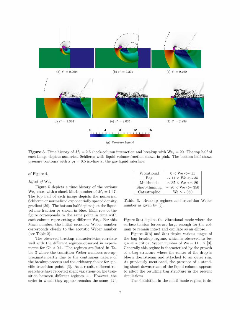
(a) t∗ = 0.099 (b) t∗ = 0.237 (c) t∗ = 0.790

(d) t∗ = 1.344 (e) t∗ = 2.035 (f) t∗ = 2.838

(g) Pressure legend

Figure 3. Time history of Ms = 2.5 shock-column interaction and breakup with Wea = 20. The top half ofeach image depicts numerical Schlieren with liquid volume fraction shown in pink. The bottom half showspressure contours with a φ1 = 0.5 iso-line at the gas-liquid interface.

of Figure 4.

Effect of Wea

Figure 5 depicts a time history of the variousWea cases with a shock Mach number of Ms = 1.47.The top half of each image depicts the numericalSchlieren or normalized exponentially spaced densitygradient [39]. The bottom half depicts just the liquidvolume fraction φ1 shown in blue. Each row of thefigure corresponds to the same point in time witheach column representing a different Wea. For thisMach number, the initial crossflow Weber numbercorresponds closely to the acoustic Weber number(see Table 2).

The observed breakup characteristics correlatewell with the different regimes observed in experi-ments for Oh < 0.1. The regimes are listed in Ta-ble 3 where the transition Weber numbers are ap-proximate partly due to the continuous nature ofthe breakup process and the arbitrary choice for spe-cific transition points [3]. As a result, different re-searchers have reported slight variations on the tran-sition between different regimes [4]. However, theorder in which they appear remains the same [42].

Vibrational 0 < We <∼ 11Bag ∼ 11 < We <∼ 35

Multimode ∼ 35 < We <∼ 80Sheet-thinning ∼ 80 < We <∼ 350Catastrophic We >∼ 350

Table 3. Breakup regimes and transition Webernumber as given by [3].

Figure 5(a) depicts the vibrational mode where thesurface tension forces are large enough for the col-umn to remain intact and oscillate as an ellipse.

Figures 5(b) and 5(c) depict various stages ofthe bag breakup regime, which is observed to be-gin at a critical Weber number of We = 11 ± 2 [3].Generally this regime is characterized by the growthof a bag structure where the center of the drop isblown downstream and attached to an outer rim.As previously mentioned, the presence of a stand-ing shock downstream of the liquid column appearsto affect the resulting bag structure in the presentsimulations.

The simulation in the multi-mode regime is de-

7

(a) t∗ = 0.556 (b) t∗ = 0.514

(c) t∗ = 1.132 (d) t∗ = 1.344

(e) t∗ = 1.898 (f) t∗ = 2.035

(g) t∗ = 2.857 (h) t∗ = 2.838

(i) Ms = 1.47 pressure legend (j) Ms = 2.5 pressure legend

Figure 4. Streamlines for the shock-column interaction with Wea = 20 for the Ms = 1.47 (left) andMs = 2.5 (right) simulations. The top half of each image depicts streamlines overlaid on numerical Schlierenwith liquid volume fraction shown in pink. The bottom half shows pressure contours with a φ1 = 0.5 iso-lineat the gas-liquid interface.

8

t∗ = 0.38

0.77

1.15

1.53

1.92

2.30

2.68

3.07

(a) Wea = 5,We = 4.7

(b) 10, 9.4 (c) 20, 19 (d) 50, 47 (e) 100, 94

Figure 5. Time history of Ms = 1.47 shock-column interaction. The number on the left side of eachimage row lists t∗ = t/tc, or the non-dimensional solution time scaled by the characteristic breakup timetc =

√εD/u computed using post shock conditions. Each image shows liquid volume fraction in blue with

the top half also showing numerical Schlieren.

9

picted in Figure 5(d). In this regime, the center ofthe column is driven downstream more slowly lead-ing to the creation of a bag/plume structure [43].This behavior appears to be exaggerated by thepresence of the standing shock previously mentionedwith a substantial plume/bag-and-stamen structureforming. Finally, the numerical Schlieren depicts in-creasing amounts of liquid mass being stripped fromthe surface of the column as the Weber numberincreases into the lower end of the sheet-thinningregime in Figure 5(e).

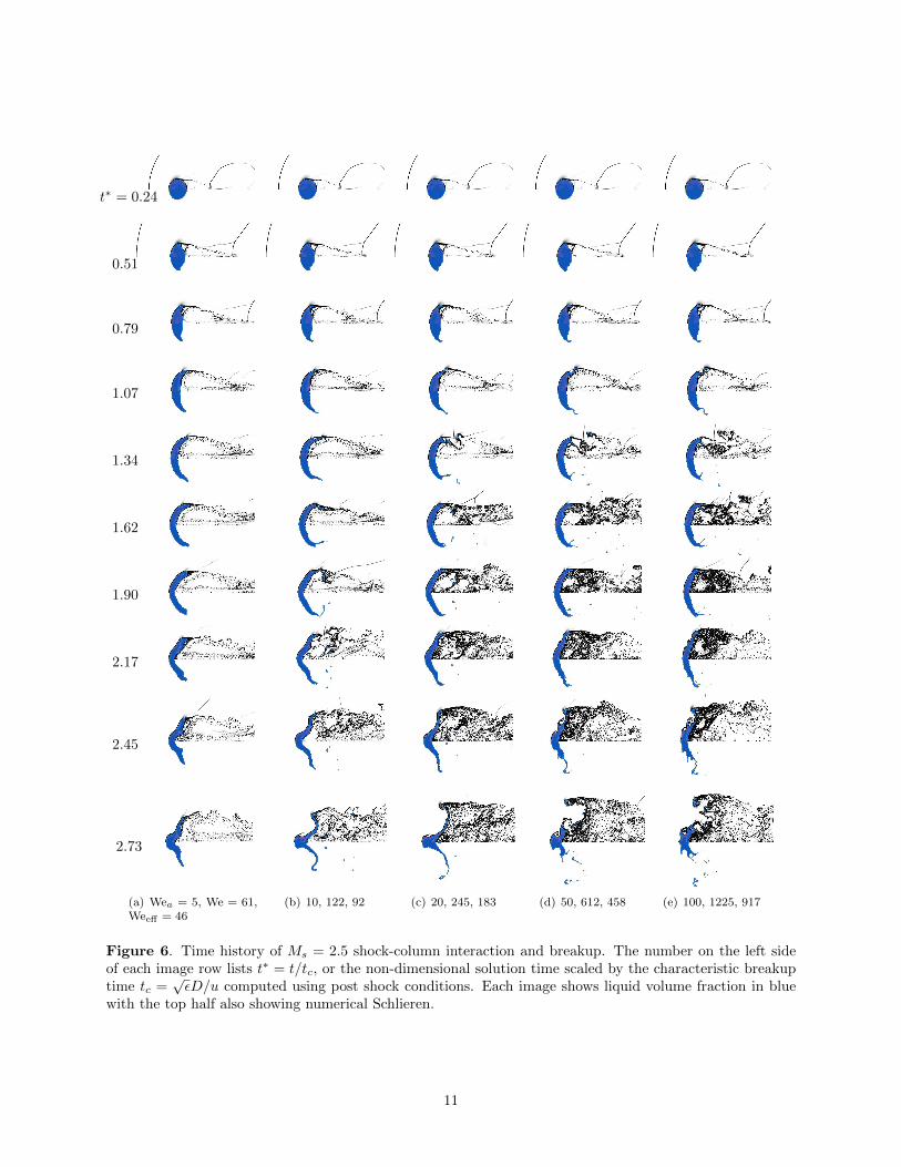
Figure 6 depicts the history of the Ms = 2.5 sim-ulations at various acoustic Weber numbers. Dueto the higher flow speeds behind the shock, theestimated initial crossflow Weber number is muchhigher for each case compared to the correspondingMs = 1.47 simulations (see Table 2).

Theofanous et al. [44] performed experiments ofaerobreakup of spherical liquid droplets in M = 3crossflows. They observed “piercing” (44 < We <103) and “stripping” (∼ 103 < We) breakup regimes.The range of breakup features depicted in Figure 6with the estimated effective Weber numbers varyingfrom 46 in Figure 6(a) to 917 in Figure 6(e) appearto qualitatively match descriptions of those regimesdespite the disparity in crossflow speeds (M = 1.2for the Ms = 2.5 case versus M = 3 in the experi-ments) and flow dimensionality.

Drag coefficient and column trajectory

Finally, the drag coefficient and trajectory ofthe liquid columns is examined. Figure 7 depictscomparisons of the early stages of the drag coeffi-cient with prior numerical results of Meng and Colo-nius [17], Chen [22], and Terashima and Tryggva-son [20]. The drag coefficient was computed follow-ing [17]:

Cd =mac

12ρg(ug − uc)2d0

(19)

where d0 is the undeformed diameter of the column,ρg and ug are the initial post-shock gas conditionsand uc is the center of mass velocity given by equa-tion 15. The acceleration is then computed usingfinite differences in time [17]:

ac =d

dt

∫ρ1φ1udV∫ρ1φ1dV

. (20)

Good agreement is obtained with the data of [17],disparities in the other results can likely be at-tributed to the use of a different approach to calcu-late the drag coefficient, where drift data (and notaveraged fluid velocity) is used to estimate the col-umn acceleration. Refer to [17] and [15] for further

discussion of different approaches for computing thedrag coefficient.

Figure 8 depicts the drag coefficient at thelater stages of the simulations with comparisons toan approximately rigid and stationary liquid col-umn computed with a high liquid density (ρl =10, 000 kg/m3) case with Wea = 5. This extrasimulation was performed to provide a referencepoint to a stationary and rigid cylinder in crossflowwhere the drag coefficient is known. Generally for100 < Re < 105, the drag coefficient of a cylinderis known to be approximately 1 which agrees wellwith the present subsonic simulation with a cross-flow Reynolds number of 1430. Meanwhile fromGowen and Perkins [45] the drag coefficient of a sta-tionary cylinder in M = 1.2 flow is approximately1.6. This agrees well with the minimum drag co-efficient value computed for the simulation of theapproximately rigid stationary cylinder which oc-curs around t∗ = 0.3 in Figure 8. Variations of thedrag coefficient in this simulation can be attributedto the gradual deformation of the high density col-umn. Gowen and Perkins also noted there was al-most no observed variation in the drag coefficientas a function of Reynolds number in the supersonicflow regime. Interestingly, the present results sug-gest for the liquid column there is significantly lessvariation in the drag coefficient as a function of theWeber number in the supersonic regime.

Overall, the drag coefficient exhibits signifi-cantly less unsteady variation compared to the re-sults of [17], however, the general trend is similar.The differences can be attributed to the inclusionof surface tension, molecular viscosity, and inter-face sharpening employed in the current simulations.Lower drag coefficients are observed with lower We-ber numbers for both shock Mach numbers. Sig-nificant differences in the drag as a function of theWeber number are observed in the Ms = 1.47 case inFigure 8(a). Consistent with the breakup behaviordescribed previously, less variation is observed be-tween the different Weber numbers in the Ms = 2.5case as depicted in Figure 8(b).

Supporting the experimental observations ofTemkin and Mehta [11], the unsteady drag is foundto be larger in the decelerating relative flows of theliquid columns compared to that of the rigid sta-tionary column. The coefficients are observed to bearound twice as large as the rigid case for both shockMach numbers at Wea = 5.

Figure 9(a) depicts the decreasing relative ve-locity of the liquid columns as a function of timewith the velocity normalized by the post-shock gasvelocity. The Ms = 1.47 case with Wea = 5 exhib-

10

t∗ = 0.24

0.51

0.79

1.07

1.34

1.62

1.90

2.17

2.45

2.73

(a) Wea = 5, We = 61,Weeff = 46

(b) 10, 122, 92 (c) 20, 245, 183 (d) 50, 612, 458 (e) 100, 1225, 917

Figure 6. Time history of Ms = 2.5 shock-column interaction and breakup. The number on the left sideof each image row lists t∗ = t/tc, or the non-dimensional solution time scaled by the characteristic breakuptime tc =

√εD/u computed using post shock conditions. Each image shows liquid volume fraction in blue

with the top half also showing numerical Schlieren.

11

0 0.02 0.04 0.06 0.08 0.1t$

0

1

2

3

4

5

6

Cd

Meng & ColoniusChenTerashima & TryggvasonWea = 100

(a) Ms = 1.47

0 0.02 0.04 0.06 0.08 0.1t$

0

0.5

1

1.5

2

2.5

3

Cd

Meng & ColoniusWea = 100

(b) Ms = 2.5

Figure 7. Drag coefficient comparison during the early stages for Ms = 1.47 (left) and Ms = 2.5 (right)compared to Meng and Colonius [17], Chen [22], and Terashima and Tryggvason [20].

0 0.5 1 1.5t$

0

1

2

3

4

5

6

7

Cd

Meng & ColoniusWea = 100Wea = 20Wea = 5;l = 10; 000 kg=m3

(a) Ms = 1.47

0 0.5 1 1.5t$

0

1

2

3

4

5

6

7

Cd

Meng & ColoniusWea = 100Wea = 20Wea = 5;l = 10; 000 kg=m3

(b) Ms = 2.5

Figure 8. Drag coefficient comparison at the later stages for Ms = 1.47 (left) and Ms = 2.5 (right) comparedto Meng and Colonius [17].

ited the lowest drag coefficient and correspondinglyshows the highest relative velocity at t∗ = 1.5. Fig-ure 9(b) shows the trajectories of the liquid massover time. Interestingly, up to t∗ = 1.5 the columntrajectories largely collapse on each other when plot-ted against the characteristic time t∗ .

Conclusion

Numerical experiments of Ms = 1.47 and Ms =2.5 shockwaves interacting with liquid columns areperformed. The effects of compressibility, molecu-lar viscosity, and surface tension are accounted for.The shockwaves induce a crossflow leading to aero-breakup of the liquid column. As the Weber num-ber is varied several breakup modes are observedwith good correlation to the experimentally observedbreakup characteristics. The Ms = 2.5 shock leads

to supersonic flow around the column. This affectsthe shape of the recirculation region behind the col-umn and is observed to affect the corresponding de-formation and breakup of the liquid. At higher We-ber numbers there is an increase in the quantity ofliquid mass stripped from the surface of the column.Lower Weber numbers resulted in lower observeddrag coefficients for the liquid columns. However,depending on the Weber number the drag coeffi-cients were still approximately two to three timesthose observed for a rigid liquid column.

Acknowledgments

This work is supported by Taitech, Inc. un-der sub-contract TS16-16-61-004 (primary contractFA8650-14-D-2316). The research reported in thispaper is partially supported by the HPC@ISU equip-

12

0 0.5 1 1.5t$

0.8

0.85

0.9

0.95

1

(ug!

uc)=

ug

Ms = 1:47, Wea = 100Ms = 1:47, Wea = 5Ms = 2:5, Wea = 100Ms = 2:50, Wea = 5

(a) Velocity

0 0.5 1 1.5t$

0

0.5

1

1.5

2

xc=D

Ms = 1:47, Wea = 100Ms = 1:47, Wea = 5Ms = 2:5, Wea = 100Ms = 2:50, Wea = 5

(b) Position

Figure 9. Column center of mass velocity (a) and position (b) as a function of t∗.

ment at Iowa State University, some of which hasbeen purchased through funding provided by NSFunder MRI grant number CNS 1229081 and CRIgrant number 1205413.

References

[1] Mikhael Gorokhovski and Marcus Herrmann.Annual Review of Fluid Mechanics, 40:343–366,2008.

[2] Jinho Lee, Kuo-Cheng Lin, and Dean Eklund.AIAA Journal, 53(6):1405–1423, 2015.

[3] D. R. Guildenbecher, C. Lopez-Rivera, andP. E. Sojka. Experiments in Fluids, 46(3):371–402, 2009.

[4] M. Pilch and C. A. Erdman. InternationalJournal of Multiphase Flow, 13(6):741–757,1987.

[5] L. P. Hsiang and G. M. Faeth. Interna-tional Journal of Multiphase Flow, 18(5):635–652, 1992.

[6] G. M. Faeth, L. P. Hsiang, and P. K.Wu. International Journal of Multiphase Flow,21(Suppl):99–127, 1995.

[7] K. S. Im, K. C. Lin, M. C. Lai, and M. S. Chon.International Journal of Automotive Technol-ogy, 12(4):389–496, 2011.

[8] H. Liu, Y. Guo, and W. Lin. Advances in Me-chanical Engineering, 8(1):1–13, 2016.

[9] Clayton T Crowe, John D Schwarzkopf, Mar-tin Sommerfeld, and Yutaka Tsuji. Multiphaseflows with droplets and particles. CRC Press,2011.

[10] Inchul Kim, Said Elghobashi, and William A.Sirignano. Journal of Fluid Mechanics,367(1998):221–253, 1998.

[11] S Temkin and H K Mehta. Journal of FluidMechanics, 116:297–313, 1982.

[12] Amrita Wadhwa, Vinicio Magi, and John Abra-ham. Physics of Fluids, 19(11), 2007.

[13] D. Igra and K. Takayama. Atomization andSprays, 11:167–185, 2001.

[14] S. Sembian, M. Liverts, N. Tillmark, andN. Apazidis. Physics of Fluids, 28(5), 2016.

[15] D. Igra, T. Ogawa, and K. Takayama. Atom-ization and Sprays, 12:577–591, 2002.

[16] D Igra and M Sun. AIAA Journal, 48(12):2763–2771, 2010.

[17] J. C. Meng and T. Colonius. Shock Waves, pp.399–414, 2014.

[18] Ratnesh K. Shukla, Carlos Pantano, andJonathan B. Freund. Journal of ComputationalPhysics, 229(19):7411–7439, 2010.

[19] Ratnesh K. Shukla. Journal of ComputationalPhysics, 276:508–540, 2014.

[20] Hiroshi Terashima and Gretar Tryggva-son. Journal of Computational Physics,228(11):4012–4037, 2009.

[21] Hiroshi Terashima and Gretar Tryggvason.Computers and Fluids, 39:1804–1814, 2010.

[22] H. Chen. AIAA Journal, 46(5):1135–1143,2008.

13

[23] Taku Nonomura, Keiichi Kitamura, and KozoFujii. Journal of Computational Physics,258:95–117, 2014.

[24] Daniel P Garrick, Mark Owkes, andJonathan D Regele. Journal of Computa-tional Physics, In Press, 2017.

[25] Daniel P Garrick, Wyatt A Hagen, andJonathan D Regele. Submitted to Journal ofComputational Physics, 2017.

[26] Gregoire Allaire, Sebastien Clerc, and SamuelKokh. Journal of Computational Physics,181(2):577–616, 2002.

[27] Guillaume Perigaud and Richard Saurel. Jour-nal of Computational Physics, 209(1):139–178,2005.

[28] J. U. Brackbill, D.B. Kothe, and C. Zemach.Journal of Computational Physics, 100:335–354, 1992.

[29] Denis Gueyffier, Jie Li, Ali Nadim, Ruben Scar-dovelli, and Stephane Zaleski. Journal of Com-putational Physics, 152(2):423–456, 1999.

[30] F Harlow and A Amsden. Fluid Dynamics,Technical Report LA-4700, Los Alamos Na-tional Laboratory, Los Alamos, NM, 1971.

[31] Vedran Coralic and Tim Colonius. Journal ofComputational Physics, 274:95–121, 2014.

[32] E F Toro, M Spruce, and W Speares. ShockWaves, 4(1):25–34, 1994.

[33] Eleuterio F Toro. Riemann Solvers and Numer-ical Methods for Fluid Dynamics: A PracticalIntroduction. Springer, New York, 2009.

[34] Eric Johnsen and Tim Colonius. Journal ofComputational Physics, 219(2):715–732, 2006.

[35] Sigal Gottlieb and Chi-Wang Shu. Mathematicsof Computation, 67(221):73–85, 1998.

[36] Hong Luo, Joseph D. Baum, and RainaldLohner. Journal of Computational Physics,194(1):304–328, 2004.

[37] F. Xiao, Z. G. Wang, M. B. Sun, J. H. Liang,and N. Liu. International Journal of MultiphaseFlow, 87:229–240, 2016.

[38] J. A. Nicholls and A. A. Ranger. AIAA Journal,7(2):285–290, 1969.

[39] James J Quirk and Smadar Karni. NASA Con-tractor Report 194978, 1994.

[40] J. Han and G. Tryggvason. Physics of Fluids,11(12):3650, 1999.

[41] J. Han and G. Tryggvason. Physics of Fluids,13(6):1554–1565, 2001.

[42] M. Jain, R. S. Prakash, G. Tomar, and R. V.Ravikrishna. Proceedings of the Royal Soci-ety A: Mathematical, Physical and EngineeringSciences, 471(2177):20140930–20140930, 2015.

[43] Z Dai and G M Faeth. International Journal ofMultiphase Flow, 27:217–236, 2001.

[44] T. G. Theofanous, G. J. Li, and T. N. Dinh.Journal of Fluids Engineering, 126(4):516,2004.

[45] Forrest E. Gowen and Edward W. Perkins.NACA Technical Note 2960, 1953.

14