DPRIETI Discussion Paper Series 08-E-013

Does Trade Liberalization Reduce Pollution Emissions?

MANAGI ShunsukeYokohama National University

HIBIKI AkiraNational Institute for Environmental Studies, Japan

TSURUMI TetsuyaYokohama National University

The Research Institute of Economy, Trade and Industryhttp://www.rieti.go.jp/en/

RIETI Discussion Paper Series 08-E-013

Does Trade Liberalization Reduce Pollution Emissions?

Shunsuke Managi1*, Akira Hibiki2 and Tetsuya Tsurumi1

1 Faculty of Business Administration, Yokohama National University 79-4, Tokiwadai, Hodogaya-ku, Yokohama 240-8501 Japan

Tel. 81- 45-339-3751/ Fax: 81- 45-339-3707 *Corresponding author (managi@ynu.ac.jp)

2 Social Environmental Systems Division, National Institute for Environmental Studies, Japan

RHH: MANAGI, HIBIKI & TSURUMI: TRADE AND ENVIRONMENT

*** Note: This is a revised version that replaces the original paper published May 2008***

Abstract

The literature on trade openness, economic development, and the environment is largely inconclusive about the environmental consequences of trade. This study treats trade and income as endogenous and estimates the overall impact of trade openness on environmental quality using the instrumental variables technique. We find the impact is large in the long term, after the dynamic adjustment process, although it is small in the short term. Trade is found to benefit the environment in OECD countries. It has detrimental effects, however, on sulfur dioxide (SO2) and carbon dioxide (CO2) emissions in non-OECD countries, although it does lower biochemical oxygen demand (BOD) emissions in these countries. Finally, trade openness influences emissions through the environmental regulation effect and capital labor effect. We find that the former effect is likely to be larger than the latter effect for all pollutants.

JEL. F18; O13; L60; L50

Keywords: Trade Openness; Composition Effect; Scale Effect, Technique Effect;

Environment; Comparative Advantage; Environmental Regulations Effect.

1

1. Introduction

The environmental effect of trade openness has been one of the most important

questions in trade policy for the past 10 years (see Copeland and Taylor, 2005; Taylor,

2004). Empirical studies on the relationship between international trade openness and

environmental quality have been accumulating (see, e.g., Antweiler et al., 2001;

Harbaugh et al., 2002; Cole and Elliott, 2003; Frankel and Rose, 2005). However, there

are very few empirical studies on the determinants of emissions based on the theoretical

framework.

Antweiler et al. (2001) first provide the theoretical framework to empirically

explore the determinants of emissions and to successfully decompose them into scale,

technique, and composition effects. The scale effect refers to the effect of an increase in

production (e.g., GDP) on emissions. The technique effect indicates the negative impact

of income on emission intensity. This refers to the effect of more stringent

environmental regulations, which promote the employment of more

environmentally-friendly production methods and which are put in place as additional

income increases the demand for a better environment. The composition effect explains

how emissions are affected by the composition of output (i.e., the structure of the

industry), which is determined by the degree of trade openness as well as by the

comparative advantage of the country. This effect could be positive or negative,

depending on the country’s resource abundance and the strength of its environmental

policy. These are called the capital–labor effect (KLE) and the environmental regulation

effect (ERE), respectively1. 1 Countries where the capital-labor ratio is relatively high are expected to have a comparative

advantage in capital-intensive goods (i.e., pollution goods) and thus, to produce more emissions.

Trade openness would strengthen the effects of this comparative advantage and of any

2

Since trade openness could increase production and income, it affects emissions

through the scale effect and the technique effect (Antweiler et al., 2001). Hereafter, we

call these effects the trade-induced scale effect and the trade-induced technique effect.

Antweiler et al. (2001) estimate how trade openness (increase in trade intensity) and

GDP (or per capita income) affect pollution by using data on sulfur dioxide (SO2)

concentrations. They find that SO2 concentrations increase as GDP rises (i.e., positive

scale effect), decrease as per capita income rises (i.e., negative technique effect), and

decrease as trade openness rises (i.e., negative composition effect). Similarly, Cole and

Elliott (2003) analyze country-level emissions per capita of sulfur dioxide (SO2), carbon

dioxide (CO2), nitrogen oxides (NOx), and biochemical oxygen demand (BOD)) and

estimate the net of the scale effect and the technique effect, and the composition effect2.

between-country differences in environmental policy on the industrial structure. Therefore, more

openness would increase the production share of the goods in which these countries have a

comparative advantage (i.e., capital-intensive goods). On the other hand, trade openness would

reduce the comparative advantage of capital-intensive goods in countries that have relatively strict

environmental policies (i.e., higher income countries) while increasing the comparative advantage of

such goods in countries with less stringent environmental regulations (i.e., laxity is a source of

comparative advantage). As a result, the production of capital-intensive goods under more (or less)

stringent regulations decreases (increases), and the emissions decrease (increase). This is called the

ERE, or, in other words, the pollution haven effect. The net effect of the composition effect as a

result of trade openness could therefore be positive or negative, depending on the relative sizes of

the KLE and the ERE (see Cole and Elliott, 2003). 2 In Cole and Elliott (2003, 2006), the scale effect and the technique effect are not separated because

real GDP per capita is used as a proxy for both production and per capita income level. Therefore,

the net of the scale effect and the technique effect is estimated and named the scale-technique effect.

In this study, we estimate the scale-technique effect following Cole and Elliott (2003, 2006). Hence,

we call the net of the trade-induced scale effect and the trade-induced technique effect as the

trade-induced scale-technique effect.

3

However, these previous studies do not consider the endogeneity problem and,

therefore, do not treat the effect of trade openness on production or income explicitly.

Therefore, the effects of trade openness on emissions via income and production

changes (i.e., the trade-induced scale and technique effects) cannot be compared to the

composition effect induced by trade. As a result, we cannot infer the overall

environmental consequences of trade as a summation of these effects. For instance, in

the case of Cole and Elliott’s (2003) finding on SO2 emissions, in which an increase in

income reduces emissions (i.e., negative net scale and technique effects) while trade

openness increases emissions (i.e., positive composition effects), we are not able to

judge whether the overall sign of the effect of trade on emissions is positive or negative.

Furthermore, we need to note that an increase in income (or production)

associated with trade openness might affect the composition effect. For example, the

composition effect resulting from the ERE might be larger under more stringent policies.

However, since the endogeneity of income is not considered in these previous studies,

estimates of the composition effect induced by trade do not include this effect.

We also apply a dynamic model to consider an adjustment process. This is

because it is important to clarify the short- and long-term effects of trade on the

environment. Since the former studies do not consider the dynamic adjustment process,

we must consider their results primarily to be short-term effects. This may explain why

the effects of trade on the environment that they calculate are rather small.

In this study, we explore the short-term and the long-term overall effects of trade

openness on emissions as well as decomposed effects, such as the trade-induced

scale-technique effects and the trade-induced composition effects by extending the

previous studies in the following ways: (1) we add the income equation to consider the

4

effect of trade openness on real GDP per capita explicitly, and (2) we employ a dynamic

model.

2. Model

2.1 Empirical Strategy

Antweiler et al. (2001) analyze SO2 concentrations in 43 countries from 1971 to

1996. They find positive scale effects, negative technique effects, and negative

trade-induced composition effects. Thus, since the technique effects dominate the scale

effects on average, they conclude that trade openness is associated with reduced

pollution. Similarly, Cole and Elliott (2003) and Cole (2006) analyze country-level

emissions (SO2, CO2, NOx, and BOD) and energy consumption per capita, and they

estimate the scale-technique effects and composition effects. Their findings generally

support those of Antweiler et al. (2001) for SO2. The results suggest that greater

openness reduces BOD emissions per capita but is likely to increase NOx and CO2

emissions and energy use.

These studies analyze how trade openness and income affect the environment.

However, we are not able to find a causal relationship if we treat trade openness as

exogenous3. Therefore, in addition to addressing the endogeneity of income, the

endogeneity of trade needs to be modeled to analyze the consequences of trade for the

environment (Copeland and Taylor, 2005; Frankel and Rose, 2005).

Frankel and Rose (2005) consider trade openness and income endogenously.

They address the potential simultaneity of trade, environmental quality, and income by

3 See Frankel and Romer (1999) and Noguer and Siscart (2005) for recent studies that treat trade as

endogenous and that estimate the impact of trade on income using instrumental variables.

5

applying instrumental variables estimations using a gravity model of bilateral trade and

endogenous growth from neoclassical growth equations. It should be noted that they do

not derive these estimations from a theoretical model like Antweiler et al. (2001) and

thus that they do not consider the decomposed effects. They estimate an environmental

quality equation, a trade equation, and an income equation to test a causal relationship

between trade and environmental outcomes. Using cross section data from 41 countries

in 1990 and looking at the sign of the openness variable, they support the optimistic

view that trade reduces sulfur dioxide emissions4.

In this study, we use a larger and more globally representative sample,

especially including more developing countries, of many local and global emissions

than are reflected in previous studies. Panel data used in this study are the SO2 and CO2

emissions of 88 countries from 1973 to 2000 and the BOD emissions of 83 countries

from 1980 to 2000.

In econometric models, serial correlation must be considered because the

environmental and output dependent variables have relatively monotonic trends.

However, previous studies of international trade and the environment do not control for

this factor when analyzing panel data. It should be noted that a dynamic generalized

method of moments (GMM) estimation of panel data applied to a dynamic model is

useful both to correct for serial correlation and to analyze both short- and long-term

effects of trade openness on the environment.

4 Some of the variables used in Frankel and Rose (2005) are excluded from our estimated results in

this paper because they are not statistically significant or because we are not able to explain the

intuition behind the results regarding those variables. Instead, we follow the choice of variables from

Cole and Elliott (2003). See also Chintrakarn and Millimet (2006) for another application where they

analyze the causal effect of domestic state-level trade flows on toxic emissions in the US.

6

Improving the previous studies in several ways can produce a broader view of

environmental consequences, and, therefore, we might come to different conclusions

about the linkage between international trade and environmental quality.

2.2 Model

This study considers the endogeneity of trade openness and income and then

estimates an environmental quality equation. Here, we only discuss the environmental

quality equation. Equations of income and trade openness are discussed in Appendix A.

2.2.1 Environmental Quality Equation

This study employs a specification similar to that of Cole and Elliott (2003)

under which the determinants of emissions can be decomposed into scale-technique and

composition effects. Contrary to the study by Cole and Elliott (2003), a lagged term of

the dependent variable and international protocol dummies are included. The lagged

variable is intended to control for the effect of the dynamic process.

itititititititititit

ititititit

itititititititit

OHTRSLRKTRSTRS

TLRKTLRKT

SLKLKLKSSEcE

11413122

1110

2987

62

542

32111

)/(

)/()/(

)/()/()/(lnln

εααααα

ααα

αααααα

+++⋅⋅++⋅+

+⋅++

⋅++++++= −

1 1 1it i itε η ν= + , (1)

where Eit denotes emissions (SO2, CO2, and BOD) per capita of country i in year t (for

example, kilograms of sulfur dioxide per capita), and S is GDP per capita. GDP per

capita and its quadratic are intended to capture the scale-technique effect. T is defined as

the ratio of aggregate exports and imports to GDP, which, as in the growth literature,

proxies trade openness (or trade intensity) (see, e.g., Antweiler et al., 2001; Frankel and

Rose, 2005) 5; K/L denotes a country’s capital–labor ratio; RK/L denotes a country’s 5 This study focuses on trade exposure rather than trade liberalization. See Ederington et al. (2004)

for the direct impact of liberalization on polluting activities. They study the effect of reductions in

7

relative capital–labor ratio; RS is relative GDP per capita6; and 1ε is an error term and

consists of an individual country effect 1η and a random disturbance 1ν . To address

the dynamics, the lagged dependent variable is included in (1) (see Arellano and Bond,

1991).

We are able to interpret each term following Antweiler et al. (2001) and Cole

and Elliott (2003). The third term, itS , and the fourth term, 2itS , on the right hand side

in (1) reflect the effects of income and production on emissions. From this, we expect to

estimate the scale-technique effect (Cole and Elliott, 2003). The 14th and 15th terms are

additional technique effects. These terms represent international environmental treaties

for emission reductions. In the case of SO2, two international environmental treaties are

included in the regression. H denotes the Helsinki dummy, where 1 indicates that the

country has ratified the Helsinki Protocol and 0 indicates otherwise, and O denotes the

Oslo dummy, where 1 indicates ratification of the Oslo Protocol and 0 indicates

otherwise7. We should note that the decision of a country to ratify these protocols cannot

be treated as exogenous because this decision is likely to be affected by that country’s

economic conditions (see Beron et al., 2003; Murdoch et al., 2003). Similarly, the

Kyoto Protocol and the Protocol on Water and Health are considered for the cases of

CO2 and BOD, respectively, where detailed explanations are provided later. Therefore,

to address self-selection bias, the predicted probability of reaching the ratification stage

US tariffs schedules on the output of pollution intensive industries. 6 To show a country’s comparative advantage, a country’s capital–labor ratio and per capita income

levels are expressed relative to the world average for each year, following Cole and Elliott (2003). 7 The 1985 Helsinki Protocol on the reduction of sulfur emissions and their trans-boundary fluxes

by at least 30 percent entered into force in 1987. The 1994 Oslo Protocol on the further reduction of

sulfur emissions is a successor to the Helsinki Protocol and entered into force in 1998.

8

is calculated using probit estimation and is used for these dummy variables for the

countries participating in the negotiations of these treaties8.

The fifth to 13th terms on the right hand side show the composition effects. A

country’s comparative advantage is a major factor influencing the composition effects.

We consider factor endowment, stringency of environmental regulations, and trade

openness as factors affecting the comparative advantage (as in Antweiler et al., 2000;

Cole and Elliott, 2003). A capital-abundant country will specialize in capital-intensive

production, whereas a labor-abundant country has a comparative advantage in

labor-intensive goods. Therefore, a country with a higher capital-labor ratio tends to

have higher emissions because capital-intensive goods are associated with higher

emissions (see Cole and Elliott, 2003). This effect is captured by the fifth to seventh and

ninth to 13th terms.

At the same time, however, a country with relatively more stringent regulations

has a smaller comparative advantage in capital (pollution) intensive goods because

production would be constrained by these regulations. It is important to know that there

is a strong correlation between a sector’s capital intensity and its pollution intensity (see

Cole and Elliott, 2003). Therefore, even if countries have a comparative advantage in

capital (pollution) intensive goods (i.e., a higher capital-labor ratio), the comparative

advantage is weakened and emissions would decrease in high-income countries. The

seventh term in the equation reflects this effect.

In addition, an increase in trade encourages an increase in the production of

capital-intensive goods in countries that have a comparative advantage in these goods

8 The predicted probabilities are controlled for SO2 and CO2. The value for BOD emissions is not

controlled because we are not able to obtain statistically significant results in the probit estimation.

9

and a decrease in the production of capital-intensive goods in countries that have a

comparative disadvantage in capital-intensive goods (see the explanation of the KLE in

footnote 1). This is captured by the ninth and tenth terms. An increase in trade might,

however, encourage a shift in the production of capital-intensive goods from countries

with more stringent environmental regulations (high income countries) to countries with

less stringent environmental regulation (low income countries). This effect (see the

explanation of the ERE in footnote 1) is captured by the 11th to 13th terms.

2.2.2 Income Equation

Following the endogenous growth literature (see, e.g., Mankiw et al., 1992;

Frankel and Romer, 1999), we control for trade openness, capital–labor ratio,

population, and human capital in the income equation. The income equation is:

2 1 1 2 3 4 1 5 2ln ln ln ln( / ) ln lnit it it it it it itS c S T K L P Schβ β β β β ε− −= + + + + + +

2 2 2it i itε η ν= + . (2)

where P is the population, Sch proxies human capital investment based on school

attendance years, and 2ε is an error term and consists of an individual country effect

2η and a random disturbance 2ν . The other variables have been defined previously.

2.2.3 Short-Term and Long-Term Effects and Trade-Induced Elasticity

Short-Term Effect

We can decompose the terms in equation (1) into two groups as follows. One is

the scale-technique effect ( itY ) and the other is the composition effect ( itC )9.

9 Although discussions based on the decomposition are provided, we note that the decomposed

effects are imputed instead of observed. For example, one could consider the case in which a higher

K/L also leads to higher energy inputs, and there may not be compositional effects. Hence K/L may

capture a technique effect, as S does. Similarly, a higher S may also induce structural shifts due to

non-homothetic demand (see Echevarria, 2008) that move demand to cleaner service–type sectors.

10

[ ] ititititit OHSSY 14132

32 αααα +++= (3)

[ ][ ] [ ] itititititititititititit

ititititit

TRSLRKTRSTRSTLRKTLRKT

SLKLKLKC

⋅⋅++⋅++⋅++

⋅++=

)/()/()/(

)/()/()/(

122

11102

987

62

54

αααααα

ααα

(4)

Equation 4 is divided into two parts: one with terms including itT , which

captures the effect of trade openness on the composition effect through the factor

endowment and/or the environmental regulation effect, and another one without terms

including itT .

The first part of equation 4 is the direct effect of trade, and the latter is the

indirect effect of trade. We name the former the Direct Trade-Induced Composition

Effect ( itTC ) and the latter the Indirect Trade-Induced Composition Effect ( itOC ). This

reflects the indirect effect of a trade-induced change in income on emissions. Once the

environmental regulations in a country become more stringent following an increase in

income, that country loses its comparative advantage in capital-intensive goods. Thus,

TCit and OCit are expressed as follows:

[ ][ ] ititititititit

itititititit

TRSLRKTRSTRS

TLRKTLRKTTC

⋅⋅++⋅+

+⋅+=

)/(

)/()/(

122

1110

2987

ααα

ααα (5)

[ ] ititititit SLKLKLKOC ⋅++= )/()/()/( 62

54 ααα (6)

Here, we consider the effect of a one- percent increase in trade intensity. SSTσ 10

is the trade elasticity of emissions driven by the scale-technique effect through changes

in income. It is derived from (1) and given in (7). In the same way, STCσ is the trade

Hence, S may have little relationship with regulation at all but may have a compositional effect. 10 The superscripts “S” and “L” refer to the short- and long-term effects, respectively.

11

elasticity of emissions driven by the direct composition effect. It is derived from (5) and

given in (8). Finally, SOCσ 11 is the trade elasticity of emissions driven by the indirect

composition effect through changes in income. It is derived from (6) and given in (9). It

should be noted that we use the short-term trade elasticity of income, which is

calculated from the income equation as β2, to obtain these elasticities.

( ) ititSST SS 232 2 βαασ += (7)

( )

[ ] [ ]( )10 11 12 2

2 27 8 9 10 11 12

2 ( / )

( / ) ( / ) ( / )

STC it i it

it it it it it it it

RS RK L RS

RK L RK L RS RS RK L RS T

σ α α α β

α α α α α α

= + +⎡⎣⎤+ + + + + + ⋅⎦

(8)

( ) ititSOC SLK 26 )/( βασ = (9)

As we can see from equation (5), the effect of an increase in trade intensity on

emissions in (8) is divided into two effects: the direct effect of trade intensity and the

indirect effect of trade intensity through changes in income. We define SITCσ 12 and

SDTCσ 13 as the elasticities that represent both of these effects.

( ) ititiitSITC TRSLRKRS 2121110 )/(2 βααασ ++= (10)

[ ] [ ]( )2 27 8 9 10 11 12( / ) ( / ) ( / )S

DTC it it it it it it itRK L RK L RS RS RK L RS Tσ α α α α α α= + + + + + ⋅

(11)

11 This elasticity implies an indirect trade-induced composition effect, or, more precisely, a

composition effect caused by trade-induced income changes that affect the stringency of the

country’s environmental regulations and that result in a change in the comparative advantage of

capital-intensive goods. 12 This is an indirect trade-induced composition effect. It is caused by a trade-induced income

change that affects the ERE or the KLE. 13 This is a direct trade-induced composition effect. It is caused by a trade intensity change that

affects the ERE or the KLE.

12

From these elasticities, the total trade-induced composition effect, SCσ , is calculated as

SITC

SDTC

SOC

SC σσσσ ++= . However, the total trade-induced composition effect used by

Cole and Elliott (2003) corresponds to SDTCσ . Hence, they ignore the influence of S

OCσ

and SITCσ . This might overestimate or underestimate the composition effect. Finally, the

short-term overall trade openness elasticity of emissions, STσ , is calculated as follows:

S S S S ST ST OC ITC DTCσ σ σ σ σ= + + + (12)

Long-Term Effect

In the same manner, each of the long-term effects of LSTσ , L

OCσ , LTCσ , L

ITCσ ,

and LDTCσ can be defined. Considering that the long-term elasticity of trade openness to

income is calculated as 2 1(1 )β β− , these effects are calculated as follows:

( ) iiLST SS

11

232 1

11

2αβ

βαασ

−−+= (13)

( ) iiLOC SLK

11

26 1

11

)/(αβ

βασ

−−= (14)

( )

[ ] [ ]( )

210 11 12

1

2 27 8 9 10 11 12

1

2 ( / )1

1( / ) ( / ) ( / )1

LTC i i i

i i i i i i i

RS RK L RS

RK L RK L RS RS RK L RS T

βσ α α αβ

α α α α α αα

⎡= + +⎢ −⎣

⎤+ + + + + + ⋅⎦ −

(15)

( ) iiiiLITC TRSLRKRS

11

2121110 1

11

)/(2αβ

βααασ−−

++= (16)

[ ] [ ]( ) iiiiiiiLDTC TRSLRKRSRSLRKLRK

112

21110

2987 1

1)/()/()/(α

αααααασ−

⋅+++++=

(17)

The long-term overall trade openness elasticity of emissions, LCσ , is calculated as

follows:

13

L L L L LT ST OC ITC DTCσ σ σ σ σ= + + + (18)

3. Estimation Strategy and Data

3.1 Differenced GMM

Perman and Stern (2003) use the same data source for SO2 emissions as we do,

and they find that a co-integrating relation exists between SO2 emissions per capita,

income, and income squared for each country. This implies that long-run relationships

exist among these variables and that the process of adjustment to the long-run

equilibrium is slow. Since there is a possibility that other variables in our data also have

long-run relationships, it is appropriate to adopt a model that takes the time factor into

consideration in our study.

To address the dynamics, we adopt a differenced GMM, which is proposed by

Arellano and Bond (1991). This method has the advantage that it controls for both the

long-run relationship and any endogeneity problems by including appropriate

instrumental variables. We include dependent variables before t-2 and predicted values

of both trade openness and income as instrumental variables.

3.2 Data

The data used in this study are obtained from different sources. We obtain SO2

emissions data from The Center for Air Pollution Impact and Trend Analysis (CAPITA)

and Stern (2005). This data set is superior to other data sets in terms of its spatial and

temporal resolution and extent (Stern, 2005), and it covers more time and countries than

the data Cole and Elliot applied. We also obtained updated CO2 emissions data and

BOD emissions data from the same source as Cole and Elliot (2003); these data are

beneficial for drawing comparisons with Cole and Elliot. The CO2 data is obtained from

14

the Carbon Dioxide Information Analysis Center (CDIAC), and the BOD data is

obtained from World Development Indicators (WDI).

As discussed in Cole and Elliot (2003), because emissions data are often

estimated using engineering functions based on inputs, the engineering assumptions

may not reflect the true gains from techniques precisely14. However, our estimates are

able to adequately capture technique effects since each of these estimates considers

country and year specific information. For example, in the case of SO2, the sulfur

release factor is determined by technology information obtained by country and year

from the International Energy Agency. This information is combined with the sulfur

content data for refined products and the net production and is used in the final emission

calculations (Lefohn et al., 1999). The data for CO2 is calculated using CO2 emissions

factors for individual fuels, which stem from country and year specific estimates of fuel

use. Since CO2 emissions factors cannot be reduced by end-of-pipe technology, they are

time-invariant. However, regulations and technology improve fuel efficiency. Therefore,

these emissions factors are generally updated over time to allow for changes in

technology and regulations (Marland et al., 2000). On the other hand, the BOD

emissions data is based on each country’s actual monitoring data, which measures the

amount of oxygen that bacteria in water consume in breaking down waste15. Hettige et

al. (1998) first apply this data. They note that water pollution data are relatively reliable

because the sampling techniques for measuring water pollution are more widely

understood and much less expensive than those for air pollution. The World Bank’s

14 On the other hand, concentrations data tend to be affected by site-specific factors. For example,

SO2 gas is produced from not only anthropogenic sources such as the burning of fossil fuels but also

from natural sources such as transboundary movement and volcanoes. 15 This is a standard water-treatment test for the presence of organic pollutants.

15

Development Research Group updated the data through 2004 using the same

methodology as Hettige et al. (1998).

SO2 and BOD have local and trans-boundary impacts, whereas CO2 is a

greenhouse gas and has a global impact. See Cole and Elliot (2003) for a more detailed

comparison of each emission. For data on SO2 and CO2, we have observations for 88

countries covering the period from 1973–2000. For data on BOD, we have observations

for 83 countries for the period from 1980–200016. We are able to obtain large sample

sizes because annual data and data for a longer time span are available from several

different data sources. For example, in case of SO2, our SO2 emissions data is annual

and covers many countries, while Cole and Elliot (2003) obtain 5-year data from the

United Nations Environment Programme: Environmental Data Report 1993-1994,

which covers fewer countries.

Per capita income, which is defined as GDP per capita (measured in real

dollars), and trade openness are taken from the Penn World Table 6.1. The capital-labor

ratio is obtained from the Extended Penn World Table. Population and land area data

come from the WDI. Data on school attainment (years) come from the education data

set in Barro and Lee (2000), and distances between the country pairs in question

(physical distance and dummy variables indicating common borders, linguistic links,

and landlocked status) come from the Center for International Prospective Studies.

16 A list of countries used in this study for SO2, CO2, and BOD is presented in Appendix C.

16

4. Estimation Results

4.1. Parameter Estimates

Table 1 presents the results of the differenced GMM with instrumental variables

estimation of the environmental quality equation for SO2, CO2, and BOD.17 Before

discussing the result, it should be noted that the estimation methodology (i.e., the

differenced GMM estimation taking endogeneity into account) is found to be more

important to our results than the data used (see Appendix F for detail). In other words,

the differences between the results of Antweiler et al. (2001) and Cole and Elliot (2003)

and our results seem mainly to stem from estimation methods rather than from data18. In

the equations, the Sargan test for over-identifying restrictions and the hypothesis of no

second-order autocorrelation imply that the instruments used in the GMM estimation

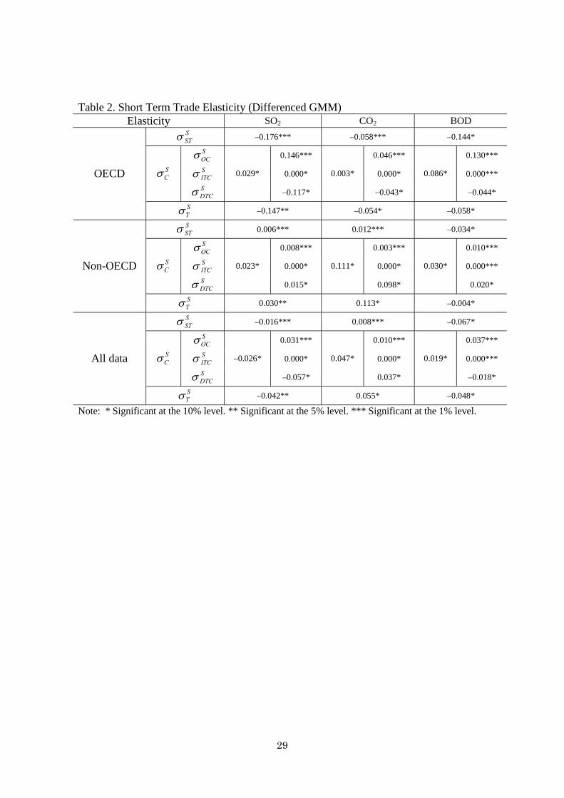
are valid and that there is no serial correlation in the error term19. Table 2 and Table 3

report the short-term and long-term elasticities of trade openness on emissions, STσ ,

Cσ , OCσ , ITCσ , DTCσ and Tσ , respectively. They are evaluated for sample averages

of OECD countries and non-OECD countries using the estimated parameters. The

values calculated with an average of all samples are also reported for reference. We

obtained statistically significant results for all elasticities.

The lagged emissions terms for all specifications are statistically significant with

a positive sign, but their values are less than one. These results imply that changes in

17 For a robustness check, Appendix D provides results for different estimation techniques. The

results for NOx are provided in Appendix E. 18 The differences in estimation results between our study and the previous studies might be caused

by changes in data and/or by differences in estimation methods. We intend to identify the sources of

such differences. The identifications of discrepancies between our study and former studies are

provided in Appendix F, which includes replications of Cole and Elliot (2003). 19 In the case of BOD, we are not able to pass AR(2) tests, though the t-value is small enough.

17

explanatory variables, such as trade openness, at a specific point in time would also

influence emissions after the current period. This indicates that there is an adjustment

process and that the short- and long-term effects of trade on emissions are different.

Therefore, we need to use a dynamic model, although previous studies do not.

Comparing Table 2 to Table 3, we find that the long-term elasticities are larger than the

short-term elasticities.

In all of the specifications for SO2, CO2, and BOD, almost all of the variables,

including the endogenous variables such as trade openness, per capita income, and their

interaction terms, have statistically significant effects. It is important to note that our

statistical results for SO2, CO2, and BOD are somewhat different from those of Cole and

Elliott (2003). As is discussed in Appendix D, these discrepancies are caused by

differences in the estimation methods. In the methods, we correct for serial correlation,

use dynamic GMM, and use instrumental variables techniques.

The sign of S is positive with statistical significance in the SO2 and CO2

estimates but negative in the BOD estimates, while the sign of S2 is negative with

statistical significance in all three estimates. These results indicate that (i) the

scale-technique effect is negative for BOD and (ii) a negative technique effect gradually

dominates a positive scale effect for SO2 and CO2 as income increases because higher

income leads to a greater demand for a better environment. To consider the effect of an

increase of S on per capita SO2, CO2 and BOD emissions more precisely, we calculated

the values of 2 32 Sα α+ and STσ using sample means of income in OECD and

non-OECD countries. We find that both values are negative for SO2 and CO2 in OECD

countries but positive in non-OECD countries20. In other words, an increase in either 20 2β is estimated to be statistically significant with a positive sign, as is discussed in Appendix A.

18

production or income leads to an increase in emissions in non-OECD countries but to a

decrease in emissions in OECD countries. Thus, in the average non-OECD country, the

scale effect dominates the technique effect because of the overall lower demand for a

better environment due to lower income, whereas in the average OECD country the

technique effect dominates the scale effect.

We also find that both the average OECD country and the average non-OECD

country have a negative value for BOD. Hence, the technique effect dominates the scale

effect in both developed and developing countries. This might be because the social

pressure against water pollution is likely to be stronger than that against air pollution. In

addition, there is some evidence that developing countries use abatement technologies

for SO2 from developed countries less frequently than those for BOD, possibly because

of higher costs (Cheremisinoff, 2001). Thus, a technique effect might be more likely to

dominate a scale effect in the case of BOD.

It should be noted that the values of 2 32 Sα α+ and STσ for SO2 are smaller

than those for CO2 for both OECD and non-OECD countries. This result may stem from

a greater awareness of the negative effects of SO2. It is usually hard to perceive the

future damages caused by CO2, unlike those of SO2.

The sign of the cross product of KL and S is positive with statistical significance

in all estimates, making OCσ positive for all estimates. One reason for this result might

be that technological changes resulting in stronger comparative advantages in

capital-intensive goods occur as the production scale increases21. We find a positive

21 An increase of income weakens the comparative advantages in capital-intensive products because

of stricter environmental policies, but it also strengthens these advantages because of technological

changes caused by a larger production scale. The sign of this interaction term suggests that the latter

dominates the former. This is pointed out by the referee.

19

sign for KL and a negative sign for KL2 for all estimates, with statistical significance in

all cases except for KL in the SO2 equation. These results suggest that increases in the

capital-labor ratio lead to increases in per capita emissions with a diminishing marginal

effect.

As the dummies for ratification of the Helsinki and Oslo Protocols are

statistically significant with a negative sign, the countries participating in international

environmental treaties are associated with lower SO2 emissions relative to nonratifying

countries. This indicates that these treaties were effective in reducing SO2 emissions. In

contrast, the dummies for Kyoto Protocol and Protocol on Water and Health are

statistically insignificant, although their signs are negative22. Therefore, there is a

possibility that these protocols were not effective at reducing emissions within our

sample period. Note that we use predicted values from a probit estimation to account for

possible self-selection bias; the estimation results are described in Appendix B.

4.2 Environmental regulation effect vs. Capital-labor effect

With trade intensity increased, a country that has a comparative advantage in

capital-intensive products is likely to increase its emissions by specializing more in

these products. Factor endowment, i.e., the KLE, can affect this comparative advantage.

On the other hand, environmental policy can also affect this comparative advantage. In

other words, a country which enforces relatively strict environmental policies is likely

to have less of a comparative advantage in capital-intensive goods following an increase 22 It is notable that we use signification data for the Kyoto Protocol and the Protocol on Water and

Health in place of ratification data because few countries ratify them within the sample period.

Therefore, there is a possibility that we cannot control for the effect of these protocols appropriately,

and we report two specifications, one with the protocols and the other without them, for each

emission. Note that we calculate all values, including elasticities, in this study using the

specifications without these protocols.

20

in trade intensity, thereby decreasing its emissions as its relative production of these

goods decreases , i.e. the ERE.

We are able to determine how an increase in trade intensity affects composition

effects through both the KLE and the ERE by looking at the sign of the following

equation, where KLE_EREit, is determined by the first-order partial derivatives of

equation (1) with respect to T.

[ ] [ ]2 27 8 9 10 11 12_ ( / ) ( / ) ( / )it it it it it it itKLE ERE RK L RK L RS RS RK L RSα α α α α α= + + + + + ⋅

(19)

As Table 1 indicates, all of the parameter estimates included in the above

equation are statistically significant. Hereafter, since it is difficult to interpret each of

the parameter estimates, we try only to evaluate the value of the above equation using

sample averages for both OECD and non-OECD countries by pollutant. It should be

noted that DTCσ corresponds to this equation, as is shown in equations (11) and (17).

We obtain negative values for both KLE_EREit, and DTCσ , as is shown in Tables 2 and

3, for OECD countries, but we obtain positive values for both KLE_EREit, and DTCσ

for non-OECD countries over all pollutants. This implies that an increase in trade

intensity results in a decrease in emissions in OECD countries and an increase in

emissions in non-OECD countries. Because the sample averages of RS and RKL are

larger than 1 in OECD countries and are less than 1 in non-OECD countries, we see that

developed countries have a comparative advantage in capital-intensive production and

enforce relatively strict environmental policies. Meanwhile, developing countries have a

comparative advantage in labor-intensive production and enforce relatively lax

environmental policies. The negative sign of KLE_ERE in developed countries implies

that the ERE dominates the KLE. On the other hand, the positive sign of KLE_ERE in

21

developing countries implies that the ERE dominates the KLE. Thus, we find that the

ERE dominates the KLE both in OECE and non-OECD countries.

Finally, we intend to explore whether the Environmental Kuznets Curve (EKC)

hypothesis is supported23. For this reason, we take the first-order and second-order

partial derivatives of equation (1) with respect to S as follows:

( )ititWt

itititit LRKRS

ST

LKSEKC )/(2)/(2 121110632 αααααα +++++= （20）

2113 )(22' W

t

it

itit S

TS

EKCEKC αα +=∂∂

= （21）

We find that the values in (20) evaluated at the means of the OECD and

non-OECD samples are negative and positive for SO2 and CO2, respectively, and

negative for BOD. We also find that the values in (21) evaluated at the means of the

OECD and non-OECD samples are negative for all emissions. This indicates that the

EKC hypothesis is likely to be supported for SO2 and CO2 but not for BOD.

4.3 Overall Effect of Trade Openness on Emissions

As already discussed, the elasticities of the trade-induced scale-technique effect,

STσ , for CO2 and SO2 are found to be negative for OECD countries but positive for

non-OECD countries, while that for BOD is found to be negative both for OECD and

non-OECD countries. The elasticity of the trade-induced composition effect, Cσ , is

positive in both cases. From these estimations, following results can be summarized:

23 The uses of per capita GDP and its quadratic to capture both scale and technique effects are

consistent with some of the studies on the EKC. However, we note recent studies applying a cubic

factor or a nonparametric method to test the EKC. Additionally, we may only estimate the compound

effect of the three effects (Grossman and Krueger, 1995).

22

(1) The overall effect of trade openness on emissions, Tσ , is negative for all pollutants

in OECD countries because the negative trade-induced scale-technique effect

dominates the positive trade-induced composition effect.

(2) The overall effect of trade openness is positive for SO2 and CO2 but negative for

BOD in non-OECD countries. This is mainly because the trade-induced

scale-technique effect and the trade-induced composition effect are both positive in

the cases of SO2 and CO2. On the other hand, since the technologies developed by

OECD countries to reduce BOD emissions are available in non-OECD countries and

these technologies have lower costs, the negative scale-technique effect dominates

the positive trade-induced composition effect for BOD.

(3) Trade openness therefore reduces BOD emissions both in OECD and non-OECD

countries, while it reduces SO2 and CO2 emissions in OECD countries and increases

them in non-OECD countries.

(4) The short-term elasticities of the overall effect of trade openness on SO2, CO2, and

BOD are –0.147, –0.054, and –0.058 for OECD countries, and 0.030, and 0.113,

–0.004 for non-OECD countries, respectively. On the other hand, in the long term,

they are –2.228, –0.186, and –0.224 for OECD countries and 0.920, 0.883, and

–0.155 for non-OECD countries, respectively.

(5) Looking at the above estimations, we see that the short-term overall effects are small

for all pollutants and for OECD and non-OECD countries. We also find that the

magnitude of the long-term overall effects varies. In the cases of SO2 in OECD

countries and of SO2 and CO2 in non-OECD countries, the effects are large. In the

case of SO2 in OECD countries, the scale-technique effects are not offset by the

composition effects in the long term, whereas in the case of SO2 and CO2 in

23

non-OECD countries, the composition effects are added to the scale-technique

effects. In the other cases, the scale-technique effects are offset by the composition

effects, and the overall long-term effects are small.

(6) As previously presented, we find that the sign of STσ is negative in OECD

countries and positive in non-OECD countries for SO2 and CO2. This suggests that

there might be some turnover level of income at which this sign changes from

positive to negative as the level of income increases. We would like to determine the

average turnover incomes of OECD and non-OECD countries respectively using

their average K/L, RK/L, and T. The average turnover income for SO2 is $24,616 for

OECD countries and $14,045 for non-OECD countries, while that for CO2 is

$29,678 for OECD countries and $24,732 for non-OECD countries. We find that the

average turnover income for OECD countries is larger than that for non-OECD

countries. OECD countries have a comparative advantage in the production of

capital-intensive goods due to a larger K/L compared with non-OECD countries.

Hence, OECD countries need a higher income for the technique effect to cancel out

the scale effect. We also find that the turnover income for CO2 is larger than that for

SO2 due to much weaker public awareness about global warming24.

5. Conclusions

Economists have been analyzing for decades how trade intensity affects

environmental quality. However, both the theoretical and the empirical literature on

trade, economic development, and the environment are largely inconclusive about the

24 For BOD emissions, we are not able to calculate the turnover income since the elasticities of overall income are always negative.

24

overall impact of trade on the environment. Openness to international trade is expected

to have both positive and negative effects (Grossman and Krueger, 1993; Copeland and

Taylor; 2005). Previous studies have been unable to estimate the overall impact of trade

openness on the environment.

This study treats trade and income as endogenous and estimates the overall

impact of trade openness on the environment using the instrumental variables technique.

This study has analyzed the causal effects of trade openness on SO2, CO2, and BOD

emissions by using extensive annual data for OECD and non-OECD countries. We find

that whether trade has a beneficial effect on the environment on average or not varies

depending on the pollutant and the country. A 1% increase in trade openness causes an

increase of 0.920% and 0.883% in SO2 and CO2 emissions, respectively, and a decrease

of 0.155% in BOD emissions in non-OECD countries in the long term. On the other

hand, the long-term effects for OECD countries are –2.228%, –0186%, and –0.224% for

SO2, CO2 and BOD, respectively.

Our results also show that there is a sharp contrast between OECD and

non-OECD countries with regard to SO2 and CO2. Both in the short and long terms,

trade reduces emissions of these pollutants only in OECD countries. On the other hand,

we find that trade has a beneficial effect on BOD emissions all over the world in both

the short and long terms. We also find that there is a distinct difference between

short-term elasticities and long-term elasticities, implying that it is important to take

dynamics into consideration. Finally, trade openness influences emissions through the

environmental regulation effect and capital labor effect. We find that the former effect is

likely to be larger than the latter effect for all pollutants.

25

Reference

Antweiler, W., B. Copeland, and S. Taylor. 2001. Is Free Trade Good for the

Environment? American Economic Review, 91 (4): 877–908.

Arellano, M., and S. Bond. 1991. Some Tests of Specification for Panel Data: Monte

Carlo Evidence and an Application to Employment Equations. Review of

Economic Studies, 58: 277–297.

Barro, E.J. and J.W. Lee. 2000. International Data on Educational Attainment: Updates

and Implications, CID Working Paper No. 42. Center for International

Development, Harvard University, MA.

Beron, K. J., J. C. Murdoch, and W.P.M. Vijverberg, 2003. Why Cooperate? Public

Goods, Economic Power, and the Montreal Protocol, Review of Economics and

Statistics, 85(2): 286–297.

Cheremisinoff, N. P. 2001. Handbook of Pollution Prevention Practices (Environmental

Science and Pollution Control Series) Marcel Dekker Inc, Cambridge.

Chintrakarn, P. and D.L. Millimet. 2006. The Environmental Consequences of Trade:

Evidence from Subnational Trade Flows, Journal of Environmental Economics

and Management, 52(1): 430–453.

Cole, M.A. and R.J.R. Elliott. 2003. Determining the Trade-Environment Composition

Effect: The Role of Capital, Labor and Environmental Regulations. Journal of

Environmental Economics and Management, 46 (3): 363–383.

Cole, M.A. 2006. Does Trade Liberalization Increase National Energy Use?. Economics

Letters, 92 (1): 108–112.

Copeland, B. and M.S. Taylor. 2005. Trade and the Environment: Theory and Evidence,

Princeton Series in International Economics. Princeton and Oxford: Princeton

26

University Press.

Dollar, D. and A. Kraay, 2003. Institutions, Trade, and Growth. Journal of Monetary

Economics, 50 (1): 133–162.

Echevarria. C. 2008. International trade and the sectoral composition of production,

Review of Economic Dynamics, 11: 192–206.

Ederington, J, A. Levinsohn and J. Minier, 2004. Trade Liberalization and Pollution

Havens, Advances in Economic Analysis and Policy 4(2) Article 6.

Frankel, J., and D. Romer, 1999. Does Trade Cause Growth? American Economic

Review, 89(3): 379–399.

Frankel, J. and A. Rose. 2005. In Is Trade Good or Bad for the Environment? Sorting

out the Causality. Review of Economics and Statistics. 87 (1): 85–91.

Grossman, G.M, and A.B. Krueger. 1993. Environmental Impacts of a North American

Free Trade Agreement, in The U.S.-Mexico Free Trade Agreement, P. Garber, ed.

Cambridge, MA: MIT Press.

Grossman, G.M, and A.B.Krueger. 1995. Economic Growth and the Environment,

Quarterly Journal of Economic,s 110: 353–377.

Harbaugh, W., A. Levinson, and D. Wilson. 2002. Reexamining Empirical Evidence for

an Environmental Kuznets Curve, Review of Economics and Statistics, 84 (3):

541–551.

Hettige, Hemamala, Mani, Muthukumara and Wheeler, David. 1998. Industrial

Pollution in Economic Development: Kuznets Revisited. , The World Bank,

Washington, DC.

Lefohn A.S., Husar J.D., and Husar R.B. 1999. Estimating Historical Anthropogenic

Global Sulfur Emission Patterns for the Period 1850–1990. Atmospheric

27

Environment. 33(21): 3435–3444.

Mankiw, N.G., D. Romer, and D. Weil, 1992. A Contribution to the Empirics of

Economic Growth, Quarterly Journal of Economics, 152: 407–437.

Marland, G., T.A. Boden, and R.J. Andres. 2000. Global, regional, and national fossil

fuel CO2 emissions, in: Trends: A Compendium of Data on Global Change,

Carbon Dioxide Information Analysis Center, Oak Ridge National Laboratory,

US Department of Energy, Oak Ridge, TN, USA

Murdoch, J. C., T. Sandler, and W. P. M. Vijverberg. 2003. The Participation Decision

versus the Level of Participation in an Environmental Treaty: A Spatial Probit

Analysis, Journal of Public Economics, 87(2): 337–362.

Noguer, M. and M. Siscart. 2005. Trade Raises Income: A Precise and Robust Result.

Journal of International Economics, 65(2). 447–460.

Perman, R. and D. I. Stern. 2003. Evidence from Panel Unit Root and Cointegration

Tests that the Environmental Kuznets Curve does not Exist, Australian Journal

of Agricultural and Resource Economics, 47: 325–347.

Rodriguez, F., and D. Rodrik. 2001. Trade Policy and Economic Growth: a Septic’s

Guide to Cross-National Evidence. In: Bernanke, B.S., Rogoff, K. (Eds.), NBER

Macroeconomics Annual 2000. MIT Press, Cambridge, 261–325.

Stern, D. I. 2005. Global sulfur emissions from 1850 to 2000, Chemosphere, 58:

163–175.

Taylor, M. 2004. Unbundling the Pollution Haven Hypothesis, Advances in Economic

Analysis & Policy. 4 (2), Article 8.

28

Table 1. The determinants of SO2, CO2, and BOD Emissions per capita (Differenced GMM)

Note: Values in parentheses are t–values. * Significant at the 10% level. ** Significant at the 5% level. *** Significant at the 1% level. Trade openness, per capita GDP, and its square term are instrumented for using predicted openness, predicted per capita GDP, and predicted its square term, respectively.

Variable SO2 (Protocol) SO2

CO2 （Protocol） CO2

BOD （Protocol） BOD

1ln itE − 0.67*** (70.81)

0.68*** (90.02)

0.60*** (31.72)

0.60*** (28.38)

0.57*** (26.73)

0.58*** (21.52)

S 1.10*** (7.82)

1.11*** (7.77)

0.82*** (6.95)

0.84*** (6.21)

–0.79*** (–4.91)

–0.95*** (–6.96)

S2 –0.907*** (–8.33)

–0.96*** (–15.62)

–0.43*** (–5.47)

–0.42*** (–4.63)

–0.20** (–2.02)

–0.14* (–1.94)

K/L 0.013 (0.32)

0.028 (0.70)

0.079** (2.13)

0.078** (2.17)

0.17*** (4.91)

0.22*** (7.24)

(K/L)2 –0.031*** (–3.66)

–0.033*** (–5.56)

–0.014*** (–3.52)

–0.013*** (–3.63)

–0.043*** (–10.57)

–0.045*** (–9.81)

(K/L)S 0.27*** (5.22)

0.28*** (8.94)

0.095*** (3.16)

0.089*** (2.72)

0.21*** (6.10)

0.20*** (6.76)

T 0.0014*** (4.33)

0.0018*** (7.96)

0.0024*** (14.41)

0.0026*** (20.93)

0.00050 (1.43)

0.00050* (1.90)

Trelative(K/L) –0.0013* (–1.66)

–0.0016** (–2.37)

–0.0014*** (–2.65)

–0.0014** (–2.55)

–0.0039*** (–5.77)

–0.0048*** (–6.41)

Trelative(K/L)2 0.0011*** (4.19)

0.0011*** (6.12)

0.00066*** (5.92)

0.00064*** (6.42)

0.0017*** (6.32)

0.0019*** (5.99)

TrelativeS –0.0010* (–1.79)

–0.0011** (–2.27)

–0.00059* (–1.83)

–0.00065* (–1.76)

0.0018*** (4.24)

0.0023*** (5.45)

TrelativeS 2 0.00074*** (8.01)

0.00075*** (12.18)

0.00037*** (4.60)

0.00036*** (4.21)

0.00023** (2.11)

0.00017*** (3.13)

Trel(K/L)relS –0.0015*** (–6.07)

–0.0015*** (–11.00)

–0.00077*** (–4.49)

–0.00074*** (–4.48)

–0.0013*** (–5.14)

–0.0013*** (–6.07)

Helsinki Protocol

–0.097*** (–4.01) – – – – –

Oslo Protocol –0.040*** (–2.93) – – – – –

Kyoto Protocol – – –0.0025 (–0.60) – – –

Protocol on Water and

Health – – – – –0.010

(–1.20) –

Constant –0.0067*** (–11.22)

–0.0067*** (–9.06)

0.0012*** (3.14)

0.0010*** (3.27)

–0.0014** (–2.55)

–0.0010 (–1.41)

Observations 2152 2152 2152 2152 1159 1159 Number of countries 88 88 88 88 83 83

Sargan test 76.29 75.99 76.27 79.84 70.39 67.46 AR(1) –4.41*** –4.44*** –3.45*** –3.52*** –3.27*** –3.38*** AR(2) –0.01 –0.02 –0.94 –0.94 1.74* 1.75*

29

Table 2. Short Term Trade Elasticity (Differenced GMM) Elasticity SO2 CO2 BOD

SSTσ –0.176*** –0.058*** –0.144*

SOCσ 0.146*** 0.046*** 0.130*** SITCσ 0.000* 0.000* 0.000*** S

Cσ SDTCσ

0.029*

–0.117*

0.003*

–0.043*

0.086*

–0.044* OECD

STσ –0.147** –0.054* –0.058*

SSTσ 0.006*** 0.012*** –0.034*

SOCσ 0.008*** 0.003*** 0.010*** SITCσ 0.000* 0.000* 0.000*** S

Cσ SDTCσ

0.023*

0.015*

0.111*

0.098*

0.030*

0.020* Non-OECD

STσ 0.030** 0.113* –0.004*

SSTσ –0.016*** 0.008*** –0.067*

SOCσ 0.031*** 0.010*** 0.037*** SITCσ 0.000* 0.000* 0.000*** S

Cσ SDTCσ

–0.026*

–0.057*

0.047*

0.037*

0.019*

–0.018* All data

STσ –0.042** 0.055* –0.048*

Note: * Significant at the 10% level. ** Significant at the 5% level. *** Significant at the 1% level.

30

Table 3. Long Term Trade Elasticity (Differenced GMM) Elasticity SO2 CO2 BOD

LSTσ –10.908*** –2.388*** –1.239*

LOCσ 9.012*** 2.301*** 1.114*** LITCσ 0.028** 0.008* 0.002*** L

Cσ LDTCσ

8.679**

–0.361**

2.202*

–0.107*

1.014*

–0.102* OECD

LTσ –2.228** –0.186* –0.224*

LSTσ 0.378*** 0.513*** –0.289*

LOCσ 0.495*** 0.126*** 0.089*** LITCσ –0.000* –0.000* 0.001*** L

Cσ LDTCσ

0.543*

0.048*

0.369*

0.243*

0.135*

0.045* Non-OECD

LTσ 0.920** 0.883* –0.155*

LSTσ –0.979*** 0.348*** –0.572*

LOCσ 1.891*** 0.483*** 0.314*** LITCσ 0.001** –0.000* 0.001*** L

Cσ LDTCσ

1.937*

–0.176*

0.575*

0.092*

0.273*

–0.042* All data

LTσ 0.736** 0.923* –0.299*

Note: * Significant at the 10% level. ** Significant at the 5% level. *** Significant at the 1% level.

31

Appendix for Referee (Supplementary files) Appendix A. Model of Income and Trade Openness

A.1 Income Equation

Table A-1 presents the results of the GMM estimation using instrumental

variables for the income equation (2) using the same sample as in equation (1)25. In the

equation, the Sargan test for over-identifying restrictions and the hypothesis of no

second-order autocorrelation imply that the instruments used in the GMM estimation

are valid and that there is no serial correlation in the error term. The lagged GDP per

capita terms for all specifications are significant with a positive sign. This indicates that

there is an adjustment process and that we should use a dynamic model even though the

previous studies did not. Trade intensity has a statistically significant positive effect for

all specifications. This indicates that trade openness contributes to the increase in GDP

per capita. This is consistent with the literature (Frankel and Romer, 1999; Dollar and

Kraay, 2003; Noguer and Siscart, 2005)26.

25 The results for both gravity and income are in line with the general findings in the literature. 26 However, this relationship is the subject of a large and somewhat controversial literature (for

example, see Rodriguez and Rodrik, 2001). We estimate several different specifications to obtain the

trade elasticities and confirm that use of these elasticities would not alter our overall elasticities’

signs in (12) and (18).

32

Table A-1. Income Equation

Note: Values in parentheses are t–values. * Significant at the 10% level. ** Significant at the 5% level. *** Significant at the 1% level. Trade openness is instrumented for using predicted openness.

Sample used for SO2 & CO2 BOD

1ln itS − 0.95*** (366.31)

0.73*** (872.58)

lnT 0.05*** (30.92)

0.06*** (79.86)

ln( / )K L –0.05*** (–31.76)

–0.01*** (–10.92)

ln P –0.01* (–1.90)

–0.01*** (–12.11)

ln Sch –0.001** (–2.92)

–0.04*** (–30.31)

Constant 0.0004*** (4.06)

0.01*** (80.23)

Observations 2152 1159 Number of countries 88 83

Sargan test 86.32 79.47 AR(1) –4.64*** –3.27*** AR(2) –1.53 0.29

A.2 Trade Openness Equation

The endogeneity of trade is a familiar problem from the empirical literature on

income and openness (e.g., Noguer and Siscart, 2005). Thus, instrumental variables

estimations are used in this study, following Frankel and Rose (2005). The gravity

model of bilateral trade offers good instrumental variables for trade because these are

exogenous yet highly correlated with trade. We use indicators of country size

(population, and land area) and distances between the pairs of countries in question

(physical distance and dummy variables indicating common borders, linguistic links,

and landlocked status). The equation is:

3 1 2 3 4

5 6 3

ln( / ) ln ln

ln( )ij i ij j ij ij

i j ij ij

Trade GDP c Dis P Lan Bor

Area Area Landlocked

γ γ γ γ

γ γ ε

= + + + +

+ ⋅ + + (A-1)

where Tradeij is the bilateral trade flows from country i to country j, GDPi is the Gross

Domestic Product of country i, Disij is the distance between country i and country j, Pj

33

is the population of country j, Lanij is a common language dummy that takes a value of

1 if two countries have the same language and 0 otherwise, Borij is a common border

dummy that takes a value of 1 if countries i and j share a border and 0 otherwise, Area is

land area, and Landlocked is a dummy that takes a value of 1 if one country is

landlocked, 2 if both countries are landlocked, and 0 otherwise, and 3ε is an error

term.

The result is presented in Table A-2. We construct IV for openness as follows. A

first-stage regression of the gravity equation is computed. Then, we take the exponential

of the fitted values of bilateral trade and sum across bilateral trading partners as follows:

ln( / )ij ijExp Fitted Trade GDP⎡ ⎤⎣ ⎦∑ (A-2)

This fitted openness variable is added as an additional IV for the GMM.

Table A-2. Gravity Equation

Note: Values in parentheses are t–values. * Significant at the 10% level. ** Significant at the 5% level. *** Significant at the 1% level.

ln(Tradeij/GDPi) Parameter estimates ln(Distanceij)

–0.92*** (–43.77)

ln(Populationj) 0.85*** (88.92)

Languageij 0.59*** (13.44)

Borderij 0.57*** (5.71)

ln(AreaiAreaj) –0.22*** (–40.81)

Landlockedij –0.41*** (–11.54)

Constant –2.45*** (–12.43)

Observations 29147 R squared 0.25

34

Appendix B. The Effect of Ratifying Multinational Environmental Agreements

We apply the probit model to the decisions of individual countries to ratify

international environmental agreements following Beron et al. (2003) and Murdoch et

al. (2003). Let the dependent variable yi = 1 for countries that ratify the international

environmental accord and yi = 0 for nonratifying countries. The unknown parameters

can be estimated with a standard probit model. In modeling the Helsinki and Oslo

Protocols, we define yi to equal 1 for countries that ratified the relevant protocol,

whereas for the Kyoto Protocol and the Protocol on Water and Health27, we define yi to

equal 1 for countries that signed the relevant protocol because there are few countries

that ratified these protocols within our data period28.

We consider two factors that influence these decisions. These factors are

environmental quality as a normal good and the cost of compliance with the protocol. A

country that ratifies or signs the protocol can be seen as a member of a group of nations

that is voluntarily providing a public good. This is because additional demand for

environmental quality comes with higher level of wealth. We use a country’s average

GNP per capita, lagged five years, to test this relationship; a positive sign is expected in

the probit model.

Countries that ratify or sign these protocols are required to achieve some

emissions level. Lagged emissions levels should therefore influence the cost of

complying with the protocol. That is, we assume countries with higher emission levels

27 The Protocol on Water and Health to the 1992 Convention on the Protection and Use of Transboundary Watercourses and International Lakes is the first international agreement adopted specifically to attain an adequate supply of safe drinking water and adequate sanitation for people and to effectively protect water used for drinking. 28 The Kyoto Protocol on reducing the emissions of carbon dioxide was adopted on 11 December 1997, and 84 countries signed in 1998 or 1999, whereas the Protocol on Water and Health was adopted in 1999, and 36 countries signed in 1999 or 2000.

35

incur greater costs than countries with lower levels, implying that the net benefits from

ratifying or signing a protocol are lower for high-emission countries. Therefore, we

expect lagged emissions (as a proxy for compliance cost) to be negatively related to the

ratification or signification decision.

Although there are several more variables included in the literature, we limit

ourselves to two variables owing to multicollinearity and limited degrees of freedom.

We use data from 20, 19, 172, and 16 nations for the Helsinki Protocol, Oslo Protocol,

Kyoto Protocol, and Protocol on Water and Health, respectively. Samples used in the

estimations of the Helsinki Protocol, Oslo Protocol, and Protocol on Water and Health

are taken from the participant countries in the UN Economic Commission for Europe.

Around 60%, 70%, and 65% of the countries participated in each protocol, respectively.

Samples used in the estimation of the Kyoto Protocol are taken from the participant

countries in the United Nations Framework Convention on Climate Change, where

around 46% of the countries signed the protocol. The probit estimation results are

presented in Table B.

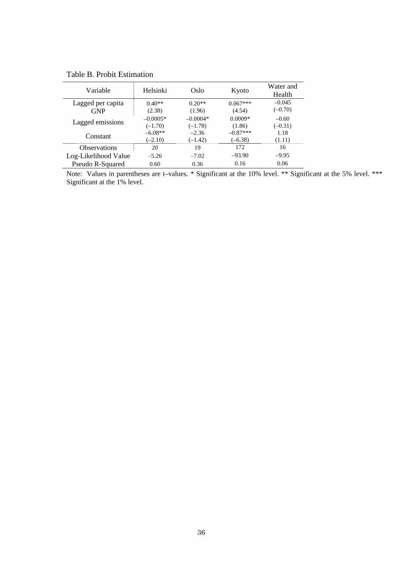
For the Helsinki Protocol, Oslo Protocol, and Kyoto Protocol, we obtained

statistically significant results that are almost in line with the expected sign. The only

exception is the sign of lagged emissions for the Kyoto Protocol. On the other hand, we

are not able to obtain a statistically significant result for the Protocol on Water and

Health. Predicted probabilities are calculated and are then imputed to the original

Helsinki, Oslo, and Kyoto Protocol variables.

36

Table B. Probit Estimation

Note: Values in parentheses are t–values. * Significant at the 10% level. ** Significant at the 5% level. *** Significant at the 1% level.

Variable Helsinki Oslo Kyoto Water and Health

Lagged per capita GNP

0.40** (2.38)

0.20** (1.96)

0.067*** (4.54)

–0.045 (–0.70)

Lagged emissions –0.0005* (–1.70)

–0.0004* (–1.78)

0.0009* (1.86)

–0.60 (–0.31)

Constant –6.08** (–2.10)

–2.36 (–1.42)

–0.87*** (–6.38)

1.18 (1.11)

Observations 20 19 172 16 Log-Likelihood Value –5.26 –7.02 –93.90 –9.95

Pseudo R-Squared 0.60 0.36 0.16 0.06

37

Appendix C. Data and the List of the Countries Used for This Study

List of the countries used for this study is provided in Table C.

Table C. Lists of the Country in This Study North America Uruguay Belgium Gambiaa

Canada Venezuela Britain Ghana USA Asia Cyprus Kenya Latin America Bangladesh Denmark Malawi

Argentine China Finland Malib

Barbados Hong Kong France Mauritaniab

Bolivia India Greece Mauritius

Brazil Indonesia Hungary Mozambique Chile Japan Iceland Niger

Colombia Korea Ireland Rwanda

Costa Rica Malaysia Italy Senegal Dominica Nepal Netherlands Sierra Leoneb

Ecuador Pakistan Portugal South Africa El Salvador Philippines Romania Togo Guatemala Singapore Spain Tunisia Guiana Sri Lanka Sweden Uganda

Haitib Thailand Switzerland Zambia Honduras Middle East Africa Zimbabwe Jamaica Iran Beninb Oceania Mexico Israel Burundib Australia Nicaragua Jordan Cameroon Fiji

Panama Syria Central Africa New Zealand Paraguayb Turkeya Congo Peru Europe Egypt Trinidad and Tobago Austria Ethiopia Note a Not included in SO2 and CO2 specification. b Not included in BOD specification

Simple scatter plots are portrayed in Figure C, where there are not rough

correlation between emissions and trade.

38

SO2 emissions per capita against Trade openness CO2 emissions per capita against Trade openness BOD emissions per capita against Trade openness

SO2 emissions per capita against GDP per capita CO2 emissions per capita against GDP per capita BOD emissions per capita against GDP per capita

SO2 emissions per capita against Capital–labor ratio CO2 emissions per capita against Capital–labor ratio BOD emissions per capita against Capital–labor ratio

GDP per capita against Trade openness Capital–labor ratio against Trade openness GDP per capita against Capital–labor ratio

Fig. C. Simple scatter plots of data Note: Vertical axis and horizontal axis are expressed as follows. In the case that the figure title is “A

against B”, vertical axis and horizontal axis corresponds to A and B, respectively. SO2 emissions per

capita, CO2 emissions per capita and BOD emissions per capita are measured in kg, tons and kg,

respectively. Trade openness, real GDP per capita and Capital–labor ratio are measured in %, $ and

capital per worker, respectively.

0

100

0 100 200 300 400

0

20000

40000

0 20000 60000 1000000

40000

80000

0 100 200 300 400 0

20000

40000

0 100 200 300 400

0

10

0 20000 60000 1000000

10

20

20000 60000 1000000

100

0 20000 60000 100000

0

10

0 10000 20000 30000 0

10

20

0 10000 20000 300000

100

0 10000 20000 30000

0

10

0 100 200 300 400 0

10

20

0 100 200 300 400

39

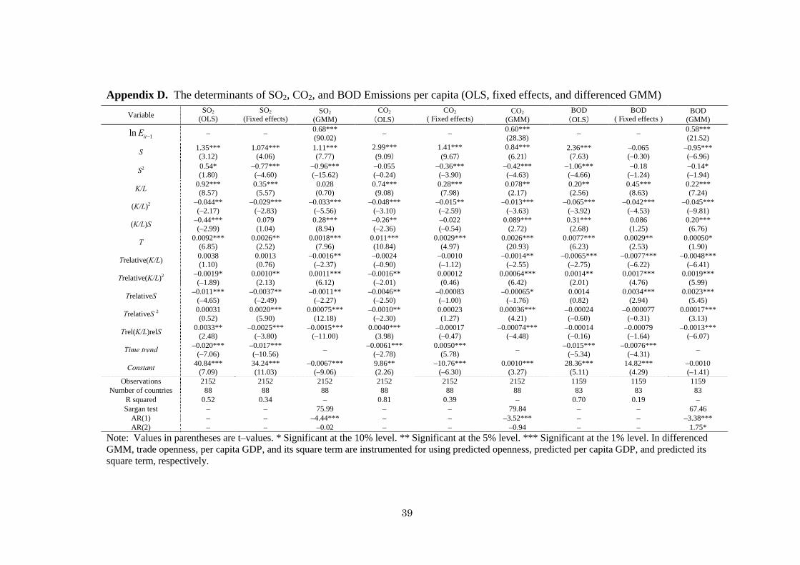
Appendix D. The determinants of SO2, CO2, and BOD Emissions per capita (OLS, fixed effects, and differenced GMM)

Note: Values in parentheses are t–values. * Significant at the 10% level. ** Significant at the 5% level. *** Significant at the 1% level. In differenced GMM, trade openness, per capita GDP, and its square term are instrumented for using predicted openness, predicted per capita GDP, and predicted its square term, respectively.

Variable SO2 (OLS)

SO2 (Fixed effects)

SO2 (GMM)

CO2 （OLS）

CO2 ( Fixed effects)

CO2 (GMM)

BOD （OLS）

BOD ( Fixed effects )

BOD (GMM)

1ln itE − – – 0.68***

(90.02) – – 0.60*** (28.38) – – 0.58***

(21.52)

S 1.35*** (3.12)

1.074*** (4.06)

1.11*** (7.77)

2.99*** (9.09)

1.41*** (9.67)

0.84*** (6.21)

2.36*** (7.63)

–0.065 (–0.30)

–0.95*** (–6.96)

S2 0.54* (1.80)

–0.77*** (–4.60)

–0.96*** (–15.62)

–0.055 (–0.24)

–0.36*** (–3.90)

–0.42*** (–4.63)

–1.06*** (–4.66)

–0.18 (–1.24)

–0.14* (–1.94)

K/L 0.92*** (8.57)

0.35*** (5.57)

0.028 (0.70)

0.74*** (9.08)

0.28*** (7.98)

0.078** (2.17)

0.20** (2.56)

0.45*** (8.63)

0.22*** (7.24)

(K/L)2 –0.044** (–2.17)

–0.029*** (–2.83)

–0.033*** (–5.56)

–0.048*** (–3.10)

–0.015** (–2.59)

–0.013*** (–3.63)

–0.065*** (–3.92)

–0.042*** (–4.53)

–0.045*** (–9.81)

(K/L)S –0.44*** (–2.99)

0.079 (1.04)

0.28*** (8.94)

–0.26** (–2.36)

–0.022 (–0.54)

0.089*** (2.72)

0.31*** (2.68)

0.086 (1.25)

0.20*** (6.76)

T 0.0092*** (6.85)

0.0026** (2.52)

0.0018*** (7.96)

0.011*** (10.84)

0.0029*** (4.97)

0.0026*** (20.93)

0.0077*** (6.23)

0.0029** (2.53)

0.00050* (1.90)

Trelative(K/L) 0.0038 (1.10)

0.0013 (0.76)

–0.0016** (–2.37)

–0.0024 (–0.90)

–0.0010 (–1.12)

–0.0014** (–2.55)

–0.0065*** (–2.75)

–0.0077*** (–6.22)

–0.0048*** (–6.41)

Trelative(K/L)2 –0.0019* (–1.89)

0.0010** (2.13)

0.0011*** (6.12)

–0.0016** (–2.01)

0.00012 (0.46)

0.00064*** (6.42)

0.0014** (2.01)

0.0017*** (4.76)

0.0019*** (5.99)

TrelativeS –0.011*** (–4.65)

–0.0037** (–2.49)

–0.0011** (–2.27)

–0.0046** (–2.50)

–0.00083 (–1.00)

–0.00065* (–1.76)

0.0014 (0.82)

0.0034*** (2.94)

0.0023*** (5.45)

TrelativeS 2 0.00031 (0.52)

0.0020*** (5.90)

0.00075*** (12.18)

–0.0010** (–2.30)

0.00023 (1.27)

0.00036*** (4.21)

–0.00024 (–0.60)

–0.000077 (–0.31)

0.00017*** (3.13)

Trel(K/L)relS 0.0033** (2.48)

–0.0025*** (–3.80)

–0.0015*** (–11.00)

0.0040*** (3.98)

–0.00017 (–0.47)

–0.00074*** (–4.48)

–0.00014 (–0.16)

–0.00079 (–1.64)

–0.0013*** (–6.07)

Time trend –0.020*** (–7.06)

–0.017*** (–10.56) – –0.0061***

(–2.78) 0.0050***

(5.78) – –0.015*** (–5.34)

–0.0076*** (–4.31) –

Constant 40.84*** (7.09)

34.24*** (11.03)

–0.0067*** (–9.06)

9.86** (2.26)

–10.76*** (–6.30)

0.0010*** (3.27)

28.36*** (5.11)

14.82*** (4.29)

–0.0010 (–1.41)

Observations 2152 2152 2152 2152 2152 2152 1159 1159 1159 Number of countries 88 88 88 88 88 88 83 83 83

R squared 0.52 0.34 – 0.81 0.39 – 0.70 0.19 – Sargan test – – 75.99 – – 79.84 – – 67.46

AR(1) – – –4.44*** – – –3.52*** – – –3.38*** AR(2) – – –0.02 – – –0.94 – – 1.75*

40

Appendix E. The results for NOx

We obtain NOx emissions data from The Emission Database for Global

Atmospheric Research (EDGAR) for 1990, 1995, and 2000, meaning that the data is

available for only three years. The decision to ratify the Sofia Protocol29 occurred in

1988 and the first year of data is from 1990, so we did not use a probit model. Instead,

we use a simple dummy variable that takes a value of 1 if the country has already

ratified the 1988 Sofia protocol and 0 otherwise. Table F-1 presents the estimated

parameters of equation (1) using differenced GMM, while Table F-2 presents the

trade-induced elasticities evaluated at the sample means. As is shown in Table F-2, the

elasticities of the trade-induced scale-technique effect, STσ , are statistically significant

with a positive sign in all cases. This result indicates that the scale effect dominates the

technique effect. The elasticities of the trade-induced composition effects, Cσ , and of

the overall effect, Tσ , are insignificant.

29 This required the countries in the United Nations Economic Commission for Europe that signed the Protocol to stabilize emissions of NOx against 1987 levels by 1994, and some countries committed themselves to 30% reductions by 1998 (against levels of any year between 1980 and 1986).

41

Table E-1. The determinants of NOx Emissions per capita (Differenced GMM)

Note: Values in parentheses are t–values. * Significant at the 10% level. ** Significant at the 5% level. ***Significant at the 1% level. Trade openness, per capita GDP, and its square term are instrumented for usingpredicted openness, predicted per capita GDP, and predicted its square term, respectively.

Variable NOx （Protocol） NOx

1ln itE − –0.80 (–1.64)

–0.90* (–1.88)

S 2.73* (1.73)

2.79* (1.71)

S2 3.05* (1.72)

3.47* (1.97)

K/L 0.18 (0.34)

0.24 (0.46)

(K/L)2 0.19** (2.12)

0.21** (2.45)

(K/L)S –1.73** (–2.04)

–1.95** (–2.36)

T 0.0073* (1.67)

0.0075* (1.76)

Trelative(K/L) 0.018 (1.37)

0.015 (1.18)

Trelative(K/L)2 –0.0071 (–0.73)

–0.0096 (–1.06)

TrelativeS –0.023** (–2.47)

–0.022** (–2.34)

TrelativeS 2 –0.0019 (–0.47)

–0.0033 (–0.88)

Trel(K/L)relS 0.011 (0.85)

0.016 (1.29)

Sofia Protocol 0.18 (1.24) –

Constant 0.29*** (5.27)

0.29*** (5.19)

Observations 69 69 Number of countries 69 69

Sargan test 5.40 5.69 AR(1) – – AR(2) – –

42

Table E-2. Trade Elasticity (Differenced GMM) Short Term Long Term Elasticity

NOx NOx

STσ 0.482* 1.951*

OCσ –0.404** –1.636**

ITCσ –0.002* –0.007* Cσ

DTCσ

–0.819

–0.413 –2.172

–0.217 OECD

Tσ –0.337 0.092

STσ 0.049* 0.200*

OCσ –0.022** –0.090**

ITCσ –0.000* –0.001* Cσ

DTCσ

–0.346

–0.324 –0.098

–0.170 Non-OECD

Tσ –0.297 –0.061

STσ 0.130* 0.525*

OCσ –0.085** –0.343**

ITCσ –0.001** –0.002* Cσ

DTCσ

0.695

–0.609 –0.505

–0.320 All data

Tσ –0.565 –0.141

Note: * Significant at the 10% level. ** Significant at the 5% level. *** Significant at the 1% level.

43

Appendix F. Why the Results are Different from Previous Studies?

This paper is an improvement on papers by Antweiler et al. (2001) and Cole and

Elliott (2003). By applying instrumental variables and using data from more years and

countries, we find different results. Therefore, it is critical to understand where the

differences come from.

First, we try to replicate the results of Antweiler et al. (2001) and Cole and Elliot

(2003). We apply fixed effects estimation methods to the closest possible approximation

to previous studies’ data sets in terms of emissions data and country and year

coverage.30 We calculate the scale-technique effect31 and DTCσ and compare them

with previous studies’ trade-induced effects. We are able to obtain similar elasticities to

those found in previous studies, as shown in Table F-1,32 although some elasticities are

not statistically significant.

Second, to clarify how important our instruments are, we also apply OLS

estimation and differenced GMM estimation to the same data. We present STσ and

DTCσ as calculated using OLS estimation, fixed effects estimation, and differenced

30 Although we tried to obtain the same data as previous studies, we were not able to obtain exactly

the same data. To replicate Cole and Elliot (2003), we collected emissions data from the same data

source as theirs. However, we did not obtain a complete set of years and countries. More specifically,

we were able to collect data from 24 out of 26 countries for SO2, 26 out of 32 countries for CO2, and

25 out of 32 countries for BOD, and we were not able to obtain BOD data for 1975-1979. On the

other hand, to replicate Antweiler et al. (2001), we used our emissions data for the countries and

years in their paper, and we apply the same specification as ours because of data limitations. We are

able to collect emissions data for SO2 for 36 out of the 43 countries in Antweiler et al. (2001). 31 Note that we calculate the scale-technique effect, not the trade-induced scale-technique effect. 32 Exceptions are DTCσ for SO2 from Antweiler et al. (2001) and DTCσ for BOD from Cole and

Elliot (2003). These seem to be different because we were not able to obtain a complete data set to

match those used in previous studies.

44

GMM estimation in sections (a), (b), and (c) of Table F-2 respectively. There may be

other factors such as autocorrelation and heteroskedasticity that could bias the results of

the OLS estimation. We obtained different results from the OLS and GMM estimates,

which might imply that we need to take these factors into consideration. In addition, we

obtain different elasticities using fixed effects and GMM, which also might imply that

including instrumental variables has an impact on the results.

Third, to consider the effect of updating data, we perform a fixed effects

estimation using the data in this study. Section (d) of Table F-2 shows the elasticities

found using fixed effects as well as the elasticities found using OLS and differenced

GMM estimation. These estimates come from our original data set33. We find that the

change in data used has a small effect on the elasticities compared to the change in

estimation methods. Therefore, we conclude that the differences between the results of

Antweiler et al. (2001), Cole and Elliot (2003), and our study seem to stem mainly from

differences in estimation methods rather than differences in data used. In other words, it

is important to take endogeneity into consideration.

Table F-1. Replication of previous studies (Fixed effects)

Note: * Significant at the 10% level. ** Significant at the 5% level. *** Significant at the 1% level. Elasticities are evaluated at sample means.

Effect SO2 CO2 BOD Reproduced directly from Cole and Elliott (2003) –1.7** 0.46*** –0.06***

Our Replication of Cole and Elliot (2003) –0.491 0.094*** –0.031 Reproduced directly from Antweiler et al. (2001) –0.332**

Scale-technique effect (cf. trade-induced scale-

technique effects) Our Replication of Antweiler et al. (2001) –0.887*** Reproduced directly from Cole and Elliott (2003) 0.3*** 0.049* –0.05***

Our Replication of Cole and Elliot (2003) 0.631* 0.151** 0.112* Reproduced directly from Antweiler et al. (2001) –0.864*** DTCσ

Our Replication of Antweiler et al. (2001) 0.108*

33 We present parameter estimates of OLS, fixed effects, and differenced GMM using the data in

this study in Appendix D.

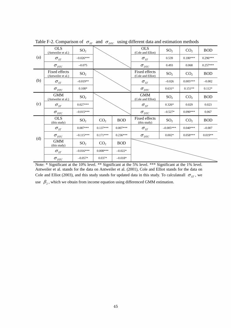
45

Table F-2. Comparison of STσ and DTCσ using different data and estimation methods OLS

(Antweiler et al.) SO2 OLS

(Cole and Elliot) SO2 CO2 BOD

STσ –0.026*** STσ 0.539 0.180*** 0.296*** (a)

DTCσ –0.075

DTCσ 0.493 0.068 0.257***

Fixed effects (Antweiler et al.)

SO2 Fixed effects (Cole and Elliot)

SO2 CO2 BOD

STσ –0.019** STσ –0.026 0.005*** –0.002 (b)

DTCσ 0.108*

DTCσ 0.631* 0.151** 0.112*

GMM (Antweiler et al.)

SO2 GMM (Cole and Elliot)

SO2 CO2 BOD

STσ 0.027*** STσ 0.326* 0.029 0.023 (c)

DTCσ –0.015***

DTCσ –0.527* 0.090*** 0.067

OLS (this study)

SO2 CO2 BOD Fixed effects (this study)

SO2 CO2 BOD

STσ 0.087*** 0.137*** 0.007*** STσ –0.005*** 0.040*** –0.007

DTCσ –0.115*** 0.171*** 0.236*** DTCσ 0.002* 0.058*** 0.019**

GMM (this study) SO2 CO2 BOD

STσ –0.016*** 0.008*** –0.022*

(d)

DTCσ –0.057* 0.037* –0.018*

Note: * Significant at the 10% level. ** Significant at the 5% level. *** Significant at the 1% level. Antweiler et al. stands for the data on Antweiler et al. (2001), Cole and Elliot stands for the data on Cole and Elliot (2003), and this study stands for updated data in this study. To calculateall STσ , we

use 2β , which we obtain from income equation using differenced GMM estimation.