Does emissions trading lead to air pollution hot spots ...

Does emissions trading lead to air pollution hotspots? Evidence from an urban ozone controlprogramme

Richard F. Kosobud*, Houston H. Stokesand Carol D. TallaricoDepartment of Economics, University of Illinois at Chicago,Chicago, Illinois, USAFax: 312 996 3344 E-mail: [email protected]*Corresponding author

Abstract: This study is an empirical investigation into the contentious issueof possible sub-area hot spots caused by emissions trading in a pioneeringapplication of a cap-and-trade market approach to reducing aggregatestationary-source volatile organic compound emissions in the Chicago severeozone non-attainment region. When sub-areas are defined as populated zipcodes, 89 out of 95 affected codes revealed a decrease and six an increase inemissions over pre-trading levels. If these six sub-areas are increased slightly insize by adding adjacent zip codes, emissions will be reduced in all sub-areas.Those sub-areas with the largest initial emissions revealed the most significantreductions after trading. The study also finds that trading has significantly reducedboth aggregate market-wide levels and the variation in sub-area emissions frompre-trading patterns. Spatially constraining the present region-wide market topre-empt possible future hot spots could reduce savings in pollution controlcosts by over 40%.

Keywords: cap-and-trade market; emissions trading; pollution control costsavings; spatial pollution hot spots.

Reference to this paper should be made as follows: Kosobud, R.F., Stokes, H.H.and Tallarico, C.D. (2004) ‘Does emissions trading lead to air pollution hotspots? Evidence from an urban ozone control programme’, Int. J. EnvironmentalTechnology and Management, Vol. 4, Nos. 1/2, pp.137–156.

Biographical notes: Richard Kosobud is Professor of economics with an interestin market-based approaches to environmental policy. His most recent booksinclude Emissions Trading: Environmental Policy’s New Approach, (John Wiley& Sons, 2000), and Market-Based Approaches to Environmental Policy, (VanNostrand Reinhold, 1997). He has published numerous articles in leadingjournals. His research has been supported by the Illinois EnvironmentalProtection Agency, the National Science Foundation and the John T. andCatherine D. MacArthur Foundation, among other sponsors.

Houston Stokes is Professor of economics with interests in energy economics,applied econometrics, statistical software development, time series analysis,and international trade. He is the developer of the B34S® Software system andhas over 75 papers and four books in print. The books include Unemploymentand Adjustment in the Labor Market, with Hugh Neuburger and Donald Jones,(University of Chicago Press, 1975), Specifying and Diagnostically TestingEconometric Models (Quorum Books 1991, 1997) and New Methods in FinancialModeling, with Hugh Neuburger, (Quorum Books, 1998).

Int. J. Environmental Technology and Management, Vol. 4, Nos. 1/2, 2004 137

Copyright © 2004 Inderscience Enterprises Ltd.

11_Kosobud 5/5/04 2:21 pm 37

Carol Tallarico is a Visiting Lecturer of economics and currently completing herPhD in economics. She obtained her BA in international studies in 1998 and herMA in economics in 1999 from DePaul University. Her primary interests areinternational economics, growth economics, time series and econometrics, andenvironmental economics.

1 Introduction

The spatial relationship of harmful environmental externalities to adjoining populationshas received increased attention recently in the US with a focus on the location ofincinerators, Toxic Release Inventory (TRI) emitters, landfills, and National Priority ListSuperfund areas [1]. This study addresses a new and quite different issue in the matter ofspatial pollution impacts: does market-based incentive regulation, although reducingmarket-wide pollution, lead to sub-area increases (hot spots) in pollution over baselineaffecting nearby resident populations? Specifically, we compare the before and afterspatial distribution of pollution that results from the application of a new mandatorycap-and-trade market programme to reduce stationary-source emissions of volatile organiccompounds (VOC) in the Chicago severe ozone non-attainment region. This marketincentive programme replaced traditional regulation that determined the before-tradingsub-area distribution.

The Chicago region contains almost 200 stationary-source VOC emitters widelyscattered about a large urban region with varied socio-economic groups residing closeby. Our objective is to analyse the after-trading pattern to see what changes werebrought about by this novel programme in the existing distribution of emissions. In sharpcontrast, the great majority of prior studies investigating spatial disamenities, or issuesof environmental justice or equity, have been concerned with the siting or location ofpollution sources and the definition of affected populations in terms of class and race.A review of the issues and literature on these concerns is provided in this journal byHaynes et al. [1]. Our focus being different, we can move quickly to an analysis ofsub-area emission changes brought about by trading.

Compared with traditional regulation, the autonomy and anonymity of transactionsin the cap-and-trade market make increases in emissions in sub-areas more difficultto predict and can thus raise some concerns about spatial impacts. Moreover, marketincentive programmes are of recent origin with few studies of spatial pollution patternsavailable. It would appear that traditional regulation has a spatial or sub-area advantage inthat pollution is reduced in all affected sub-areas by the same proportion becausetraditional regulation typically sets performance standards or fixed rates of emissionsper unit time for certain processes (or pipes), often requiring the same pollution controltechnologies for all emitters [2]. However, appreciable variations in the hours of productionof existing firms and movements of new firms into a sub-area can increase emissions overhistorical or baseline values. Thus, increases in sub-area emissions over the baseline canoccur under both traditional and market-incentive regulation. A careful empirical beforeand after analysis is required in both cases.

138 R.F. Kosobud, H.H. Stokes and C.D. Tallarico

11_Kosobud 5/5/04 2:21 pm Page 138

To explain our analysis and findings in detail, this study is divided into the followingsections. We first describe how a cap-and-trade market may rouse concerns aboutdifferential spatial impacts caused by emissions trading. We next discuss the choice ofa sub-area for the before and after analysis of trading. We then explain our before andafter methods of detecting actual hot spots including a detailed account of our databases.Our results are displayed in maps and histograms relating emissions to sub-areas andpopulation characteristics. We then raise the question of the possible policy response tohot spot concerns, and examine subdividing the market as one response. We introduce aspecially designed cost-minimisation model based on individual emitter marginal controlfunctions to estimate the loss in pollution control cost savings that would result from suchsubdivisions. We conclude with a discussion of directions for further research.

2 The invisible hand of the market and concern about hot spots

The success in reducing market-wide aggregate pollution in the highly regarded US sulphurdioxide or acid rain emissions trading programme [3] has not alleviated all concerns thatemissions trading in the cap-and trade market design can lead to sub-area or inter-temporalincreases in air pollution over baseline or historic emissions, as expressed by Drury et al.[4]. Only detailed spatial studies and an understanding of emissions trading can dealadequately with these concerns.

Under the mandated cap-and-trade market incentive approach of the Chicagoprogramme, the Illinois Environmental Protection Agency (Illinois EPA) decentralisedpollution control decisions to the firm but retained the power to set the aggregate cap (inthis case at a 12% reduction from historic or baseline levels) and to monitor and enforcemarket rules and VOC emissions reporting. Firms were allotted free of charge tradablepermits as a fraction (0.88 with some adjustment for special circumstances) of theirhistoric or baseline emissions. They could sell permits anywhere in the region, buy fromanyone in the region, and bank permits for one year. The unified spatial market wasadopted in the interest of maximising potential control-cost savings from trading. Thebasic rule of the market is that an emitter must turn over to the agency a tradable permitfor each 200 pounds of VOC emissions [5].

Under the region’s cap-and-trade policy, continuing traditional regulation sets apre-trading ceiling on an individual firm’s emissions that would appear to prohibit anysub-area increases over that level, but it is possible for these increases to occur if existingfirms expand production or if new firms move into the sub-area. Neither the expanded northe new firm would be allocated additional tradable credits but they could enter the marketto buy what was required. There are no restrictions on the market that would preventsuch increases from occurring. On the contrary, it is expected that firms that can reduceemissions cheaply will do so and sell permits to firms for whom reducing emissions ismore expensive than purchasing permits, thus achieving cost savings in comparison withtraditional regulation [6].

In a competitive cap-and-trade market in which firms have varying marginal pollutioncontrol costs, it is expected that firms will reduce emissions by various percentages,implying that it should be advantageous for some firms to increase emissions over theirallotment [7]. As the micro-decisions about reducing emissions or trading are now inthe hands of the emitters, independent of the regulating agency, the spatial pattern of

Does emissions trading lead to air pollution hot spots? 139

11_Kosobud 5/5/04 2:21 pm Page 139

emissions becomes evident only at the end of the ozone period, from May to September,when emitters must report their emissions and turn over to the Illinois EPA the correctnumber of tradable credits.

3 Delineating the appropriate sub-area and its relation to potential hot spots

How to specify an appropriate sub-area to investigate increased emissions or hot spots andthe associated harm function are among the most difficult topics in the analysis of spatialenvironmental analysis. This is clearly true in the case of VOC emissions and ozoneconcentrations [8]. It is to be noted that these are fund pollutants that dissipate in theatmosphere over time. VOC emissions, in addition to being a precursor of ozone, can beharmful to health in their own right. They arise from a wide variety of processes in theregion ranging from candy making, to plating, to painting cars, and on to the refiningof crude oil. The hydrocarbon stream may be scrubbed, burned, absorbed in carbon, orreduced in production inputs such as less emitting paints, glues, and the like [9]. Whatremains will diffuse in space from vents, pipes, chimneys, or other openings. The spatialspread of hydrocarbons is difficult to model since the range of emissions and formationof concentrations depend on meteorology and chemical reactions, among other variables.

3.1 The sub-area harm function

The effect of emission exposure on the population depends on the number of sensitivepeople, inside and outside activities, and the concentration of hydrocarbons at the pointof contact, and other variables. While there has been some research on the general harmsof low-level ozone reported in Tolley [10], there has been less research on the harms ofvolatile organic compounds including those that are hazardous air pollutants, and muchless research on local effects [11]. The US Toxic Substances Control Act requires testingrules for each chemical but only a few such rules have been promulgated by the US EPA.Monitoring of ambient air quality and emissions from individual or sub-area sourcesis proving to be more complex and costly than once believed. Setting zero risk orzero emissions for a source, or sub-area, is either prohibitively expensive, or simplyimpossible [12].

Low-level ozone concentrations formed as a result of combinations of precursors suchas VOCs, nitrogen oxides, and weather conditions, follow complex spatial paths aroundthe area. The several dozen scattered monitoring stations in the area indicate that theozone plume is generally moved across and out of the region by the prevailing summersouthwesterly winds frequently carrying the concentrations during hot summer monthsdeep into the neighbouring State of Wisconsin and across Lake Michigan to localities inthe State of Michigan such as Muskegon. Specific sub-area concentrations are difficult tomeasure and predict and yield little guidance on an appropriate sub-area for measuringharms [13,14].

Lacking detailed knowledge of how to measure sub-area harms accurately, we focuson VOC emissions and adopt a proximity ‘surrogate’ harm function that relates harmsof this pollutant to the immediate area surrounding the sources of emissions. For ourpurposes, after balancing a number of factors, a hot spot is specified as a sub-area with apopulation where VOC emissions have increased due to trading over the pre-trading orbaseline level.


11_Kosobud 5/5/04 2:21 pm Page 140

3.2 The appropriate sub-area

The Chicago non-attainment region covers all of six counties and parts of two others.There are 118 townships averaging 32 square miles in area, 298 zip codes varying in areabut averaging 13 square miles, and hundreds of census tracts varying widely in area.The counties appear too large in area to reveal hot spots in the detail we require, asTable 1 demonstrates. All counties exhibit a decrease in emissions ranging from 25.4 to55.9%. The townships, a local government area, have been analysed by the Illinois EPAbut leave scope for more detail. The census tract appears to provide too much detail forclear mapping analysis and portrayal.


Table 1 Population, emitters, before and after-trading emissions by county

County Population Number Baseline After-trading Percentname (1999 number) of emitters emissions emissions change in

of people) (200 lbs) (200 lbs) emissions

Cook 5,192,105 116 72,130 39,127 �45.90%

DuPage 890,164 11 4379 1932 �55.90%

Grundy 37,213 2 4944 3049 �38.40%

Kane 401,360 13 4328 2970 �31.50%

Kendall 53,914 1 614 459 �25.40%

Lake 616,422 10 4727 3210 �32.20%

McHenry 246,533 8 1887 995 �47.50%

Will 474,617 19 12,471 7303 �41.50%

Total 7,912,328 180 105,479 59,045 �44.00%

Note: Population data are 1999 estimates by CACI International Inc. All other data from Illinois EPA AnnualNote: Performance Review Report of 2000 and 2001 [5]. Only a few townships included in Grundy and

Kendall counties are included in the severe ozone non-attainment region, but population estimates arefor the entire county.

The zip code, a US Postal Service area for mail delivery, appears to be the best compromisein terms of area and neighbourhood delineation. The zip code has been chosen as thesub-area for other studies of hot spots as in the California Comparative Risk Project [15].It also is a spatial unit for which population and socio-economic data are available. Thereare 298 zip codes in the non-attainment area 95 of which contain one or more VOCemitters in their boundaries. These 95 are the potential candidates to be tested by our hotspot definition.

11_Kosobud 5/5/04 2:21 pm Page 141


3.3 The databases

The Illinois EPA has provided us with emitter addresses, tradable credit allotments,tradable credit retirements (actual emissions during the year 2000), and tradable creditpurchases and sales, from which banks may be calculated. Given the allotments andpolicy cap, we were able to estimate the baseline emissions for each enterprise. Theagency also made available breakdowns for those emitters for whom some or all of theirVOC emissions were hazardous air pollutants such as benzene. However, specific data onHAP emissions are not yet available. Much of these data were presented in spreadsheetformat, and can be provided to researchers. Valuable supplementary data are presented inthe first annual evaluation reports of the Illinois EPA [5].

The agency has made a number of quality control checks to validate reported emissionsdata. This is an important function of the government, since systematic errors in emissionsdata would affect the creditability of the tradable emission permit and the reliability of ourhot spot analysis. Over 50% of the market participants were visited during 2001 to checkrecord keeping and VOC control equipment and processes. Violations were detected inseven cases with corrections made to the data. Further checks were made on 59 submittedreports with four minor record keeping errors detected and corrected [5].

4 Detection and analysis of actual hot spots in the year 2000 due toemissions trading

4.1 Mapping the before-trading zip code distributions of population andbaseline emissions

The city of Chicago has a population of about three million out of almost eight million inall affected counties. The city centre is located along the lake about halfway up CookCounty as revealed in the map of Figure 1. The areas of greatest population density, whichare also areas of residence of low income and minority populations, are located on thenear west and south sides of the city centre. The city north side area is also densely settled,but the residence of more middle and upper income households. Other concentrationsof population, mainly middle income, may be seen in northwest Cook County and on thewest in DuPage County.

Baseline emissions are before-trading emissions and the zip code distribution revealedin the Figure 2 map is the result of years of traditional regulation, frequently termedcommand-and-control. Baseline emissions also reveal the location of the almost 200major emitters covered by the cap-and trade market. A concentration of emissions isrevealed on the near south and southwest sides of the city, areas of residence of lowincome and minority populations, and a concentration on the northwest side of CookCounty in a more middle income area.

11_Kosobud 5/5/04 2:21 pm Page 142


Figure 1 1999 estimated population by zip code. Total population is 7,912,328 people for theeight county area. Total population in zip codes with emitters is 3,215,295

11_Kosobud 5/5/04 2:21 pm Page 143


Figure 2 Year 2000 baseline emissions in 200-pound units of VOC by zip code

11_Kosobud 5/5/04 2:21 pm Page 144


Another interesting aspect of these zip code distributions is that the correlation coefficientbetween population and baseline emissions is not significantly different from zero. It isapparent that some zip codes have a large population and large volumes of emissions, butthis link is offset by the distribution of emitters in outlying areas where land is cheaper,transportation more rapid, and population densities less. Some large emitters such as the3M Corp., BP Amoco refinery, Corn Products Co. and the Abbott Labs Co. are found inthese outlying areas surrounded by small populations.

4.2 Mapping the after-trading zip code distribution of emissions

The striking impression of the map of Figure 3 is that emissions have been reducedby trading in almost all zip codes, and the variation and range of emissions have beensignificantly reduced. Of special interest is the reduction in emissions in the denselysettled city centre areas with their concentrations of low-income and minority populations.

On another spatial dimension, a significant finding is the changes in the meansand variances of the before and after-trading zip code distributions, and the reductions inthose codes with the greatest volumes of emissions. These changes are brought out in thehistograms of Figure 4a and b.

Figure 4a provides a histogram view of the range of pre-trading emissions by zipcode by arraying codes from highest to lowest baseline emissions along the abscissa, andplotting baseline emissions along the ordinate. It may be seen from the diagram that thetop 20 zip codes account for well over 50% of all emissions. These codes are of specialinterest to the extent that local emissions inflict harms on the local population.

The reduction in emissions in almost all zip codes after trading is brought out in thehistogram of Figure 4b where zip codes are once again arrayed from high to low in termsof baseline emissions along the abscissa, but the ordinate now portrays after-tradingemissions. The mean emission value for zip codes with emitters prior to trading was 1132of VOC 200 pound units with a standard deviation of 2176; the mean declines to 643 unitsafter trading with a standard deviation of 1396.

Trading has brought about a significant reduction in the top 20 codes with highestbefore-trading pollution volumes. If zip codes are arrayed on the abscissa from highestto lowest after-trading emissions (not shown) with after trading-emission volumes onthe ordinate, the top 20 codes revealed a marked reduction in the mean and standarddeviation. The mean is reduced from 3611 to 2033, measured in 200-pound units, and thestandard deviation is reduced from 3848 to 2617. This is in sharp contrast with the muchsmaller changes revealed among the lowest 20 zip codes in volume where the mean isreduced from 166 to 105 and the standard deviation from 43.3 to 42.9. We interpret thesechanges to be indications that local harm has been reduced in those sub-areas where it wasmost significant.

11_Kosobud 5/5/04 2:21 pm Page 145


Figure 3 Year 2000 after-trading emissions in 200-pound units of VOC by zip code

11_Kosobud 5/5/04 2:21 pm Page 146


Figure 4 (A) Baseline or pre-trading emissions by zip code in 200-pound units of VOC.(B) After-trading emissions by zip code in 200-pound units of VOC

(a)

(b)

11_Kosobud 5/5/04 2:21 pm Page 147


4.3 Mapping the sub-area zip code distribution of reductions or increases inemissions after trading

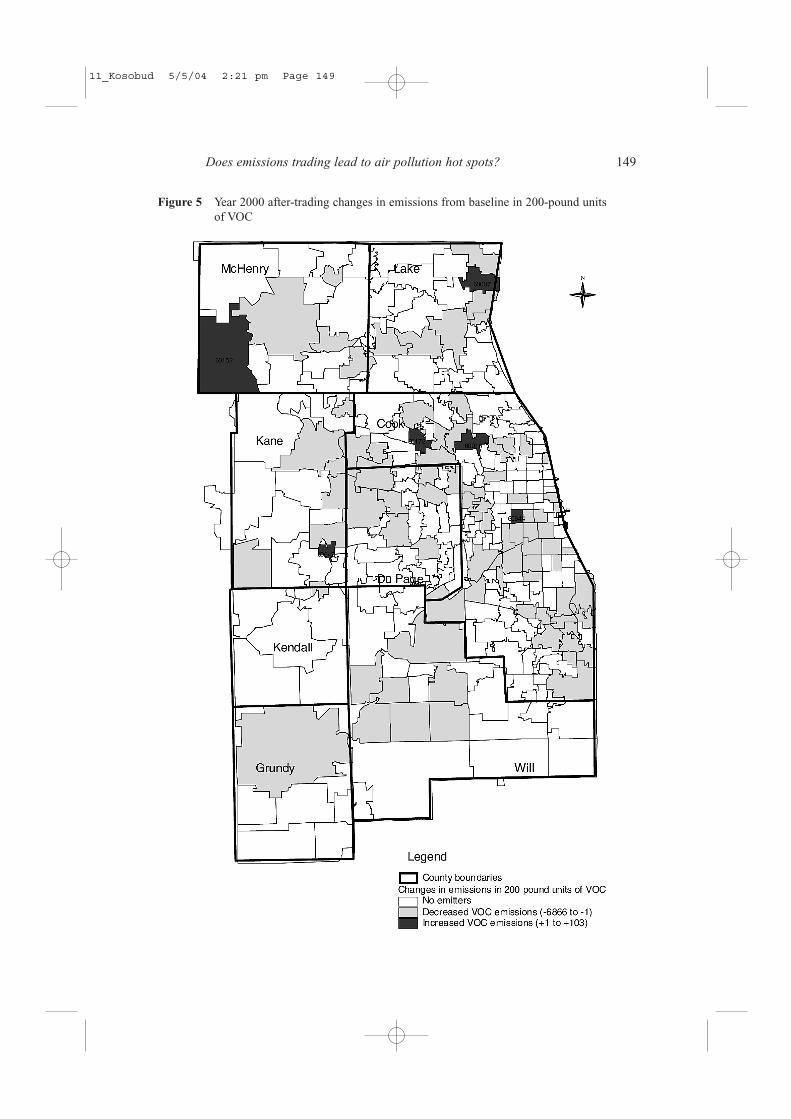
The Figure 5 map brings together the maps of Figures 2 and 3 and reveals more clearlythe decreases or increases in 200-pound units of emissions by zip code due to trading.Zip codes with no emitters and no emissions are left blank. The six zip codes revealingincreases are isolated and scattered about the region. The significant reduction in allbut one of the zip codes (60644) with resident low-income and minority populationsis noteworthy.

To further evaluate those six zip codes, we have prepared in Table 2 a list of thesecodes together with their population, their baseline and their after-trading emissions. Thepopulation of the six codes is about 5% of the region’s population living in zip codeswith emission sources. These six codes emitted slightly less than 5% of the region’s VOCemissions in the year 2000. Among the six were two codes where we could estimatean increase in hazardous air pollutant discharges by assuming a fixed proportion of thesedischarges to other VOC emissions. These two codes had about 3% of the region’spopulation in affected areas and less than 1% of the stationary-source VOC emissions.Adding new processes and extending hours, both of which required emitters to purchaseadditional tradable credits, were mainly responsible for the emissions increase over baselinein the six codes.

The question of the sensitivity of our spatial measure to incremental changes in thearea arises in the case of these six codes. One plausible change would be to enlarge eachof the codes by adding the abutting zip codes that contained emissions. As may be seenin Figure 5, that meant adding one abutting code to two of the original six, adding twocodes to two of the six, and adding three codes to the remaining two of the six. When thisis done, we obtain the important result that in all of the newly defined sub-areas, theincreases in emissions due to trading were changed to decreases as can be seen in Table 2.

5 Should trades in sub-areas of the market be constrained to pre-emptfuture actual hot spots?

While trading has, in fact, reduced almost all sub-area emissions, it may be asked whatpolicy changes could pre-empt possible increases in sub-area emissions induced by tradingin the future? Constraining the market to prevent hot spots requires, in principle, eitherrestricting flows of transactions in certain sub-areas or a system of weighted tradablecredits reflecting the different populations in sub-areas as developed by Teitenberg [2].Either type of constraint negatively impacts the workings of the market, increasestransactions costs, and involves costs as shown by Stavins [16] and Montero [17]. Thebenefits of constraining the market would be the reduction in local harm to the extent thiscan be reasonably estimated.

11_Kosobud 5/5/04 2:21 pm Page 148


Figure 5 Year 2000 after-trading changes in emissions from baseline in 200-pound unitsof VOC

11_Kosobud 5/5/04 2:21 pm Page 149

The issue of constraining the market was dealt with in the Los Angles region by dividingthe local cap-and-trade market for sulphur dioxide and nitrogen oxide tradable credits intotwo zones, an inland and a coastal zone, and preventing trades from the former to thelatter because of prevailing winds [18]. No estimates are available as to the benefits andcosts of this constraint. The issue arose in the national cap-and-trade sulphur dioxidemarket established in the 1990 US Clean Air Act Amendments when complaints wereheard from New York State and other downwind states that the pollutant was blown theirway by the prevailing winds from the Midwest [19]. The New York legislature passed alaw signed by the governor prohibiting electric utilities in that state from selling sulphurdioxide tradable credits to states in the Midwest. No estimates are available as to thebenefits or costs of this constraint.

We can take a step forward in this study on this issue by estimating the costs ofconstraining purchases in certain sub-areas of the Chicago market. For this purpose wehave available a cost minimisation model built on estimated marginal control costs for thealmost 200 individual emitters participating in the market as discussed in Kosobud,Stokes and Tallarico [20]. Given marginal control costs, tradable credit allotments, andthe assumption of cost minimising behaviour, our model can be solved for credit prices,trades, and aggregate control costs under the region-wide cap-and-trade market. The sameprocedure can be used for a spatially constrained market. The model can next simulateaggregate control costs under traditional regulation where each emitter must reduce


Table 2 Data for six zip codes that experienced increases in emissions after-trading duringthe year 2000

Zip code Population Baseline After-trading Change in After-enlargement(estimated emissions emissions emissions change in for 1999) (200 lbs) (200 lbs) (200 lbs) emissions (200 lbs)

Zip codes withVOC increases60644 57,298 512 615 �103 �544

60542 9411 1114 1176 �62 �67

60087 29,119 243 295 �52 �874

60173 8713 226 245 �19 �2131

60152 10,484 488 495 �7 �87

60016 50,391 49 56 �7 �283

Subtotal 165,416 2632 2882 �250 �3986

Zip codes withHAP increases*60644 57,298 244 310 �66 �581

60016 50,391 49 56 �7 0

Subtotal 107,689 293 366 �73 �581

*These two codes experienced increased HAP emissions based on our estimates of a fixed proportion of HAPto VOC emissions for all emitters in zip codes experiencing increased VOC emissions.

Sources: All baseline, allotment, and emissions data provided to the researchers by Illinois EPA.

11_Kosobud 5/5/04 2:21 pm Page 150

emissions by a given percentage. The costs may then be compared. An explanation of themodel specification is available in the appendix.

The model can be used to estimate the loss in control cost savings compared totraditional regulation as each constraint is introduced. Table 3 shows the base case controlcost savings of $319,000 compared to traditional regulation given the 2000 market priceof $76.00. Simulating the restriction of purchases in the six zip codes with increasedemissions reduces savings by a modest 3.45% to $308,000 and lowers the price to $74.96as demand for credits is reduced by this constraint. The simulated north-south constraintthat restricts purchases in the 25 southernmost codes, introduced because of the prevailingwinds from the southwest during the summer, reduces savings by 18.8% to $259,000and price falls to $70.01. Another simulation that restricts purchases within the City ofChicago reduces savings by 29.2% to $226,000, and reduces price to $68.29. Combiningall constraints reduces savings by about 44.8% to $176,000 and lowers price to $63.56.What is interesting is that even in this most draconian case, emission trading still savescontrol costs compared with command and control regulation.


Table 3 Effects of sub-area restrictions on emission trading cost savings, tradable creditequilibrium prices, and number of credits traded: year 2000 trading season

[1] [2] [3] [4] [5] [6]Restrictions on Credit Control costs Control costs Control cost Number ofcredit purchases equilibrium under under savings credits tradedin selected price traditional emissions (3–4)zip codes ($ per 200 lbs regulation trading (� $1000)

of VOC) (� $1000) (� $1000)

No restrictions(12 % reduction) 76.00 822 503 319 3809

Restrictions onpurchases in sixhot spot zip codes 74.96 822 514 308 3661

Restrictions onpurchases in 25most southernzip codes 70.01 822 563 259 2962

Restrictions onpurchases in the19 Chicago zipcodes with emitters 68.29 822 596 226 2720

Restrictions onpurchases in all ofthe above cases 63.56 822 646 176 2052

There are 95 zip codes in the non-attainment area in which emitters are located. Zip codes were chosen forrestrictions on purchasing credits to investigate the effect of spatial restrictions on the gains from emissionstrading. All dollar values are in current (2000) prices.

Sources of estimates: Simulations with the optimisation model [21].

11_Kosobud 5/5/04 2:21 pm 1

Against these costs should be balanced the changes in harm from constraining the market.Here we have to be very careful because the constraints reduce emissions in designatedareas but can increase them in other areas. When constraints are introduced there is aredistribution of emissions over the region due to the change in equilibrium price thatresults. As price falls, emitters in certain zip codes may choose to buy more permits andemit more rather than reduce emissions, as they would have under the unconstrainedmarket. A detailed harm function, beyond the scope of this study, would be required toappraise these net effects although they are likely to be small in relation to the loss incontrol cost savings.

6 The problem of inter-temporal hot spots

Emitters reduced their emissions by 44% from baseline during 2000 rather than 12%, andbanked about 37,400 tradable credits that could be used in 2001 to cover emissions orallowed to expire [5]. There is evidence that suggests that this large bank of credits wasnot built up primarily for later use. Marginal control costs appear to have decreased morethan expected leading many emitters to over-control rather than trade credits, which mayexplain a large part of this bank. A similar mistake characterised the early years of thesulphur dioxide cap-and-trade market as explained by Ellerman et al. [3]. In addition,emitter concern about the workings of this new market seems to have led to over-controland over-banking.

One implication of these large banks is that the public obtained cleaner air than policyrequired during 2000. Another implication is that emitters utilised more resources incontrolling emissions than the market cap required. Our expectation that a substantial partof the bank would be allowed to expire was confirmed by early reports for the year 2001.Emitters did not increase emissions in 2001, but reduced their emissions by 52% frombaseline rather than the unchanged 12% cap. Part of this reduction was likely due to theeconomic recession of that year. They allowed 13,920 tradable credits of their year 2000bank to expire using the rest to cover part of their 2001 emissions. This left them witha bank of 66,900 credits for use in 2002 with implications for additional expirations andtradable credit price declines.

7 Conclusions and directions for further research

Concerns about hot spots were greatly eased by the spatial patterns of the first year of thenew cap-and-trade market. Reductions were achieved by trading in 89 out of 95 codes.When the six codes with VOC increases after trading, two of which contained increasedhazardous air pollutants, were enlarged by abutting codes with emitters, all revealeddecreases. Market-wide VOC emissions were reduced by three times more than the policygoal of a 12% cap reduction. Emission trading has substantially reduced the range andvariation of emissions among sub-areas and contributed to a significant reduction ofemissions in those sub-areas with large pre-trading volumes.

Early evidence indicates that the pattern of tradable permit sales and purchases isbeing repeated in the year following the start-up period. This implies that the spatialpatterns will be similar. Preliminary data indicate that the aggregate emissions did not


11_Kosobud 5/5/04 2:21 pm Page 152

increase in the second year of the programme signifying that no inter-temporal spikecaused by first year banks was observable. Due to the one-year banking provision of theChicago market design any credits issued in 2000 and not used before 2001 expired.

The unconstrained market was estimated to have saved about $319,000 during the firstyear. To evaluate proposals to spatially constrain the unified market to pre-empt possiblefuture hot spots, we employed a specially designed optimisation model to estimate the lossin control cost savings compared with traditional regulation that would result. Dividing upthe market into special areas implies creating tradable permits that are constrained eitherby price weights so that they trade at less than a one-to-one ratio depending on their placeof issuance, or denying emitters in certain sub-areas the right to buy from other sub-areas.

Adopting the latter constraint, we found that the loss in savings would be small if thesix zip codes with increased emissions due to trading were constrained from purchasingpermits. The loss increases to about 45% of unconstrained savings if other potential hotspot areas were also restricted with respect to trades. The benefits of reducing harm to thepopulation by this constraint must be balanced against the redistribution of emissions thatmay increase harm outside the constrained sub-areas. It is impossible to estimate on thebasis of present knowledge whether net harm would increase or decrease due to restrictingtrades. The net effect is likely to be small given the magnitude of the changes against whichmust be balanced the significant efficiency costs of spatially constraining the market.

The early results indicate that the Chicago ozone control cap-and-trade market cantake its place along side of the US sulphur dioxide market as a pioneering example of thewelfare-enhancing implementation of emissions trading to achieve environmental goals.The interest in the programme expressed by other urban areas is an indicator of this success.That both cap-and-trade programmes require continued monitoring and evaluation withrespect to hot spots is also clear.

Acknowledgements

The authors received helpful comments from Dr Dan McGrath of the university’s Instituteof Environmental Science and Policy and from participants in several presentationsincluding the 2001 meeting of the US Midwest Economics Association. They wishto thank the Illinois Environmental Protection Agency for support and for makingdata available. Mr Roger Kanerva, Manager, Environmental Quality Systems, of thatagency provided important support and comment. Support was also received from theEnvironmental Defense organisation and from the Great Cities Program at the Universityof Illinois at Chicago. The authors alone are responsible for the views presented andfor any errors.

References

1 Haynes, K.E., Lall, S.B. and Trice, M.P. (2001) ‘Spatial issues in environmental quality’,International Journal of Environmental Technology and Management, Vol. 1, Nos. 1/2,pp.17–31.

2 Tietenberg, T.H. (1995) Emissions Trading: An Exercise in Reforming Pollution Policy,Resources for the Future, Washington, DC.


11_Kosobud 5/5/04 2:21 pm Page 153

3 Ellerman, A.D. et al. (2000) Markets for Clean Air: the US Acid Rain Programme, CambridgeUniversity Press, Cambridge, UK.

4 Drury, R.T. et al. (1999) ‘Pollution trading and environmental injustice: Los Angeles’ failedexperiment in air quality policy.’ Duke Environmental Law and Policy F. Vol. 9, pp.231–277.

5 Illinois Environmental Protection Agency (2001 & 2002) Annual Performance Review Reports:Emissions Reduction Market System, Springfield, IL.

6 Kruger, J.A., McLean, B.J. and Chen, R. (2000) ‘A tale of two revolutions’, in R.F. Kosobud(Ed.) Emissions Trading: Environmental Policy’s New Approach, New York: John Wiley & Sons.

7 Montgomery, W.D. (1975) ‘Markets for licenses and efficient pollution control programs’,Journal of Economic Theory, Vol. 5, pp.395–418.

8 Mendelsohn, R. (1986) ‘Regulating heterogeneous emissions’, Journal of EnvironmentalEconomics and Management, Vol. 13, pp.301–312.

9 DePriest, W. (2000) ‘Development and maturing of environmental control technologies inthe power industry’, in R.F. Kosobud (Ed.) Emissions Trading: Environmental Policy’s NewApproach, New York: John Wiley & Sons, pp.168–185.

10 Tolley, G. et al. (1993) ‘The urban ozone abatement problem’, in Cost-Effective Control ofUrban Smog, Chicago, IL: Federal Reserve Bank of Chicago.

11 Freeman, M. (1972) ‘The distribution of environmental quality’, in A. Kneese and B. Bower(Eds.) Environmental Quality Analysis, Baltimore, MD: Johns Hopkins University Press,pp.243–278.

12 Portney, P.R. (2000) ‘EPA and the evolution of federal regulation’, in P.R. Portney and R.N.Stavins (Eds.) Public Policies for Environmental Protection, Washington, DC: Resources forthe Future.

13 LADCO (Lake Michigan Air Directors Consortium) (2000) Application of the REMSADModeling System to the Midwest, Des Plaines, IL, January18. 35 pages.

14 Lui, F. (1996) ‘Urban ozone plumes and population distribution by income and race: a casestudy of New York and Philadelphia’, Journal of the Air and Waste Management Association.

15 California Comparative Risk Project (1994) Toward the 21st Century: Planning for theProtection of California’s Environment, Sacramento, CA. May.

16 Stavins, R.N. (1995) ‘Transactions costs and tradable permits’, Journal of EnvironmentalEconomics and Management, Vol. 29, pp.137–148.

17 Montero, J.-P. (1997) ‘Marketable pollution permits with uncertainty and transactions costs’,Resource and Energy Economics, Vol. 20, pp.27–50.

18 Lents, J.M. (2000) ‘The RECLAIM program after three years’, in R.F. Kosobud (Ed.)Emissions Trading: Environmental Policy’s New Approach, New York: John Wiley & Sons,pp.219–240.

19 Burtraw, D. (1996) ‘The SO2 emissions trading program: cost savings without allowancestrades’, Contemporary Economic Policy, April 14.

20 Kosobud, R.F., Stokes, H.H. and Tallarico, C.D. (2002) ‘Tradable environmental pollutioncredits: a new financial asset’, The Review of Accounting and Finance, Vol. 1, No. 4, pp.69–88.

21 Stokes, H.H. (2001) Specifying and Diagnostically Testing Econometric Models, Westport,CT: Quorum Books.

22 Illinois Environmental Protection Agency (1996) Technical Support Document for VOMEmissions Reduction Market System, Springfield, IL, October.


11_Kosobud 5/5/04 2:21 pm Page 154

Appendix: The optimisation model used to simulate our spatial constraints

We define hi as the historical or baseline emissions of the ith firm, qi is the allocation ofcurrently dated credits for the ith firm, ri is the reduction in emissions during the seasonfor the ith firm, and ti is the number of credits bought (if positive) or sold (if negative)during the season for the ith firm. The firm accounting identity ri�hi�qi�ti holds for all180 emitters, whether trading is permitted or not. We shall consider credits that arebanked for one year as a self-sale and include them in ti. Credits may not be bought orborrowed from the future for current use. All variables are measured in 200-pound unitsof VOC. The emitter’s objective function under trading is to minimise emissions reductioncosts, ri, and trading costs, ti, knowing the control cost function, cri (ri), which is increasingin r and differentiable, and the trading cost function, cti(ti), or

Min cri (ri )�cti (ti ), Subject to ri�0.0 (1)

Knowing that cti (ti)�pti, because p is the exogenous credit price, and also knowingthat �ti /�ri��1 because of the firm accounting identity, we can write the equilibriumconditions as


(2)∂ ∂ − ≥c r r pr i i i( )/ ,0

(2)S c h q c r c ti i i r i i t i ii

m

i

m

i

m

= − − −===

∑∑∑ ( ) ( ) ( )* *

111

(3)r c r r pi r i i i[ ( )/ ] ,∂ ∂ − = 0

ri�0 (4)

The solution to (2), (3), and (4) yields the firm’s optimal reduction, ri*, and therefore theoptimal trades, t i*. Note that ri* could be zero or equal to hi, and t i* could be positive ornegative or zero. Marginal costs are equated to p for every firm deciding to reduceemissions, a requirement for minimum aggregate control costs. The optimal values for thefirm’s reductions and trades may be used to obtain a measure, S, of the aggregate costsavings of trading compared with command-and-control (CAC). We may estimate S as thedifference in aggregate control costs between regulatory regimes, or

The first term is aggregate control costs under CAC, the middle term is aggregate controlcosts under trading, and the last term is the sum of equilibrium purchases and sales ofcredits. Except in the unusual case of equal marginal control costs functions and equalhistorical emissions for all firms, S is expected to be positive; that is, emissions tradingleads to cost savings.

Demand and supply curves for credits may be derived from the marginal controlcost schedules of firms. Since we can estimate the marginal cost functions of the 180emitter firms in the year 2001 from Illinois EPA data [22], we may simulate where demand

11_Kosobud 5/5/04 2:21 pm Page 155

and supply equilibrate in the market under the cap by trying out varying prices until salesequal purchases, or, equivalently, until the last term in (7) is zero. This approach may alsobe used to determine equilibrium credit prices when model constraints, parameters, andemissions targets are changed as described in Kosobud-Stokes-Tallarico [20].

For the purposes of this paper we assumed:

• perfect competition among technologies within Standard Industrial Classification(SIC) codes and all emitters with the same SIC code assigned the same marginalcontrol costs

• full employment in the sense that demand curves were not changed, only movementalong the curves was allowed

• cost functions for each emitter that could be adjusted by a common scalar tocalibrate the model to reflect a market price of $76.00 for tradable credits, a pricerevealed in 2000.


11_Kosobud 5/5/04 2:21 pm Page 156

Does emissions trading lead to air pollution hot spots ...

Documents

Transcript of Does emissions trading lead to air pollution hot spots ...