Does an intertemporal tradeoff between risk and...

Ž .Journal of Empirical Finance 8 2001 403–426www.elsevier.comrlocatereconbase

Does an intertemporal tradeoff between risk andreturn explain mean reversion in stock prices?

Chang-Jin Kim a, James C. Morley b,), Charles R. Nelson c

a Department of Economics, Korea UniÕersity, South Koreab Department of Economics, Washington UniÕersity, Campus Box 1208, One Brookings DriÕe,

St. Louis, MO 63130-4899, USAc Department of Economics, UniÕersity of Washington, 302 SaÕery Hall, Box 353330, Seattle,

WA 98195-3330, USA

Accepted 8 June 2001

Abstract

When volatility feedback is taken into account, there is strong evidence of a positivetradeoff between stock market volatility and expected returns on a market portfolio. In thispaper, we ask whether this intertemporal tradeoff between risk and return is responsible forthe reported evidence of mean reversion in stock prices. There are two relevant findings.First, price movements not related to the effects of Markov-switching market volatility arelargely unpredictable over long horizons. Second, time-varying parameter estimates of thelong-horizon predictability of stock returns reject any systematic mean reversion in favourof behaviour implicit in the historical timing of the tradeoff between risk and return. q 2001Elsevier Science B.V. All rights reserved.

JEL classification: G12; G14Keywords: Volatility feedback; Mean reversion; Markov switching; Time-varying parameter

1. Introduction

Ž .More than a decade has passed since Fama and French 1988 and Poterba andŽ .Summers 1988 reported that price movements for market portfolios of common

) Corresponding author. Tel.: q1-314-935-4437; fax: q1-314-935-4156.Ž .E-mail address: [email protected] J.C. Morley .

0927-5398r01r$ - see front matter q2001 Elsevier Science B.V. All rights reserved.Ž .PII: S0927-5398 01 00034-2

( )C.-J. Kim et al.rJournal of Empirical Finance 8 2001 403–426404

stocks tend to be at least partially offset over long horizons. This behaviour,labeled Amean reversion,B runs contrary to the random walk hypothesis of stock

Ž . Ž .prices. Subsequent studies by Richardson and Stock 1989 , Kim et al. 1991 , andŽ .Richardson 1993 have challenged the statistical significance of the mean rever-

Ž .sion evidence. However, as Summers 1986 points out, statistical tests employedin studies of the random walk hypothesis are ultimately constrained by their lowpower against mean-reverting alternatives. Thus, point estimates, which according

Ž .to Fama and French p. 247 imply A25–45% of the variation of 3–5-year stockreturns is predictable from past returns,B may still require some behaviouralexplanation.

In this paper, we take the economic magnitude of the reported evidence ofmean reversion at face value and ask whether it can be explained by anintertemporal tradeoff between risk and return for the stock market as a whole. Weadd empirical content to our explanation by limiting our definition of risk to thegeneral level of market volatility. Specifically, we consider an empirical model ofthe tradeoff between market volatility and expected returns on a market portfolio,

Ž . Ž .originally due to Turner et al. 1989 hereafter, Athe TSN modelB . The modeluses Markov-switching regimes to capture the effects of large changes in marketvolatility. A Markov-switching specification of market volatility has been used

Ž . Ž .elsewhere, including Schwert 1989a , Schaller and van Norden 1997 , andŽ .Maheu and McCurdy 2000 . However, the formulation used in Turner et al. has

the distinctive feature that it implicitly accounts for volatility feedback in measur-ing the intertemporal tradeoff between risk and return.

Volatility feedback is the idea that an unanticipated change in the level ofmarket volatility will have an immediate impact on stock prices as investors reactto new information about future discounted expected returns. In particular, if thelevel of market volatility is persistent, then the current price index and futurediscounted expected returns should move in opposite directions. Thus, it isimportant to account for volatility feedback in order to avoid obscuring anyunderlying positive tradeoff between market volatility and expected returns. As

Ž .discussed in Kim et al. 2001 , estimates for the TSN model provide strongsupport for both volatility feedback and a positive tradeoff between market

Ž .volatility and expected returns. French et al. 1987 and Campbell and HentschelŽ .1992 also find similar results for alternative specifications of market volatility.The conclusion of these papers is that the predictable behavioural response ofrisk-averse investors to large changes in market volatility explains a statisticallysignificant portion of stock price movements. The question here, then, is whetherthese movements are responsible for the reported evidence of mean reversion instock prices.

To test this explanation of the mean reversion evidence, we incorporate theTSN model of the intertemporal tradeoff between risk and return directly in aregression test of the long-horizon predictability of stock returns due to JegadeeshŽ . Ž .1991 hereafter, Athe Jegadeesh testB . This allows us to estimate the remaining

( )C.-J. Kim et al.rJournal of Empirical Finance 8 2001 403–426 405

long-horizon predictability of stock price movements that are not directly relatedto the effects of Markov-switching market volatility. Using CRSP data on value-weighted and equal-weighted portfolios of all NYSE-listed stocks over the periodof 1926–1996, we find that the residual unexplained price movements displaymuch less long-horizon predictability than overall returns. For example, the largestestimate of long-horizon predictability for the value-weighted portfolio is reducedfrom implying 4-year mean reversion of more than 30% to implying 4-year meanreversion of only 2%. Meanwhile, the estimates of long-horizon predictability arealways statistically insignificant at conventional levels.

To verify our explanation of the mean reversion evidence, we develop atime-varying parameter version of the Jegadeesh test. This allows us to estimatechanges in long-horizon predictability of stock returns over the 1926–1996sample. Such changes are of interest because of the historical timing of thetradeoff between risk and return implied by estimates of stock market volatility. Inparticular, the probability inferences from the TSN model depict seeminglyperiodic 3–4-year volatility regime shifts during the 1930s and 1940s, followed bymuch less regular regime shifts during the postwar period. Meanwhile, a broadlysimilar historical pattern for market volatility is portrayed in classic studies by

Ž . Ž . Ž .Officer 1976 , French et al. 1987 , and Schwert 1989a,b . Thus, given ourfinding for the previous test that unexplained price movements are largelyunpredictable over long horizons, only 1930s and 1940s price movements shouldbe consistent with mean reversion over 3–4-year horizons. By contrast, postwarprice movements should be more consistent with the random walk hypothesis thanwith mean reversion. This is precisely what we find with the time-varyingparameter estimates of the long-horizon predictability of stock returns. Specifi-cally, estimates reflect both an apparent tendency for price movements to be offsetover 3–4-year horizons during the 1930s and 1940s and the disappearance of anysuch tendency during the postwar period. This finding provides further support forour explanation of the reported mean reversion evidence and argues against anysystematic mean reversion due to fads. It also explains why Fama and FrenchŽ . Ž . Ž .1988 , Poterba and Summers 1988 , and Kim et al. 1991 find that the meanreversion evidence is extremely sensitive to the inclusion of 1930s and 1940s datain estimation.

Our regression approach can be contrasted with the simulation approachtypically used to test explanations of the mean reversion evidence. For instance,

Ž .Cecchetti et al. 1990 use the simulation approach to demonstrate that the meanreversion evidence is consistent with a general equilibrium model of stock priceswith a Markov-switching endowment process and consumption smoothing. Mean-while, the statistical literature on mean reversion, including Richardson and StockŽ . Ž . Ž .1989 , Kim et al. 1991 , Richardson 1993 and, more recently, Kim and NelsonŽ . Ž .1998 and Kim et al. 1998 , can be thought of as using the simulation approachto demonstrate that the reported mean reversion evidence is consistent with therandom walk hypothesis. By contrast, we use the regression approach to reach a


stronger conclusion: the intertemporal tradeoff between risk and return not onlycan explain mean reversion in stock prices, but it actually does.

The rest of this paper is organized as follows. Section 2 presents the detailsbehind the regression tests employed in this paper. Section 3 reports empiricalresults for monthly data from CRSP. Section 4 concludes.

2. Tests of long-horizon predictability

Ž .Following Jegadeesh 1991 , we employ regression tests of the long-horizonpredictability of stock returns in which the dependent variable is a 1 month return,the independent variable is a lagged multiple month return, and the coefficient on

Ž .the lagged return is negative given mean reversion. Richardson and Smith 1994demonstrate the similarity of the Jegadeesh test to the overlapping autoregression

Ž .test used in Fama and French 1988 and the variance ratio test used in PoterbaŽ .and Summers 1988 . They show that each test statistic can be represented as a

weighted-average of sample autocorrelations for returns, with the differencebetween each statistic being the weights. Given the rough equivalence of thesethree tests, there are two reasons why we choose the Jegadeesh test in particular.First, Jegadeesh shows that, within a class of regression tests that also includes theoverlapping autoregression test, his test has the highest asymptotic power against

Ž . 1Summers’ 1986 fads model of mean reversion. Second, implementation of theKalman filter for time-varying parameter analysis is most straightforward for theJegadeesh test since it avoids the imposed MA error structure of an overlappingautoregression.

We consider three variations on the Jegadeesh test. Each variation is designedto address a different issue and can be thought of in terms of what is assumedabout the specification of the mean return and coefficient in the regressionequation. The first variation provides a formal benchmark for our extensions andhas a constant mean and fixed coefficient specification. The second variation testsfor the long-horizon predictability of stock price movements that are not directlyrelated to the effects of Markov-switching market volatility and has a time-varyingmean and fixed coefficient specification. The third variation tests for changes inthe long-horizon predictability of stock returns and has a constant mean andtime-varying coefficient specification.

1 Ž .See Jegadeesh 1991 for details. Briefly, he uses the approximate slope criterion to determine theoptimal aggregation intervals for the dependent and independent variables in terms of power against

Ž .mean reversion. For Summers’ 1986 fads model of mean reversion with a variety of parametervalues, Jegadeesh finds that the optimal aggregation interval for the dependent variable is always 1month.


2.1. Constant mean and fixed coefficient specification

The first variation is actually the original specification employed in JegadeeshŽ .1991 . The regression equation is given as follows:

k

r ymsb k r ym q´ , 1Ž . Ž . Ž .Ýt tyj tjs1

where r is the 1-month continuously compounded return on a market portfolio, mtŽ .is the mean of r , k is the holding period in months for lagged returns, and ´ ist t

Ž .a serially uncorrelated error term. Under the null hypothesis H : b k s0,0

sometimes referred to as the random walk hypothesis, the market return is seriallyuncorrelated with constant expected value m.2 Under the alternative hypothesis

Ž . Ž .H : b k /0, the market return is predictable using past returns, with b k -0A

corresponding to mean reversion. Note that the coefficient is most comparable tothe regression coefficient for a kr2-month overlapping autoregression since both

Žreflect an almost identical set of sample autocorrelations Richardson and Smith,.1994 . Therefore, given that previous studies find the strongest evidence of mean

reversion for 2–5-year overlapping autoregressions, we should expect to find thestrongest evidence of mean reversion for holding periods between 4 and 10 years.Since we take the reported evidence of mean reversion at face value, weintentionally focus on holding periods in this range, even though this stacks the

Ž .evidence in favour of finding long-horizon predictability Richardson, 1993 . Forthe same reason, we purposely do not adjust reported estimates for a negative

Ž . Ž .small sample bias in b k under the null hypothesis Jegadeesh, 1991 . ForŽ .estimation, we use ordinary least squares OLS .

2.2. Time-Õarying mean and fixed coefficient specification

The second variation extends the Jegadeesh test by nesting the TSN modelŽ .under the null hypothesis H : b k s0. The regression equation is given as0

follows:

k

r ym sb k r ym q´ , 2Ž . Ž . Ž .Ýt t tyj tyj tjs1

where ´ has a two-state Markov-switching variance:t

´ ; i.i.d. N 0,s 2 , s 2ss 2 1yS qs 2 S ,s 2 )s 2 ,Ž .Ž .t ´ t ´ t ´ 0 t ´1 t ´1 ´ 0

w x w x� 4S s 0,1 , Pr S s0NS s0 sq , Pr S s1NS s1 sp.t t ty1 t ty1

2 We refer to the general version of the random walk hypothesis that allows a positive drift and timedependence for higher moments, including the variance.


That is, the conditional variance s 2 switches between AhighB and AlowB volatility´ t

regimes according to an unobserved Markov-switching state variable S witht

transition probabilities q and p.3 The time-varying mean m has the followingt

three terms:

w xm sm qm Pr S s1Nr ,r , . . .t 0 1 t ty1 ty2

w xqd S yPr S s1Nr ,r , . . . , 3Ž .Ž .t t ty1 ty2

wwhere the parameters m and m and the conditional probability Pr S s1N0 1 txr ,r , . . . determine the expected return under the null hypothesis H :ty1 ty2 0

Ž .b k s0, while the parameter d and the revision between the true state and itsŽ w x.conditional probability S yPr S s1Nr ,r , . . . determine a volatility feed-t t ty1 ty2

Ž .back effect, discussed below. Note that the specification of Eq. 3 represents asimple linear transformation of the AlearningB model developed in Turner et al.Ž .1989 . For estimation, we use maximum likelihood and an extended version of

Ž .the filter for Markov switching presented in Hamilton 1989 . Details can be foundin Appendix A.1.

The components of the time-varying mean m warrant further discussion. First,tw xconsider the expected return component: m qm Pr S s1Nr ,r , . . . . We0 1 t ty1 ty2

assume the expected return is a simple linear function of expectations about levelof market volatility. Thus, given a positive tradeoff between volatility andexpected return, both m and m should be positive. That is, a positive and0 1

increasing conditional expectation of the level of volatility should correspond to apositive and increasing return, ceteris paribus. Note that we avoid imposing a strictproportionality on the relationship between expected return and expected volatility.In particular, the marginal impact of an increase in the expectation of marketvolatility can be different from the overall impact of having a positive level of

Ž wvolatility. Second, consider the volatility feedback component: d S yPr S s1Nt tx.r , r , . . . . Volatility feedback can arise whenever investors acquire newty1 ty2

Ž .information about volatility. In this paper, we follow Turner et al. 1989 andproxy this new information by the difference between the true unobserved

w xvolatility regime S and its conditional probability Pr S s1Nr ,r , . . . . Then,t t ty1 ty2Žif volatility regimes are persistent i.e., the sum of the transition probabilities is

.greater than one: qqp)1 , the new information embodied in the revision termŽ w x.S yPr S s1Nr ,r , . . . /0 produces a corresponding change in the dis-t t ty1 ty2

3 Ž . Ž .Numerous other studies, including Schwert 1989a , Schaller and van Norden 1997 , MayfieldŽ . Ž .1999 , and Maheu and McCurdy 2000 have used Markov switching to capture large changes inmarket volatility. The best justification for Markov-switching volatility, however, comes from a paper

Ž .by Hamilton and Susmel 1994 . They develop a Markov-switching autoregressive conditional het-Ž .eroskedasticity SWARCH model of weekly stock returns. From their results, it appears that, once

Markov-switching regime changes are accounted for, most ARCH effects die out at the monthly returnhorizon considered in this paper.


counted sum of future expected returns on the market portfolio. From CampbellŽ .and Shiller’s 1988 log-linear approximate present-value identity, this change in

the discounted sum of future expected returns is equivalent to an oppositemovement in the market price index. Thus, given a positive tradeoff betweenvolatility and expected returns, the volatility feedback coefficient d should benegative. That is, news about higher future volatility should correspond to animmediate decline in the price index, producing a lower return, ceteris paribus.Note that the volatility feedback effect d should be easier to detect than the partialeffect m since volatility feedback embodies a change in the discounted sum of all1

future expected returns. Other studies that consider volatility feedback includeŽ . Ž .French et al. 1987 and Campbell and Hentschel 1992 . The algebraic derivation

of a formal model of volatility feedback under the assumption of Markov-switch-Ž .ing volatility is provided in Kim et al. 2001 .

2.3. Constant mean and time-Õarying coefficient specification

The third variation extends the Jegadeesh test by allowing the long-horizonpredictability of stock returns to change over time. The regression equation isgiven as follows:

k

r ymsb k r ym q´ , 4Ž . Ž . Ž .Ýt t tyj tjs1

where ´ is a serially uncorrelated error term. To identify the time-varyingtŽ .coefficient b k , we must impose structure on its evolution. In this paper, wet

choose a random walk process:

b k sb k qÕ , 5Ž . Ž . Ž .t ty1 t

Ž .where Õ is a serially uncorrelated error term, independent of ´ . Garbade 1977t tŽ .and Engle and Watson 1987 argue that a random walk provides a good empirical

model of the univariate behaviour of regression coefficients in many situations byallowing for permanent changes in regression coefficients. At the same time, it isfairly robust to misspecification.4 The random walk process also allows a constantcoefficient as a special case when the variance of Õ collapses to zero. Fort

estimation, we use maximum likelihood and the Kalman filter. Details can befound in Appendix A.2.

4 Ž .See Garbade 1977 for a Monte Carlo investigation of the consequences of misspecification.Briefly, he shows that a random walk process detects parameter instability even when the truth is eithera one-time discrete jump in the parameter or a persistent, but stationary, first-order autoregressiveprocess. In addition, he points out that the graphical representations of parameter estimates tend toreflect the true nature of parameter instability, not just its presence.


Ž .As with the constant coefficient cases, b k /0 could reflect either fads ortŽ .predictable changes in equilibrium expected returns. However, allowing b k tot

change over time is important because it potentially allows us to discriminatebetween the two cases. In particular, if equilibrium expected returns are related tothe level of market volatility, then the historical pattern for market volatility

Ž . Ž . Ž .portrayed in Officer 1976 , French et al. 1987 , and Schwert 1989a,b impliesŽ .that b k will change during the postwar period to reflect a disappearance in thet

apparent long-horizon predictability of stock returns evident in the 1930s and1940s. By contrast, if fads are responsible for any systematic mean reversion in

Ž .stock prices, then there is no implication that b k will change over time andtŽ .b k /0 should strictly hold throughout the postwar period.t

3. Empirical results

3.1. Data

To test for long-horizon predictability, we use stock return data from the CRSPfile. The data, available for the sample period of January 1926 to December 1996,are the total monthly returns on the value-weighted portfolio and on the equal-weighted portfolio of all NYSE-listed stocks, where AtotalB denotes capital gain

Ž .plus dividend yield as calculated by CRSP. Following Fama and French 1988 ,Ž .we deflate nominal returns by the monthly CPI not seasonally adjusted for all

urban consumers from Ibbotson Associates to get a measure of real returns. Weconvert to continuously compounded returns by taking natural logarithms ofsimple gross returns.

3.2. Constant mean and fixed coefficient results

Table 1 reports OLS estimates for the constant mean and fixed coefficientspecification and holding periods of 48, 72, 96, and 120 months.5 The resultsconfirm what has been previously reported in the literature and are reported hereto provide a benchmark for our extensions. First, for the full 1926–1996 sample,the reported economic magnitude of long-horizon stock return predictability islarge in most cases, although the estimates are only statistically significant atconventional levels in a few cases. To help think about the Aeconomic magnitudeBof the reported estimates, consider the implied mean reversion of a price shock

5 Ž . Ž .All OLS estimates were calculated in EViews. Following Jegadeesh 1991 , we use White’s 1980heteroskedasticity-consistent standard errors.


Table 1Constant mean and fixed coefficient specification: OLS estimates and Wald breakpoint test, 1926–1996

2Ž . Ž . Ž . Ž .k b k 1926–1996 b k 1926–1946 b k 1947–1996 Wald x 1breakpoint p-valuestatistic

Value-weighted portfolioŽ . Ž . Ž .48 y0.0076 0.0094 y0.0150 0.0152 y0.0015 0.0074 0.6375 0.4246

))Ž . Ž . Ž .72 y0.0064 0.0064 y0.0338 0.0175 0.0030 0.0060 3.9506 0.0469Ž . Ž . Ž .96 0.0000 0.0046 y0.0269 0.0221 0.0031 0.0044 1.7719 0.1831Ž . Ž . Ž .120 0.0025 0.0038 y0.0013 0.0199 0.0023 0.0037 0.0312 0.8598

Equal-weighted portfolioŽ . Ž . Ž .48 y0.0096 0.0098 y0.0102 0.0142 y0.0086 0.0093 0.0085 0.9265)) ))Ž . Ž . Ž .72 y0.0172 0.0089 y0.0324 0.0168 y0.0043 0.0079 2.2920 0.1300) ))Ž . Ž . Ž .96 y0.0102 0.0062 y0.0373 0.0181 y0.0034 0.0060 3.1672 0.0751Ž . Ž . Ž .120 y0.0023 0.0057 y0.0021 0.0250 y0.0026 0.0056 0.0004 0.9840

Estimates are calculated using the continuously compounded total monthly real return on the value-weighted portfolio and the equal-weighted portfolio of all NYSE-listed stocks. Data are available forthe period of January 1926 to December 1996, with sample periods adjusted to account for lagged

Ž .variables. White’s 1980 heteroskedasticity-consistent standard errors are reported in parentheses andare used to calculate the Wald statistics for a breakpoint in the coefficient in 1947.

) Ž .t-statistic for H : b k s0 is significant at 10% level.0)) Ž .t-statistic for H : b k s0 is significant at 5% level.0

Ž .over a 4-year horizon see Appendix A.3 for calculation details . For example, thestatistically insignificant point estimate of y0.0076 for the value-weighted portfo-

Ž .lio ks48 implies 4-year mean reversion of as much as 30%. Meanwhile, thestatistically significant point estimate of y0.0172 for the equal-weighted portfolioŽ . 6ks72 implies 4-year mean reversion of over 55%. Second, the reportedeconomic magnitude is extremely sensitive to the sample period. For example, the

Ž .point estimate of y0.0373 for the equal-weighted portfolio ks96 implies4-year mean reversion of as much as 85% for the 1926–1946 sample period, whilethe corresponding point estimate of y0.0034 implies 4-year mean reversion ofonly 15% for the 1947–1996 sample period. The Wald statistics for a breakpointin January 1947 suggest that a postwar reduction in the economic magnitude oflong-horizon predictability is statistically significant for both the value-weighted

Ž . Ž .portfolio ks72 and equal-weighted portfolio ks96 .

6 While we purposely shy away from explicitly defining a particular threshold level of meanreversion that should be considered economically Alarge,B we believe that 4-year mean reversionbetween 30% and 55% warrants the description.


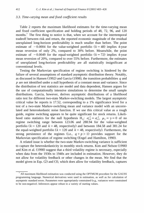
3.3. Time-Õarying mean and fixed coefficient results

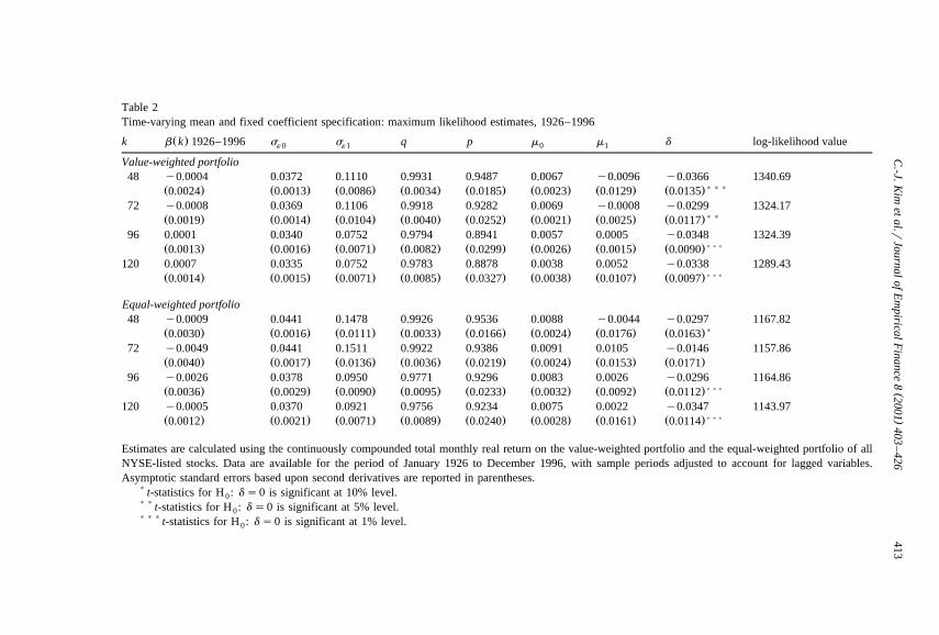
Table 2 reports the maximum likelihood estimates for the time-varying meanand fixed coefficient specification and holding periods of 48, 72, 96, and 120months.7 The first thing to notice is that, when we account for the intertemporaltradeoff between risk and return, the reported economic magnitude of the residualunexplained long-horizon predictability is much smaller than before. The point

Ž .estimate of y0.0004 for the value-weighted portfolio ks48 implies 4-yearmean reversion of only 2%, compared to 30% before. Meanwhile, the point

Ž .estimate of y0.0049 for the equal-weighted portfolio ks72 implies 4-yearmean reversion of 20%, compared to over 55% before. Furthermore, the estimatesof unexplained long-horizon predictability are all statistically insignificant atconventional levels.

Testing the Markovian specification of regime switching is hindered by thefailure of several assumptions of standard asymptotic distribution theory. Notably,

Ž . Ž .as discussed in Hansen 1992 and Garcia 1998 , the transition probabilities q andp are not identified under a null hypothesis of a constant mean and variance. Sincethe distribution of test statistics are model and data dependent, Hansen argues forthe use of computationally intensive simulations to determine the small sampledistributions. Garcia, however, derives asymptotic distributions of a likelihoodratio test for different two-state Markov-switching models. The largest asymptoticcritical value he reports is 17.52, corresponding to a 1% significance level for atest of a two-state Markov-switching mean and variance model with an uncorre-lated and heteroskedastic noise function. If we use this critical value as a roughguide, regime switching appears to be quite significant for stock returns. Likeli-hood ratio statistics for the null hypothesis H : s 2 ss 2 , m sgs0 of no0 ´ 0 ´1 1

regime switching range between 123.06 and 288.94 for the value-weightedŽ .portfolio ks120 and ks48, respectively and between 184.58 and 381.24 for

Ž .the equal-weighted portfolio ks120 and ks48, respectively . Furthermore, theŽ .strong persistence of the regimes i.e., qqp)1 provides support for the

Ž .Markovian specification of regime switching Engel and Hamilton, 1990 .A related issue is whether the two-state Markov-switching variance is sufficient

Ž .to capture the heteroskedasticity in monthly stock returns. Kim and Nelson 1998Ž .and Kim et al. 1998 suggest that a third volatility regime is necessary, especially

when data from the 1930s to 1940s are included in estimation. However, they donot allow for volatility feedback or other changes in the mean. We find that the

Ž . Ž .model given in Eqs. 2 and 3 , which does allow for volatility feedback, captures

7 All maximum likelihood estimation was conducted using the OPTMUM procedure for the GAUSSprogramming language. Numerical derivatives were used in estimation, as well as for calculation of

Žasymptotic standard errors. Parameters were appropriately constrained e.g., variances were constrained.to be non-negative . Inferences appear robust to a variety of starting values.

()

C.-J.K

imet

al.rJournalof

Em

piricalFinance

82001

403–

426413

Table 2Time-varying mean and fixed coefficient specification: maximum likelihood estimates, 1926–1996

Ž .k b k 1926–1996 s s q p m m d log-likelihood value´ 0 ´1 0 1

Value-weighted portfolio48 y0.0004 0.0372 0.1110 0.9931 0.9487 0.0067 y0.0096 y0.0366 1340.69

)))Ž . Ž . Ž . Ž . Ž . Ž . Ž . Ž .0.0024 0.0013 0.0086 0.0034 0.0185 0.0023 0.0129 0.013572 y0.0008 0.0369 0.1106 0.9918 0.9282 0.0069 y0.0008 y0.0299 1324.17

))Ž . Ž . Ž . Ž . Ž . Ž . Ž . Ž .0.0019 0.0014 0.0104 0.0040 0.0252 0.0021 0.0025 0.011796 0.0001 0.0340 0.0752 0.9794 0.8941 0.0057 0.0005 y0.0348 1324.39

)))Ž . Ž . Ž . Ž . Ž . Ž . Ž . Ž .0.0013 0.0016 0.0071 0.0082 0.0299 0.0026 0.0015 0.0090120 0.0007 0.0335 0.0752 0.9783 0.8878 0.0038 0.0052 y0.0338 1289.43

)))Ž . Ž . Ž . Ž . Ž . Ž . Ž . Ž .0.0014 0.0015 0.0071 0.0085 0.0327 0.0038 0.0107 0.0097

Equal-weighted portfolio48 y0.0009 0.0441 0.1478 0.9926 0.9536 0.0088 y0.0044 y0.0297 1167.82

)Ž . Ž . Ž . Ž . Ž . Ž . Ž . Ž .0.0030 0.0016 0.0111 0.0033 0.0166 0.0024 0.0176 0.016372 y0.0049 0.0441 0.1511 0.9922 0.9386 0.0091 0.0105 y0.0146 1157.86

Ž . Ž . Ž . Ž . Ž . Ž . Ž . Ž .0.0040 0.0017 0.0136 0.0036 0.0219 0.0024 0.0153 0.017196 y0.0026 0.0378 0.0950 0.9771 0.9296 0.0083 0.0026 y0.0296 1164.86

)))Ž . Ž . Ž . Ž . Ž . Ž . Ž . Ž .0.0036 0.0029 0.0090 0.0095 0.0233 0.0032 0.0092 0.0112120 y0.0005 0.0370 0.0921 0.9756 0.9234 0.0075 0.0022 y0.0347 1143.97

)))Ž . Ž . Ž . Ž . Ž . Ž . Ž . Ž .0.0012 0.0021 0.0071 0.0089 0.0240 0.0028 0.0161 0.0114

Estimates are calculated using the continuously compounded total monthly real return on the value-weighted portfolio and the equal-weighted portfolio of allNYSE-listed stocks. Data are available for the period of January 1926 to December 1996, with sample periods adjusted to account for lagged variables.Asymptotic standard errors based upon second derivatives are reported in parentheses.

) t-statistics for H : ds0 is significant at 10% level.0)) t-statistics for H : ds0 is significant at 5% level.0))) t-statistics for H : ds0 is significant at 1% level.0


most of the negative skewness and leptokurtosis in stock returns. In particular, theŽ .standardized residuals for Eq. 2 display much less heteroskedasticity than the

Ž . 8 Ž . 2Ž .residuals for Eq. 1 . The Jarque and Bera 1980 x 2 test statistics based onthe third and fourth sample moments fall from 734.57, 853.65, 215.26, and 214.58

Žto only 16.05, 14.84, 2.28, and 2.61 for the value-weighted portfolio ks48,.ks72, ks96, and ks120, respectively and from 1048.39, 1183.70, 361.89,

and 455.28 to only 10.96, 12.67, 19.16, and 28.27 for the equal-weighted portfolioŽ .ks48, ks72, ks96, and ks120, respectively . Meanwhile, further address-ing heteroskedasticity by adding a third volatility regime should only weaken theevidence of mean reversion for the unexplained price movements. Kim and NelsonŽ . Ž .1998 and Kim et al. 1998 find that the evidence of mean reversion for overallstock returns is much weaker when a three-state Markov-switching variancespecification is considered. Also, the more flexible the time-varying mean, themore likely it can spuriously explain predictable price movements. Our two-statespecification provides the minimal possible flexibility, while still allowing us totest our explanation of the reported mean reversion evidence.

Beyond the unexplained long-horizon predictability and the variance process,the estimates of m , m , and d , which correspond to the expected return and the0 1

volatility feedback effect, are also of considerable interest. Contrary to the findingsŽ .in Turner et al. 1989 , we find that the estimated partial effect m of an increase1

in expected volatility is actually positive in most cases, although it is neverstatistically significant.9 For the case that corresponds to strongest evidence of

Ž .mean reversion in Table 1 i.e., the equal-weighted portfolio with ks72 , themean return more than doubles from 0.91% in a perfectly anticipated low volatilityregime to 1.96% in a perfectly anticipated high volatility regime. Meanwhile, theestimated volatility feedback effect d of an unanticipated transition into a highvolatility regime on the mean return is always negative, corresponding to apositive tradeoff between volatility and expected returns. The t-statistics for thenull hypothesis H : ds0 of no volatility feedback are between y2.56 and y3.870

Ž .for the value-weighted portfolio ks72 and ks96, respectively and betweenŽy0.85 and y3.04 for the equal-weighted portfolio ks72 and ks120, respec-

.tively . In terms of economic magnitude, even the smallest point estimates suggest

8 Since we do not directly observe the true state, we use smoothed, or two-sided, probabilities as theŽ .best available estimate of the true state in order to calculate the standardized residuals for Eq. 2 . The

smoothed probabilities are conditional on all available returns and the maximum likelihood estimates ofthe hyper-parameters presented in Table 2. As a result of this substitution, our standardized residualsmay be less Normal than the true residuals. Also, it should be noted that, while the use of the smoothed

Ž . Ž .probabilities reduces the sample of standardized residuals for Eq. 2 , we compare residuals for Eqs. 1Ž .and 2 using the same adjusted sample periods.

9 Ž .Turner et al. 1989 find a negative, but insignificant, partial effect using excess returns fromStandard and Poor’s composite index for the sample period of January 1946 to December 1987.


that a completely unanticipated transition into a high volatility regime produces anŽ .immediate 2.99% decline in the value-weighted portfolio ks72 and an immedi-

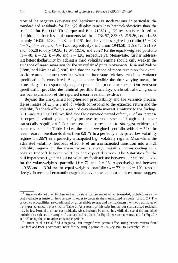
Ž .ate 1.46% decline in the equal-weighted portfolio ks72 .Fig. 1 displays the filtered and smoothed probabilities of a high volatility

regime for holding periods of 48, 72, 96, and 120 months. The filtered, orone-sided, probabilities are conditional on returns up to time t and maximumlikelihood estimates of the hyper-parameters presented in Table 2. The smoothed,or two-sided, probabilities are conditional on all available returns and the samemaximum likelihood estimates. The main thing to notice about the probabilities is

Ž .that, for both portfolios ks48 and ks72 , there are seemingly periodic3–4-year regime shifts during the 1930s and 1940s. While there are also regime

Fig. 1. Filtered and smoothed probabilities of a high volatility regime, 1926–1996.


shifts in the postwar period, they come at much less regular intervals. Given ourfinding that residual unexplained movements are largely unpredictable over longhorizons, this historical pattern of regime changes suggests that volatility regimechanges in 1930s and 1940s are responsible for the reported evidence of meanreversion. In particular, the timing of the tradeoff between risk and return in the1930s and 1940s should produce negative sample autocorrelations at horizons thatwill be easiest to detect for ks72 and ks96.10 Meanwhile, unlike with fads,there should be no systematic mean reversion in this scenario.11 A dramaticimplication, then, is that the apparent long-horizon predictability should disappearin the postwar period as the regime shifts become less regular. We use the constantmean and time-varying coefficient specification to test this implication and verifyour explanation of the reported mean reversion evidence.

3.4. Constant mean and time-Õarying coefficient results

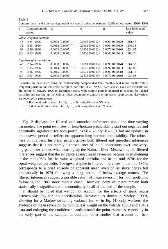
Table 3 reports maximum likelihood estimates for the constant mean andtime-varying coefficient specification and holding periods of 48, 72, 96, and 120months. The estimates for the variance of the time-varying parameter suggestchanges in the apparent long-horizon predictability of stock returns. The likelihoodratio statistics for the null hypothesis of constant predictability H : s 2s0 are as0 Õ

Ž . Ž .high as 4.3122 p-values0.038 for the value-weighted portfolio ks72 andŽ . Ž . 129.3183 p-values0.002 for the equal-weighted portfolio ks72 . These

results hold in spite of the fact that the maximum likelihood estimate of atime-varying parameter variance has a point mass at zero when the true variance is

Ž .small Stock and Watson, 1998 . Meanwhile, the estimates are generally consistentwith the Wald statistics reported in Table 1, while they avoid the problems,

Ž . Ž .discussed in Zivot and Andrews 1992 and Andrews 1993 , associated with anassumption of a known breakpoint.

10 As discussed previously, Jegadeesh tests with ks72 and ks96 are comparable to 3- and 4-yearŽ .overlapping autoregressions Richardson and Smith, 1994 .

11 Interestingly, given the Markov-switching specification, there should actually be some systematicmean aversion at shorter horizons. Heuristically, conditional on presently being in a high varianceregime, past and future returns are likely to be somewhat above average. However, this effect dies outas horizons get longer and conditional expectations revert to unconditional levels.

12 Although we report standard errors for all the parameters in the tables, we emphasize theŽ .likelihood ratio statistic for testing this hypothesis since Garbade 1977 shows that it has good finite

sample properties in detecting a variety of forms of parameter instability. To be clear, the likelihoodratio test does not have the highest local asymptotic power against specific forms of parameter

Ž .instability such as a random walk coefficient Nyblom, 1989 . However, our interest is in more generalforms of instability, as well as in the actual time path of the coefficient through time, which thetime-varying parameter approach provides. In addition, the asymptotic distribution of the likelihoodratio statistic is concentrated towards the origin under the null hypothesis, making the likelihood ratio

Žtest conservative in the sense that reported p-values understate the true level of significance Garbade,.1977; also see Kendall and Stuart, 1973 .


Table 3Constant mean and time-varying coefficient specification: maximum likelihood estimates, 1926–1996

k Adjusted sample s s m Log-likelihoodÕ ´

period value

Value-weighted portfolioŽ . Ž . Ž .48 1934–1996 0.0000 0.0004 0.0456 0.0012 0.0064 0.0012 1261.47

))Ž . Ž . Ž .72 1935–1996 0.0012 0.0007 0.0451 0.0012 0.0064 0.0013 1246.38Ž . Ž . Ž .96 1936–1996 0.0003 0.0007 0.0453 0.0012 0.0070 0.0016 1224.65Ž . Ž . Ž .120 1937–1996 0.0000 0.0001 0.0453 0.0012 0.0043 0.0021 1203.76

Equal-weighted portfolioŽ . Ž . Ž .48 1934–1996 0.0000 0.0002 0.0591 0.0015 0.0090 0.0014 1064.53

)))Ž . Ž . Ž .72 1935–1996 0.0014 0.0008 0.0575 0.0015 0.0097 0.0011 1066.00)))Ž . Ž . Ž .96 1936–1996 0.0015 0.0009 0.0572 0.0015 0.0095 0.0008 1051.18

Ž . Ž . Ž .120 1937–1996 0.0000 0.0001 0.0574 0.0015 0.0072 0.0016 1034.08

Estimates are calculated using the continuously compounded total monthly real return on the value-weighted portfolio and the equal-weighted portfolio of all NYSE-listed stocks. Data are available forthe period of January 1926 to December 1996, with sample periods adjusted to account for laggedvariables and starting up the Kalman filter. Asymptotic standard errors based upon second derivativesare reported in parentheses.

)) Likelihood ratio statistic for H : s s0 is significant at 5% level.0 Õ

))) Likelihood ratio statistic for H : s s0 is significant at 1% level.0 Õ

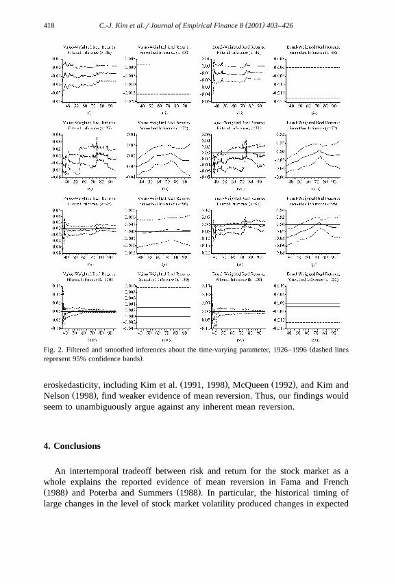
Fig. 2 displays the filtered and smoothed inferences about the time-varyingparameter. The point estimates of long-horizon predictability start out negative and

Ž .potentially significant for both portfolios ks72 and ks96 , but are updated inthe postwar period to reflect no apparent long-horizon predictability. The robust-ness of this basic historical pattern across both filtered and smoothed inferencessuggests that it is not merely a consequence of initial uncertainty over time-vary-ing parameter values when starting up the Kalman filter. Meanwhile, the filteredinferences suggest that the evidence against mean reversion became overwhelmingin the mid-1950s for the value-weighted portfolio and in the mid-1970s for theequal-weighted portfolio. The upward spike in filtered inferences in the mid-1970scorresponds to a brief episode of apparent mean aversion as stock prices felldramatically in 1974 following a long period of below-average returns. Thefiltered inferences suggest a possible return of mean reversion for both portfoliosfollowing the 1987 stock market crash. However, point estimates remain bothstatistically insignificant and economically small at the end of the sample.

It should be noted that we do not account for the effects of stock returnŽ .heteroskedasticity for this specification. However, as shown in Morley 1999 ,

Ž .allowing for a Markov-switching variance for ´ in Eq. 4 only weakens thet

evidence of mean reversion by putting less weight on the volatile 1930s and 1940sdata and enlarging the confidence bands around the point estimates, especially inthe early part of the sample. In addition, other studies that account for het-


ŽFig. 2. Filtered and smoothed inferences about the time-varying parameter, 1926–1996 dashed lines.represent 95% confidence bands .

Ž . Ž .eroskedasticity, including Kim et al. 1991, 1998 , McQueen 1992 , and Kim andŽ .Nelson 1998 , find weaker evidence of mean reversion. Thus, our findings would

seem to unambiguously argue against any inherent mean reversion.

4. Conclusions

An intertemporal tradeoff between risk and return for the stock market as awhole explains the reported evidence of mean reversion in Fama and FrenchŽ . Ž .1988 and Poterba and Summers 1988 . In particular, the historical timing oflarge changes in the level of stock market volatility produced changes in expected


returns responsible for the apparent tendency of price movements to be offset overlong horizons. Meanwhile, the absence of periodic changes in volatility during thepostwar period corresponds to a disappearance of any apparent long-horizonpredictability for the postwar data. We arrive at these conclusions in two ways.First, when we consider an empirical model of stock returns that captures volatilityfeedback in the presence of a positive tradeoff between market volatility andexpected returns, we find that residual unexplained price movements are largelyunpredictable over long horizons. Second, when we allow the apparent long-hori-zon predictability of stock returns to change over time with a time-varyingparameter model, we find that postwar price movements are more consistent withthe behaviour implicit in the historical tradeoff between risk and return than anysystematic mean reversion.

We conclude this paper by noting that our results provide strong support formarket efficiency. To be clear, we do not provide a decisive test of marketefficiency. In particular, had we been unable to explain the reported meanreversion evidence, we could easily have argued that our results were a conse-quence of a misspecification of equilibrium expected returns, rather than, say, afailure of market efficiency due to a systematic overreaction by investors to newsabout fundamentals. However, given that our measure of the intertemporal tradeoffbetween risk and return does explain the reported mean reversion evidence, theargument for a failure of market efficiency due to investor overreaction is largelydiscredited. First, we find no evidence of opportunities for arbitrage over longhorizons. Instead, the optimal forecast appears to be the same as the equilibriumexpected return implied by the intertemporal tradeoff between risk and return.Second, the most recent estimates of long-horizon predictability actually supportthe random walk hypothesis. That is, contrary to the implication of a systematicoverreaction by investors, postwar stock returns appear largely unpredictable overlong horizons given past returns.

Acknowledgements

We have received helpful comments from Charles Engel, Dick Startz, EricZivot, participants in seminars at the Federal Reserve Bank of Dallas, the FederalReserve Bank of St. Louis, Washington University, and the University of Wash-ington, and two anonymous referees, but responsibility for any errors is entirelyour own. Support from the National Science Foundation under grants SBR-9711301and SES-9818789 and the Ford and Louisa Van Voorhis endowment at theUniversity of Washington is gratefully acknowledged. This paper is based in part

Ž .on Morley’s 1999 doctoral dissertation at the University of Washington. Earlierdrafts of the paper circulated under the title ADo Changes in the Market RiskPremium Explain the Empirical Evidence of Mean Reversion in Stock Prices?B


A.1. Estimation of the time-varying mean and fixed coefficient specification

Ž . Ž .For the specification presented in Eqs. 2 and 4 , an extended version of theŽ .filter discussed in Hamilton 1989 is given by the following three steps.

Step 1a: Calculate the joint probability of S , S , S , and S)'Ýky1St ty1 tyk t js2 tyjw xand solve for Pr S s1Nr ,r , . . . by summing across all possible values oft ty1 ty2

S , S , and S) :ty1 tyk t

)Pr S s j,S s i ,S sh ,S smNr ,r , . . .t ty1 tyk t ty1 ty2

)w xsPr S s jNS s i PPr S s i ,S sh ,S smNr ,r , . . . ,t ty1 ty1 tyk t ty1 ty2

A.1Ž .

w xPr S s1Nr ,r , . . .t ty1 ty2

1 1 ky2)s Pr S s1,S s i ,S sh ,S smNr ,r , . . . .Ý Ý Ý t ty1 tyk t ty1 ty2

is0hs0ms0

A.2Ž .

Step 1b: Calculate the conditional density of r :t

f r NS s j,S s i ,S sh ,S)sm ,r ,r , . . .Ž .t t ty1 tyk t ty1 ty2

2k1 1) )s exp y r yb k r , A.3Ž . Ž .ÝS S2 t ty j2 ½ 5ž /2s2ps S( js1tSt

) w x Ž wwhere r ' r y m y m Pr S s 1 N r ,r , . . . y d S y Pr S s 1 Ns t 0 1 t ty1 ty2 t tt

x. )r ,r , . . . . Note that given data up to time t, S , S , S , S , andty1 ty2 t ty1 tyk tŽ .particular values for the parameters, we observe all the elements of Eq. A.3 since

k k)r s r ym PkÝ ÝS tyj 0ty j

js1 js1

k k

y m yd P Pr S s1Nr ,r , . . . yd SŽ . Ý Ý1 tyj tyjy1 tyjy2 tyjjs1 js1

and

k)S sS qS qS .Ý ty j ty1 t tyk

js1


Step 2: Calculate the joint density of r , S , S , S , and S) and collapset t ty1 ty k t

across all possible states to find the marginal density of r :t

f r ,S s j,S s i ,S sh ,S)smNr ,r , . . .Ž .t t ty1 tyk t ty1 ty2

s f r NS s j,S s i ,S sh ,S)sm ,r ,r , . . .Ž .t t ty1 tyk t ty1 ty2

= )Pr S s j,S s i ,S sh ,S smNr ,r , . . . , A.4Ž .t ty1 tyk t ty1 ty2

f r Nr ,r , . . .Ž .t ty1 ty2

1 1 1 ky2)s f r ,S s j,S s i ,S sh ,S smNr ,r , . . . .Ž .Ý Ý Ý Ý t t ty1 tyk t ty1 ty2

js0is0hs0ms0

A.5Ž .

Step 3: Update the joint probability of S , S , S , and S) given r andt ty1 ty k t t

solve for the joint probability of S , S , and S) :t tykq1 tq1

)Pr S s j,S s i ,S sh ,S smNr ,r , . . .t ty1 tyk t t ty1

f r ,S s j,S s i ,S sh ,S)smNr ,r , . . .Ž .t t ty1 tyk t ty1 ty2s , A.6Ž .

<f r r ,r , . . .Ž .t ty1 ty2

)Pr S s j,S sg ,S snNr ,r , . . .t tykq1 tq1 t ty1

1 1)s Pr S s j,S s i ,S sh ,S sg ,S snNr ,r , . . . ,Ý Ý t ty1 tyk tykq1 tq1 t ty1

is0hs0

A.7Ž .

where

)Pr S s j,S si ,S sh ,S sg ,S smNr ,r , . . .t ty1 tyk tykq1 t t ty1

sPr S shNS sgtyk tykq1

)=Pr S s j,S si ,S sh ,S smNr ,r , . . .t ty1 tyk t t ty1

)´Pr S s j,S si ,S sh ,S sg ,S snNr ,r , . . . ,t ty1 tyk tykq1 tq1 t ty1

since S) sS qS)yS .tq1 ty1 t tykq1w x ) w )

)Then, given Pr S s1 for i s0, . . . ,ky1 and Pr S s i,S sh,S syi 0 ykq1 1x Ž . Ž .m for is0,1, hs0,1, and ms0, . . . ,ky1, we iterate through Eqs. A.1 – A.7


w xfor ts1, . . . ,T to obtain the filtered probability Pr S s1Nr ,r , . . . . We uset ty1 ty2w x

)the unconditional probabilities for Pr S s1 :yi

1ypw x)Pr S s0 s , A.8Ž .yi 2ypyq

1yqw x)Pr S s1 s . A.9Ž .yi 2ypyq

w ) xAs for Pr S s i,S sh,S sm , deriving unconditional joint probabilities in0 ykq1 1

terms of q and p is impractical for large values of k. Instead, we treat these initialŽ . Ž .probabilities, denoted Ps p , . . . ,p , as 4= ky1 additional parameters1 4Žky1.

to be estimated.Ž .We use the marginal density of r given in Eq. A.5 to find maximumt

likelihood estimates of the parameters as follows:

T

maxl u s ln f r Nr ,r , . . . , A.10Ž . Ž . Ž .Ž .Ý t ty1 ty2u ts1

Ž . 13where us b ,s ,s ,q, p,m ,m ,d ,P .´ 0 ´1 0 1

In addition to making the above inferences, we also obtain the smoothedw x Ž .probability Pr S s1Nr ,r , . . . by employing Kim’s 1994 smoothing algo-t T Ty1

w xrithm. Specifically, given the filtered probability Pr S s jNr ,r , . . . , which cant t ty1Ž .be found by collapsing across states for Eq. A.7 , and the conditional probability

w x Ž .Pr S s jNr ,r , . . . , given in Eq. A.2 , we iterate backwards through thet ty1 ty2Žfollowing two equations conditional on S s j and S s l, where js0,1 andt tq1

.ls0,1 :

w xPr S s l ,S s jNr ,r , . . .tq1 tq1 T Ty1

w x w x w xPr S s lNr ,r , . . . PPr S s jNr ,r , . . . PPr S s lNS s jtq1 T Ty1 t t ty1 tq1 ts

w xPr S s lNr ,r , . . .tq1 t ty1

A.11Ž .1

w x w xPr S s jNr ,r , . . . s Pr S s l ,S s jNr ,r , . . . .Ýtq1 T Ty1 tq1 tq1 T Ty1ls0

A.12Ž .

13 Since we are not particularly interested in making inferences about the startup probabilities, we donot report their estimates. Also, for practical reasons, we treat their values as known for calculation ofasymptotic standard errors based upon second derivatives. We consider this approach reasonable sinceinferences about the other parameters are virtually identical for other startup probabilities such as anequal probability for each initial state.


A.2. Estimation of the constant mean and time-varying coefficient specifica-tion

Ž . Ž .For specification presented in Eqs. 4 and 5 , the Kalman filter is given by theŽ Ž . k .following six equations let b 'b k , y 'r ym and x 'Ý y :t t t t t js1 tyj

Prediction

b sb , A.13Ž .t N ty1 ty1N ty1

P sP qs 2 , A.14Ž .t N ty1 ty1N ty1 Õ

h 'y yy sy yb x , A.15Ž .t N ty1 t t N ty1 t t N ty1 t

f sx P xXqs 2 , A.16Ž .t N ty1 t t N ty1 t ´

Updating

b sb qK h , A.17Ž .t N t t N ty1 t t N ty1

P sP yK x P , A.18Ž .t N t t N ty1 t t t N ty1

w xwhere b 'E b Nr ,r , . . . , for example, is the conditional expectationt N ty1 t ty1 ty2

of b ; P is the variance of b ; f is the variance of h ; andt t N ty1 t N ty1 t N ty1 t N ty1

K 'P xX fy1 is the Kalman gain.14t t N ty1 t t N ty1

Ž . Ž .Given some initial values b and P , we iterate through Eqs. A.13 – A.180 N0 0 N0

for ts1, . . . ,T to obtain filtered inferences about b conditional on informationt

up to time t. Also, as a by-product of this procedure, we obtain h and f ,t N ty1 t N ty1Ž .which based on the prediction error decomposition Harvey, 1990 can be used to

find maximum likelihood estimates of the hyper-parameters as follows:

T T1 1y1max l u sy ln 2p f y h f h , A.19Ž . Ž . Ž .Ý Ýt N ty1 t N ty1 t N ty1 t N ty12 2u tstq1 tstq1

Ž .where us m,s ,s .´ Õ

Note that we ignore the first t observations in calculating the likelihoodfunction. Since we do not observe b , and it has no unconditional expectation0

Ž .under the random walk specification given in Eq. 5 , we must make an arbitraryŽguess as to its value and assign our guess an extremely large variance e.g.,

.b s0 and P 40 . We then use the first t observations to determine b0 N0 0 N0 t Ntand P , which we treat as the initial values in the Kalman filter for the purposest Nt

14 For a more general discussion of the Kalman filter and time-varying parameter models, as well asŽ . Ž .details on the derivation of the Kalman gain, refer to Hamilton 1994a,b and Kim and Nelson 1999 .


of maximum likelihood estimation.15 In practice, there is no exact rule as to whatvalue of t to use. Roughly speaking, we choose t such that the effects of ourarbitrary initial guess are minimized subject to including as much data in estima-tion as possible. The adjusted samples given in Table 3 reflect our choices for t .The reported estimates appear to be robust to larger values of t .

Finally, given b and P from the last iteration of the Kalman filter, weT NT T NT

iterate backwards through the following two equations in order to obtain smoothedinferences about b conditional on information up to time T :t

Smoothing

b sb qP Py1 b yb , A.20Ž . Ž .t NT t N t t N t tq1N t tq1NT tq1N t

P sP qP Py1 P yP PXy1 PX . A.21Ž . Ž .t NT t N t t N t tq1N t tq1NT tq1N t tq1N t t N t

A.3. Calculation of mean reversion following a price shock

We measure the economic significance of parameter estimates by calculatingthe implied mean reversion of a price shock over a 4-year horizon. That is, wecalculate the cumulative effect of a shock on j-period-ahead return forecasts,where js1, . . . ,48 months. Construction of a given j-period-ahead forecast issomewhat complicated for the Jegadeesh regression equation. Specifically, follow-

Ž .ing Doan et al. 1984 , we need to employ an iterative procedure to calculatemulti-period forecasts given a 1-month dependent variable. For the first specifica-tion, the law of iterated expectations implies that the resulting forecast representsw j xE Ý r Nr ,r , . . . . However, it should be noted that the law of iteratedis1 tqi t ty1

expectations does not apply for the extensions since multi-period forecasts arenonlinear functions of past information.

The iterative approach to calculating economic significance works as follows.First, at time t, there is a one-unit shock. Then, for kG48 and jF48, thej-period-ahead expected demeaned return is calculated recursively for js1, . . . ,48

ˆŽ .months by r ymsb k R , where R s1 and, more generally, Rˆtq jN t tqjy1N t t tqjy1jy1Ž .'1qÝ r ym is the cumulative effect of a one-unit shock over a jy1ˆis1 tqiN t

ˆŽ .period horizon, with m and b k representing point estimates of the parameters.ˆFinally, the 4-year mean reversion following the initial shock is given byR y1.tq48N t

15 Alternatively, we could treat the initial value as a hyper-parameter to be estimated by maximumlikelihood estimation. Inferences are very similar in both cases. However, since the hyper-parametersare treated as known, the standard error bands surrounding the inferences in this alternative case woulddramatically understate the true degree of uncertainty during the early part of the sample. This isprecisely when our uncertainty should be greatest.


References

Andrews, D.W.K., 1993. Tests for parameter instability and structural change with unknown changepoint. Econometrica 61, 821–856.

Campbell, J.Y., Hentschel, L., 1992. No news is good news: an asymmetric model of changingvolatility in stock returns. Journal of Financial Economics 31, 281–318.

Campbell, J.Y., Shiller, R., 1988. The dividend–price ratio and expectations of future dividends anddiscount factors. Review of Financial Studies 1, 195–227.

Cecchetti, S.G., Lam, P., Mark, N.C., 1990. Mean reversion in equilibrium asset prices. AmericanEconomic Review 80, 398–418.

Doan, T., Litterman, R.B., Sims, C.A., 1984. Forecasting and conditional projection using realisticprior distributions. Econometric Reviews 3, 1–100.

Engel, C., Hamilton, J.D., 1990. Long swings in the dollar: are they in the data and do markets knowit? American Economic Review 80, 689–713.

Engle, R.F., Watson, M., 1987. Kalman filter: applications to forecasting and rational-expectationmodels. Advances in Econometrics, Fifth World Congress, vol. 1, pp. 245–281.

Fama, E.F., French, K.R., 1988. Permanent and temporary components of stock prices. Journal ofPolitical Economy 96, 246–273.

French, K.R., Schwert, G.W., Stambaugh, R.F., 1987. Expected stock returns and volatility. Journal ofFinancial Economics 19, 3–29.

Garbade, K., 1977. Two methods for examining the stability of regression coefficients. Journal of theAmerican Statistical Association 72, 54–63.

Garcia, R., 1998. Asymptotic null distribution of the likelihood ratio test in Markov switching models.International Economic Review 39, 763–788.

Hamilton, J.D., 1989. A new approach to the economic analysis of nonstationary time series and thebusiness cycle. Econometrica 57, 357–384.

Hamilton, J.D., 1994a. Time Series Analysis. Princeton Univ. Press.Ž .Hamilton, J.D., 1994b. State-space models. In: Engle, R.F., McFadden, D.L. Eds. , 1994b. Handbook

of Econometrics, vol. 4, North-Holland, Amsterdam, pp. 3014–3077.Hamilton, J.D., Susmel, R., 1994. Autoregressive conditional heteroskedasticity and changes in regime.

Journal of Econometrics 64, 307–333.Hansen, B.E., 1992. The likelihood ratio test under nonstandard conditions: testing the Markov

switching model of GNP. Journal of Applied Econometrics 7, S61–S82.Harvey, A.C., 1990. The Econometric Analysis of Time Series. 2nd edn. MIT Press, Cambridge.Jarque, C., Bera, A., 1980. Efficient tests for normality, heteroskedasticity, and serial independence of

regression residuals. Economics Letters 6, 255–259.Jegadeesh, N., 1991. Seasonality in stock price mean reversion: evidence from the U.S. and the U.K.

Journal of Finance 46, 1427–1444.Kendall, M., Stuart, A., 1973. 3rd edn. The Advanced Theory of Statistics, vol. 2, Hafner Publishing,

New York.Kim, C.-J., 1994. Dynamic linear models with Markov-switching. Journal of Econometrics 60, 1–22.Kim, C.-J., Nelson, C.R., 1998. Testing for mean reversion in heteroskedastic data II: autoregression

tests based on Gibbs-sampling-augmented randomization. Journal of Empirical Finance 5, 385–396.Kim, C.-J., Nelson, C.R., 1999. State-Space Models with Regime Switching: Classical and Gibbs-Sam-

pling Approaches with Applications. MIT Press, Cambridge.Kim, C.-J., Nelson, C.R., Startz, R., 1998. Testing for mean reversion in heteroskedastic data based on

Gibbs-sampling-augmented randomization. Journal of Empirical Finance 5, 131–154.Kim, C.-J., Morley, J.C., Nelson, C.R., 2001, Is there a positive relationship between stock market

volatility and the equity premium? Manuscript, Washington University.Kim, M.-J., Nelson, C.R., Startz, R., 1991. Mean reversion in stock prices? A reappraisal of the

empirical evidence. Review of Economic Studies 48, 515–528.


Maheu, J.M., McCurdy, T.H., 2000. Identifying bull and bear markets in stock returns. Journal ofBusiness and Economic Statistics 18, 100–112.

Mayfield, E.S., 1999. Estimating the market risk premium, Manuscript, Harvard Business School.McQueen, G., 1992. Long-horizon mean-reverting stock prices revisited. Journal of Financial and

Quantitative Analysis 27, 1–18.Morley, J.C., 1999. Essays in empirical finance, PhD dissertation, University of Washington.Nyblom, J., 1989. Testing for the constancy of parameters over time. Journal of the American

Statistical Association 84, 223–230.Officer, R.R., 1976. The variability of the market factor of the New York Stock Exchange. Journal of

Business 46, 434–453.Poterba, J.M., Summers, L.H., 1988. Mean reversion in stock prices: evidence and implications.

Journal of Financial Economics 22, 27–59.Richardson, M., 1993. Temporary components of stock prices: a skeptic’s view. Journal of Business

and Economic Statistics 11, 199–207.Richardson, M., Smith, T., 1994. A unified approach to testing for serial correlation in stock returns.

Journal of Business 67, 371–399.Richardson, M., Stock, J.H., 1989. Drawing inferences from statistics based on multiyear asset returns.

Journal of Financial Economics 25, 323–348.Schaller, H., van Norden, S., 1997. Regime switching in stock market returns. Applied Financial

Economics 7, 177–191.Schwert, G.W., 1989a. Business cycles, financial crises, and stock volatility. Carnegie-Rochester

Conference Series on Public Policy 31, 83–126.Schwert, G.W., 1989b. Why does stock market volatility change over time? Journal of Finance 44,

1115–1153.Stock, J.H., Watson, M.W., 1998. Median unbiased estimation of coefficient variance in a time-varying

parameter model. Journal of the American Statistical Association 93, 349–358.Summers, L.H., 1986. Does the stock market rationally reflect fundamental values? Journal of Finance

41, 591–601.Turner, C.M., Startz, R., Nelson, C.R., 1989. A Markov model of heteroskedasticity, risk, and learning

in the stock market. Journal of Financial Economics 25, 3–22.White, H., 1980. A heteroskedasticity-consistent covariance matrix estimator and a direct test for

heteroskedasticity. Econometrica 48, 817–838.Zivot, E., Andrews, D.W.K., 1992. Further evidence on the great crash, the oil price shock, and the

unit root hypothesis. Journal of Business and Economic Statistics 10, 251–270.

Does an intertemporal tradeoff between risk and...

Documents

Transcript of Does an intertemporal tradeoff between risk and...