DOCUMENTS DE TREBALL

DE LA FACULTAT D’ECONOMIA I EMPRESA

Col.lecció d’Economia

E12/284

Educational expansion, intergenerational mobility and over-education**

Montserrat Vilalta-Bufí* Departament de Teoria Econòmica i CREB (Universitat de Barcelona)

Ausias Ribó Departament de Teoria Econòmica i CREB (Universitat de Barcelona)

* Corresponding author: Montserrat Vilalta-Bufí, Departament de Teoria Econòmica; Universitat de Barcelona, Avda. Diagonal 690; 08034 Barcelona; Spain. E-mail: montsevilalta@ub.edu; tel: (+34)934020107; Fax: (+34) 934039082. ** The authors are grateful to the Spanish Ministry of Education for financial support through the grant ECO2012-34046 and to the Government of Catalonia through the Barcelona GSE Research Network and grant 2009SGR1051.

Abstract

There is a vast literature on intergenerational mobility in sociology and economics. Similar

interest has emerged for the phenomenon of over-education in both disciplines. There are no

studies, however, linking these two research lines. We study the relationship between social

mobility and over-education in a context of educational expansion. Our framework allows for

the evaluation of several policies, including those a¤ecting social segregation, early intervention

programs and the power of unions. Results show the evolution of social mobility, over-education,

income inequality and equality of opportunity under each scenario.

Keywords: good jobs, intergenerational cultural transmission, aggregate productivity, match-ing model, over-education

J.E.L. Classi�cation Code:. J21, J24, J62, I24

Resum:

Hi ha una àmplia literatura sobre la mobilitat intergeneracional a les àrees de sociologia i

economia. El fenomen de la sobreeducació ha suscitat interès similar en ambdues disciplines. No

hi ha estudis, però, que uneixin aquestes dues línies d�investigació. En aquest article s�estudia

la relació entre la mobilitat social i la sobre-educació en un context d�expansió de l�educació. El

nostre marc permet l�avaluació de diverses polítiques, com les que afecten la segregació social, els

programes d�intervenció primerenca i el poder dels sindicats. Els resultats mostren l�evolució de

la mobilitat social, la sobre-educació, la desigualtat i la igualtat d�oportunitats en cada escenari.

Paraules clau: transmissió cultural, mobilitat intergeneracional, funció de matching, sobre-educació.

Classi�cació JEL: J21, J24, J62, I24

1 Introduction

There is a vast literature on inter-generational mobility (see reviews of the empirical literature

in Solon, 1999; Björklund and Jäntti, 2009 and Black and Devereux, 2011). Social mobility

is often studied in relationship to the process of development, wealth distribution, inequality

and economic growth. These variables are usually linked via individuals�investment decisions

in education and its return. Education is positively related to development and growth and

explains at least partially wealth distribution and inequality. The cost of education is commonly

de�ned in monetary terms and the introduction of some type of capital market imperfections

explain why kids from poor families have less access to education than kids from richer families

(Becker and Tomes, 1986; Galor and Tsiddon, 1997; Loury, 1981; Maoz and Moav, 1999).1

Lefgren, Lindquist and Sims (2012), however, estimate that no more than 37 percent of the

income persistence between fathers and sons is attributable to the causal e¤ect of �nancial

resources. Therefore, there is room for other mechanisms to explain the persistence in income

across generations.

The so called �mechanistic persistence�refers to the transmission of human capital indepen-

dently of the level of �nancial investment. It includes the transmission of genetic traits and

other non-�nancial investments. Understanding the transmission mechanisms in place is crucial

to develop e¤ective policies to improve equality of opportunities and social mobility. Income

redistribution might be useful if �nancial constraints are binding (Benabou, 2002), but they

might be futile otherwise. Mayer (2008), for instance, assumes the presence of heterogeneous

abilities, which are transmitted across generations, generating a positive correlation between

fathers�and sons�incomes via self-selection into education. Early childhood intervention pro-

grams to improve ability of children from low-income families would then lead to better results

than subsidizing college education.

Our paper proposes a cultural transmission mechanism similar to the one proposed in Bisin

and Verdier (2001). Both direct parental e¤ort in terms of time devoted to children and social-

ization with neighbors a¤ect the probability of the kid to obtain high education. Several papers

provide empirical evidence on the importance of early parental attention (Heckman, Pinto and

Savelyev, 2012; Restuccia and Urrutia, 2004;) and neighborhood e¤ects (Case and Katz, 1991;

O�Regan and Quigley, 1996; Cutler and Glaeser, 1997) on kids�future educational outcomes.

We combine the cultural transmission of education with the presence of frictions in the

labor market. This allows us to introduce another phenomenon in the analysis of social mo-

bility: over-education. Over-education occurs when individuals� job require a lower level of

1An exception is Galor and Tsiddon (1997), who study the e¤ect of technological progress on intergenerational

mobility under the assumption of perfect capital markets. Technological progress increases incentives to invest

in education overtime, leading to higher mobility. We di¤er from them in that we do not include technological

progress, but cultural transmission of education and frictions in the labor market.

1

education than the one acquired. It is a consequence of the fast educational expansion that

occurred in most developed countries during last decades and it has been studied since the

late 70s�(Brunello, Garibaldi, and Wasmer, 2007; Freeman, 1976; Sicherman and Galor, 1990;

Kalleberg and Sorensen, 1979). There are no studies, however, linking over-education and inter-

generational mobility. We study the relationship between social mobility and over-education in

a context of educational expansion. Our framework allows for the evaluation of several policies,

including those a¤ecting social segregation, early intervention programs and the power of unions.

The paper is organized as follows. In the next section we develop the theoretical model,

which comprises of three main parts: the education transmission mechanism, the job allocation

process and the individual�s problem. In section 3 we �rst de�ne the variables of interest to

then perform several policy evaluations using simulation techniques. Finally, section 4 concludes

giving directions for further research.

2 The Model

We set up two initially independent mechanisms in our model. One refers to the educational

attainment of the population and the other explains how individuals get allocated to jobs. Then

we study how the interaction of these two mechanisms determines several measures of interest of

a country. These measures include the level of social mobility, over-education, income inequality

and aggregate productivity level.

The �rst mechanism consists on the transmission of education from parents to children. This

is thought to occur as the inter-generational cultural transmission in Bisin and Verdier (2001)

adapted to the transmission of education. We follow Patacchini and Zenou (2011). All parents

prefer high education for their kids. With some probability they succeed in transmitting their

preferences, otherwise children get the education level of a random individual of the population.

We depart from any capital market imperfections story or wealth transmission since these e¤ects

have been already widely analyzed in the literature (Becker and Tomes, 1986; Galor and Tsiddon,

1997; Loury, 1981; Maoz and Moav, 1999).

The second mechanism in our model explains how individuals get allocated to jobs using a

simple matching model. The number of good jobs is endogenously determined as well as the

productivity level. Moreover, individuals with parents in a good job are more likely to �nd a good

job than those individuals whose parents have a bad job. This is related to the fast expanding

literature on networks, that emphasizes the importance of having the right connections to obtain

the right information (Corak and Piraino, 2011; Ioannides and Loury, 2004).

We study the steady state equilibrium as well as transition dynamics, which are very relevant

since transition might take several generations.

2

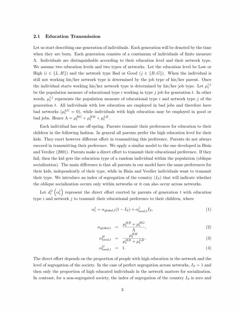
2.1 Education Transmission

Let us start describing one generation of individuals. Each generation will be denoted by the time

when they are born. Each generation consists of a continuum of individuals of �nite measure

�. Individuals are distinguishable according to their education level and their network type.

We assume two education levels and two types of networks. Let the education level be Low or

High (i 2 fL;Hg) and the network type Bad or Good (j 2 fB;Gg). When the individual isstill not working his/her network type is determined by the job type of his/her parent. Once

the individual starts working his/her network type is determined by his/her job type. Let �i;jtbe the population measure of educational type i working in type j job for generation t. In other

words, �i;jt represents the population measure of educational type i and network type j of the

generation t. All individuals with low education are employed in bad jobs and therefore have

bad networks (�LGt = 0), while individuals with high education may be employed in good or

bad jobs. Hence � = �HGt + �HBt + �LBt .

Each individual has one o¤-spring. Parents transmit their preferences for education to their

children in the following fashion. In general all parents prefer the high education level for their

kids. They exert however di¤erent e¤ort in transmitting this preference. Parents do not always

succeed in transmitting their preference. We apply a similar model to the one developed in Bisin

and Verdier (2001). Parents make a direct e¤ort to transmit their educational preference. If they

fail, then the kid gets the education type of a random individual within the population (oblique

socialization). The main di¤erence is that all parents in our model have the same preferences for

their kids, independently of their type, while in Bisin and Verdier individuals want to transmit

their type. We introduce an index of segregation of the country (IS) that will indicate whether

the oblique socialization occurs only within networks or it can also occur across networks.

Let dijt��jt

�represent the direct e¤ort exerted by parents of generation t with education

type i and network j to transmit their educational preference to their children, where

�jt = �global;t(1� IS) + �jlocal;tIS ; (1)

�global;t =�HBt + �HGt

�; (2)

�Blocal;t =�HBt

�HBt + �LBt; (3)

�Glocal;t = 1: (4)

The direct e¤ort depends on the proportion of people with high education in the network and the

level of segregation of the society. In the case of perfect segregation across networks, IS = 1 and

then only the proportion of high educated individuals in the network matters for socialization.

In contrast, for a non-segregated society, the index of segregation of the country IS is zero and

3

�jt corresponds to the proportion of highly educated individuals in the whole population. We

also allow for intermediate levels of segregation, IS 2 [0; 1].

Whether dijt(�jt ) is increasing or decreasing in �

jt will tell us whether direct and oblique

socialization are complementaries or substitutes. Pattachini and Zenou (2011) estimate this

relationship for the UK and �nd that neighborhood and parental involvement in kids education

are complementary.

The direct e¤ort exerted by parents translates into a probability of success in direct socializa-

tion, de�ned by the function f . Let this probability of success depend on the direct e¤ort exerted

by parents, d; and the proportion of high educated individuals, �jt , that is, fi(dijt(�

jt ); �

jt ).

We assume that f i(0; �) = 0, that is, without e¤ort there is no direct socialization. The

function f is increasing in e¤ort d and �. This means that higher e¤ort by parents increases the

probability of success in transmitting their preferences and given a level of e¤ort, having better

neighborhood translates into higher probability of success in direct socialization. We assume

therefore some kind of spillovers in the direct socialization process. Spillovers are needed in

order to allow for complementarity between direct and oblique socialization.

Based on the empirical evidence in Guryan, Hurst and Kearney (2008) and Patacchini and

Zenou (2011) we assume that parents with low education have lower quality direct e¤ort than

high education individuals.

fL(dLjt(�jt ); �

jt ) = �f

H(dHjt(�jt ); �

jt ) (5)

where � < 1:

We assume that the probability of oblique socialization is an increasing and convex function

on the proportion of highly educated individuals in the society.2 Let�s denote g(�jt ) the proba-

bility of oblique socialization. g(:) is such that g0 > 0 and g00 > 0. This implies that there is a

reinforcing e¤ect of having more educated individuals in the society. Increasing the proportion

of human capital has a stronger e¤ect on the probability of socialization when there are already

many highly educated individuals. Moreover, if everybody has high education, then oblique

socialization is successful with certainty, g(1) = 1.

Then the probabilities of education transition are the following:

�iHjt+1 = f i(dijt(�jt ); �

jt ) + (1� f i(dijt(�

jt ); �

jt ))g(�

jt ); (6)

�iLjt+1 = (1� f i(dijt(�jt ); �

jt ))(1� g(�

jt )): (7)

�iHjt+1 is the probability of a parent with education i and network j to transmit his/her

preference for high education to his/her kid. It has two components, the probability of success in

2This assumption is needed in order to obtain an interior equilibrium (or equivalently, a non-degenerate

population distribution).

4

direct transmission plus the probability of success in oblique socialization if direct transmission

fails. �iLjt+1 represents the probability of a parent with education i and network j to fail to

transmit the high education to the kid. This happens in the event of failure in direct and

oblique transmission.

Given these transition probabilities, we can �nd the measure of young individuals for each

type of education and network. Let ijt+1 be the measure of young individuals with education

type i and network type j just before entering the labor market. Recall that the network type

of this individuals is determined by the job type of their parents.

Lt+1 = �LLt+1�LBt +�HLB;t+1�

HBt +�HLG;t+1�

HGt ; (8)

HBt+1 = �LHt+1�LBt +�HHB;t+1�

HBt ; (9)

HGt+1 = �HHG;t+1�HGt : (10)

or in matrix notation:264 Lt+1 HBt+1 HGt+1

375 =264 �

LLt+1 �HLB;t+1 �HLG;t+1

�LHt+1 �HHB;t+1 0

0 0 �HHG;t+1

375264 �LBt�HBt�HGt

375 :Once the education transmission is completed we observe three types of children. Next we

study how this young individuals, given their education and network type, are allocated to jobs.

2.2 Job allocation

Let us now describe the labor demand. As already mentioned above, there are two types of job:

good and bad. A job exists when a suitable worker �lls a vacancy created by a �rm. Each �rm

can open only one vacancy. The vacancy cost is � > 0 for a good job and 0 for a bad job. Firms

are expected pro�t maximizers and there is free entry. Whereas there are search frictions in

the market for good jobs, the market for bad jobs is assumed perfectly competitive. Therefore,

everybody can instantly �nd a bad job and there are as many bad jobs as required. On the

other hand, the matching of highly educated individuals to good vacancies is not without e¤ort.

Individuals must search in order to �nd a good vacancy. The total number of good jobs created

is determined by a matching function m(ut; vt), where vt denotes the number of good vacancies

opened and ut denotes the total e¢ ciency units of search devoted to the good job market (as in

Bentolila, Michelacci and Suarez, 2008).

Similar to Bentolila et al (2008) we normalize to one the maximum e¢ ciency units of search

for a good job that an individual can use including formal channels (employment agencies,

newspaper adds, internet search, etc.) and networks. Each individual has access to a fraction of

this maximum e¢ ciency units of search. We assume that young individuals whose parents are in

5

good jobs have better networks than young individuals with parents in bad jobs. Therefore, the

former are endowed with a larger fraction of e¢ ciency units of search than the latter. In other

words, the network type is associated with di¤erent endowments of e¢ ciency units of search, S

for type G, s for type B with 1 � S > s > 0. Therefore, the total e¢ ciency units of search inthe good jobs market is ut = S HGt + s HBt .

Assume that the matching function for the good job,m(u; v); is increasing in both arguments,

continuous function and upper bounded by Minfut; vtg.3

Denote the production obtained in a bad job by yB;t and the production in a good job by

yG;t. The production of the bad job is given entirely to the worker as wage. In contrast, in

the good job, workers and �rms negotiate under a Nash bargaining game. The solution is that

each player gets a proportion of the total surplus created by a good match, which is yG;t� yB;t,plus the outside option. Let workers power be represented by �. Then the wage of a worker

employed in a good job is wGt = � (yG;t � yB;t) + yB;t. The following condition ensures that allindividuals with high education prefer a good job rather than a bad job:

spwGt > yB;t; (11)

where p = m(ut;vt)ut

2 [0; 1] is the probability per e¢ ciency unit of search to �nd a good job.Notice that the number of realized matches corresponds to the number of individual with high

education in a good job, �HGt = m(ut; vt).

The production function in each sector is assumed to have the following speci�cation:

yG;t = At�"global;t = At

��HBt + �HGt

�

�";

yB;t = At��Blocal;t

�"= At

��HBt

�� �HGt

�"; (12)

where " < 1 and At represents the productivity level. Notice that with this speci�cation of the

production function we are assuming that production of a good job depends on the proportion of

highly educated individual in the whole population, meanwhile production of a bad job depends

on the proportion of highly educated people in the bad job holders. It follows that yG;t > yB;t.

We assume free entry of �rms, and hence, �rms will open new vacancies in the good jobs

market until the expected pro�t of opening a vacancy equals its cost:4

q(1� �) (yG;t � yB;t) = �: (13)

where q = m(ut;vt)vt

2 [0; 1] is the probability for a �rm of getting a vacancy �lled.

3Ribo and Vilalta-Bu� (2012) analyze which properties are necessary for particular matching functions to be

bounded from above by the number of search units and vacancies.4To be precise, by the expected pro�t of opening a vacancy we mean the proportion of the expected surplus

generated by the creation of a new job that goes to the �rm.

6

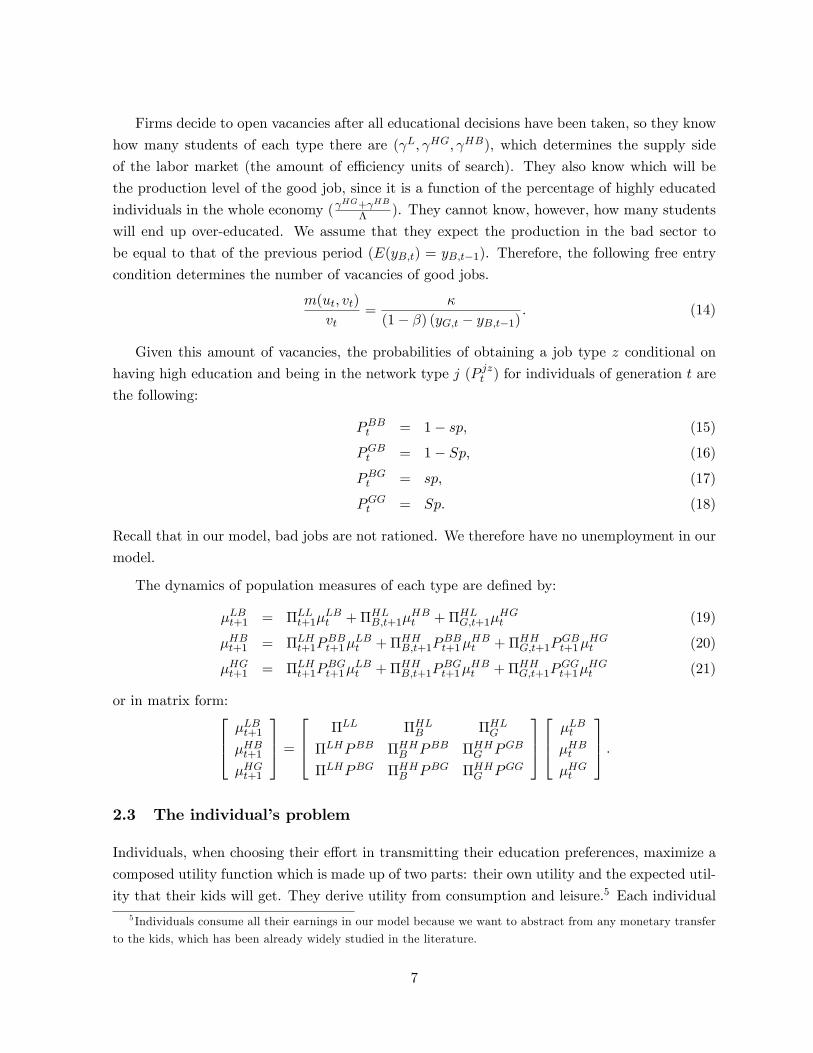
Firms decide to open vacancies after all educational decisions have been taken, so they know

how many students of each type there are ( L; HG; HB), which determines the supply side

of the labor market (the amount of e¢ ciency units of search). They also know which will be

the production level of the good job, since it is a function of the percentage of highly educated

individuals in the whole economy ( HG+ HB

� ). They cannot know, however, how many students

will end up over-educated. We assume that they expect the production in the bad sector to

be equal to that of the previous period (E(yB;t) = yB;t�1). Therefore, the following free entry

condition determines the number of vacancies of good jobs.

m(ut; vt)

vt=

�

(1� �) (yG;t � yB;t�1): (14)

Given this amount of vacancies, the probabilities of obtaining a job type z conditional on

having high education and being in the network type j (P jzt ) for individuals of generation t are

the following:

PBBt = 1� sp; (15)

PGBt = 1� Sp; (16)

PBGt = sp; (17)

PGGt = Sp: (18)

Recall that in our model, bad jobs are not rationed. We therefore have no unemployment in our

model.

The dynamics of population measures of each type are de�ned by:

�LBt+1 = �LLt+1�LBt +�HLB;t+1�

HBt +�HLG;t+1�

HGt (19)

�HBt+1 = �LHt+1PBBt+1�

LBt +�HHB;t+1P

BBt+1�

HBt +�HHG;t+1P

GBt+1�

HGt (20)

�HGt+1 = �LHt+1PBGt+1�

LBt +�HHB;t+1P

BGt+1�

HBt +�HHG;t+1P

GGt+1�

HGt (21)

or in matrix form:264 �LBt+1�HBt+1�HGt+1

375 =264 �LL �HLB �HLG�LHPBB �HHB PBB �HHG PGB

�LHPBG �HHB PBG �HHG PGG

375264 �LBt�HBt�HGt

375 :2.3 The individual�s problem

Individuals, when choosing their e¤ort in transmitting their education preferences, maximize a

composed utility function which is made up of two parts: their own utility and the expected util-

ity that their kids will get. They derive utility from consumption and leisure.5 Each individual5 Individuals consume all their earnings in our model because we want to abstract from any monetary transfer

to the kids, which has been already widely studied in the literature.

7

is endowed with 1 unit of leisure and has to decide how much of it will be devoted to him/herself

and how much will be devoted to the kid. The time devoted to the kid corresponds to the direct

e¤ort of socialization. There is empirical evidence that supports the idea that parental care of

the kid is a determinant of the future education level and other socioeconomic variables of the

kid (Heckman, Pinto and Savelyev, 2012; Restuccia and Urrutia, 2004).

When parents decide how much time to invest in educating their kids, they do not know the

salaries their kids will get. We assume their best guess is to consider they will face the same

situation as in their generation. Moreover, we assume that they do not take into account the

e¤ect of their decision in the aggregate outcome of the economy.

Then, the problem that parents of education i; having a job j have to solve is

Maxflijt ;d

ijt g

wt + u(lijt ; d

ijt ) + �

iHjt+1Et(V

iHjt+1) + �

iLjt+1Et(V

iLjt+1)

subject to wt = yB;t + ki=G� (yG;t � yB;t) ;lijt = 1� d

ijt ;

where dijt and lijt is how much of leisure is devoted to children and to oneself respectively and

Et(ViLj;t+1) = Et(w

LBt+1) = yB;t;

Et(ViHj;t+1) = Et(w

Hjt+1) = yB;t + P

jGt � (yG;t � yB;t) ;

�iHjt+1 = f i(dijt ; �jt ) + (1� f i(d

ijt ; �

jt ))g(�

jt );

�iLjt+1 = (1� f i(dijt ; �jt ))(1� g(�

jt )):

Here, we are assuming that parents do not take into account the future cost of socializing

children that their kids will have to bear. Parents control variable is the time investment in

education, dt.

The �rst order condition to the general problem is the following:

�u1 + u2 +@f i

@d(1� g(�jt ))Et(V iHt+1 � V iLt+1) = 0: (22)

Notice here that since u1 > 0 and@f i

@d > 0; we have that u1 > u2 in an interior equilibrium.

The economic interpretation of the �rst order condition is that the marginal cost of spending

time with the kid (which is the lost utility of leisure) must be equal to the bene�t of spending

time with the kid (the utility/disutility you get from spending time with the kid plus the increase

in expected utility of your kid).

The second order condition to the general problem is:

u11 � 2u12 + u22 +@2f i

@d2(1� g(�jt ))Et(V iHt+1 � V iLt+1) < 0: (23)

8

We assume a negative SOC in order to ensure that there is a maximum and the problem is

well de�ned. We assume satiation in leisure (u11 < 0).

Using the implicit function theorem we can check whether there is complementarity or sub-

stitutability between direct e¤ort and quality of the society.

@dt

@�jt=�h@2f i

@d@�jt(1� g(�jt ))�

@f i

@d g0(�jt )

iEt(V

iHt+1 � V iLt+1)

u11 � 2u12 + u22 + @2f i

@d2(1� g(�jt ))Et(V iHt+1 � V iLt+1)

: (24)

Proposition 1. If @2f i

@d@�jt(1 � g(�jt )) >

@f i

@d g0(�jt ), then there is complementarity between

direct e¤ort and oblique socialization. That is, @dt@�jt

> 0. If @2f i

@d@�jt(1 � g(�jt )) <

@f i

@d g0(�jt ), then

there is substitutability between direct e¤ort and oblique socialization. That is, @dt@�jt

< 0.

Notice that for the case f i�dijt ; �

jt

�= dijt , we have only substitutability between direct e¤ort

and �jt .

Notice that these conditions involve d and �. Therefore, depending on the values d and

� (endogenous to the model) we will observe substitutability or complementarity between di-

rect and oblique socialization. Moreover, an economy may change from one state to the other

overtime.

To allow for the possibility of complementarity, we need that the marginal e¤ect of e¤ort on

f is higher on societies with higher �. That is, given two societies with di¤erent proportion of

highly educated people whose citizens exert exactly the same level of e¤ort in educating kids, the

society with higher proportion of educated parents will have a higher marginal e¤ect of e¤ort.

In words of Bisin and Verdier (p.308): "direct socialization is in this case more e¢ cient, other

things equal, when the trait to be transmitted is held by a majority of the population, and hence

when oblique transmission is more e¢ cient". For getting complementarity of direct and oblique

socialization we need a minimum level of these spillovers.

2.4 Timing

Let us summarize the model by stating clearly the timing within each period. The economy

starts with an initial distribution of the population: �LBt ; �HBt ; �HGt . This initial condition

determines the production level of good and bad jobs in this period. Each individual decides

how much direct e¤ort to exert given initial conditions and their expectations, which we assume

that are determined based on the initial conditions. These decisions on direct e¤ort plus the

process of oblique socialization give as an outcome the distribution of young individuals for next

generation: Lt+1; HBt+1 ;

HGt+1.

9

Once the distribution of young individuals is revealed, the number of units of search for the

good job is determined (ut+1). Moreover, the amount of young individuals with high education

is also known ( HGt+1 + HBt+1), which must coincide with the number of old individuals in this

generation with high education ( HGt+1+ HBt+1 = �

HGt+1+�

HBt+1). Therefore, the number of individuals

with low education in generation t+ 1 can be identi�ed (�LBt+1 = Lt+1).

At this point, �rms decide how many vacancies of the good job to open (vt+1). Notice,

however, that �rms do not know how many over-educated individuals there will be in this

generation. This means that they cannot forecast the production level of bad jobs (although

they know the production level of good jobs, as they know the number of people with high

education). We assume that, similarly to individuals�expectations, the production level of bad

jobs next period will be the same as in this period. Given this, they decide how many vacancies

to open.

Once vacancies are decided, the matching function tells us how many matches in the good

job there will be: �HGt+1 = m(ut+1; vt+1). Therefore, now we also know how many overeducated

individuals there will be in this generation (�HBt+1 = ���LBt+1��HGt+1). Notice then that we alreadyknow the distribution of individuals of generation t+1 in the labor market and therefore, we can

compute aggregate production and any other measure of interest.

3 Simulation exercises

In this section we do comparative static analysis of the model by means of numerical exercises.

In all the following simulations we analyze an economy that starts with 70% of the population

with low education, 20% of the population with high education and employed in a good job

and the other 10% is over-educated (high education and bad job). We also assume that the

probability to �nd a good job for this generation was 0.8 for those in a good network.

The values of the baseline economy are the following: � = 0:5; � = 0:6;A = 10;� = 0:5; " =

0:8; IS = 0:5;S = 1 and s = 0:8. Moreover, the functional forms used are6

fH(dHjt ; �jt ) =

�dHjt�0:6 �

�jt

�0:4;

u(lijt ; dijt ) =

�lijt

�0:8 �dijt

�0:2;

m(ut; vt) = (u�t + v�t )1=�;where � = �1:27,

g(�jt ) =��jt

�2:

6The value of � in the matching function is taken from the calibration in Den Haan, Ramey and Watson (2000).

10

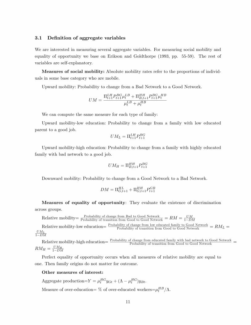
3.1 De�nition of aggregate variables

We are interested in measuring several aggregate variables. For measuring social mobility and

equality of opportunity we base on Erikson and Goldthorpe (1993, pp. 55-59). The rest of

variables are self-explanatory.

Measures of social mobility: Absolute mobility rates refer to the proportions of individ-uals in some base category who are mobile.

Upward mobility: Probability to change from a Bad Network to a Good Network.

UM =�LHt+1P

BGt+1�

LBt +�HHB;t+1P

BGt+1�

HBt

�LBt + �HBt

We can compute the same measure for each type of family:

Upward mobility-low education: Probability to change from a family with low educated

parent to a good job.

UML = �LHt+1P

BGt+1

Upward mobility-high education: Probability to change from a family with highly educated

family with bad network to a good job.

UMH = �HHB;t+1P

BGt+1

Downward mobility: Probability to change from a Good Network to a Bad Network.

DM = �HLG;t+1 +�HHG;t+1P

GBt+1

Measures of equality of opportunity: They evaluate the existence of discriminationacross groups.

Relative mobility= Probability of change from Bad to Good NetworkProbability of transition from Good to Good Network = RM = UM

1�DM

Relative mobility-low education= Probability of change from low educated family to Good NetworkProbability of transition from Good to Good Network = RML =

UML1�DM

Relative mobility-high education= Probability of change from educated family with bad network to Good NetworkProbability of transition from Good to Good Network =

RMH =UMH1�DM

Perfect equality of opportunity occurs when all measures of relative mobility are equal to

one. Then family origins do not matter for outcome.

Other measures of interest:

Aggregate production=Y = �HGt yGt + (�� �HGt )yBt.

Measure of over-education= % of over-educated workers=�HBt =�:

11

Measure of aggregate human capital= % of people with high education=(�HBt + �HGt )=�:

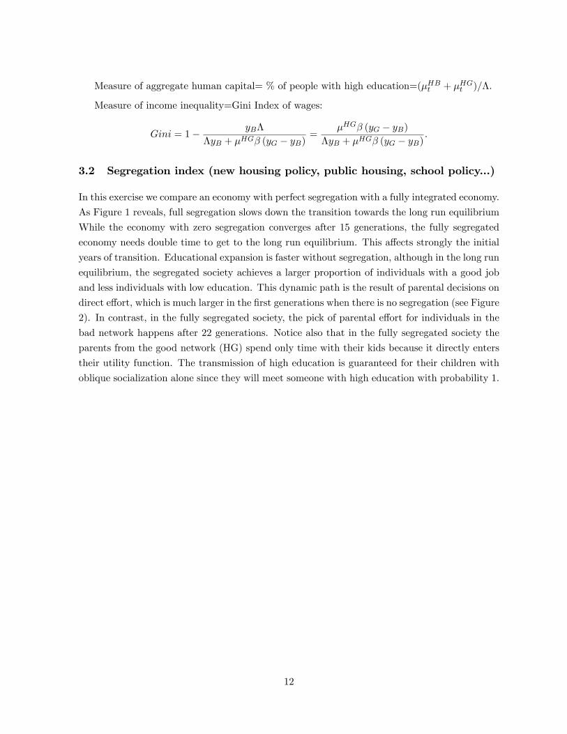
Measure of income inequality=Gini Index of wages:

Gini = 1� yB�

�yB + �HG� (yG � yB)=

�HG� (yG � yB)�yB + �HG� (yG � yB)

:

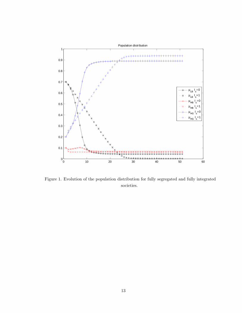
3.2 Segregation index (new housing policy, public housing, school policy...)

In this exercise we compare an economy with perfect segregation with a fully integrated economy.

As Figure 1 reveals, full segregation slows down the transition towards the long run equilibrium

While the economy with zero segregation converges after 15 generations, the fully segregated

economy needs double time to get to the long run equilibrium. This a¤ects strongly the initial

years of transition. Educational expansion is faster without segregation, although in the long run

equilibrium, the segregated society achieves a larger proportion of individuals with a good job

and less individuals with low education. This dynamic path is the result of parental decisions on

direct e¤ort, which is much larger in the �rst generations when there is no segregation (see Figure

2). In contrast, in the fully segregated society, the pick of parental e¤ort for individuals in the

bad network happens after 22 generations. Notice also that in the fully segregated society the

parents from the good network (HG) spend only time with their kids because it directly enters

their utility function. The transmission of high education is guaranteed for their children with

oblique socialization alone since they will meet someone with high education with probability 1.

12

0 10 20 30 40 50 600

0.1

0.2

0.3

0.4

0.5

0.6

0.7

0.8

0.9

1Population distribution

µLB  Is=0

µLB  Is=1

µHB  Is=0

µHB  Is=1

µHG  Is=0

µHG  Is=1

Figure 1. Evolution of the population distribution for fully segregated and fully integrated

societies.

13

0 5 10 15 20 25 30 35 40 45 500.1

0.2

0.3

0.4

0.5

0.6

0.7

0.8

0.9

1Direct parental effort

dLB, Is=0

dLB, Is=1

dHB, Is=0

dHB, Is=1

dHG , Is=0

dHG , Is=1

Figure 2. Parental time devoted to children in fully segregated and fully integrated societies.

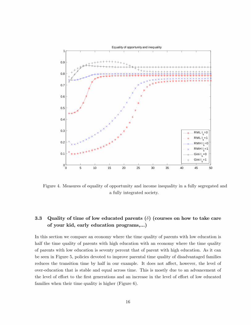
Figures 3 and 4 show the measures of social mobility, equality of opportunity and inequality

for these two economies. Regarding social mobility (Figure 3), the long run equilibrium level of

social mobility is similar for both economies (around 70% of individuals born in a bad network

will end up in the good network). However, the transition paths are very di¤erent. The society

with zero segregation presents a steep increase in social mobility in the �rst ten generations,

while for the fully segregated economy, social mobility changes marginally over the same period

of time. Equality of opportunity is also much higher in the fully integrated society, with faster

convergence to the long run equilibrium (Figure 4). Di¤erences in equality of opportunity are,

however, small in the long run.

The Gini index comes up very large for both economies and while it is larger for the segregated

economy during the �rst 23 generations, the situation reverses afterwards (Figure 4).

14

0 5 10 15 20 25 30 35 40 45 500

0.1

0.2

0.3

0.4

0.5

0.6

0.7

0.8Social mobility

UM Is=0

UM Is=1

UML Is=0

UML Is=1

UMH Is=0

UMH Is=1

Figure 3. Probability of upward mobility for a fully integrated and a fully segregated society.

15

0 5 10 15 20 25 30 35 40 45 500

0.1

0.2

0.3

0.4

0.5

0.6

0.7

0.8

0.9

1Equality of opportunity and inequality

RML Is=0

RML Is=1

RMH Is=0

RMH Is=1

Gini Is=0

Gini Is=1

Figure 4. Measures of equality of opportunity and income inequality in a fully segregated and

a fully integrated society.

3.3 Quality of time of low educated parents (�) (courses on how to take careof your kid, early education programs,...)

In this section we compare an economy where the time quality of parents with low education is

half the time quality of parents with high education with an economy where the time quality

of parents with low education is seventy percent that of parent with high education. As it can

be seen in Figure 5, policies devoted to improve parental time quality of disadvantaged families

reduces the transition time by half in our example. It does not a¤ect, however, the level of

over-education that is stable and equal across time. This is mostly due to an advancement of

the level of e¤ort to the �rst generations and an increase in the level of e¤ort of low educated

families when their time quality is higher (Figure 6).

16

d

0 10 20 30 40 50 600

0.1

0.2

0.3

0.4

0.5

0.6

0.7

0.8

0.9

1Population distribution

µLB δ=0.5

µLB δ=0.7

µHB δ=0.5

µHB δ=0.7

µHG δ=0.5

µHG δ=0.7

Figure 5. Evolution of population distribution for societies with di¤erent quality of time of low

educated parents.

17

0 5 10 15 20 25 30 35 40 45 500.2

0.3

0.4

0.5

0.6

0.7

0.8

0.9

1Direct parental effort

dLB, δ=0.5

dLB, δ=0.7

dHB , δ=0.5

dHB , δ=0.7

dHG , δ=0.5

dHG , δ=0.7

Figure 6. Parental time devoded to children for two societies with di¤erent time quality of low

educated parents.

Obviously, the levels of social mobility and equality of opportunity are larger in the society

where time parental quality is larger (Figures 7 and 8). This keeps true even in the long run

for those individuals with low educated parents. Surprisingly, though, the level of inequality is

signi�cantly larger for the �rst 10 generations in the society with larger time parental quality.

This is due to the rapid increase of individuals in good jobs in this society during this period.

18

0 5 10 15 20 25 30 35 40 45 500.1

0.2

0.3

0.4

0.5

0.6

0.7

0.8Social mobility

UM δ=0.5UM δ=0.7UML δ=0.5UML δ=0.7UMH δ=0.5UMH δ=0.7

Figure 7. Probability of upward mobility for two societies with di¤erent time quality of low

educated parents.

19

0 5 10 15 20 25 30 35 40 45 500.1

0.2

0.3

0.4

0.5

0.6

0.7

0.8

0.9Equality of opportunity and inequality

RML δ=0.5RML δ=0.7RMH δ=0.5RMH δ=0.7Gini δ=0.5Gini δ=0.7

Figure 8. Measures of equality of opportunity and income inequality in two societies with

di¤erent time quality of low educated parents.

3.4 s/S: e¢ ciency units of search for each network.

Here we analyze an economy where probability of �nding a good job if you come from a bad

network is 70% that of someone from a good network and compare it to an economy where this

probability is 90% that of someone from a good network. It turns out that convergence to the

long run equilibrium is faster in the latter economy (Figure 9). Moreover, the level of over-

education is lower when the probability to �nd a job is less dependent on the type of network

you are in. This is due to the fact that a higher s translates into more e¢ ciency units of search,

and therefore, more vacancies are open. Consequently, the number of matches in the good job

sector is larger the larger is s.

20

0 10 20 30 40 50 600

0.1

0.2

0.3

0.4

0.5

0.6

0.7

0.8

0.9

1Population distribution

µLB  s=0.7

µLB  s=0.9

µHB  s=0.7

µHB  s=0.9

µHG  s=0.7

µHG  s=0.9

Figure 9. Evolution of the population distribution for two societies with di¤erent networking

in�uence in the labor market.

In Figure 10 we can see that the long run direct e¤ort of individuals in a bad job does not

depend on the network e¤ects in the labor market. Notwithstanding, during transition, direct

e¤ort of these individuals is increased when s = 0:9, since the expected value of their kid having

high education is larger because the probability of getting a good job increased. Individuals

in the good network seem to decrease their e¤ort from the seventh generation on, suggesting a

substitution e¤ect of their e¤ort by the oblique socialization that occurs more often in a more

educated society.

21

0 5 10 15 20 25 30 35 40 45 500.2

0.3

0.4

0.5

0.6

0.7

0.8

0.9

1Direct parental effort

dLB, s=0.7dLB, s=0.9dHB , s=0.7dHB , s=0.9dHG , s=0.7dHG , s=0.9

Figure 10. Parental time devoted to children in two societies that di¤er in their networking

importance in the labor market.

Upward mobility increases strongly when the e¢ ciency units of search associated to individ-

uals from a bad network increase since it rises aggregate e¢ ciency units of search, enhancing

the creation of new vacancies and creating a larger amount of good jobs. As a consequence,

it is more likely for anyone to change from a bad network to the good network (Figure 11).

Moreover, since changing from s = 0:7 to s = 0:9 we are reducing the di¤erences across types of

family, the equality of opportunity increases signi�cantly (Figure 12).

22

0 5 10 15 20 25 30 35 40 45 500.1

0.2

0.3

0.4

0.5

0.6

0.7

0.8Social mobility

UM s=0.7UM s=0.9UML s=0.7UML s=0.9UMH s=0.7UMH s=0.9

Figure 11. Probability of upward mobility for two societies with di¤erent networking in�uence

in the labor market.

23

0 5 10 15 20 25 30 35 40 45 500.1

0.2

0.3

0.4

0.5

0.6

0.7

0.8

0.9

1Equality of opportunity and inequality

RML s=0.7RML s=0.9RMH s=0.7RMH s=0.9Gini s=0.7Gini s=0.9

Figure 12. Measures of equality of opportunity and income inequality in two societies with

di¤erent impact of networks in the labor market.

3.5 Cost of creating a vacancy: � (reduction of bureaucracy).

Figure 13 shows the evolution of the population distribution in two economies that di¤er in

the cost of creating a vacancy for a good job. An increase in vacancy costs clearly rises the

amount of over-educated individuals in the economy, via a reduction in the amount of vacancies

open. While the transition period length is similar in both cases, changes in the population

distribution are more intense in the �rst generations for the economy with lower vacancy costs.

24

0 10 20 30 40 50 600

0.1

0.2

0.3

0.4

0.5

0.6

0.7

0.8

0.9

1Population distribution

µLB κ=0.5

µLB κ=1

µHB κ=0.5

µHB κ=1

µHG κ=0.5

µHG κ=1

Figure 13. Evolution of population distribution for two societies with di¤erent vacancy costs.

25

0 5 10 15 20 25 30 35 40 45 500.2

0.3

0.4

0.5

0.6

0.7

0.8

0.9

1Direct parental effort

dLB, κ=0.5

dLB, κ=1

dHB , κ=0.5

dHB , κ=1

dHG , κ=0.5

dHG , κ=1

Figure 14. Parental time devoted to children in two societies with di¤erent vacancy costs.

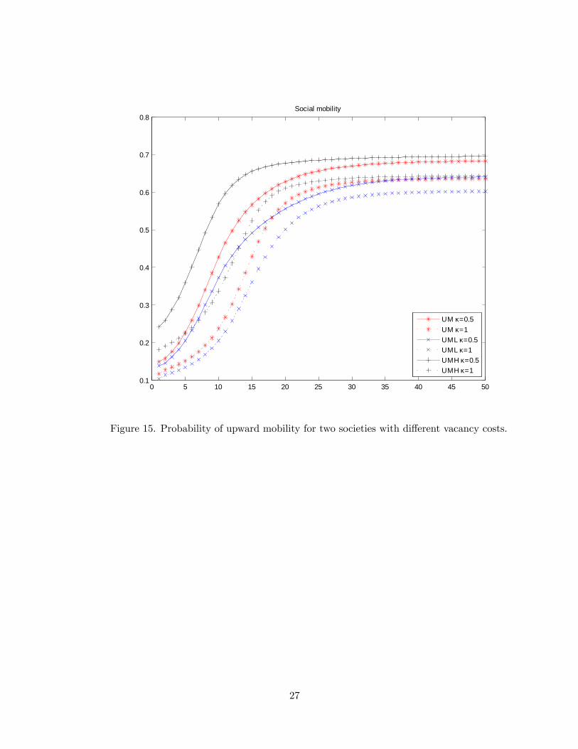
While social mobility is higher in the case of low vacancy costs during transition and in the

long run (Figure 15), equality of opportunity is only signi�cantly larger in the �rst 15 generations

and inequality (Gini index) is also larger (Figure 16).

26

0 5 10 15 20 25 30 35 40 45 500.1

0.2

0.3

0.4

0.5

0.6

0.7

0.8Social mobility

UM κ=0.5UM κ=1UML κ=0.5UML κ=1UMH κ=0.5UMH κ=1

Figure 15. Probability of upward mobility for two societies with di¤erent vacancy costs.

27

0 5 10 15 20 25 30 35 40 45 500.2

0.3

0.4

0.5

0.6

0.7

0.8

0.9

1Equality of opportunity and inequality

RML κ=0.5RML κ=1RMH κ=0.5RMH κ=1Gini κ=0.5Gini κ=1

Figure 16. Measures of equality of opportunity and income inequality in two societies with

di¤erent vacancy costs.

3.6 Worker bargaining power � (presence of unions for instance).

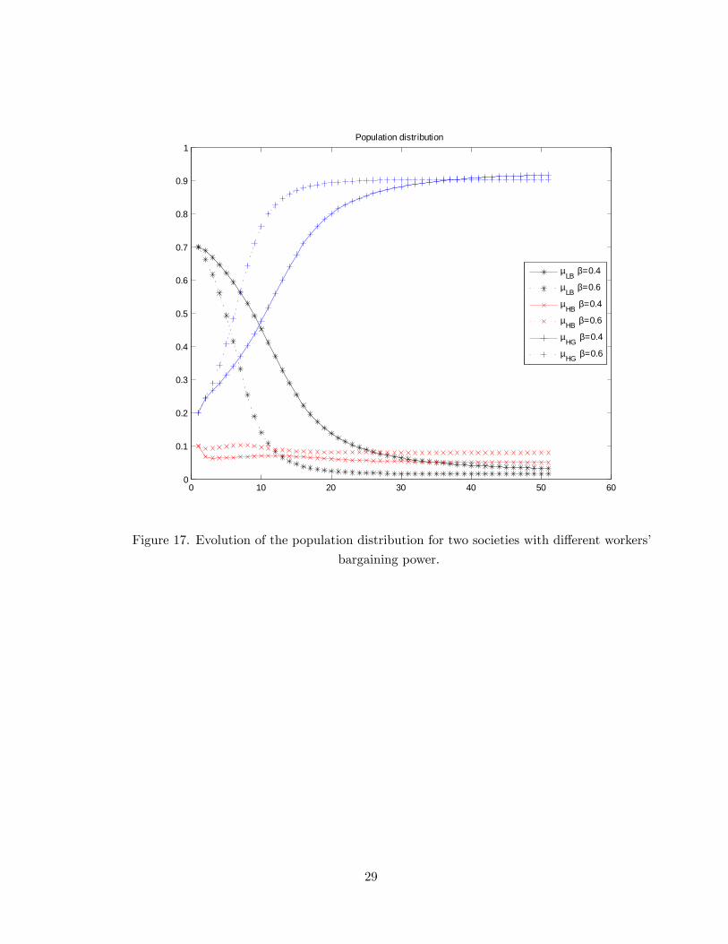
An increase in workers�bargaining power in the economy results in a similar transition period as

with the case of a reduction in vacancy costs, except that over-education now increases (Figure

17). Moreover, in the long run equilibrium, the number of good jobs is lower, since �rms have

less incentives to open vacancies. Similarly as in the previous case, the parental e¤ort increases

for the �rst generations, and specially for the over-educated individuals (Figure 18). This leads

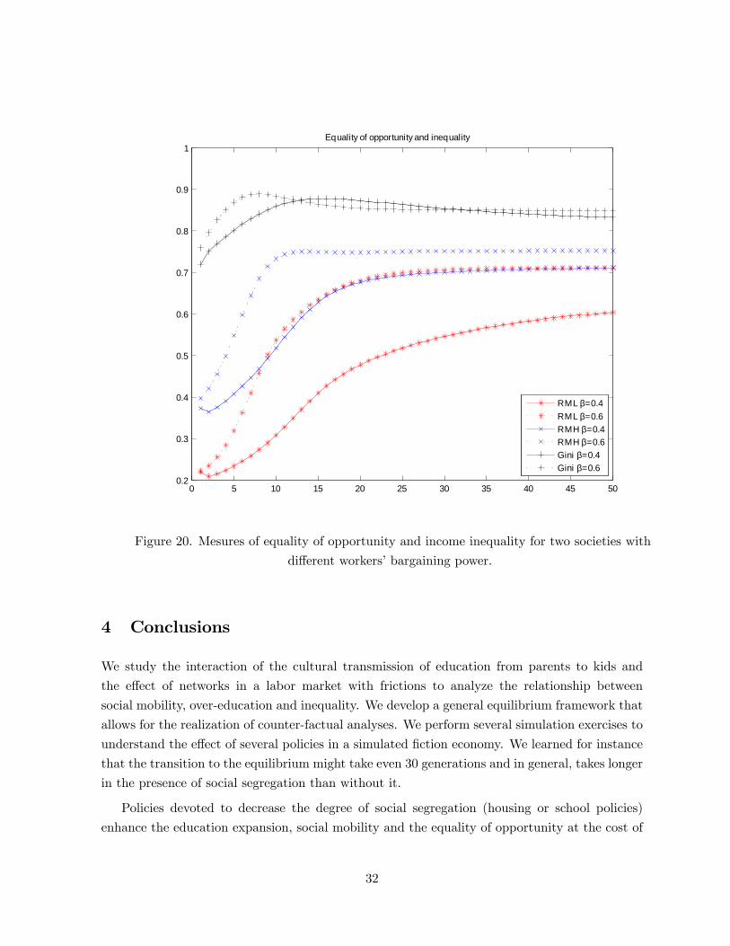
to higher social mobility and a drastic increase in equality of opportunity, with small changes

in inequality mostly for the �rst 10 generations (Figure 20).

28

0 10 20 30 40 50 600

0.1

0.2

0.3

0.4

0.5

0.6

0.7

0.8

0.9

1Population distribution

µLB β=0.4

µLB β=0.6

µHB β=0.4

µHB β=0.6

µHG β=0.4

µHG β=0.6

Figure 17. Evolution of the population distribution for two societies with di¤erent workers�

bargaining power.

29

0 5 10 15 20 25 30 35 40 45 500.2

0.3

0.4

0.5

0.6

0.7

0.8

0.9

1Direct parental effort

dLB, β=0.4

dLB, β=0.6

dHB , β=0.4

dHB , β=0.6

dHG , β=0.4

dHG , β=0.6

Figure 18. Parental time devoted to children in two societies with di¤erent workers�bargaining

power.

30

0 5 10 15 20 25 30 35 40 45 500.1

0.2

0.3

0.4

0.5

0.6

0.7

0.8Social mobility

UM β=0.4UM β=0.6UML β=0.4UML β=0.6UMH β=0.4UMH β=0.6

Figure 19. Probability of upward mobility for two societies with di¤erent workers�bargaining

power.

31

0 5 10 15 20 25 30 35 40 45 500.2

0.3

0.4

0.5

0.6

0.7

0.8

0.9

1Equality of opportunity and inequality

RML β=0.4RML β=0.6RMH β=0.4RMH β=0.6Gini β=0.4Gini β=0.6

Figure 20. Mesures of equality of opportunity and income inequality for two societies with

di¤erent workers�bargaining power.

4 Conclusions

We study the interaction of the cultural transmission of education from parents to kids and

the e¤ect of networks in a labor market with frictions to analyze the relationship between

social mobility, over-education and inequality. We develop a general equilibrium framework that

allows for the realization of counter-factual analyses. We perform several simulation exercises to

understand the e¤ect of several policies in a simulated �ction economy. We learned for instance

that the transition to the equilibrium might take even 30 generations and in general, takes longer

in the presence of social segregation than without it.

Policies devoted to decrease the degree of social segregation (housing or school policies)

enhance the education expansion, social mobility and the equality of opportunity at the cost of

32

a smaller good sector and larger inequality in the long run.

Policies devoted to improve the job matching process (public employment o¢ ces, unemployed

training, reduction of administrative costs to open vacancies) decrease over-education levels

and have a positive impact on social mobility while the e¤ect on equality of opportunity and

inequality is not clear.

Policies that a¤ect the bargaining power of workers have a positive e¤ect on social mobility

and equality of opportunity at the cost of increasing over-education, while leaving inequality

unchanged.

Further work will consist on calibrating the model to real economies in order to verify the

explanatory power of the model. We aim at then using it to assess the e¤ect of alternative

policies on real economies.

References

[1] Becker, G. S. and N. Tomes (1986) "Human capital and the rise and fall of families", Journal

of Labor Economics, Vol. 4, No. 3, pp. 1-39.

[2] Bénabou, R. (2002) "Tax and education policy in a heterogeneous-agent economy: What

levels of redistribution maximize growth and e¢ ciency?", Econometrica, Vol. 70, No. 2, pp.

481-517.

[3] Bentolila, Michelacci and Suarez (2008). "Social Contacts and Occupational Choice",

Economica, Vol. 77, Issue 305, pp. 20-45, January 2010

[4] Bisin, A. and T. Verdier (2001) "The economics of cultural transmission and the evolution

of preferences", Journal of Economic Theory, Vol. 97, No. 2, pp. 298-319.

[5] Björklund, A. and M. Jäntti (2009) "Inter-generational income mobility and the role of fam-

ily background" In Oxford Handbook of Economic Inequality, edited by Wiemer Salverda,

Brian Nolan, and Timothy M. Smeeding, chap. 20. Oxford: Oxford Univ. Press.

[6] Black, S.E. and P.J. Devereux (2011) "Recent developments in inter-generational mobility"

In Handbook of Labor Economics, edited by A. Orley and C. David, Elsevier. Volume 4,

Part B: chap. 16.

[7] Brunello, Garibaldi and Wasmer (2007). "Education and Training in Europe". Oxford Uni-

versity Press, 2007.

[8] Case and Katz (1991) "The Company You Keep: The E¤ects of Family and Neighborhood

on Disadvantaged Youths", NBER Working Paper.

33

[9] Corak, M. and P. Piraino (2011) "The inter-generational transmission of employers", Jour-

nal of Labor Economics, Vol. 29, No. 1, pp. 37-68.

[10] Cutler, D. M. and E. L. Glaeser (1997) "Are ghettos good or bad?", The Quarterly Journal

of Economics, Vol. 112, No. 3, pp. 827-872.

[11] den Haan, W.J, G. Ramey and J. Watson (2000) "Job destruction and propagation of

shocks", The American Economic Review, Vol. 90, no. 3, pp. 482-498.

[12] Erikson and Goldthorpe (1993) "The constant �ux: A Study of Class Mobility in Industrial

Societies", Oxford, Oxford University Press.

[13] Freeman (1976). "The Overeducated American", Academic Press.

[14] Galor, O. and D. Tsiddon (1997) "Technological progress, mobility and growth", American

Economic Review, Vol. 87, pp. 363-382.

[15] Guryan, J., E. Hurst and M. Kearney (2008) "Parental education and parental time with

children", Journal of Economic Perspectives, vol. 22,. no. 3, pp. 23-46.

[16] Hassler, J., S. Rodríguez Mora and J. Zeira (2007) "Inequality and mobility", Journal of

Economic Growth, Vol. 12, No. 3, pp. 235-259.

[17] Heckman, J., R. Pinto and P. Savelyev �Understanding the Mechanisms through Which an

In�uential Early Childhood Program Boosted Adult Outcomes,�. Forthcoming, American

Economic Review.

[18] Ioannides, Y. M. and L. D. Loury (2004) "Job information networks, neighborhood e¤ects,

and inequality", Journal of Economic Literature, Vol. 42, No. 4, pp. 1056-1093.

[19] Kalleberg and Sorensen (1979) �Sociology of Labor Markets.�, Annual Review of Sociology

5:351�79.

[20] Lefgren, L., M. J Lindquist and D. Sims (2012) "Rich dad, smart dad: Decomposing the

inter-generational transmission of income", Journal of Political Economy, Vol. 120, No. 2,

pp. 268-303.

[21] Loury, G. C. (1981) "Inter-generational transfers and the distribution of earnings", Econo-

metrica, Vol. 49, pp. 843-867.

[22] Maoz, Y.D. and O. Moav (1999) "Inter-generational mobility and the process of develop-

ment", The Economic Journal, Vol. 109, No. 458, pp. 677-697.

[23] Mayer, A. (2008) "Education, self-selection, and inter-generational transmission of abili-

ties", Journal of Human Capital, Vol. 2, No. 1, pp. 106-128.

34

[24] O�Regan and Quigley (1996) "Teenage employment and the spatial isolation of minority

and poverty households", Journal of Human Resources, Vol. 31, No.3, pp.692-702.

[25] Patacchini, E. and Y. Zenou (2011) "Neighborhood e¤ects and parental involvement in the

inter-generational transmission of education", Journal of Regional Science, Vol. 51, No. 5,

pp. 987-1013.

[26] Restuccia, D. and C. Urrutia (2004) "Inter-generational persistence of earnings: the role of

early and college education", The American Economic Review, Vol. 94, No. 5, pp. 1354-

1378.

[27] Ribó, A. and M. Vilalta-Bufí (2012) "Is the matching function Cobb-Douglas?", UB Work-

ing Paper.

[28] Sicherman and Galor (1990) "A Theory of Career Mobility," Journal of Political Economy,

University of Chicago Press, vol. 98(1), pages 169-92.

[29] Solon, G. (1999) "Inter-generational mobility in the labor market" In Handbook of Labor

Economics, Vol. 3, edited by Orley Ashenfelter and David Card, pp. 1761-1800. Amsterdam:

Elsevier.

35