Distributed Inference: Combining Variational · Combining Variational ... The study of inference...

Combining Variational

Inference With Distributed Computing

by

Chris Calabrese

S.B. Computer Science and Engineering,Massachusetts Institute of Technology, 2011

Submitted to the

ARC6 W;e F H/E

jj9

Department of Electrical Engineering and Computer Sciencein partial fulfillment of the requirements for the degree of

Master of Engineering in Electrical Engineering and Computer Science

at the

MASSACHUSETTS INSTITUTE OF TECHNOLOGY

February 2013

Massachusetts Institute of Technology 2013. All rights reserved.

A u th o r ..............................................................Chris Calabrese

Department of Electrical Engineering and Computer Science

/IfCertified by

U

February 5, 2013

David WingateResearch ScientistThesis Supervisor

Accepted by........Prof. Dennis M. Freeman

Chairman, Masters of Engineering Thesis Committee

Distributed Inference:

Distributed Inference: Combining Variational Inference

With Distributed Computing

by

Chris Calabrese

Submitted to the Department of Electrical Engineering and Computer Scienceon February 5, 2013, in partial fulfillment of the

requirements for the degree ofMaster of Engineering in Electrical Engineering and Computer Science

Abstract

The study of inference techniques and their use for solving complicated models hastaken off in recent years, but as the models we attempt to solve become more complex,there is a worry that our inference techniques will be unable to produce results.Many problems are difficult to solve using current approaches because it takes toolong for our implementations to converge on useful values. While coming up withmore efficient inference algorithms may be the answer, we believe that an alternativeapproach to solving this complicated problem involves leveraging the computationpower of multiple processors or machines with existing inference algorithms. Thisthesis describes the design and implementation of such a system by combining avariational inference implementation (Variational Message Passing) with a high-leveldistributed framework (Graphlab) and demonstrates that inference is performed fasteron a few large graphical models when using this system.

Thesis Supervisor: David WingateTitle: Research Scientist

3

Acknowledgments

I would like to thank my thesis advisor, David Wingate, for helping me work through

this project and dealing with my problems ranging from complaints about Matlab

to my difficulties working with some of the mathematical concepts in the study of

inference. Most importantly, his efforts helped me develop some kind of intuition for

the subject matter relevant to this project, and that is something I know I can use

and apply in the future.

5

Contents

1 Introduction

1.1 Example: Inference on Seismic Data . . . . . .

1.2 Variational Message Passing and Graphlab . . .

1.2.1 Variational Inference and VMP . . . . .

1.2.2 Distributed Computation and Graphlab

1.3 Contributions . . . . . . . . . . . . . . . . . . .

2 Variational Message Passing

2.1 Bayesian Inference . . . . . . . . . . .

2.1.1 Example: Fair or Unfair Coin? .

2.2 Variational Inference . . . . . . . . . .

2.3 Variational Message Passing . . . . . .

2.3.1 Message Construction . . . . .

2.3.2 Operation Details . . . . . . . .

3 Graphlab Distributed Framework

3.1 Parallel/Distributed Computation . . .

3.1.1 Parallel Computing . . . . . . .

3.1.2 Distributed Computing . . . . .

3.2 Parallel/Distributed Frameworks . . .

3.2.1 Distributed VMP Framework .

3.3 Graphlab Distributed Framework . . .

3.3.1 Graphlab PageRank Example .

7

11

12

14

14

15

16

17

. . . . . . . . . . . . . . . . . 17

. . . . . . . . . . . . . . . . . 18

. . . . . . . . . . . . . . . . . 21

. . . . . . . . . . . . . . . . . 23

. . . . . . . . . . . . . . . . . 24

. . . . . . . . . . . . . . 25

29

. . . . . . . . . . . . . . . . . 29

. . . . . . . . . . . . . . . . . 30

. . . . . . . . . . . . . . . . . 32

.. . . .. . .. . . . . .. . . 34

.. . . .. . . .. . . . .. . . 35

. .. . .. . . . .. . . . .. . 37

.. . . . .. . .. . . . .. . . 4 1

4 VMP/Graphlab Implementation Details 49

4.1 VMP Library ........ ............................... 51

4.1.1 Supported Models ........................ . 57

4.2 VMP/Graphlab Integration ....................... 61

4.2.1 Creating The Factor Graph ...... ................... 62

4.2.2 Creating The Vertex Program . . . . . . . . . . . . . . . . . . 63

4.2.3 Scheduling Vertices For Execution . . . . . . . . . . . . . . . . 65

4.3 Graphical Model Parser . . . . . . . . . . . . . . . . . . . . . . . . . 67

4.4 Current Limitations . . . . . . . . . . . . . . . . . . . . . . . . . . . . 68

5 Results 71

5.1 Parallel Test Results . . . . . ... . . . . . . . . . . . . . . . . . . . 71

5.2 Distributed Test Results . . . .. . . . . . . . . . . . . . . . . . . . . 76

6 Conclusion 81

A Coin Example: Church Code 83

B VMP Message Derivations 85

B.1 Gaussian-Gamma Models . . . . . . . . . . . . . . . . . . . . . . . . 86

B.2 Dirichlet-Categorical Models . . . . . . . . . . . . . . . . . . . . . . . 90

8

List of Figures

1-1 Complicated inference example: Seismic data [11] . . . . . . . . . . . 13

2-1 Results from performing inference on the fairness of a coin. Observed

Data = 3H, 2T; Fairness Prior = 0.999 . . . . . . . . . . . . . . . . . 19


Data = 5H; Fairness Prior = 0.999 . . . . . . . . . . . . . . . . . . . 20







2-6 Variational Inference: High-Level Diagram . . . . . . . . . . . . . . . 21

2-7 VMP Example: Gaussian-Gamma Model . . . . . . . . . . . . . . . . 27

3-1 Typical Parallel Computing Environment [28] . . . . . . . . . . . . . 30

3-2 Typical Distributed Computing Environment [28] . . . . . . . . . . . 33

3-3 Graphlab: Factor Graph Example [33] . . . . . . . . . . . . . . . . . 38

3-4 Graphlab: Consistency Models [33] . . . . . . . . . . . . . . . . . . . 40

3-5 Graphlab: Relationship Between Consistency and Parallelism [33] . . 41

4-1 VMP/Graphlab System Block Diagram . . . . . . . . . . . . . . . . . 49

4-2 Supported Models: Gaussian-Gamma Model . . . . . . . . . . . . . . 57

4-3 Supported Models: Dirichlet-Categorical Model . . . . . . . . . . . . 58

9

4-4 Supported Models: Gaussian Mixture Model [27] . . .

4-5 Supported Models: Categorical Mixture Model [27] . .

Parallel VMP Execution Time: Mixture Components

Parallel VMP Execution Time: Observed Data Nodes

Parallel VMP Execution Time: Iterations . . . . . . . .

Distributed VMP Execution: Real Time . . . . . . . .

Distributed VMP Execution: User Time . . . . . . . .

Distributed VMP Execution: System Time . . . . . . .

B-i VMP Message Derivations: Gaussian-Gamma Model .

B-2 VMP Message Derivations: Dirichlet-Categorical Model

10

5-1

5-2

5-3

5-4

5-5

5-6

58

59

. . . . . 72

. . . . . 74

. . . . . 75

. . . . . 78

. . . . . 79

. . . . . 79

86

90

Chapter 1

Introduction

The ideas associated with probability and statistics are currently helping Artificial

Intelligence researchers solve all kinds of important problems. Many modern ap-

proaches to solving these problems involve techniques grounded in probability and

statistics knowledge. One such technique that focuses on characterizing systems by

describing them as a dependent network of stochastic processes is called probabilistic

inference. This technique allows researchers to determine the hidden quantities of

a system from the observed output of the system and some prior beliefs about the

system behavior.

The use of inference techniques to determine the posterior distributions of variables

in graphical models has allowed researchers to solve increasingly complex problems.

We can model complicated systems as graphical models, and then use inference tech-

niques to determine the hidden values that describe the unknown nodes in the model.

With these values, we can predict what a complicated system will do with different

inputs, allowing us access to a more complete picture describing how these systems

behave.

Some systems, however, require very complex models to accurately represent all

their subtle details, and the complexity of these models often becomes a problem

when attempting to run inference algorithms on them. These intractable problems

can require hours or even days of computation to converge on posterior values, making

it very difficult to obtain any useful information about a system. In some extreme

11

cases, convergence to posterior values on a complicated model may be impossible,

leaving problems related to the model unsolved.

The limitations of our current inference algorithms are clear, but the effort spent

in deriving them should not be ignored. Coming up with new inference algorithms,

while being a perfectly acceptable solution, is difficult and requires a lot of creativity.

An alternative approach that makes use of existing inference algorithms involves

running them with more computational resources in parallel/distributed computing

environments.

Since computational resources have become cheaper to utilize, lots of problems

are being solved by allocating more resources (multiple cores and the combined com-

putational power of multiple machines) to their solutions. Parallel and distributed

computation has become an cheap and effective approach for making problems more

tractable, and we believe that it could also help existing inference techniques solve

complicated problems.

1.1 Example: Inference on Seismic Data

Consider an example problem involving the use of seismic data to determine what

parts of the earth may be connected. This has practical applications relating to effi-

cient drilling for oil, where the posterior distribution describing the layers of sediment

in the earth provides invaluable information to geologists when determining what lo-

cations for drilling are more likely to strike oil and not waste money. Figure 1-1 shows

an example of seismic data.

The seismic data was generated by shooting sound waves into the ground and

waiting for the waves to bounce back to the surface, giving an idea of where each

layer of sediment is located relative to the layers above and below it. From this

information, we want to determine which horizontal sections (called "horizons") are

connected so that geologists have a clearer picture of when each layer of sediment was

deposited. This is a difficult problem because the "horizons" are hardly ever straight

lines and can only be determined by combining global information (for example, the

12

Figure 1-1: Complicated inference example: Seismic data [11]

orientation of horizons on each side of the bumps in the above figure) with local

information (for example, adjacent pixels in a particular horizon).

This example is particularly useful for motivating the complicated inference prob-

lem because it is difficult to perform inference over the graphical models used to

encode all the necessary information of this physical system. The global informa-

tion requires that models representing this system have lots of edges between nodes

(resulting in lots of dependencies in the inference calculations). The local informa-

tion requires that the model has a very large number of nodes (since each pixel is

important and needs to be accounted for in some way). The result is a complicated

graphical model that our current inference techniques will have trouble describing in

a reasonable amount of time.

With parallel/distributed computation, there may be ways to perform inference on

different parts of the graphical model at the same time on different cores or machines,

saving all the time wasted to perform the same computations in some serial order. It

is clear that inference problems will not usually be embarrassingly parallel (that is,

easily transformed into bunch of independent computations happening at the same

time), but there is certainly a fair amount of parallelism to exploit in these graphical

models that could increase the tractability of these complicated problems.

13

1.2 Variational Message Passing and Graphlab

The difficulty in coming up with a parallel/distributed inference algorithm comes

from finding the right set of existing tools to combine, and then finding the right way

to combine them such that the benefits of parallel/distributed computing are real-

ized. This thesis will describe the design process in more detail later, but the solution

we eventually decided on was a combination of a variational inference implementa-

tion, called Variational Message Passing [32], and a relatively high-level distributed

computation framework based on factor graph structures, called Graphlab [33].

1.2.1 Variational Inference and VMP

Variational inference [19, 26] refers to a family of Bayesian inference techniques for

determining analytical approximations of posterior distributions for unobserved nodes

in a graphical model. In less complicated terms, this technique allows one to approx-

imate a complicated distribution as a simpler one where the probability integrals can

actually be computed. The simpler distribution is very similar to the complicated

distribution (determined by a metric known as KL divergence [15]), so the results of

inference are reasonable approximations to the original distribution.

To further provide a high-level picture of variational inference, one can contrast it

with sampling methods of performing inference. A popular class of sampling methods

are Markov Chain Monte Carlo methods [7, 2, 21], and instead of directly obtaining

an approximate analytical posterior distribution, those techniques focus on obtaining

approximate samples from a complicated posterior. The approximate sampling tech-

niques involve tractable computations, so one can quickly take approximate samples

and use the results to construct the posterior distribution.

The choice to use variational inference as the target for combination with par-

allel/distributed computing is due to a particular implementation of the algorithm

derived by John Winn called Variational Message Passing (VMP) [32]. The VMP

algorithm involves nodes in a graphical model sending updated values about their

own posterior distribution to surrounding nodes so that these nodes can update their

14

posterior; it is an iterative algorithm that converges to approximate posterior values

at each node after a number of steps. The values sent in the update messages are

derived from the mathematics behind variational inference.

The emphasis on iterative progression, graphical structure, and message passing

make this algorithm an excellent candidate for integrating with parallel/distributed

computation. These ideas mesh well with the notion of executing a program on

multiple cores or multiple machines at once because the ideas are also central to the

development of more general parallel/distributed algorithms.

1.2.2 Distributed Computation and Graphlab

With a solid algorithm for performing variational inference, we needed to decide

on some approach for adding parallelism and distributed computing to everything.

The primary concerns when choosing a parallel/distributed framework were finding

a good balance between low-level flexibility and high-level convenience, and finding a

computation model that could mesh well with the VMP algorithm. After looking at

a few options, we eventually settled on the Graphlab [33] framework for distributed

computation.

Graphlab is a distributed computation framework where problems are represented

as factor graphs (not to be confused with graphical models in Bayesian inference). The

nodes in the factor graph represent sources of computation, and the edges represent

dependencies between the nodes performing computation. As computation proceeds,

each node in the graph updates itself by gathering data from adjacent nodes, applying

some sort of update to itself based on the gathered data, and then scattering the new

information out to the adjacent nodes. Any nodes that are not connected by edges can

do this in parallel on multiple cores, or in a distributed fashion on multiple machines.

The Graphlab framework has a number of qualities that meshed very well with

our constraints. For one, the library provides a useful high-level abstraction through

factor graphs, but achieves flexibility through the fact that lots of problems can be

represented in this way. Once a problem has been represented as a factor graph, the

Graphlab internal code does most of the dirty work relating to parallel/distributed

15

computation. Another useful quality is the ease in switching from parallel compu-

tation on multiple cores to distributed computation on multiple machines; this only

requires using a different header file and taking a few special concerns into account.

Finally, the particular abstraction of a factor graph appears to be compatible with

the emphasis on graphical structure inherent to the VMP algorithm, and we believed

this would make combining the two ideas much easier.

1.3 Contributions

Apart from the ideas in this paper, this thesis has produced two useful pieces of soft-

ware that can be used and extended to help solve problems in the field of probabilistic

inference.

1. A functional and modular VMP library has been implemented in C++ that

currently has support for a number of common exponential family distributions.

The feature set of this implementation is not as deep as implementations in other

languages, such as VIBES [32, 13] in Java or Infer.NET [20] in C-Sharp, but it

can be extended easily to add support for more distribution types in the future.

2. An implementation combining the Graphlab framework and the VMP library

described above has also been created. The combined Graphlab/VMP code has

the same functionality as the original VMP library, and performs inference for

some larger graphical models faster than the unmodified code does.

The remainder of this thesis is organized as follows: Chapters 2 and 3 provide

a detailed look at the components of our implementation by describing the design

considerations and component parts of the Variational Message Passing library and

the Graphlab distributed framework. Chapter 4 describes the implementation details

of the combined Variational Message Passing / Graphlab code that we have produced.

Chapter 5 demonstrates some results that show the correctness and increased speed

of the system we have created. Chapter 6 concludes this paper and discusses some

other relevant work for this topic.

16

Chapter 2

Variational Message Passing

This chapter will describe the Variational Message Passing (VMP) [32] algorithm in

greater detail. The VMP algorithm, as summarized in the introduction, is an imple-

mentation of variational inference that uses a factor graph and message passing to

iteratively update the parameters of the posterior distributions of nodes in a graphi-

cal model. The ideas of general Bayesian inference, and more specifically, variational

inference will be reviewed before describing how the VMP algorithm works.

2.1 Bayesian Inference

The VMP algorithm is a clever implementation of variational inference, which refers

to a specific class of inference techniques that works by approximating an analytical

posterior distribution for the latent variables in a graphical model. Variational in-

ference and all of its alternatives (such as the Markov Chain Monte Carlo sampling

methods mentioned in the introduction) are examples of Bayesian inference. The

basic ideas surrounding Bayesian inference will be reviewed in this section.

Bayesian inference refers to techniques of inference that use Bayes' formula to

update posterior distributions based on observed evidence. As a review, Bayes' rule

says the following:

P(HID) = P(DIH).P(H) (2.1)P(D)

17

The components of equation 2.1 can be summarized as:

1. P(HID): The posterior probability of some hypothesis (something we are test-

ing) given some observed data.

2. P(DIH): The likelihood that the evidence is reasonable given the hypothesis in

question.

3. P(H): The prior probability that the hypothesis in question is something rea-

sonable.

4. P(D): The marginal likelihood of the observed data; this term is not as im-

portant when comparing multiple hypotheses, since it is the same in every

calculation.

Intuitively, the components of Bayes' formula highlight some of the important

points about Bayesian inference. For one, it becomes clear that the posterior dis-

tribution is determined as more observed data is considered. The components also

imply that both the hypothesis and the considered evidence should be reasonable.

For the evidence, this is determined by the likelihood factor, and for the hypothesis,

this is determined by the prior. The prior probability factor is very important, since

it sways the posterior distribution before having seen any observed evidence.

2.1.1 Example: Fair or Unfair Coin?

The following example is adapted from the MIT-Church wiki [9]. Church is a high-

level probabilistic programming language that combines MIT-Scheme [8] with prob-

abilistic primitives such as coin flips and probability distributions in the form of

functions. This thesis will not describe probabilistic programming in any detail, but

for more information, one can look at the references regarding this topic [5, 31, 30].

For the purposes of this example, Church was used to easily construct the relevant

model and produce output consistent with the intuition the example attempts to de-

velop. The code used to generate the example model and the relevant output can be

found in Appendix A.1.

18

Consider a simple example of a probabilistic process that should make some of

the intuitive points about Bayesian inference a little clearer: flipping a coin. At the

start of the simulation, you don't know anything about the coin. After observing the

outcome of a number of flips, the task is to answer a simple question: "is the coin fair

or unfair?" A fair coin should produce either heads or tails with equal probability

(weight = 0.5), and an unfair coin should exhibit some bias towards either heads or

tails (weight 5 0.5).

Say you observe five flips of the coin, and note the following outcome: 3 heads

and 2 tails. When prompted about the fairness of the coin, since there is really no

evidence to support any bias in the coin, most people would respond that the coin

is fair. Constructing this model in Church and observing the output backs this fact

up, as demonstrated by the histogram in Figure 2-1. The histograms produced by

Church in this section will count "#t" and "#f" values, corresponding to "true" (the

coin is fair) and "false" (the coin is unfair). As you can see, all 1000 samples from

the posterior distribution report that the coin is believed to be fair.

Fair Coin (3H, 2T)?

0 200 400 600 800 1000 1200

Figure 2-1: Results from performing inference on the fairness of a coin. ObservedData = 3H, 2T; Fairness Prior = 0.999

What happens when the outcome changes to 5 consecutive heads? Believe it or

not, most people would probably still believe the coin is fair, since they have a strong

prior bias towards believing that most coins are fair. Observing five heads in a row is a

little weird, but the presented evidence isn't really enough to outweigh the strength of

the prior. Histograms for five heads with a strong prior bias towards fairness (Figure

2-2) and with no bias at all (Figure 2-3) are provided below.

19

Fair Coin (5H, Fairness Prior = 0.5)?

0 200 400 600 800 1000

sames

1200 0 200 400 600 800

sample

Figure 2-2: Results from performinginference on the fairness of a coin. Ob-served Data = 5H; Fairness Prior =

0.999


0.500

As you can see, both the prior and the evidence are important in determining the

posterior distribution over the fairness of the coin. Assuming we keep the expected

prior in humans that has a bias towards fair coins, it would take more than five heads

in a row to convince someone that the coin is unfair. Figure 2-4 shows that ten heads

are almost convincing enough, but not in every case; Figure 2-5 shows that fifteen

heads demonstrate enough evidence to outweigh a strong prior bias.

Fair Coin (0OH, Fairness Prior = 0.999)?

0 100 200 300 400 500 600 700

Figure 2-4: Results from performinginference on the fairness of a coin. Ob-served Data = 1OH; Fairness Prior =

0.999

Fair Coin (1 5H, Fairness Prior = 0.999)?

at.

200 400 600 300 1000


0.999

If someone is generally more skeptical of coins, or if they have some reason to

believe the coin flipper is holding a trick coin, their fairness prior would be lower,

and the number of consecutive heads to convince them the coin is actually unfair

20

~1

1000 1200

Fair Coin (5H, Fairness Prior =0.999)?

would be smaller. The essence of Bayesian inference is that both prior beliefs and

observed evidence affect the posterior distributions over unknown variables in our

models. As the above example should demonstrate, conclusions about the fairness of

the coin were strongly dependent on both prior beliefs (notions about fair coins and

the existence of a trick coin) and the observed evidence (the sequence of heads and

tails observed from flipping the coin).

2.2 Variational Inference

The actual process by which one can infer posterior distributions over variables from

prior beliefs and observed data is based on derivations of probability expressions

and complicated integrals. One such technique that focuses on approximating those

posterior distributions as simpler ones for the purposes of making the computations

tractable is called variational inference. Variational inference techniques will result

in exact, analytical solutions of approximate posterior distributions. A high-level,

intuitive picture of how variational inference works is provided in Figure 2-6:

Class of distributions P(Z)

Actual posterior: P(Z I X)Tractable approximations of P(Z): Qo(Z)

Target posterior: tractable Qe(Z) closest to actual P(Z I X)with m ( dist ( Qe(Z) 11 P(Z I X)))

Figure 2-6: Variational Inference: High-Level Diagram

21

The large outer cloud contains all posterior distributions that could explain the

unknown variables in a model, but some of these distributions may be intractable.

The distributions inside the inner cloud are also part of this family, but the integrals

used for calculating them are tractable. The variable 0 parameterizes the family of

distributions Q(Z) such that Qo(Z) is tractable.

The best Qo(Z) is determined by solving an optimization problem where we want

to minimize some objective function over 0 based on the actual posterior and the

family of tractable distributions. The minimum value of the objective function cor-

responds to the best possible QO(Z) that approximates the actual posterior P(ZIX).

The best approximate posterior distribution will describe the unknown variable about

as well as the actual posterior would have.

The objective function that is generally used in variational inference is known as

KL divergence. Other divergence functions can be used, but the KL divergence tends

to provide the best metric for determining the best approximation to the actual

posterior distribution. The expression for KL divergence is in terms of the target

approximate posterior Q and the actual posterior P is given below1 .

DKL(QIIP) = Q(Z) log P(X) (2.2)

The optimization problem of minimizing the KL divergence between two probabil-

ity distributions is normally intractable because the search space over 6 is non-convex.

To make the optimization problem easier, it is useful to assume that Qo will factor-

ize into some subset of the unknown variables. This is the equivalent of removing

conditional dependencies between those unknown variables and treating the posterior

distribution as a product of the posterior distributions. The factorized expression for

Qo becomes:

M

Qo(Z) = l q(Zi jX) (2.3)i=1

'The LaTeX code for the equations in this section come from http://en.wikipedia.org/wiki/VariationalBayesianmethods

22

The analytical solution for Qo(Z) then comes from the approximate distributions

qj to the original factors q3. By using methods from the "calculus of variations," one

can show that the approximate factor distributions with minimized KL divergence

can be expressed as the following:

eEisa [in p(Z,X)]

q)(Z3 X) = f eEisAlInP(z,x)l dZ(

In qj*(Zj IX) = Eig[lnp(Z, X)] + constant (2.5)

The Eigj [lnp(Z, X)] term is the expectation of the joint probability between the

unknown variables and the observed evidence, over all variables not included in the

factorized subset.

The intuition behind this expression is that it can usually be expressed in terms of

some combination of prior distributions and expectations of other unknown variables

in the model. This suggests an iterative coordinate descent algorithm that updates

each node in some order, using the updated values of other nodes to refine the value

computed at the current node.

This idea essentially describes how variational inference is generally implemented:

initialize the expectations of each unknown variable based on their priors, and then

iteratively update each unknown variable based on the updated expectations of other

variables until the expectations converge. Once the algorithm converges, each un-

known variable has an approximate posterior distribution describing it.

2.3 Variational Message Passing

The Variational Message Passing (VMP) algorithm follows the same intuition de-

scribed at the end of the previous section: it is an algorithm that iteratively updates

the posterior distributions of nodes in a graphical model based on messages received

from neighboring nodes at each step.

The details specific to the implementation of this particular implementation of

23

variational inference surround the use of messages. The nodes in a graphical model

interact (send and receive messages) with other nodes in their Markov blankets; that

is, their parents, children, and coparents. The messages contain information about

the current belief of the posterior distribution describing the current node. As the

beliefs change with information received from other nodes, the constructed messages

sent out to other nodes will also change. Eventually, the values generated at each

node will converge, resulting in consistent posterior distributions over every node in

the model.

2.3.1 Message Construction

Constructing the messages sent between a particular pair of nodes is relatively dif-

ficult, but by restricting the class of models to "conjugate-exponential" models, the

mathematics behind the messages can be worked out. The two requirements for these

models are:

1. The nodes in the graphical model must be described by probability distribu-

tions from the exponential family. This has two advantages: the logarithms

involved in computation are tractable, and the state of these distributions can

be summarized entirely by their natural parameter vector.

2. The nodes are conjugate with respect to their parent nodes; in other words, the

posterior distribution P(XIY) needs to be in the same family of distributions as

the prior distribution P(Y) (where Y is a parent of X in the graphical model).

This has one advantage: iterative updating of the posterior distributions of

nodes only changes the values and not the functional form of the distribution.

Once these requirements are enforced, the source of the messages can be directly

observed from the exponential family form expression:

P(XIY) = exp[q(Y)'u(X) + f (X) + g(Y)] (2.6)

24

In particular, the messages sent from parents to children (Y -+ X) are some

function of the natural parameter vector /(Y), and the messages sent from children

to parents (X -+ Y) are some function of the natural statistic vector u(X). The other

functions in the above expression are for normalization purposes and do not affect

the content of the constructed messages.

The natural parameter vector is determined by expressing a distribution in the

exponential family form described above, and taking the part of the expression that

depends on the parent nodes. The natural statistic vector is determined by taking

the expectation of the vector containing the moments of a distribution. The pro-

cess for obtaining each vector is different depending on the model in question, but

once the vectors are determined, they can be directly inserted into the algorithm

implementation for constructing messages.

For derivations of the natural parameter vectors and messages used in the models

that the combined VMP/Graphlab implementation can support, see Appendix B for

more information.

2.3.2 Operation Details

Determining the content of messages is work that needs to be done before the al-

gorithm is actually run on a graphical model. Once the message content is coded

into the algorithm, the actual operation of the algorithm follows a specific process

that ensures each node in the graphical model ends up with the correct approximate

posterior distribution. The steps performed at each node in the VMP algorithm are:

1. Receive messages from all of your parents. These messages will be used in

updating your natural parameter vector during the update step.

2. Instruct your coparents to send messages to their children. This ensures that the

children will have the most current information about the posterior distributions

of nodes in your Markov blanket when they send you messages in the next step.

3. Receive messages from all of your children. These messages will be summed up

and used to update your natural parameter vector during the update step.

25

4. Update your natural parameter vector by combining information about your

prior with the messages you received from your parents and children. Once

the natural parameter vector is current, use it to update your natural statistic

vector for future messages you send to any children you have.

The above steps are performed once at each node during a single step of the

algorithm. Once all nodes have been updated, the algorithm starts again with the

first node. The algorithm terminates either after a set number of steps, or when the

natural parameter vector at each node converges to some consistent value.

The update step for a particular node involves updating the natural parameter

vector for that distribution. The derivations of natural parameter vectors for specific

models supported by the combined VMP/Graphlab code are part of the work detailed

in Appendix B. In general, the update step for a given node involves summing all the

messages received from your children, and then adding that sum to the initial values

of your natural parameter vector.

The following example demonstrates how the mu node in a Gaussian-Gamma

model is updated during the first step of the VMP algorithm. The graphical model

in question is provided in Figure 2-7. The circles with labels are the nodes in the

graphical model; the leaf nodes with d, labels are the observed data nodes, and

everything else is an unknown variable. The uncircled numbers at the top of the

model are the hyperparameters that define the prior distributions over the top-level

nodes. The Gaussian and Gamma distributions are part of the exponential family,

and the Gaussian-Gamma parent pair for Gaussian-distributed observed data satisfies

the conjugacy constraint, so VMP can be performed on this model.

The steps taken for updating the mu node during the first iteration of the VMP

algorithm are:

1. The mu node does not have any parents, so do not receive any messages.

2. The children of mu all have prec as a parent, so prec is a coparent of mu and

must send messages to the d, child nodes.

26

(mu, ss

Gaussmean

(shape, rate) prior

1.0 1.0

shape prior

) prior 0.0 1.0 1.0 rate Ga!par

ian Gammaparent mu prec precision

dO da d2 d3

Gaussian distributed observed data

mnma rateent

parent

Figure 2-7: VMP Example: Gaussian-Gamma Model

3. The d child nodes have been updated, so mu should receive current messages

from all of them.

4. The mu node now has all the information about the believed posterior distri-

bution of every node in its Markov blanket, so it can combine everything and

update its own natural parameter vector and natural statistic vector.

The same steps would apply to prec during the first iteration (with the added

note that prec will receive messages from rate in the first step), and the algorithm

will keep updating mu and prec during each iteration until the natural parameter

vector at both nodes converges to consistent values. The nodes should be visited in

topological order during each iteration of the algorithm; in the above example, this

means the effective order is {rate, mu, prec}.

As a final note, the observed data nodes already have defined values (we are

not determining posterior distributions for observed evidence), so only the unknown

variables need to explicitly have an update step. The observed data in the leaf

nodes becomes important when the unknown variables directly above them receive

messages from the observed nodes; these messages contain the observed data as part

27

of the message and their upward propagation ensures that the unknown variables in

the model take the observed evidence into account.

28

Chapter 3

Graphlab Distributed Framework

This chapter will describe the Graphlab [33] framework in more detail. The Graphlab

framework takes problems represented as factor graphs and executes them on multi-

ple cores or machines. The vertices of the factor graph represent individual parts of

the problem, and the edges connecting them represent computational dependencies

between those parts. The abstraction provided by Graphlab strikes an important bal-

ance between flexibility and difficulty in the implementation of parallel/distributed

VMP code. This chapter will review some of the basic concepts surrounding paral-

lel/distributed computing, and then focus on the design and implementation of the

Graphlab framework.

3.1 Parallel/Distributed Computation

The study of parallel/distributed computation involves trying to find ways to leverage

multiple processors or multiple machines to solve problems. The "parallel" aspect of

computation comes from the processors operating in parallel to solve problems, and

the "distributed" aspect of computation comes from multiple computers communi-

cating on some kind of network to solve a problem together.

There is usually no straightforward way to convert a parallel program to a dis-

tributed one, but as the section on Graphlab will explain later, the Graphlab frame-

work abstracts that difference away, allowing programs written with the framework

29

to be easily deployed on a cluster of machines. While this makes implementing your

program easier, it is still important to have some idea of how each deploy method is

different.

3.1.1 Parallel Computing

A typical parallel computing environment will involve multiple processors and some

sort of shared memory that each one will use for reading/writing data. Figure 3-

1 demonstrates such a system; the arrows represent the read/write pathways, and

the boxes represent components of the machine (either one of the processors, or the

shared memory).

|Processor Processor Processor

Memory j

Figure 3-1: Typical Parallel Computing Environment [28]

The above image doesn't describe some of the concerns that must be addressed

when writing parallel programs. For one, correctness is not guaranteed when simply

moving a program from a serial environment to a parallel one. When a program is

compiled, it becomes a series of instructions designed to run on a particular archi-

tecture. When spreading a sequential stream of instructions over multiple streams

running at the same time, care must be taken to respect the read/write dependencies

between different instructions. Consider the source code example in Listing 3.1:

#include <stdio.h>

void transfer(int *pl, int *p2, int amount) {*pl = *pl - amount;*p2 = *p2 + amount;

}

void main(int argc , char **argv) {int *pl = malloc(sizeof(int));

30

int *p2 = malloc(sizeof(int));*pl = 100;*p2 = 100;

transfer(pl, p2, 50);transfer(pl, p2, 25);

print f(" pl: f/d\n" ,*pl );print f ("p2: 'od\n" ,*p 2 );

}Listing 3.1: Parallel Dependencies: Transfer Code

When run in a serial environment, the output of the code should be p1 = 25

and p2 = 175. The two pointers have been initialized to hold a total of 200, and

that total is preserved when the transfer requests are run in series. If the code

above were run in parallel such that each transfer request was executed on a different

processor, the results could be different. The lines of code in the transfer function

compile down to several assembly instructions each, so there is a high possibility of

interleaving instructions. In general, when writing parallel programs, any interleaving

of instructions should be assumed possible without locks or other forms of protection.

One such interleaving that could cause major problems is when the LD(*pl) in-

struction in the second transfer request occurs before the ST(*pl) instruction at the

end of the first transfer. In other words, the second transfer request may use the old

value for *p1 and incorrectly subtract 25 from 100, instead of subtracting 25 from 50.

The end result would be p1 = 75 and p2 = 175, which is obviously not what should

happen after executing two transfers. There are several other ways to interleave the

instructions that could produce incorrect results, so special care must be taken when

writing parallel programs.

There are many ways to ensure that shared memory is manipulated in the right

order within parallel programs; the most common way involves the use of locks. A

lock around some data prevents other processors from reading/writing it until the

lock is released. Other examples of concurrency protection will not be discussed here,

but can be explored in the references [23, 18, 12].

In the above example, each transfer call would lock *p1 and *p2 before modifying

31

them, and then release the lock when they are finished. This ensures that the two

transfer requests cannot interleave and produce incorrect results. Listing 3.2 shows

how locking manifests itself in the above example (of course, the specific implemen-

tation depends on the language/framework being used):

#include <stdio .h>

void transfer(int *pl, int *p2, int amount) {77 Lock p1 and p2 before modifying their values so any

7/ other processors will block until they are released

lock(pl); lock(p2);

*pl = *pl - amount;*p2 = *p2 + amount;

/7 Release p1 and p2 so any processors waiting at the

7/ lock calls above can continue

release(p2); release(pl);

}Listing 3.2: Parallel Dependencies: Transfer Code With Locking

A closer look at what actually happens shows that the program instructions are

actually just run in some serial order. This leads into another concern with parallel

programming: efficiency. In the absence of data dependencies, running several parts

of a complicated program concurrently should make the program run faster. While

parallel programs have some overhead in starting up and combining the results of

each processor at the end, that time is easily offset by the amount saved by executing

each part of the program at the same time. When dependencies force serialization of

the instructions to occur, the overhead becomes an additional cost that might not be

worth it.

3.1.2 Distributed Computing

All of the problems described in the parallel computing section are concerns when

writing programs to run on multiple machines. The added level of complexity in writ-

ing distributed programs comes from the addition of some communication network

32

required so that each machine can send messages to each other. Figure 3-2 demon-

strates what a typical distributed environment would look like with the same labels

for processors and memory used in the parallel computing diagram:

Pmcessor

Memo

~Processo

memory

PProcessor

Memory

Figure 3-2: Typical Distributed Computing Environment [28]

Each of the problems described above (correctness and efficiency) are amplified

when working with distributed clusters of machines because the additional require-

ment of communication between each machine is difficult to coordinate correctly.

Imagine if each of the transfer operations in Listing 3.1 were being run on different

machines: there would be significant latency between when one machine updates *p1

and *p2, and when the other machine becomes aware of this update. The lack of

actual shared memory between the two machines introduces new problems to the

system.

The problem of correctness becomes more difficult to solve because locking mech-

anisms will also require communication on the network. A typical solution to dis-

tributed locking involves adding another machine to the network whose only purpose

is to keep track of which machines hold locks for various data shared over the network.

This adds significant complexity to most applications, especially when each machine

on the network is performing local operations in parallel with those distributed locks.

33

The code in Listing 3.2 may still be applicable in a distributed system, but the un-

derlying locking mechanism would be significantly more complicated.

The problem of efficiency becomes even more important to consider because the

overhead cost now includes a significant amount of time devoted to network trans-

mission and message processing. In general, communication networks are assumed to

be unreliable, and measures must be taken at each machine in a distributed cluster to

ensure every message is received in some enforced order. These measures require extra

computation time, and may even delay certain operations from completing. Synchro-

nization between multiple machines in a distributed program is another source of

computation, and in many cases, this could completely kill any gains realized from

an otherwise efficient distributed protocol.

Added to the problems mentioned above is the concern for reliability and fault-

tolerance within distributed programs. In a distributed cluster of computers con-

nected by a network, both machine and network failures are much more common

than individual processor failures in a parallel environment. Accounting for these

failures is difficult and requires even more overhead in most systems. While reliabil-

ity and fault-tolerance will not be described in any more detail with regards to the

VMP/Graphlab system, some useful references can be followed that describe compo-

nents of the replicated state machine method for solving this problem [17, 3].

3.2 Parallel/Distributed Frameworks

With all the problems described in the last section, it should come as no surprise

that most programs using parallel/distributed environments use pre-existing libraries

and frameworks for implementing their code. These libraries and frameworks handle

many of the complicated details associated with solving the problems outlined above

while providing a high-level abstraction for writing parallel/distributed programs.

In the case of parallel programming, most pre-existing support comes in the form of

programming language primitives. In a lower-level language like C, primitive libraries

such as pthreads [4] can be used; this library exposes threads and mutexes, but requires

34

that the programmer explicitly use these constructs to control parallel operation at a

fine-grained level. In a higher-level language like Java, the explicit use of locks is not

always required, since the language abstracts them away by implementing thread-safe

keywords for synchronization [22].

In the case of distributed programming, support within a programming language

is not as common, so programs usually incorporate separate systems to handle the

details of distributed computing. These systems provide their own abstractions that

make the task of dealing with distributed machines way more manageable.

One such example is the Remote Procedure Call (RPC) framework [1], where

programs on individual machines make function calls that actually execute on other

machines and have the return value sent across the network to the calling machine.

Another example is System Ivy [14], where the programs on individual machines

access what appears to be shared memory on the distributed network. These ab-

stractions require complicated implementations to ensure correct operation, but once

completed and tested thoroughly, they can be placed under the hood of other dis-

tributed programs and reliably be expected to work.

3.2.1 Distributed VMP Framework

Taking all of the concerns surrounding parallel/distributed computation into account,

we needed to find a framework that would seemingly mesh well with the VMP algo-

rithm. Three specific frameworks were examined in great detail, with the idea that

each one was representative of some class of frameworks:

1. Message Passing Interface (MPI): a low-level framework that provides basic

support for sending messages between computers on a network [29]. This frame-

work provides no high-level abstraction, but provides a high degree of flexibility

since any kind of system can be built around the provided message passing

primitives.

2. MapReduce: a high-level framework that reduces the problem of distributed

computation to simply providing a map and reduce function to execute in a

35

specific way on a cluster of machines [6]. This framework provides an easy

abstraction to work with, but makes it impossible to solve many problems that

cannot be represented in the underlying structure of the system.

3. Graphlab: a mid-level framework that requires representing a distributed prob-

lem as a factor graph filled with computation nodes and edges describing the

data dependencies between those nodes [33]. This framework requires work to

represent a problem in the factor graph format, but handles many of the other

details of distributed computation once the graph is constructed.

In general, the pattern with most distributed frameworks is that flexibility is

usually traded off with complexity. The lower-level frameworks provide simpler prim-

itives that can be molded into many different systems, but at the cost of needing to

write overly complicated code that needs to deal with many of the gritty details of

distributed computation. The higher-level frameworks deal with almost all of those

details in their underlying implementations, but at the cost of restricting the kinds

of problems they can solve to ones that fit nicely in the provided abstraction.

Using MPI would require that the distributed VMP implementation contain extra

infrastructure code for dealing with data dependencies in the variational inference

updates. The actual schedule of passing messages would need to be controlled at

a relatively low level, so that each node can correctly update itself without using

stale data from a previous iteration. This would be difficult, but clearly possible,

since nothing restricts the kinds of systems that can be molded around the message

passing primitives.

Using MapReduce would probably not be possible because the VMP algorithm has

more data dependencies than the underlying structure of MapReduce can support.

The MapReduce framework tends to be useful for problems that can be broken down

into independently running parts that need to be combined after all processing has

occurred. The ease of using MapReduce comes from the restrictive abstraction that

only works effectively for certain kinds of problems, so although this framework would

remove almost all of the distributed computing concerns, it did not seem useful for

36

implementing the VMP algorithm.

The Graphlab framework seemed to find a sweet spot between the flexibility pro-

vided by MPI and the abstraction provided by MapReduce. The abstraction provides

high-level support for distributed computation while actually fitting the problem we

need to solve; the factor graph abstraction is restrictive, but seems to mesh well

with the emphasis on graphical structure inherent to the VMP algorithm. As men-

tioned earlier, the Graphlab framework also provides a way to easily switch between

parallel and distributed execution, making it easier to deploy the code in different

environments. All in all, the Graphlab framework seemed like the correct choice for

implementing a distributed VMP algorithm with the least difficulty.

3.3 Graphlab Distributed Framework

The Graphlab framework, as mentioned earlier, performs distributed computation on

problems represented as factor graphs. The underlying implementation of Graphlab

handles the concerns described in the parallel/distributed computing section while

enforcing an abstraction that "naturally expresses asynchronous, dynamic, and graph-

parallel computation" [33]. The majority of the effort in using Graphlab to solve a

problem comes from constructing the factor graph to represent a particular problem;

an example of an arbitrary factor graph is provided in Figure 3-3.

The numbered circles are the vertices of the factor graph, and the lines connecting

them are the edges. Both the vertices and the edges can store user-defined data, which

is represented by the gray cylinders in the image (the thin ones with labels Di are

vertex data, and the wide ones with labels Die- are edge data). The scope of each

vertex refers to the data that can be read and/or modified when a vertex is updating

itself during computation. For a given vertex, the scope is defined by the outgoing

edges and the vertices connected by those edges. The overall structure of the graph

cannot be changed during computation, so the vertices and edges are static.

Once the graph is constructed, the framework performs computation on the struc-

ture using a user-defined "vertex program" that uses something called the Gather-

37

Scope s-1

Figure 3-3: Graphlab: Factor Graph Example [33]

Apply-Scatter (GAS) paradigm. The computation model requires that a function be

written for each of these three operations. These functions will be called during each

iteration of the Graphlab computation on each node in the graph. The purpose of

each function is summarized below:

1. Gather: a function that will be called at each vertex once for each of its adjacent

edges. Every pair consisting of a node and one of its adjacent edges will call

this function before any apply operations are started. This function is typically

used to accumulate data from adjacent vertices to be used in an update during

the apply step; when the + and + = operations are defined for the declared

type stored in each node, accumulation happens automatically and the sum is

passed directly to the apply function.

2. Apply: a function that will be called exactly once for each vertex in the graph

with the accumulated sum calculated during the gather step as an argument.

Every vertex will call this function only after all the gather functions have com-

pleted, but before any scatter operations are started. This function is typically

used to update the data stored in a vertex. This is the only function whose

method signature allows for vertex data to be changed; vertex data structures

must be marked as constant in the arguments to gather and scatter.

38

3. Scatter: a function that will be called at each vertex once for each of its adjacent

edges, similar to gather. Every pair consisting of a node and one of its adjacent

edges will call this function only after every apply operation has finished. This

function is typically used to push new data out to the adjacent edges of a vertex

after an update has completed in the apply step. This data will be grabbed by

adjacent vertices during the gather step in the next iteration. Similar to the

apply step, the edge data structures are not marked as constant in the arguments

to this function.

The gather, apply, and scatter functions will execute on each vertex whenever the

vertex is signaled. Normally, after constructing a graph, each node will be explicitly

signaled once to begin executing some algorithm. The GAS functions will execute one

iteration of the algorithm and, unless some convergent value or maximum number of

steps has been reached, each vertex will signal itself to run again for another iteration.

This signaling mechanism must be explicitly included in the vertex program. When

the vertices stop signaling themselves to run, the algorithm ends and the resulting

values can be examined in the nodes.

The exposure of the signaling mechanism is an example of how the Graphlab

abstraction allows some flexibility to solve different kinds of problems. While there is

a standard way for coordinating the signals between nodes so that a typical iterative

algorithm can run, an ambitious problem can use fine-grained control of the signals

to create interesting update schedules.

Another example of this is evident in the consistency models Graphlab exposes for

performing the GAS computations in parallel. While Graphlab handles the compli-

cated details of parallel/distributed programming under the hood, the API provides

higher-level ways to influence how the computation will actually proceed. This has

a direct influence on correctness and efficiency, but it allows the user to find the bal-

ance that works best for a particular program. The consistency models provided by

Graphlab are outlined in Figure 3-4.

The consistency model chosen by the user directly affects the subset of the scope

that a vertex is allowed to read and/or modify during an update step. The full-

39

Read

Figure 3-4: Graphiab: Consistency Models [33]

consistency model allows complete access to the entire scope of a vertex. This disal-

lows the nodes in that scope from executing their own update functions in parallel

with the current vertex, providing the highest amount of consistency. This decreases

the degree to which parallel computation can occur, so lesser consistency models are

provided.

The edge-consistency model is slightly less consistent, only allowing a vertex to

modify the data on its adjacent edges, but read all the data in its scope. The edges

may still not be involved in parallel computation with this model, however, so a

final, lower consistency model is also provided: the vertex-consistency model. The

vertex-consistency model only allows reads and writes to occur on the adjacent edges,

allowing Graphlab the highest amount of freedom to execute node updates in parallel.

In general, consistency and parallelism are traded off differently in each of the

consistency models, and the right one to use depends heavily on the constraints of

the problem being solved. Figure 3-5 summarizes the trade-off for the three models

provided by Graphlab; the highlighted regions represent data that cannot be updated

in parallel in the specified consistency model.

The other low-level details of how Graphlab actually constructs the factor graph on

a distributed cluster of machines and performs computation with multiple machines

40

L

Figure 3-5: Graphlab: Relationship Between Consistency and Parallelism [33]

will not be discussed in significant detail, unless it is relevant to some implementation

detail of the combined VMP/Graphlab system in Chapter 4.

The next part of this section will outline the PageRank [16] example from the

Graphlab tutorial [34] to solidify the intuition behind how the abstraction works and

how it should be used to write distributed programs. For more information on the

implementation details of the Graphlab framework, follow the reference to the VLDB

publication [33].

3.3.1 Graphlab PageRank Example

The PageRank algorithm assigns a numerical weighting to each node in an graph

that is based on how "important" the node is relative to the others in the graph.

This weighting is determined from some function involving the importance of nodes

pointing to the current node and a damping factor included to represent a small ran-

dom assignment of importance. For the purposes of this example, the psuedocode

provided in the Graphlab tutorial (adapted to look like a standard C program in List-

ing 3.3) provides a perfect starting point for implementing this code in the Graphlab

framework:

#include <stdio.h>

41

void main(int argo , char **argv) {// Iterate through all the nodes in the graph

for (int i = 0; i < graph. size(); i++) {Node node = graph->getNode (i );

7/ Compute the pagerank of this node based on77 the pagerank of nodes connected on in-edgesdouble acc = 0;for (int j = 0; j < node.countInEdges(); j++) {

Node inNode = node. getInNode(j);ace = ace + (inNode.pagerank / inNode.countOutEdges());

}

/7 Update the pagerank of this nodenode.pagerank = (0.85 * ace) + 0.15;

}

Listing 3.3: Example PageRank Psuedocode

The final goal is to implement this algorithm using a Graphlab factor graph and

the GAS paradigm so that the PageRank algorithm can easily run on multiple cores

or multiple machines. The process for writing a Graphlab program for the PageRank

algorithm involves two major steps: creating the factor graph and writing the vertex

program to perform the PageRank updates.

The creation of the factor graph is a relatively simple process due to the widespread

use of templates throughout the Graphlab library. The Graphlab primitives are avail-

able to use once a particular header file is included. Once the primitives are available,

creating the factor graph involves defining structures for the vertex and edge data,

and registering them with a specific instance of a graph. Listing 3.4 demonstrates

how this looks:

#include <string>#include <graphlab.hpp>

// Define the vertex data structurestruct vertex-data {

7/ Store the name and pagerank of a node/7 inside each vertex

42

std :: string pagename;double pagerank;

// Constructors for creating vertex..data structsvertex-data(:pagerank(O.0) { }explicit vertex-data(std :: string name): pagename (name),

pagerank (0.){ }

/7 Serialization methods to send and receive7/ vertex-data structs over the networkvoid save (graphlab:: oarchive& oarc) const {

oarc << pagename << pagerank;

}void load(graphlab::iarchive& iarc) {

iarc >> pagename >> pagerank;

}

7/ Type definition of the factor graph based on7/ the vertex-data defined above and an empty type7/ (since edge-data is not needed)typedef graphlab:: distributed -graph<

vertex.data , graphlab ::empty> graph-type;

7/ Initialization stuff that needs to happen7/ to commit the graphint main(int argc , char** argv) {

graphlab ::mpi-tools :: init (argc, argv);graphlab:: distributed control dc;graphlab :: mpi-tools :: finalize (;

}Listing 3.4: PageRank Factor Graph Creation Code

Once the factor graph is created, loading it with data is also relatively easy.

Graphlab provides functions for adding vertices with a specific ID, and then connect-

ing two vertex IDs with through a function that adds edges. Listing 3.5 demonstrates

the general idea behind using these functions:

#include <string>#include <graphlab. hpp>

// Initialization stuff that needs to happen

43

// to commit the graphint main(int argc , char** argv) {

graphlab:: mpi-tools :: init (argc, argv);graphlab:: distributed-control dc;

77 Actually define a graph using the graph-type

/7 template defined earlier

graph-type graph(dc);

/7 Create three vertices using the add..vertex

77 method; note that the ID type is simply

/7 another use of templatinggraphlab:: vertex-id.type vid;for (int i = 0; i < 3; i++) {

vid = i;graph. add-vertex (vid , vertex.data ("node" + i));

}

7/ Add edges between certain nodes using/7 the add-edge method and the vertex IDs

7/ created abovegraph.add-edge(0, 1);graph.add-edge(1, 2);graph.add-edge(2, 0);

graphlab:: mpi-tools :: finalize (;

}Listing 3.5: PageRank Factor Graph Loading Code

The final part of the Graphlab PageRank program involves writing a vertex pro-

gram that implements the PageRank updates in the GAS paradigm, and continues

to schedule itself until the algorithm converges on consistent values. This is best

explained by demonstrating commented code as with the last two parts; Listing 3.6

demonstrates what it looks like:

#include <string>#include <graphlab.hpp>

// Create the vertex programclass pagerank.program :

// Define the template type for the vertex program:

44

/7 the first type is the graph-type , and the second77 type is the type of data stored in each nodepublic graphlab :: ivertex.program<graph-type , double>,

// Required syntax for defining the programpublic graphlab ::ISPOD-TYPE {

private:

/7 Create a local variable to assist in dynamic/7 signaling of verticesbool perform-scatter;

public:

7/ Create the gather operation: note that it/7 will receive a vertex and one of its adjacent/7 edges when invokeddouble gather (icontext -type& context,

const vertex-type& vertex,edge-type& edge) const {

/7 Code performing some part of the PageRank/7 calculations to be accumulated in the apply stepreturn edge.source ().data(.pagerank /

edge. source (). num-outedges (;

}

/7 Create the apply operation: note that the total/7 variable will store the accumulated sums for the/7 vertex in question from the gather stepvoid apply(icontext-type& context,

vertex-type& vertex,const gather-type& total) {

/7 Code updating the pagerank based on the data/7 collected from other nodes in the gather stepdouble newval = total * 0.85 + 0.15;double prevval = vertex. data. pagerank;vertex. data(). pagerank = newval;

/7 Check whether the pagerank has converged, and/7 store this check in the local variableperform-scatter = (std:: fabs(prevval - newval) > 1E-3);

}

45

77 Function that determines what edges the scatter

77 operation will affect: leverage this to implement

// dynamic signalingedge-dir-type scatter-edges (icontext-type& context

const vertex.type& vertex) const {

7/ If the pagerank did not converge in the apply step,

/7 specify that we want scatter to occur on all the

/7 outgoing edgesif (perform-scatter) return graphlab::OUTEDGES;

/7 Otherwise, specify that scattering should occur on

7/ none of the adjacent edges

else return graphlab::NOEDGES;

}

7/ Create the scatter operation: note that it will receive

7/ a vertex and one of its adjacent edges when invoked

void scatter(icontext-type& context ,const vertex-type& vertex,edge-type& edge) const {

/7 If this function is called with an edge , it means that

7/ the pagerank did not converge (and the perform..scatter

77 variable was set to true), so signal the node on this

/7 outgoing edge to run again

context . signal (edge. target ());}

Listing 3.6: PageRank Vertex Program Code

Once the three vertices we defined in Listing 3.5 are initially signaled, the vertex

program takes over and performs PageRank updates until the values in each node

converge. The Graphlab framework is executing these vertex programs in parallel

(or, with minor changes to the code and environment, on a distributed cluster) with

minimal stress from the programmer.

The C++ syntax used to write the code in this subsection may be difficult to

understand for those not familiar with the language, but the point of demonstrat-

ing code snippets is to give a clear picture of how writing distributed programs with

46

Graphlab should feel. The comments provide a high-level picture of what each impor-

tant line of code is doing, and the entire thing should provide a general idea of what

Graphlab programs usually look like. The PageRank code should also look similar to

some of the code provided in Chapter 4 demonstrating how VMP code is combined

with Graphlab, further building up an intuition for how Graphlab programs work

with the reader.

47

Chapter 4

VMP/Graphlab Implementation

Details

This chapter will describe the design and implementation of the combined VMP/-

Graphlab system in detail. Once all the design considerations from the previous

chapters were taken into account, we designed a modular system that could take a

graphical model as input and output posterior distributions over the unknown vari-

ables in that model. A high-level block diagram of the system is provided in Figure

4-1. Each block in the diagram represents a major component of the system, and the

relative vertical positions of each block represent the layer where that component is

located in the system.

Graphical Models andData

VMPScheduler M

Graphlab Library

I I IDistributed Machines

Figure 4-1: VMP/Graphlab System Block Diagram

49

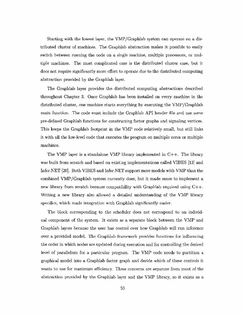
Starting with the lowest layer, the VMP/Graphlab system can operate on a dis-

tributed cluster of machines. The Graphlab abstraction makes it possible to easily

switch between running the code on a single machine, multiple processors, or mul-

tiple machines. The most complicated case is the distributed cluster case, but it

does not require significantly more effort to operate due to the distributed computing

abstraction provided by the Graphlab layer.

The Graphlab layer provides the distributed computing abstractions described

throughout Chapter 3. Once Graphlab has been installed on every machine in the

distributed cluster, one machine starts everything by executing the VMP/Graphlab

main function. The code must include the Graphlab API header file and use some

pre-defined Graphlab functions for constructing factor graphs and signaling vertices.

This keeps the Graphlab footprint in the VMP code relatively small, but still links

it with all the low-level code that executes the program on multiple cores or multiple

machines.

The VMP layer is a standalone VMP library implemented in C++. The library

was built from scratch and based on existing implementations called VIBES [13] and

Infer.NET [20]. Both VIBES and Infer.NET support more models with VMP than the

combined VMP/Graphlab system currently does, but it made sense to implement a

new library from scratch because compatibility with Graphlab required using C++.

Writing a new library also allowed a detailed understanding of the VMP library

specifics, which made integration with Graphlab significantly easier.

The block corresponding to the scheduler does not correspond to an individ-

ual component of the system. It exists as a separate block between the VMP and

Graphlab layers because the user has control over how Graphlab will run inference

over a provided model. The Graphlab framework provides functions for influencing

the order in which nodes are updated during execution and for controlling the desired

level of parallelism for a particular program. The VMP code needs to partition a

graphical model into a Graphlab factor graph and decide which of these controls it

wants to use for maximum efficiency. These concerns are separate from most of the

abstraction provided by the Graphlab layer and the VMP library, so it exists as a

50

separate entity in the system diagram.

The graphical models and data layer contains the format for representing models

that the VMP/Graphlab code can support. Currently, the accepted format and parser

are relatively simple, but emphasis on this layer as a modular component of the system

means that a more complicated language for describing models can replace the simpler

code without compromising the rest of the system. The model and data files can be

manually written or generated with scripts, and the output can be easily accessed

when inference has completed.

The rest of this chapter will explore the finer details about the major components

of the system outlined above. The Graphlab abstraction was described in Chapter 3,

so everything above that layer will be covered in the next few sections.

4.1 VMP Library

The VMP library is a separate component of the system that contains code for per-

forming the VMP algorithm on different graphical models. The library consists of

code describing probability distributions and their behavior during an execution of

the VMP algorithm. Treating the library as a black box, the code takes a graphical

model in some specified text format, and outputs the values characterizing the pos-

terior distributions of any unknown variables in the model. The major components

operating inside the box, in order of control flow, are:

1. parsercpp: This code is responsible for parsing the input graphical model into

some internal structure that the VMP library can use. It reads the specified

text file and creates polymorphic Node objects that contain pointers to all the

information relevant to the VMP algorithm. This is also the location where

checks for conjugate-exponential models can be performed, although the current

version of the code hasn't implemented this yet.

2. node.cpp: This is the pure abstract virtual class that describes nodes in a

graphical model. The classes that inherit from Node share a core set of variables

51

and methods that are the same for any node in a graphical model. When

a particular node requires a specific implementation for some function, that

function is created as virtual in this class and overridden in each specific class

that inherits from Node.

3. *distribution *node. cpp: These are the classes that implement specific probabil-

ity distributions for the VMP algorithm. The parser directly instantiates these

classes based on the information contained in the model file. Before the VMP

algorithm actually begins, objects of this type have initialized natural statistic

and natural parameter vectors; correct parent, children, and coparent lists; and

flags determining whether the node is observed data or not. The message and

update equations for specific distributions are coded directly into methods of

these classes.

4. vmp.cpp: This contains the function that ties together all the other parts of the

VMP library. The input file is passed into this function, and the inference output

is available to it once the VMP algorithm has terminated. The parent, children,

and coparent lists are populated after the parser is invoked, and all necessary

information about the graphical model is compiled and prepared before the

VMP algorithm is actually started. Due to the high degree of modularity in the

system, this is the only file that required a major overhaul when the code was

integrated with Graphlab.

The decision to implement distribution nodes as polymorphic added a fair amount

of effort to the early coding stages, but it has made the code easy to extend in the long

run. Adding new distribution types is simple because most of the relevant information

for nodes is immediately available by inheriting from the pure virtual abstract Node

class. The following source code listing demonstrates exactly which fields are shared

for Node objects:

// Lots of include statements

class Node {

52

protected:

// String identifier for this nodestring name;

77 Vector containing the names of all parents77 to this node in the modelvector<string> parameters;

7/ Flag storing whether this node is observed7/ data and the actual observed data valuebool is-observed;double observed-data;

7/ Enumeration type identifying this node as7/ one of the specific node types (usually7/ not important because of polymorphism)Type type;

7/ Depth in the graphical model (used for7/ determining topological order and the/7 set of coparents)int depth;

/7 Vectors containing polymorphic pointers to7/ the parents, children , and coparents of7/ this particular nodevector<Node *> parents;vector<Node *> children;vector<Node *> coparents;

7/ Declarations of the natural parameter vector7/ and final posterior value vectorvector<double> npv;vector<double> generated-values;

7/ Declarations of the maps associating the7/ messages received at this node with the7/ parents/children that sent themmap<Node *, vector<double> > p2c-messages;map<Node *, vector<double> > c2p-messages;

}

Listing 4.1: Node Class: Shared Fields

53

Not included above are the getter and setter methods that modify all of those

fields. The polymorphic support provided by C++ allows for these fields and methods

to use the generic Node * pointer type because the code will use the right type at

runtime. This is because the class contains pure virtual methods that require specific

implementations to be written in every subclass. These are the methods that are

unique for each probability distribution; the following source code listing explains

their functions:

77 Rest of Node class here

77 Convert the node to a string representation

virtual string to-string () = 0;

// Output the current beliefs about the posteriorvirtual string show-generated-values () = 0;

// Initialize the natural parameter vector

virtual void init-npv() = 0;

// Initialize the eventual output vector

virtual void init-generated-values () = 0;

// Construct a parent to child message

virtual vector<double> make-p2c-msg() 0;

7/ Construct a child to parent messages based on

7/ the target parent and the coparents

virtual vector<double> make-c2p-msg(Node *,

vector<Node *>) = 0;

7/ Update the posterior based on the messages

7/ received from children and your natural

/7 parameter vector (both stored in the class)

virtual void update-generated-values() = 0;

Listing 4.2: Node Class: Pure Virtual Methods

The specific implementations of each class not only implement these virtual meth-

ods, but also provide other fields and methods to make working with specific distri-

butions easier. For example, Gaussian distributions will always have two parameters

54

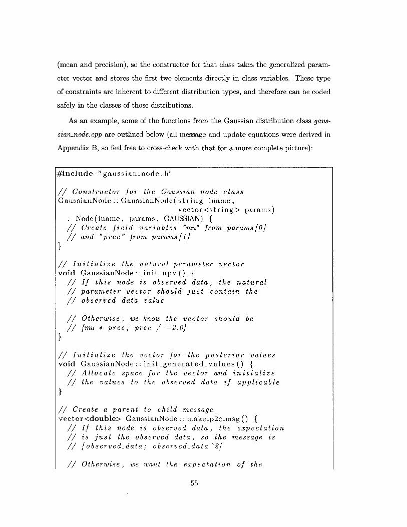
(mean and precision), so the constructor for that class takes the generalized param-

eter vector and stores the first two elements directly in class variables. These type

of constraints are inherent to different distribution types, and therefore can be coded

safely in the classes of those distributions.

As an example, some of the functions from the Gaussian distribution class gaus-

sian-node.cpp are outlined below (all message and update equations were derived in

Appendix B, so feel free to cross-check with that for a more complete picture):

#include "gaussian-node .h"

// Constructor for the Gaussian node classGaussianNode:: GaussianNode( string iname,

vector<string> params)Node (iname, params, GAUSSIAN) {

77 Create field variables "mu" from params[0]7/ and "prec" from params[1]

}

/7 Initialize the natural parameter vectorvoid GaussianNode:: initnpv () {

77 If this node is observed data, the natural7/ parameter vector should just contain the77 observed data value

/7 Otherwise, we know the vector should be

77 [mu * prec; prec / -2.0]

}

/7 Initialize the vector for the posterior valuesvoid GaussianNode:: init -generated-values () {

77 Allocate space for the vector and initialize77 the values to the observed data if applicable

}

77 Create a parent to child message

vector <double> GaussianNode :: make-p2c-msg () {77 If this node is observed data, the expectation77 is just the observed data, so the message is77 [observed-data; observed-data ̂ 2]

77 Otherwise, we want the expectation of the

55

/7 natural statistic vector , which is just7/ [E(X); E(X^2)]

}

7/ Create a child to parent message based on the target

/7 parent and the coparents

vector <double> GaussianNode :: make.c2p-msg (Node * parent,vector<Node *> parents) {

7/ Use the p2c-messages map to obtain the message7/ sent from the coparent and remember it (we will

/7 call it "pmsg")

///7//7

//7//7//7//7

If the target parent has type GAUSSIAN: the messageshould be [E(other) * E(X); E(other) / -2.0], whichis just [pmsg[0] * E(X); pmsg[0] / -2.0]

If the target parent has type GAA&: the

should be [(-0.5 * E(X)^2) - (2.0 * E(X)

+ E(other ̂ 2); 0.5], which is just [(-0.5(2.0 * E(X) * pmsg[0]) + pmsg[1]; 0.5]

message* E(other))* E(X)^2 -

// Update the posterior valuesvoid GaussianNode :: update -generated -values () {

/7 If this node is observed data, do nothing

/7 Otherwise, we need to obtain the natural parameter7/ vector from our parents, which consists of the/7 same quantities as above: [mu * prec; prec / -2.0]

Next, we needfrom childrenand add it to

to sum all the(stored in thethe new NPV we

messages receivedc2p-messages map)obtained above

Finally , we need to obtain the newand prec from the resulting vector;represent the current belief aboutso store them in generated-values

values for muthese values

the posterior,

}

Listing 4.3: Gaussian Node Class: Method Functionality

The VMP library supports a few different kinds of models and implements several

different distribution types. The following subsection outlines those types and goes

56

}

//7//7//7

///7//7//7

into a bit more detail about mixture models that the VMP library supports.

4.1.1 Supported Models

The current VMP library code supports four large classes of conjugate-exponential

models:

1. Gaussian-Gamma Models: This model consists of Gaussian distributed observed

data that has Gaussian parents for the mean parameter and Gamma parents

for the precision parameter. The Gamma nodes can also have Gamma parents

for their rate parameter. As long as a conjugate parent-child pair is Gaussian/-

Gaussian, Gaussian/Gamma or Gamma/Gamma, the system can construct the

right messages and perform inference over the model. An example of this model

is provided below:

(shape, rate) prior

1.0 1.0

(mu, ss

Gausscmean

shape prior

)prior 0.0 1.0 1.0 rate G

ian Gammaparent mu prec precisio

dG d d2 d3


amma ratearent

n parent

Figure 4-2: Supported Models: Gaussian-Gamma Model

2. Dirichlet-Categorical Models: This model consists of Categorically distributed

observed data that has a Dirichlet parent. Dirichlet nodes are not allowed to

have probabilistic parents, so as long as the model consists of Dirichlet/Categor-

57

ical parent-child pairs, the system will produce correct messages and perform

inference over the model. An example of this model is provided below:

psuedocount prior

[1.0, 1.0, 1.0]

dir Dirichlet priorparent

co ci c2 c3

Categorically distributed observed data

Figure 4-3: Supported Models: Dirichlet-Categorical Model

3. Gaussian Mixture Models: This model is similar to the Gaussian-Gamma model

described above, but now K Gaussian/Gamma parent components exist, and

every Gaussian data node is accompanied by a Categorical node that selects

from the different parent components during inference. An example of this

model is provided below:

PO A V 2,02

(Gaussian, Gamma)Prior hyperparameters parent components

[K] K

Dirichlet Categorical Gaussian distributedweights parent selector parent observed data

Figure 4-4: Supported Models: Gaussian Mixture Model [27]

58

4. Categorical Mixture Models: This model is similar to the Dirichlet-Categorical

model, but now K Dirichlet parents exist, and each Categorical data node is

accompanied by another Categorical node that selects from the different parent

components during inference. An example of this model is provided below:

a

Prior hyperparar eters Dirichlet parent6

Dirichlet Categorical Categorically distributedweights parent selector parent observed data

Figure 4-5: Supported Models: Categorical Mixture Model [27]

The messages for the mixture models are based on the particular graphical struc-

ture of each model, a fact that is discussed in another paper discussing Gates [25].

These Gates enclose parts of a graphical model and either turn them on or off based

on the status of the Categorical selector node. This representation makes it possible

to execute the VMP algorithm on mixture models. The message and update equa-

tions were more difficult to derive, so much of the work was double checked against

the values used for mixture code in VIBES.

To implement mixture models, new classes of nodes were made for Gaussian mix-

tures and Categorical mixtures. These nodes are used to represent the observed data

in these models, since when compared to the original Gaussian and Categorical nodes,

they have an extra parent and different messages to send. In particular, these classes

need to send a weighted message to the component parents, and a special kind of

message based on all the components to the selector parent. The following outline

of the child to parent message generating function in the Gaussian mixture class

demonstrates how this works:

59

// Rest of Gaussian mixture node functions here;77 most are very similar to the original Gaussian

77 node class

vector<double> GaussianMixtureNode :: make.c2p-msg(Node *parent , vector<Node *> parents) {

/7 If the target77 the coparents

{//7/7

///7///7

parent is the selector parent, thenconsist of all the component mixtures

Obtain the messages sent by each Gaussian/Gammapair of component parents

Calculate the natural parameter vector from thesemessages [mu * prec; prec / -2.0] and use this vectorto compute a value to insert into the message beingsend to the selector parent

//7///7

Perform the above steps for eachinserting the value for each oneindex in the message

mixture component,into a different

77 Otherwise ,77 components,

{// Obtain the message sent by the selector parent

//7//7//7

77//7//7

Obtain the believed weight that the target mixturecomponent has by taking the right element from theweights message obtained from the selector parent

Multiply the expected message thatto the target parent (based on theby the obtained weight

Listing 4.4: Gaussian Mixture Node: Child To Parent Messages

60

}

the target parent is one of the mixtureand a weighted message should be sent

}

would be senttarget coparents)

4.2 VMP/Graphlab Integration

Once the VMP library described in the previous section was completed, the code

needed to be layered on top of the Graphlab API to allow for parallel/distributed

inference. Due to the modularity of the VMP library and the abstractions provided

by the Graphlab framework, all of the necessary changes were confined to the vmp. cpp

file that drives the VMP code to actually perform inference. The integration effort

required three major steps:

1. Creating the Graphlab factor graph from the VMP graphical model. This re-

quires partitioning the provided graphical model into sets of vertices and con-

necting edges. The VMP/Graphlab code currently imitates the graphical model

structure when constructing the factor graph (each distribution node is treated

as an individual vertex in the factor graph) but this may not be the most effi-

cient way to partition models; this is discussed a little further in the limitations

section at the end of this chapter.

2. Defining the vertex program for performing iterations of the VMP algorithm.

This requires finding a way to translate the control flow in the VMP algorithm

to the Gather-Apply-Scatter paradigm that the Graphlab abstraction enforces.

The VMP library contains most of the code that constructs and passes messages

during the algorithm, but figuring out when to invoke those methods within the

Graphlab vertex program requires some work.

3. Creating an execution engine and schedule the vertices to run. Once the factor

graph and vertex program are created, the driving function in the VMP code

needs to instruct Graphlab how to proceed with execution. The consistency

model needs to be selected, and the vertices in the factor graph need to be

initially signaled. The Graphlab API exposes enough of its internals to allow for

fine-grained control over these things, but simpler settings can also be enabled

to run the program with base settings.

61

4.2.1 Creating The Factor Graph

The creation of the factor graph requires a new data structure to be used in the

vmp.cpp file: a global map associating Node pointers with their Graphlab vertex IDs.

Each Node object created by the parser is eventually added as a vertex to the factor

graph and assigned a vertex ID in the process (which is stored in the map). The

edges are then populated from top to bottom using the children of each node and the

ID map. This process is shown in the following source code listing:

// Assign every single node a vertex-id-typegraphlab:: vertex-id-type vid = 0;map<Node *, graphlab:: vertex-id-type> node-vid;for (it = nodes.begin(; it != nodes.end(); ++it) {

Node *node = it->second;node.vid [node] = vid++;

}

7/ Construct the Graphlab factor graph by creating7/ vectors of nodes and passing them to vertex-datagraph-type graph(dc);for (it = nodes.begin(); it != nodes.end(); ++it) {7/ Create the vector of model nodes; for now, each7/ factor node will contain exactly one model nodeNode *node = it ->second;

// Add the vertex to the graph using the vid mapgraph. add -vertex ( node-vid [node] ,

vertex-data (node->get-name ());

/7 Create edges from each node to all its children;/7 only allow the first distributed process to do this/7 since duplicate edges are not allowedfor (int x = 0; x < node->get-children (). size (); x++) {

if (dc.procid() - 0) {graph. add-edge (nodevid [node],

node-vid [node->get _children ()[x]]);

}}

}Listing 4.5: VMP/Graphlab Integration: Factor Graph Construction

62

4.2.2 Creating The Vertex Program

The creation of the vertex program requires defining gather, apply, and scatter func-

tions for performing the VMP algorithm. The general idea was to handle all the

message passing during the gather step, and handle all the updating during the apply

step, but the delaying of the apply step until all gather operations have completed

made this difficult. Instead, nodes are updated immediately when they have received

all relevant messages in the gather step to produce the same values after inference

as the original VMP library. This results in the apply function only dealing with

signaling vertices for another iteration, and the gather function doing all of the work.

The gather function is executed for all node and adjacent edge pairs in the factor

graph in some parallel/distributed way, so the speed increase in using Graphlab comes

from the ability to perform some of the message construction and update steps in

parallel. The gather function is demonstrated below:

// Define the gather operation for VMPvector<double> gather ( icontext-type &context

const vertex-type &vertex,edge-type &edge) const {

77 Obtain the node pointer corresponding to this name77 by doing a lookup in the global nodes tableNode *node = global-nodes [ vertex . data ().name];Node *other = global-nodes[edge.target ().data().name];

// Make sure the other node on the edge is differentif (node - other) {

other = global-nodes [edge. source (). data ().name];

}

/7 If the other node is the parent of this node, receive77 the downward messageif (is-parent(node, other)) {

vector<double> msg = other ->make-p2c-msg (;node->set _p2c-message (other , msg);

} else if (is-child(node, other)) {77 Otherwise , it is a child node, so all the coparents/7 should send a message upwardsvector<Node *> coparents = other->get-parents (;for (unsigned x = 0; x < coparents . size (; x++) {

63

Node *coparent = coparents [x];if (node != coparent) {

vector<double> msg = coparent->make-p2c-msg (;other ->set _p2c _message (coparent , msg);

}}

7/ After the coparents are done, receive the message

/7 from the childvector <double> msg = other ->make-c2p-msg (node,

other->get _parents ();node->set _c2p-message (other , msg);

}

Order hack: on the first iterationany categorical selector nodes

(context . iteration () 0 &&node->get-type () CATEGORICAL) {

return vector<double>();

Once all the messages are received,values for this node

(node->get-num.p2c-messages ()node->get-parents (). size () &&node->get num-c2p -messages ()node->get -children (). size () {

node->update-generated-values ();

77 The factor graph nodes are

7/ since the VMP library does

/7 vector is returned for thereturn vector<double>();

do not update

update posterior

not storing any values

all the work, so an empty

accumulator to pass along

}

Listing 4.6: VMP/Graphlab Integration: Gather Function

The vertex data only maintains the name of its corresponding graphical model

node because that information is important for obtaining the Node pointers on other

machines that are required arguments to most functions in the VMP library. Most

of the functionality is still coming from the VMP library, but in order to ensure that

the right Node pointers exist on each machine running a gather function, a global

64

///if

}

////i f

}

map associating node names and the memory address in the current memory layout

has been added to vmp.cpp. The first lines of code in each gather function obtain

the correct pointers for the nodes being referenced, and the rest of the function uses

those pointers to call VMP library functions as in the original vmp.cpp functions.

Another problem that Graphlab introduced was executing the gather operation on

each node in an unspecified order due to the nature of running everything in parallel.

This sometimes produces different values than the original VMP library (which used

the topological ordering for nodes in the model) due to different messages being

constructed from different update orders. This is not always a problem, but with

some models, the numbers may be different on certain runs of the VMP algorithm.

4.2.3 Scheduling Vertices For Execution

The scheduler component of the system diagram is a representation of the issues

covered in this subsection. The two main issues that need to be addressed are the

iterative signaling of vertices and the consistency model that Graphlab uses for run-

ning the vertex program. There exist many other controls in the Graphlab API that

can tune how efficient the parallel/distributed execution can be, but these two are the

most important in the current implementation of the system and fairly representative

of the thought process.

The signaling of vertices is initially performed in the same topological order used

by the original VMP library. This doesn't actually enforce an ordering, however,

because some vertices may be located on other machines and the parallel/distributed

execution of each gather function can have different orderings on different runs of the

program.

Each vertex is only explicitly signaled once, and then the vertices signal themselves

until some set number of iterations is reached. The VMP/Graphlab code required

a global counter to keep track of the total number of iterations, and it was used in

the apply function to determine whether a particular vertex should be signaled again.

That mechanism is demonstrated in the following source code:

65

77 Define the apply operation for MP; this function// is primarily used for scheduling vertices in the77 current implementationvoid apply(icontext-type &context

vertex-type &vertex ,const gather-type &total) {

77 Check the current iteration count of this vertex/7 against the global steps counter; if less , signal7/ this vertex to run againif (vertex.data().count < global-steps) {

vertex . data (). count++;context . signal (vertex);

}}

Listing 4.7: VMP/Graphlab Scheduling: Apply Function

Another option for signaling vertices is to explicitly check the posterior values at

each node and determine if they have converged in each apply step. This requires

a bit more effort, but could save a lot of time because variational inference on most

models seems to converge rather quickly (sometimes as quickly as the fifth iteration).

This has nothing to do with the parallel/distributed nature of the code, however, and

is only absent because the original VMP library also used a fixed number of iterations

for performing inference.

As for the consistency model selection, this requires choosing from a "synchronous",

"asynchronous," or "semi-synchronous" engine when creating the object driving the

Graphlab computation. The engine takes the constructed factor graph, a distributed

control object, and a string denoting what kind of engine is desired. The different

settings of the engine are related to the consistency/parallelism trade-off discussed in

Chapter 3.

The "synchronous" setting guarantees that all vertex programs (regardless of

their location on a distributed cluster of machines) will execute serially. The "asyn-

chronous" setting attempts to run vertex programs in parallel, but will exhibit a lower

degree of consistency with the data in the graph. The "semi-synchronous" setting is

a middle ground between the last two options, and attempts to find a better balance

66

between consistency sacrifices and increased parallelism.

Beyond explicitly setting a consistency type, Graphlab does not force the program-

mer to do anything more complicated to construct the computation engine. The API

exposes other lower-level fields and methods for more fine-grained control, but no con-

trols of that sort were used with the VMP/Graphlab computation engine. The VMP

algorithm can be run with any of the three consistency types, and as expected, the

trade-off between consistency and parallelism shows up: lower consistency is slightly

faster, but with a higher amount of incorrect values, and higher consistency is slightly

slower, but the inference reports correct values more often.

4.3 Graphical Model Parser

The parser is a text file parser that expects a particular format for graphical models,

and it reads the file according to this format to construct Node objects. A context-free

grammar describing what the parser expects is provided below:

model -> "graph\n", graph, "data\n", data;

graph -> (name, type, parameters, "\n")+;

type -> "gaussian" I "gamma" I "constant" i

"dirichlet" I "categorical", int I

"mixture:", ("gaussian" I "categorical", int);

parameters -> (number I name), (" ", (number I name))*;

data = (name, number, "\n")+;

name -> string;

string -> ("A-Z I a-z 1 0-9")+;

number -> int I double;

int -> ("O-9")+;

double -> int, ".", int;

67

The name field is what connects entries in the parameter lists to nodes declared

earlier in the input file. The name also connects the data entries to nodes. The

accepted types reflect what the code can currently support; as the number of accepted

models increases, the list of recognized types will grow larger. Also, it is useful to note

that "categorical" types require that the dimensionality of the vector be specified in

the input file (hence, the "int" field showing up next to the type in the grammar).

4.4 Current Limitations

There are several limitations in the current implementation of the VMP/Graphlab

code, and this section will outline a few of them and some thoughts about how to

work around them until a proper fix is introduced.

1. The types of models that the VMP/Graphlab code can support is fairly lim-

ited. While Gaussian and Categorical mixture models can be used for many

different problems, failure to include other distribution types prevents certain

problems that depend on those distributions from being solvable with this code.

The feature set of VIBES includes other distributions, as well as deterministic

(non-probabilistic nodes that tend to represent functions like "sum" and "log-

ical OR"), and it would be excellent if the VMP/Graphlab implementation

eventually boasted a similar feature set.

2. The models that the VMP/Graphlab code support only work in one dimension.

In other words, there is no implicit support for multi-dimensional probability

distributions, like a 3D Gaussian with mean and precision parameters in each

dimension. The VIBES code seems to distinguish between scalar and vector

distributions, and has support for vector distributions that the current VMP/-

Graphlab system does not. This can be worked around, however, if the supplied

models just treat separate dimensions as another node in the graphical model.

This will not work with all models, but it certainly would allow for simpler ones

like the 3D Gaussian referenced above.

68

3. The vertex program written for the VMP/Graphlab code does not make full

use of the GAS paradigm provided by Graphlab. Most of the important com-

putation is bunched in the gather function at the moment because correctness

was the primary concern when developing an initial version of this system. This

version still experiences speedups, but it would be nicer if the VMP steps were

spread out over the GAS operations more smoothly. This could include ideas

like actually using the apply step for updating nodes, or actually using the accu-

mulator working behind the gather operation to sum child to parent messages

and automatically pass the sum to the apply function.

4. The consistency model is somewhat important in determining how often the

VMP/Graphlab code outputs the correct values for inference on a model. The

correct values were determined by running the same models through VIBES

and Infer.NET. The original VMP library always gives the same values for the

models we tested, but the VMP/Graphlab code is sometimes different. This is

related to the lack of control over the ordering of updates and the consistency

model chosen for the computation engine. It would be much better if the set-

tings could be easily exposed to guarantee correctness under a certain set of

constraints, and almost always be correct under another set of constraints that

allows the code to run faster.

5. The distributed computation aspect has a bug that prevents nodes from updat-

ing during each step of the VMP algorithm. The problem appears to be that

Graphlab automatically shards the factor graph over the number of distributed

environments created with "mpiexec" and the nodes in the graphical model do

not receive all of their messages. The update is triggered when all the messages

are received in the gather step, so failure to reach that number of messages

causes many of the nodes to skip their update step. This is a major problem for

correctness, but performance results in distributed environments may still have

some merit because the system is still performing all of the message construction

and passing work as if the updates were going to happen.

69

Chapter 5

Results

This chapter will demonstrate some of the results we obtained from running our com-

bined VMP/Graphlab system on some complicated graphical models. The purpose

of showing these results is to demonstrate that the combined VMP/Graphlab system

performs inference faster than the original VMP library. As mentioned earlier, the

combined VMP/Graphlab has limited functionality, but obtaining increased speeds

with the current functionality shows promise that parallel/distributed inference could

actually be useful for performing inference on complicated models.

The system used for running these tests has eight cores available for use, and

distributed environments were simulated using the mpiexec command to spawn copies

of the VMP executable and execute programs with all of them.

5.1 Parallel Test Results

For the first set of tests, we want to measure how the combined VMP/Graphlab

system responds to different Gaussian mixture models of increasing complexity while

running on a single machine. The mixture model is the most complicated type of

model currently supported by our system, so it provides the best workload for running

these tests.

The Gaussian mixture models we use are generated with a script that reads the

parameters of each component and how much weight each one is given. The script

71

generates a model based on the provided components, and generates observed data

consistent with the entered parameters. This approach allows us to easily check if the

posterior values actually make sense, while quickly generating models with different

characteristics.

The first variable we modify is the number of mixture components in the Gaus-

sian mixture model, while keeping the number of observed data nodes and iterations

constant. The results are visualized as a histogram in Figure 5-1. The total number

of observed nodes is 100 and the total number of iterations is 500. The reported times

are averaged over three independent executions of the code. All times are reported

in seconds.

Inference Time vs. Number of Mixture Components8C

VMP Library 73.2 s70 VMP/Graphlab

60-0

50(50-

E 40-0 31.4s030-

20 - 17.66s

10 -10.,5s

2.97 s 4.53 s10'

3 5 10Number of Mixture Components

Figure 5-1: Parallel VMP Execution Time: Mixture Components

The reported execution times show that VMP/Graphlab converges to the same

values as the original VMP library in significantly faster times. The execution time

ratio appears to be about 7x for the three examples, although it looks like the ratio

decreases slightly as the number of mixture components increases. This could be

related to Graphlab having difficulty matching the same level of parallelism with the

complicated models as it did with the simpler models. This could possibly be remedied

by exerting some lower-level control over the parallel/distributed settings that the

72

Graphlab API exposes, or it could just be an unfortunate property of complicated

models.

The number of mixture components in the model and the reported execution time

seem to be linear with the original VMP library, and the Graphlab times appear to

also follow this pattern. The linear dependence makes sense because adding more

mixture components to a model only requires that extra edges be added between all

the observed data and the new parent components. The Categorical selector nodes

are connected to the observed data, so that part of the graph structure is unaffected

by adding more mixture components. The fact that Graphlab follows a similar linear

pattern is promising because it indicates that the two implementations are probably

performing similar computations. The VMP/Graphlab version performs them in

parallel, so the times are lower, but since they are effectively the same, the linear

pattern remains.

As an added note about parallelism, the time reports for the VMP/Graphlab exe-

cutions consistently reported a "user time" that was about twice as large as the "real

time." The "user time" refers to the amount of time spent performing computation

with processors, and the "real time" refers to the actual wall clock time that has

elapsed.

The graphs throughout this section all depict "real time" because that is the

amount of time one has to wait to view the output of performing inference with the

system. However, it is promising to note that the "user time" is larger than the "real

time" because it implies that multiple processors are performing computations at the

same time. The exact meaning of the fact that it is almost always twice as large

has something to do with how Graphlab generally executes code in parallel; this may

indicate that Graphlab generally decides that running these programs on two cores

is the most efficient thing to do.

The second variable we modify is the number of observed data nodes in the Gaus-

sian mixture model, while keeping the number of mixture components and iterations

constant. The results are visualized as a histogram in Figure 5-2. The total number of

mixture components is 3 and the total number of iterations is 500. The reported times

73

are averaged over three independent executions of the code. All times are reported

in seconds.

Inference Time vs. Number of Observed Data Nodes400

*VMP Library 364.83 s

350 VMP/Graphlab

300-006250-

E 200-P~0

150 --114.07 s

2100 _ 95.67 s

50-1.3 ] [18.03 s20.03 s

0 "' 3.17 s

100 150 200Number of Observed Data Nodes

Figure 5-2: Parallel VMP Execution Time: Observed Data Nodes

The second test case also shows significant speedups when using VMP/Graphlab

over the original VMP library. Many of the same thoughts from the first test case

apply for this example. The relative decrease in execution time ratio is especially

noticeable in this example, as the ratio starts off at about 6x, and ends up dropping

to about 5x and eventually 3x as the number of observed nodes increases. Adding new

observed data nodes requires adding edges from all the existing mixture components

and adding a new selector variable to the model. This is significantly more complex

than the first test case, so the concerns of not optimizing how Graphlab executes code

in parallel probably stand out much more.

The increased complexity of changing the number of observed data nodes is also

demonstrated by the fact that its relationship with execution time seems to be ex-

ponential. This is particularly concerning, because 200 observed data nodes is not

always enough for coming up with correct posterior values. The other parameters in

the model were relatively simple, so this may indicate a need to actually optimize

some code in the VMP library. VMP/Graphlab is almost following the exponential

74

pattern, but the decreasing ratio implies that, for some large number of observed data

nodes, VMP/Graphlab will run just as slowly as the original VMP library. With 200

not exactly being a large number, this model should prove to be useful for testing

optimizations and enhancements to the entire system.

As a sanity check on the parallelism, the "real time" is consistently about half

as large as the "user time" again. This implies that Graphlab, as before with the

first test case, is attempting to run this program on at least two cores. This explains

the fact that Graphlab delivers a significant increase in speed, but doesn't say much

about the efficiency concerns described in the last paragraph.

The third variable we modify is the number of iterations over the Gaussian mixture

model, while keeping the number of mixture components and observed data nodes

constant. The results are visualized as a histogram in Figure 5-3. The total number

of mixture components is 3 and the total number of observed data nodes is 100. The

reported times are averaged over three independent executions of the code. All times

are reported in seconds.

Inference Time vs. Number of Steps400

*VMP Library 352.2s350 VMP/Graphlab

0300-0

0a250 --

E 200-

0150-

, o100 88.33s

52 s50

17.63 s 14.4,0 M273 s

500 2500 10000Number of Steps

Figure 5-3: Parallel VMP Execution Time: Iterations

The third test case matches the expectations established by the first two and

demonstrates that VMP/Graphlab outperforms the original VMP library again. Ad-

75

mittedly, however, this test case does not say anything new about the capabilities or

limitations of the system. Both the original VMP library and VMP/Graphlab display

a linear correlation between execution time and number of iterations because doubling

the number of steps should exactly double the amount of work performed in either

system. The inclusion of this test case was more to make sure that VMP/Graphlab

did not demonstrate any decrease in the execution time ratio, and according to the

results, the ratio stays fairly constant at about 6x for all cases.

In future implementations of either system, the termination condition could be

changed to explicitly detect for convergence instead of using a constant number of

iterations. This would make both systems faster for many simple models where

convergence happens almost immediately. For some really simple models, however,

such a termination condition would probably make the VMP/Graphlab code run

slower. Indeed, some other test cases demonstrated that, for really small models, the

overhead of Graphlab actually causes the parallel/distributed execution time to be

slower. This is not a concern for the design of the system because the target models

we want to solve are usually complicated, but it provides a nice sanity check to verify

that Graphlab does have some overhead that becomes negligible as the models become

more complex.

Overall, VMP/Graphlab performed fairly well while performing inference on these

Gaussian mixture models with multiple cores. Other types of models may have slight

differences in their execution time ratios, but every model requires the same mechanics

of updating and message passing, and it is clear that the VMP/Graphlab system

performs those operations faster than the original VMP library.

5.2 Distributed Test Results

For the second set of tests, we want to measure how VMP/Graphlab performs in a

distributed setting by performing inference over a complicated model with multiple

copies of the VMP executable spawned using the "mpiexec -n [number]" command.

This emulates a distributed cluster of machines running the VMP/Graphlab system

76

on a single machine so that the correctness and effectiveness of distributed integration

can be determined without needing to painstakingly configure an actual distributed

cluster. In the parallel tests, Graphlab made use of multiple cores, but only spawned

one TCP Communication Layer; for these examples, actual network communication

and sharding of the factor graph will occur between each emulated environment.

The model used for determining the effect of adding a distributed environment is

the same Gaussian mixture model used in the second parallel test where the number

of observed data nodes was varied. The particular model has 3 mixture components,

250 observed data nodes, and will experience 500 iterations of message passing and

updates.

At the moment, an overlooked bug in the Graphlab vertex program prevents any

nodes from properly updating during each step of the VMP algorithm. This results in

incorrect posterior values being reported once inference has completed, but the same

amount of message construction and passing is happening between each machine.

This problem will decrease the usefulness and validity of the following results, but

since most of the work required to step through the VMP algorithm is still being

performed, it may still be worthwhile to analyze how performance varies with the

number of emulated machines spawned by the "mpiexec" command. The results

obtained from running this test are visualized in Figure 5-4. The reported times are

averaged over three independent executions of the code, and all times are reported in

seconds.

As demonstrated by the above graph, the VMP/Graphlab code does better than

the parallel-only case for several settings of the distributed environment count passed

into the "mpiexec" program. The execution time decreases until it reaches a min-

imum with four distributed environments, and then slowly climbs back up towards

the baseline time of 18.67 seconds that the parallel-only VMP/Graphlab test case re-

ported. Although the values produced by inference are incorrect due to nodes always

failing to update, the message construction and passing between multiple distributed

environments is still occurring, and it would seem reasonable that any decreases in

execution time obtained while still performing most of the work could be reliable.

77

Inference Time (Real) vs. Number of Distributed Executables100 1 1 1

95.67 s

90-

80-80C 70-

0D 60-

E 50-

8 40-

30 -

20- 18.67 s 17.2 s136s1.8s13.67 s 12.57 s 13.63s 13.82s 14.37 s 14.97s 15-78s 16.57s

1 0 1 1 -- I I

0 2 4 6 8 10 12Number of Distributed Executables (mpiexec -n [ ])

Figure 5-4: Distributed VMP Execution: Real Time

An interesting thing to consider when looking at these results is that, although

the machine being used has eight cores, the best execution time is achieved with four

distributed environments running on the same machine. The results seem to support

the idea that the overhead of distributed computation begins to outweigh the benefits

of spreading the problem over multiple machines at some point.

It is entirely possible that the machine used for this test only has four actual

cores, and hyperthreading technology is causing the operating system to report that

eight cores are present. The problem could also be that managing more than four

distributed environments is not worth it for this particular model. For some more

insight into this question, graphs of the reported "user time" and "system time" are

provided below in Figures 5-5 and 5-6. The "user time" has the same definition

as earlier, and the "system time" refers to the amount of time spent performing

computations directly in kernel space.

These graphs support the fact that the "real time" graph reported a decrease after

some number of distributed environments. The "user time" graph increases pretty

steadily as the number of distributed environments increases, meaning that the VM-

P/Graphlab code is actually being executed in all these different environments. The

78

Inference Time (User) vs. Number of Distributed Executables100

95.67 s

90 085.6 s0

Oa 80- 81.9-0 78.13 s

LZ 74.6 s70-

67.1s s 03a)E 60- 62.3s

a) 55.74 sC 0c 50 - 51.37 s-a)

40-

30 33.53 s0 2 4 6 8 10 12

Number of Distributed Executables (mpiexec -n [1)

Figure 5-5: Distributed VMP Execution: User Time

Inference Time (System) vs. Number of Distributed Executables18

-16-16.4 sC

o 14 -

C 1212.8 sE(D

10-

U)a) 8 - 8.53 s -

a)4-_ 4.73 s

2 - 2.1 s 3.1s s

O.1 S s 1.35 s0

0 2 4 6 8 10 12Number of Distributed Executables (mpiexec -n [])

Figure 5-6: Distributed VMP Execution: System Time

net processing time spent at all the environments is higher when more environments

are present, meaning that each one is doing some of the work for a given execution

of the program. For large numbers of environments, the overhead of managing com-

munication and coordination between them becomes too costly to offset the benefit

of spreading the problem over several machines.

79

The "system time" graph further supports this idea because it demonstrates that

more time is spent dealing with low-level concerns in the kernel as the number of

distributed environments increases. This represents the system spending more time

focusing on the task of coordinating all these distributed environments. It turns

out that, for the model used in these test cases, four environments provide the best

balance between distributed benefit and added overhead. This may not be true for

other models, due to the fact that the different problems may change the effect that

either distributed computing or the overhead has on the outcome.

Overall, it appears that the VMP/Graphlab system is benefitting from the dis-

tributed abstraction that Graphlab provides. The current state of the code makes

it hard to completely depend on the results presented in this section, but it seems

reasonable to expect that these results will not be completely invalidated when the

problem in the code is resolved. The trends reported by the time graphs are also fairly

dependable, since the logic behind their explanations is not dependent on the VMP/-

Graphlab system reporting correct values, but rather on how computation proceeds

with the help of the Graphlab framework.

80

Chapter 6

Conclusion

The efforts of this thesis project have resulted in a modular VMP library implemented

in C++ and a system that integrates this library with the Graphlab distributed frame-

work. The results have demonstrated that the effect of combining parallel/distributed

computation is promising, and that this approach could be helpful for performing

inference over complicated graphical models. The system currently has some limita-

tions, but further modification of the code can add the same functionality already

present in the two other popular implementations of VMP, VIBES and Infer.NET.

From an extension standpoint, VIBES has been left alone for many years now, and

although Infer.NET is currently being developed, it was released under a restrictive

software license by Microsoft that makes it difficult for anyone to attempt integrating

it with a parallel/distributed framework. As an attempt at implementing distributed

VMP, this system has the best chance of being extended and turned into a fully

functional and highly efficient system for performing inference.

The modular design of the code also makes it very reasonable to expect that

support for different distribution types and other kinds of nodes can be added. The

core components of the VMP library are unaffected by adding support for new kinds

of models, making it easy to play around with the system and attempt adding code

for different kinds of nodes. The Graphlab integration is also separate from the

core components of the VMP library, so addition of new kinds of nodes should not

adversely affect the code tying the library into the Graphlab API.

81

The effectiveness of Graphlab has already been demonstrated for the VMP algo-

rithm without diving into the finer details of the API. It seems entirely possible that

even better results for performing inference on complicated models can be obtained

by playing with the options for parallelism and consistency exposed by the Graphlab

API. The current system takes advantage of the abstraction and does not dive into

these details, but future work could figure out how to configure Graphlab to get the

most out of its parallel/distributed abstraction.

The VMP/Graphlab system may prove to be useful right out of the box for certain

kinds of problems that require a boost in efficiency and only use supported graphical

models. If not, the groundwork is in place for building a robust implementation

of variational inference that takes advantage of the vast amount of computational

resources available today. The efforts of the past involved with determining variational

updates and a message passing algorithm for implementing them have new life when

combined with parallel/distributed computing, and the outcome seems promising for

everyone interested in solving complicated inference problems.

82

Appendix A

Coin Example: Church Code

The following is the Church code used to create the generative model for the coin

flipping example in the Bayesian inference section.

(define observed-data '(h h t t h))(define num-flips (length observed-data))

(define samples(mh-query1000 10

(define fair-prior 0.999)(define fair-coin? (flip fair-prior))

(define make-coin (lambda (weight) (lambda () (if (flipweight) 'h 't))))

(define coin (make-coin (if fair-coin? 0.5 0.95)))

fair-coin?

(equal? observed-data (repeat num-flips coin))

))

(hist samples "Fair Coin (3H, 2T)?")

Listing A.1: Coin Example: Church Code [10]

The generative model is defined in the "mh-query" function, and the observed

evidence is defined at the top of the code as a list of symbols. The model generates

83

a coin based on some prior that determines whether the coin is fair (weight = 0.5)

or unfair (weight = 0.95), and then uses the Metropolis-Hastings algorithm [24] (an

implementation of MCMC sampling that will not be covered in this thesis) to find

posterior distributions over a particular variable (in this case, "fair-coin?") based on

the observed data. The first number passed to "mh-query" determines the number

of samples the Metropolis-Hastings algorithm takes, and each one corresponds to a

posterior belief about the fairness of the coin.

For more information about the Church language, and some documentation that

will explain the functions and keywords in the above code, check out the MIT-Church

wiki [9] and the tutorials associated with probabilistic programming located there.

84

Appendix B

VMP Message Derivations

The following are some derivations of the message content for the models that the

combined VMP/Graphlab currently supports. For each derivation, the exponential

family form of the relevant distribution X, given its parent Y, is used:

P(XIY) = exp[$(Y) Tu(X) + f(X) + g(Y)] (B.1)

In P(X|Y) = $(Y)Tu(X) + f(X) + g(Y) (B.2)

This can be re-written in slightly different terms to emphasize the dependence on

the coparents of a particular node. This will become important when the expressions

are re-arranged to clearly obtain the natural parameter vector and natural statistic

vector for determining the actual messages. The re-written expression looks like the

following:

In P(XIY,cpy) = $x(Ycpy)Tux(X) + fx(X) + gx(Y cpy) (B.3)

ln P(XIY, cpy) = qxy(X, cpy)Tuy(Y) + A(X, cpy) (B.4)

The cpy term refers to the coparents of Y, which includes the other parents of X

that are not equal to Y. Due to the conjugacy restriction, the first expression can be

85

re-written in terms of the natural statistic vector of the parent uy(Y), resulting in the

second expression. The qxy function is the natural parameter vector that determines

the upward message sent to a parent.

With regard to the VMP algorithm, this expression demonstrates that upward

(child -+ parent) messages will depend on messages sent down from the coparents.

This explains why the coparents need to be notified to send downward messages before

a node can receive any messages from its children in the algorithm.

Once the exponential family expression is written in terms of the coparents, the

conjugacy constraints allow the specific expressions for each model to be re-arranged

in different ways to expose the natural parameter vector and natural statistic vector

that determines the messages. Such derivations are provided for the Gaussian-Gamma

model and the Dirichlet-Categorical model in the following sections.

B.1 Gaussian-Gamma Models

A simple Gaussian-Gamma model is provided in Figure B-1. For this model, we need

to compute the parent -+ child messages sent by the Gaussian and Gamma nodes,

and the child -+ parent messages sent from the Gaussian and Gamma nodes to their

respective parents.

(shape, rate) prior1.0 1.0

shape prior(mu, ss) prior 0.0 1.0 1.0 rate Gamma rate

Gaussian Gammamean parent mu prec precision parent

dO dl d2 d3


Figure B-1: VMP Message Derivations: Gaussian-Gamma Model

86

We start by writing the expressions for the Gaussian distribution. For the Gaus-

sian, we will use precision, which is defined as the inverse of the variance (so, = ).

The probability distribution is defined in terms of the mean, y, and the precision, 3.

P(Xp, #) = - 2 (B.5)

As implied by the coparent expression in Equation B.4, M and 3 correspond to

the Gaussian and Gamma parents, respectively, of a Gaussian distributed node. In

some cases, the nodes only have hyperparameter priors (as in the root node), but in

other cases, the parents are actually distributions (as with the observed data nodes).

We can now write the above expression in exponential family form. This involves

re-grouping the terms in the expression to match the form of Equation B.4. Since

there are two different parents, there are two different re-groupings that can be done:

one for the case where p is the target parent (and 3 is the coparent), and another

for the opposite case. Each re-grouping will determine the message destined for that

particular parent, so we have to show both.

Starting with p as the target parent, we express the equation in terms of the

natural statistic vector of P:

lnPXI~, /) _-#(x2 - 2xpu + p2) ±lIn P(Xlp, 0) =OX x- 2 + In (B.6)2 2ir

- T-

OX AIn P(Xp, ) = + _(ln/ - OX 2 - In 27r) (B.7)

- 2

From the above equation, we can grab the natural parameter vector ([,]) and

the natural statistic vector ([2]) and take their expectations to compute the relevant

messages.

For Gaussian parent to child, the message is the expectation of the natural statistic

vector:

87

mP-x = [ ] (B.8)E [/_2]

For Gaussian child to Gaussian parent, the message is the expectation of the

natural parameter vector:

mx4, = (B.9)

L 2 _1

The child to parent message is especially clever because it is described in terms

of messages the Gaussian child nodes will receive from their Gamma parent. The

expectation of the 3 node, as will be demonstrated shortly, is the first element of the

downward message from the Gamma node. In essence, the messages are effectively

being passed along from the coparents through the children, who modify them based

on the observed data (represented the E[X] term), and then finally up to the parent

node.

We now perform the same work treating / as the target parent, expressing the

equation in terms of the natural statistic vector of #:

-#3(x 2 -_2x p+~9 p2ln P(Xp,/3) = + In (B.10)

3) -0.5(X2 - 2Xp + p2) [3] In 2 r (B.11)0.5 ] ln3

From the above equation, we can grab the natural parameter vector ([-05(X2 -2X±+,p 2)0.5

and the natural statistic vector ([']) and take their expectations to compute the

relevant messages.

For Gamma parent to child, the message is the expectation of the natural statistic

vector:

E[01mpex = (B.12)

88

For Gaussian child to Gamma parent, the message is the expectation of the natural

parameter vector:

Mx-a [-0.5(E[X2] - 2E[X]E[p] + E[p.2]) (B.13)0.5

Again, notice how the child to parent message is based directly on the contents of

the Gaussian parent to child message obtained earlier and the observed data stored

in the child node. The conjugacy constraints allow the re-grouping of terms in these

expressions such that this outcome is possible.

We still need to determine the upward messages at the #3 node to the node repre-

senting the rate parameter b of the precision node, so we will do the same work for

the Gamma distribution. For the Gamma, we will use the rate parameter, which is

defined as the inverse of the shape parameter (so b = 1). The Gamma distribution is

defined in terms of the shape parameter a and the rate parameter b:

P(Xia, b) = X a-1-bx (B.14)F(a)

As before, we will write this in the exponential family form. There is only one

possible parent for a Gamma node, so we only need to express the equation in terms

of the natural statistic vector of the rate node.

InP(Xla, b) = -bX + (a - 1) InX + alnb - In F(a) (B.15)

- T -

-X bIn P(Xla, b) = + (a - 1) In X - In F(a) (B.16)

a In b

From the above equation, we can grab the natural parameter vector ([ -x]) and

the natural statistic vector ([ nb ]) and take their expectations to compute the relevant

messages.

We already know the Gamma parent to child message (and it checks out here

with what we obtained earlier), so we just need the Gamma child to Gamma parent

89

message:

[-E[X]]m,6rate = (B.17)

E[a]

To drive home the intuition behind these expressions and the work in re-grouping

terms, notice again how the Gamma child to parent message is based on the current

node (E[X]) and the message passed downwards from the shape parent (E[a]). This

will be true for any distributions that are compatible with VMP due to the conjugate-

exponential restriction.

B.2 Dirichlet-Categorical Models

A simple Dirichlet-Categorical model is provided in Figure B-2. Dirichlet nodes can-

not have probabilistic parents, so we only need to compute the parent -+ child mes-

sages for the Dirichlet parent node. For the Categorical nodes, however, the messages

in both directions need to be computed, even though this particular model does not

require parent -+ child messages. The downward messages will be necessary for per-

forming inference over mixture models, where Categorical nodes determine which

component of a mixture is the most likely cause of a particular observed data node.

psuedocount prior

[1.0, 1.0, 1.0]

dir Dirichlet priorparent

co c1 c2 c3

Categorically distributed observed data

Figure B-2: VMP Message Derivations: Dirichlet-Categorical Model

90

We start by writing the expressions for the Dirichlet distribution. As above, the

standard form of the Dirichlet is written first, and then the exponential family form

is written to isolate the natural parameter vector and the natural statistic vector.

The natural parameter vector is not relevant for sending messages with Dirichlet

nodes, but since the update step requires adding it to the incoming messages, it is

worthwhile to identify it anyway. The probability distribution is defined in terms

of the psuedocounts vector, a, and the k term refers to the dimensionality of that

vector.

P(XIa) = 1 X -1 (B.18)B(a)

- T

ao - 1 In X 0

inP(X a) = a,- I nX, + In (B.19)... ... B(a)

ak -i _In Xk

For reference, the B function is:

k~= F(ai)B(a) = (= 1 (B.20)

ao-1 1From the above equation, we can grab the natural parameter vector ( I1 1 )

[InXo 1and the natural statistic vector ( In. X k) and take their expectations to compute the

relevant messages.

For the Dirichlet parent to child message, the message is the expectation of the

natural statistic vector:

E[ln Xo]

MX = E[ln X,] (B.21)

E[ln Xk]

91

We now need to determine the messages coming from the Categorical nodes, so

we write the Categorical distribution in terms of its Dirichlet parent, X, and the

dimensionality of the parent vector, k. As before, this will be expressed in exponential

family form to isolate the relevant vectors for determining the messages.

k

P(9IX) = HX (B.22)i=1

TInX 0 00

In P(OIX) In X 1 01 (B.23)

InXk Ok

in Xo~From the above equation, we can grab the natural parameter vector (In X 1 )

and the natural statistic vector ([0.]) and take their expectations to compute the

relevant messages.

For the Categorical parent to child message, we are simply sending an expectation

of values that are either 0 or 1, so the message will contain a single 1-value and the

rest of the entries will be 0-values. The 1 corresponds to what the Categorical node

believes is the correct selection of the variable in question, which is effectively the

posterior distribution for a Categorical node. This is not relevant in the current

model, but for mixture models where mixture components are being selected, this

message is required.

01

MO-+child -- (B.24)

The Categorical child to parent message is the expectation of the natural param-

eter vector:

92

E[lnXo]

MO_+x E[ln X 1 ] (B.25)

E[ln Xk]

The Categorical child to parent message, as expected, is based on the message

it receives from its parent. In this case, the message looks exactly the same as the

Dirichlet parent to child message, but due to the fact that Categorical nodes enforce

normalization constraints on its natural parameter vector, the actual upward message

is different than the one received.

93

Bibliography

[1] Andrew D. Birrell and Bruce Jay Nelson. Implementing Remote Procedure

Calls. Xerox Palo Alto Research Center. http: //pdos . csail.mit . edu/6.824/papers/birrell-rpcs .pdf.

[2] B. Walsh. Markov Chain Monte Carlo and Gibbs Sampling. Lecture Notes forEEB 581, April 2004. http://nitro.biosci.arizona.edu/courses/EEB596/handouts/Gibbs. pdf.

[3] Barbara Liskov, Sanjay Ghemawat, Robert Gruber, Paul Johnson, Liuba Shriraand Michael Williams. Replication In The Harp File System. Laboratoryfor Computer Science, MIT. http://pdos.csail.mit.edu/6.824/papers/bliskov-harp.pdf.

[4] Blaise Barney. POSIX Threads Programming. Lawrence Livermore NationalLaboratory. https://computing. linl.gov/tutorials/pthreads.

[5] Daniel Roy. Probabilistic Programming Repository, 2013. http://

probabilistic-programming.org/wiki/Home.

[6] Jeffrey Dean and Sanjay Ghemawat. MapReduce: Simplified Data ProcessingOn Large Clusters. Commun. ACM, 51(1):107-113, January 2008. http://static.usenix.org/event/osdio4/tech/full-papers/dean/dean.pdf.

[7] D.J.C. Mackay. Introduction To Monte Carlo Methods. Master's thesis, Cam-bridge University, Department of Physics, 1996. http: //www. inference. phy.cam. ac.uk/mackay/erice.pdf.

[8] Gerald Sussman and Guy Steele. MIT Scheme, 2003. http: //www . gnu. org/software/mit-scheme/.

[9] Goodman, Mansinghka, Roy, Bonawitz and Tenenbaum. Church wiki, 2008.http://projects.csail.mit.edu/church/wiki/Church.

[10] Goodman, Mansinghka, Roy, Bonawitz and Tenenbaum. Coin flipping exam-ple code, 2008. http://projects.csail.mit. edu/church/wiki/Learning_as-ConditionalInference.

[11] James R. Graham. Salt: Seismic Data Example. http: //astro. berkeley. edu/

-jrg/ngst/fft/salt.gif.

95

[12] Guojing Cong and David Bader. Lock-Free Parallel Algorithms: An Experi-mental Study. Department of Electrical and Computer Engineering, Universityof New Mexico, Albuquerque. http://www.cc.gatech. edu/-bader/papers/lockfree.pdf.

[13] John Winn. VIBES: Variational Inference for Bayesian Networks. Source codewebsite, February 2004. http://vibes.sourceforge.net/.

[14] Kai Li and Paul Hudak. Memory Coherence In Shared Virtual Memory Systems.Department of Computer Science, Yale University. http://pdos.csail.mit.edu/6.824/papers/li-dsm.pdf.

[15] Solomon Kullback. Letter To The Editor: The Kullback-Leibler Distance. TheAmerican Statistician, 41(4). http: //www. j stor. org/stable/2684769.

[16] Lawrence Page, Sergey Brin, Rajeev Motwani and Terry Winograd. The PageR-ank Citation Ranking: Bringing Order To The Web. Technical Report 1999-66,Stanford InfoLab, November 1999. http: //ilpubs. stanf ord. edu:8090/422/.

[17] Leslie Lamport. Paxos Made Simple, 2001. http: //pdos. csail. mit. edu/6.824/papers/paxos-simple . pdf.

[18] Maurice Herlihy and J. Eliot B. Moss. Transactional Memory: ArchitecturalSupport for Lock-Free Data Structures, 1993. http: //cs. brown. edu/-mph/HerlihyM93/herlihy93transactional.pdf.

[19] Michael I. Jordan, Zoubin Ghahramani, Tommi S. Jakkola, and Lawrence K.Saul. An Introduction to Variational Methods for Graphical Models. Ma-chine Learning, 37, 1999. http://www.cs.berkeley.edu/-jordan/papers/variational-intro.pdf.

[20] T. Minka, J.M. Winn, J.P. Guiver, and D.A. Knowles. Infer.NET 2.5. MicrosoftResearch Cambridge, 2012. http: //research.microsoft . com/infernet.

[21] Iain Murray. Advances in Markov chain Monte Carlo methods. PhD the-sis, Gatsby Computational Neuroscience Unit, University College London,2007. http: //homepages. inf . ed. ac .uk/imurray2/pub/07thesis/murray-thesis_2007.pdf.

[22] Oracle. Lesson: Concurrency. Java Tutorials. http: //docs. oracle. com/javase/tutorial/essential/concurrency.

[23] Paul E. McKenney, Jonathan Appavoo, Andi Kleen, Orran Krieger, Rusty Rus-sell, Dipankar Sarma and Maneesh Soni. Read-Copy Update, 2010. http://research.cs.wisc.edu/areas/os/Qual/papers/rcu.pdf.

[24] Siddhartha Chib and Edward Greenberg. Understanding The Metropolis-Hastings Algorithm. The American Statistician, 49(4), November 1995. http://biostat . jhsph. edu/-mmccall/articles/chib_1995.pdf.

96

[25] Tom Minka and John Winn. Gates: A Graphical Notation For Mixture Models.In Adv. in Neural Inform. Processing Syst., volume 21, 2008. http: //research.microsoft. com/pubs/78856/minka-gates-tr .pdf.

[26] Martin J. Wainwright and Michael I. Jordan. Graphical Models, Exponen-tial Families, and Variational Inference. Foundations and Trends in MachineLearning, 1(1-2), 2008. http://www.eecs.berkeley.edu/~wainwrig/Papers/WaiJor08_FTML.pdf.

[27] Wikipedia. Gaussian/Categorical Mixture Diagrams. http://en.wikipedia.org/wiki/Mixturemodel.

[28] Wikipedia. Parallel/Distributed Computing Diagram. http://en.wikipedia.org/wiki/File:Distributed-parallel.svg.

[29] William D. Gropp. The Message Passing Interface (MPI) Standard. http://www.mcs.ani.gov/research/projects/mpi/.

[30] David Wingate, Noah D. Goodman, Andreas Stuhlmiiller, and Jeffrey M.Siskind. Nonstandard Interpretations of Probabilistic Programs for Efficient In-ference. In Adv. in Neural Inform. Processing Syst., volume 24, 2011. http: //www.mit .edu/-ast/papers/nonstandard-interpretations-nips20ll.pdf.

[31] David Wingate, Andreas Stuhlmiiller, and Noah D. Goodman. Lightweight Im-plementations of Probabilistic Programming Languages Via TransformationalCompilation. In Proc. of the 14th Artificial Intelligence and Statistics, 2011.http: //stanford. edu/-ngoodman/papers/WSG-AIStats 11.pdf.

[32] John Winn and Christopher Bishop. Variational Message Passing. Jour-nal of Machine Learning Research, February 2004. http: //j ohnwinn. org/Publications/papers/VMP2004.pdf.

[33] Yucheng Low, Joseph Gonzalez, Aapo Kyrola, Danny Bickson, Car-los Guestrin and Joseph M. Hellerstein. Distributed GraphLab: AFramework for Machine Learning and Data Mining in the Cloud.PVLDB, 2012. https: //www. select. cs. cmu. edu/publications/paperdir/vldb20l2-low-gonzalez-kyrola-bickson-guestrin-hellerstein.pdf.

[34] Yucheng Low, Joseph Gonzalez, Aapo Kyrola, Danny Bickson, Carlos Guestrinand Joseph M. Hellerstein. Graphlab Tutorials, 2012. http://docs.graphlab.org/using-graphlab.html.

97

Distributed Inference: Combining Variational · Combining Variational ... The study of inference...

Documents

Transcript of Distributed Inference: Combining Variational · Combining Variational ... The study of inference...