
Variational Inference for Computational Imaging Inverse ...
46
Journal of Machine Learning Research 21 (2020) 1-46 Submitted 2/20; Revised 8/20; Published 9/20 Variational Inference for Computational Imaging Inverse Problems Francesco Tonolini [email protected] School of Computing Science, University of Glasgow Jack Radford [email protected] School of Physics and Astronomy, University of Glasgow Alex Turpin [email protected] School of Computing Science, University of Glasgow Daniele Faccio [email protected] School of Physics and Astronomy, University of Glasgow Roderick Murray-Smith [email protected] School of Computing Science, University of Glasgow Editor: Sebastian Nowozin Abstract Machine learning methods for computational imaging require uncertainty estimation to be reliable in real settings. While Bayesian models offer a computationally tractable way of recovering uncertainty, they need large data volumes to be trained, which in imaging applications implicates prohibitively expensive collections with specific imaging instruments. This paper introduces a novel framework to train variational inference for inverse problems exploiting in combination few experimentally collected data, domain expertise and existing image data sets. In such a way, Bayesian machine learning models can solve imaging inverse problems with minimal data collection efforts. Extensive simulated experiments show the advantages of the proposed framework. The approach is then applied to two real experimental optics settings: holographic image reconstruction and imaging through highly scattering media. In both settings, state of the art reconstructions are achieved with little collection of training data. Keywords: Inverse Problems, Approximate Inference, Bayesian Inference, Computational Imaging 1. Introduction Computational imaging (CI) is one of the most important yet challenging forms of algorithmic information retrieval, with applications in Medicine, Biology, Astronomy and more. Bayesian machine learning methods are an attractive route to solve CI inverse problems, as they retain the advantages of learning from empirical data, while improving reliability by inferring uncertainty (Adler and ¨ Oktem, 2018; Zhang and Jin, 2019). However, fitting distributions with Bayesian models requires large sets of training examples (Zhang et al., 2018). This is particularly problematic in CI settings, where measurements are often unique to specific instruments, resulting in the necessity to carry out lengthy and expensive acquisition experiments or simulations to collect training data (Lucas et al., 2018; Lee et al., 2017). c 2020 Francesco Tonolini, Jack Radford, Alex Turpin, Daniele Faccio and Roderick Murray-Smith. License: CC-BY 4.0, see https://creativecommons.org/licenses/by/4.0/. Attribution requirements are provided at http://jmlr.org/papers/v21/20-151.html.
Transcript of Variational Inference for Computational Imaging Inverse ...
Journal of Machine Learning Research 21 (2020) 1-46 Submitted 2/20; Revised 8/20; Published 9/20
Variational Inference for Computational Imaging InverseProblems
Francesco Tonolini [email protected] of Computing Science, University of Glasgow
Jack Radford [email protected] of Physics and Astronomy, University of Glasgow
Alex Turpin [email protected] of Computing Science, University of Glasgow
Daniele Faccio [email protected] of Physics and Astronomy, University of Glasgow
Roderick Murray-Smith [email protected]
School of Computing Science, University of Glasgow
Editor: Sebastian Nowozin
Abstract
Machine learning methods for computational imaging require uncertainty estimation tobe reliable in real settings. While Bayesian models offer a computationally tractable wayof recovering uncertainty, they need large data volumes to be trained, which in imagingapplications implicates prohibitively expensive collections with specific imaging instruments.This paper introduces a novel framework to train variational inference for inverse problemsexploiting in combination few experimentally collected data, domain expertise and existingimage data sets. In such a way, Bayesian machine learning models can solve imaginginverse problems with minimal data collection efforts. Extensive simulated experimentsshow the advantages of the proposed framework. The approach is then applied to two realexperimental optics settings: holographic image reconstruction and imaging through highlyscattering media. In both settings, state of the art reconstructions are achieved with littlecollection of training data.
Keywords: Inverse Problems, Approximate Inference, Bayesian Inference, ComputationalImaging
1. Introduction
Computational imaging (CI) is one of the most important yet challenging forms of algorithmicinformation retrieval, with applications in Medicine, Biology, Astronomy and more. Bayesianmachine learning methods are an attractive route to solve CI inverse problems, as theyretain the advantages of learning from empirical data, while improving reliability by inferringuncertainty (Adler and Oktem, 2018; Zhang and Jin, 2019). However, fitting distributionswith Bayesian models requires large sets of training examples (Zhang et al., 2018). This isparticularly problematic in CI settings, where measurements are often unique to specificinstruments, resulting in the necessity to carry out lengthy and expensive acquisitionexperiments or simulations to collect training data (Lucas et al., 2018; Lee et al., 2017).
c©2020 Francesco Tonolini, Jack Radford, Alex Turpin, Daniele Faccio and Roderick Murray-Smith.
License: CC-BY 4.0, see https://creativecommons.org/licenses/by/4.0/. Attribution requirements are providedat http://jmlr.org/papers/v21/20-151.html.
Tonolini, Radford, Turpin, Faccio and Murray-Smith
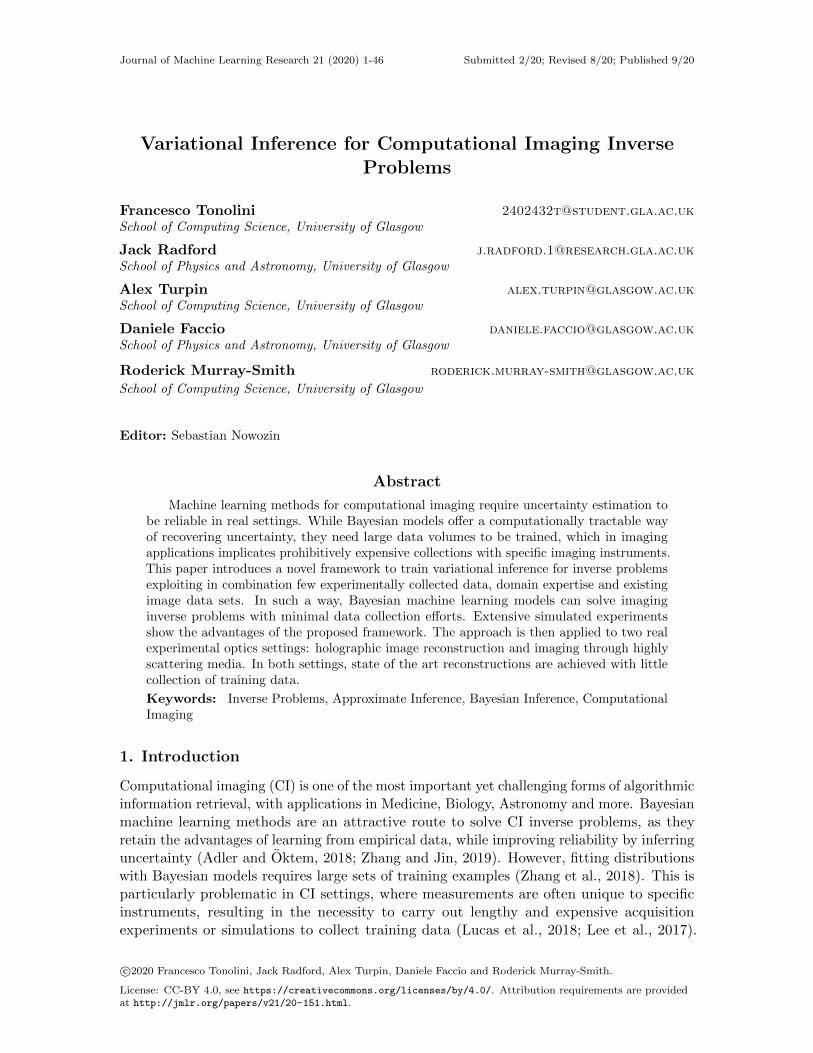
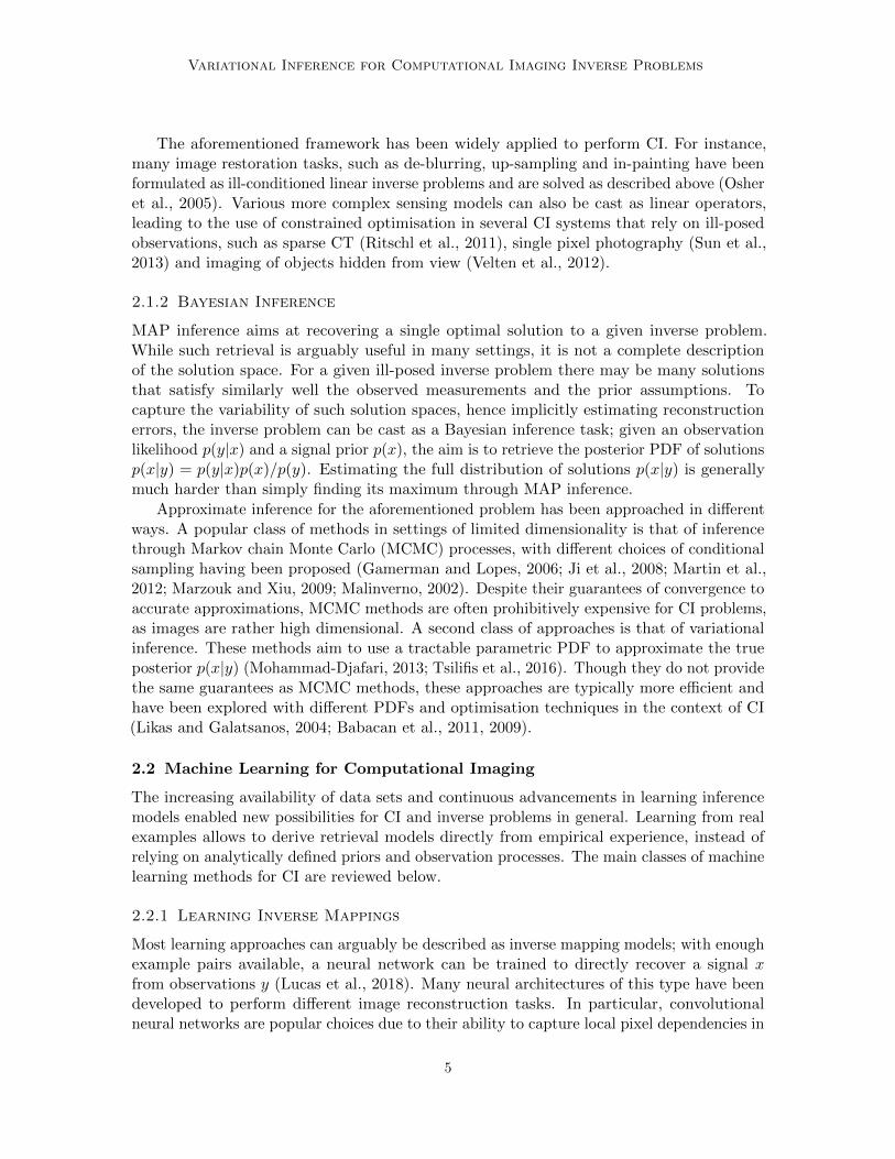
Figure 1: Proposed framework for training variational inference with diverse sources ofinformation accessible in imaging settings. (a) Firstly, a multi-fidelity forwardmodel is built to generate experimental observations. A variational model istrained to reproduce experimental observations Y ∗ from experimental groundtruth targets X∗, exploiting simulated predictions y given by some analyticalobservation model defined with domain expertise. (b) A CVAE then learns to solvethe inverse problem from a large data set of target examples X with a trainingloop; target examples x are passed through the previously learned multi-fidelityforward model to generate measurements y, which are then used as conditionsfor training the CVAE to generate back the targets x. In this way, a largenumber of ground truth targets can be exploited for learning, without the needfor associated experimental measurements. (c) The trained CVAE can then beused to draw different possible solutions xj,i to the inverse problem conditionedon a new observation yj .
Consider, for example, the task of reconstructing three dimensional environments fromLIDAR measurements. Applying machine learning to this task requires data, in particular,paired examples of 3D environments and signals recorded with the particular LIDAR systemto be employed. This means that, in principle, each LIDAR system being developed for thistask requires its own extensive data set of paired examples to be collected, rendering the useof machine learning extremely impractical.
This paper introduces a novel framework to train conditional variational models forsolving CI inverse problems leveraging in combination (i) a minimal amount of experimentallyacquired or numerically simulated ground truth target-observation pairs, (ii) an inexpensiveanalytical model of the observation process from domain expertise and (iii) a large numberof unobserved target examples, which can often be found in existing data sets. In such away, trained variational inference models benefit from all accessible useful data as well asdomain expertise, rather than relying solely on specifically collected training inputs andoutputs. Recalling the LIDAR example given above, the proposed method would allow
2
Variational Inference for Computational Imaging Inverse Problems
the joint utilisation of limited collections with the specific LIDAR instrument, a physicalmodel of LIDAR acquisition and any number of available examples of 3D environments totrain our machine learning models. The framework is derived with Bayesian formulations,interpreting the different sources of information available as samples from or approximationsto the underlying hidden distributions.
To address the expected scarcity of experimental data, the novel training strategyadopts a variational semi-supervision approach. Similarly to recent works in semi-supervisedVAEs, an auxiliary model is employed to map abundantly available target ground-truths tocorresponding measurements, which are, in contrast, scarce (Kingma et al., 2014; Maaløeet al., 2016; Nalisnick et al., 2019). However, the proposed framework introduces twoimportant differences, specifically adapting to CI problems:
i This auxiliary function incorporates a physical observation model designed with domainexpertise. In most imaging settings, the Physics of how targets map to correspondingmeasurements is well understood and described by closed form expressions. These shouldbe used to improve the quality of a reconstruction system.
ii Instead of training the two models simultaneously, a forward model is trained firstand then employed as a sampler in training the reconstruction model. This choice ismade to avoid that synthetic measurements, i.e. predicted by the auxiliary system,contain more information about the targets than those encountered in reality. Whilethis is not a critical problem for most semi-supervised systems, as auxiliary models oftenpredict low-dimensional conditions such as labels, it very much arises in imaging settings,where these conditions are instead measurements that have comparable or even higherdimensionality than the targets. This high dimensionality of the conditions allows asystem training the two models jointly to pass rich information through the syntheticmeasurements in order to maximise training reconstruction likelihood. By training theforward process separately instead, this auxiliary model is induced to maximise fidelityto real measurements alone, essentially providing an emulator.
Figure 1 schematically illustrate the framework and its components.The proposed framework is first quantitatively evaluated in simulated image recovery
experiments, making use of the benchmark data sets CelebA and CIFAR10 (Liu et al., 2015;Krizhevsky, 2009). In these experiments, different common transformations are applied to theimages, including Gaussian blurring, partial occlusion and down-sampling. Image recovery isthen performed with variational models. The novel training framework proved significantlyadvantageous across the range of tested conditions compared with standard training strategies.Secondly, the proposed technique is implemented with experimental imaging systems in twodifferent settings; phase-less holographic image reconstruction (Shechtman et al., 2015; Sinhaet al., 2017) and imaging through highly scattering media with temporally resolved sensors(Jiang, 2018; Lyons et al., 2019). In both settings, state of the art results are obtained withthe proposed technique, while requiring minimal experimental collection efforts for training.
2. Background and Related Work
Computational imaging (CI) broadly identifies a class of methods in which an image ofinterest is not directly observed, but rather inferred algorithmically from one or more
3
Tonolini, Radford, Turpin, Faccio and Murray-Smith
measurements (Bertero and Boccacci, 1998). Many image recovery tasks fall within thisdefinition, such as de-convolution (Starck et al., 2003; Bioucas-Dias et al., 2006), computedtomography (CT) (Ritschl et al., 2011) and structured illumination imaging (Magalhaeset al., 2011). Traditionally, CI tasks are modelled as inverse problems, where a target signalx ∈ Rn is measured through a forward model y = f(x), yielding observations y ∈ Rm. Theaim is then to retrieve the signal x from the observations y (Bertero and Boccacci, 1998;Vogel, 2002). In the following subsections, the main advances in solving imaging inverseproblems are reviewed and the relevant background on Bayesian multi-fidelity models iscovered.
2.1 Linear models and Hand-crafted Priors
In many CI problems, the forward observation model can be approximately described as alinear operator A ∈ Rm×n and some independent noise ε ∈ Rm (Bertero and Boccacci, 1998;Daubechies et al., 2004), such that the measurements y are assumed to be generated as
y = Ax+ ε. (1)
The noise ε often follows simple statistics, such as Gaussian or Bernoulli distributions,depending on the instruments and imaging settings. This choice of forward model iscomputationally advantageous for retrieval algorithms, as it can be run efficiently througha simple linear projection, and is often a sufficiently good approximation to the “true”observation process. The difficulty in retrieving the observed signal x from an observation yin this context derives from the fact that in CI inverse problems the operator A is often poorlyconditioned and consequentially the resulting inverse problem is ill-posed. Put differently,the inverse A−1 is not well-defined and small errors in y result in large errors in the naiveestimation x ' A−1y. To overcome this issue, the classical approach is to formulate certainprior assumptions about the nature of the target x that help in regularising its retrieval.
2.1.1 Maximum a Posteriori Inference
A widely adopted framework is that of maximum a posteriori (MAP) inference with ana-lytically defined prior assumptions. The aim is to find a solution which satisfies the linearobservations well, while imposing some properties which the target x is expected to retain.Under Gaussian noise assumptions, the estimate of x is recovered by solving a minimisationproblem of the form
arg minx
1
2||Ax− y||2 + λh(x), (2)
where || · || indicates the Euclidean norm, λ is a real positive parameter that controls theweight given to the regularisation and h(x) is an analytically defined penalty function thatenforces some desired property in x. In the case of images, it is common to assume that x issparse in some basis, such as frequency or wavelets, leading to `1-norm penalty functions(Daubechies et al., 2004; Donoho, 2006; Figueiredo et al., 2007). For such choices of penalty,and other common ones, the objective function of equation 2 is convex. This makes theoptimisation problem solvable with a variety of efficient methods (Daubechies et al., 2004;Yang and Zhang, 2011) and provides theoretical guarantees on the recoverability of thesolution (Candes et al., 2006).
4
Variational Inference for Computational Imaging Inverse Problems
The aforementioned framework has been widely applied to perform CI. For instance,many image restoration tasks, such as de-blurring, up-sampling and in-painting have beenformulated as ill-conditioned linear inverse problems and are solved as described above (Osheret al., 2005). Various more complex sensing models can also be cast as linear operators,leading to the use of constrained optimisation in several CI systems that rely on ill-posedobservations, such as sparse CT (Ritschl et al., 2011), single pixel photography (Sun et al.,2013) and imaging of objects hidden from view (Velten et al., 2012).
2.1.2 Bayesian Inference
MAP inference aims at recovering a single optimal solution to a given inverse problem.While such retrieval is arguably useful in many settings, it is not a complete descriptionof the solution space. For a given ill-posed inverse problem there may be many solutionsthat satisfy similarly well the observed measurements and the prior assumptions. Tocapture the variability of such solution spaces, hence implicitly estimating reconstructionerrors, the inverse problem can be cast as a Bayesian inference task; given an observationlikelihood p(y|x) and a signal prior p(x), the aim is to retrieve the posterior PDF of solutionsp(x|y) = p(y|x)p(x)/p(y). Estimating the full distribution of solutions p(x|y) is generallymuch harder than simply finding its maximum through MAP inference.
Approximate inference for the aforementioned problem has been approached in differentways. A popular class of methods in settings of limited dimensionality is that of inferencethrough Markov chain Monte Carlo (MCMC) processes, with different choices of conditionalsampling having been proposed (Gamerman and Lopes, 2006; Ji et al., 2008; Martin et al.,2012; Marzouk and Xiu, 2009; Malinverno, 2002). Despite their guarantees of convergence toaccurate approximations, MCMC methods are often prohibitively expensive for CI problems,as images are rather high dimensional. A second class of approaches is that of variationalinference. These methods aim to use a tractable parametric PDF to approximate the trueposterior p(x|y) (Mohammad-Djafari, 2013; Tsilifis et al., 2016). Though they do not providethe same guarantees as MCMC methods, these approaches are typically more efficient andhave been explored with different PDFs and optimisation techniques in the context of CI(Likas and Galatsanos, 2004; Babacan et al., 2011, 2009).
2.2 Machine Learning for Computational Imaging
The increasing availability of data sets and continuous advancements in learning inferencemodels enabled new possibilities for CI and inverse problems in general. Learning from realexamples allows to derive retrieval models directly from empirical experience, instead ofrelying on analytically defined priors and observation processes. The main classes of machinelearning methods for CI are reviewed below.
2.2.1 Learning Inverse Mappings
Most learning approaches can arguably be described as inverse mapping models; with enoughexample pairs available, a neural network can be trained to directly recover a signal xfrom observations y (Lucas et al., 2018). Many neural architectures of this type have beendeveloped to perform different image reconstruction tasks. In particular, convolutionalneural networks are popular choices due to their ability to capture local pixel dependencies in
5
Tonolini, Radford, Turpin, Faccio and Murray-Smith
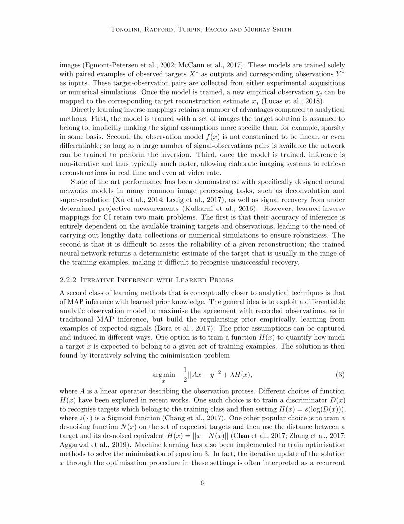
images (Egmont-Petersen et al., 2002; McCann et al., 2017). These models are trained solelywith paired examples of observed targets X∗ as outputs and corresponding observations Y ∗
as inputs. These target-observation pairs are collected from either experimental acquisitionsor numerical simulations. Once the model is trained, a new empirical observation yj can bemapped to the corresponding target reconstruction estimate xj (Lucas et al., 2018).
Directly learning inverse mappings retains a number of advantages compared to analyticalmethods. First, the model is trained with a set of images the target solution is assumed tobelong to, implicitly making the signal assumptions more specific than, for example, sparsityin some basis. Second, the observation model f(x) is not constrained to be linear, or evendifferentiable; so long as a large number of signal-observations pairs is available the networkcan be trained to perform the inversion. Third, once the model is trained, inference isnon-iterative and thus typically much faster, allowing elaborate imaging systems to retrievereconstructions in real time and even at video rate.
State of the art performance has been demonstrated with specifically designed neuralnetworks models in many common image processing tasks, such as deconvolution andsuper-resolution (Xu et al., 2014; Ledig et al., 2017), as well as signal recovery from underdetermined projective measurements (Kulkarni et al., 2016). However, learned inversemappings for CI retain two main problems. The first is that their accuracy of inference isentirely dependent on the available training targets and observations, leading to the need ofcarrying out lengthy data collections or numerical simulations to ensure robustness. Thesecond is that it is difficult to asses the reliability of a given reconstruction; the trainedneural network returns a deterministic estimate of the target that is usually in the range ofthe training examples, making it difficult to recognise unsuccessful recovery.
2.2.2 Iterative Inference with Learned Priors
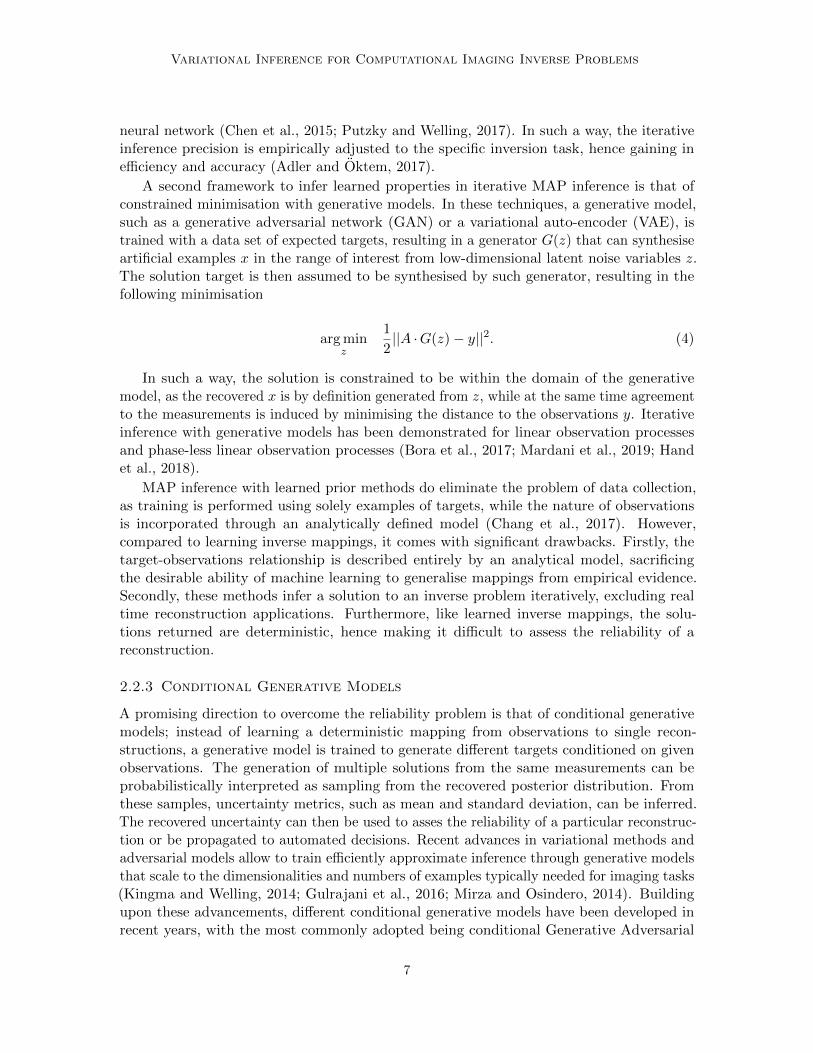
A second class of learning methods that is conceptually closer to analytical techniques is thatof MAP inference with learned prior knowledge. The general idea is to exploit a differentiableanalytic observation model to maximise the agreement with recorded observations, as intraditional MAP inference, but build the regularising prior empirically, learning fromexamples of expected signals (Bora et al., 2017). The prior assumptions can be capturedand induced in different ways. One option is to train a function H(x) to quantify how mucha target x is expected to belong to a given set of training examples. The solution is thenfound by iteratively solving the minimisation problem
arg minx
1
2||Ax− y||2 + λH(x), (3)
where A is a linear operator describing the observation process. Different choices of functionH(x) have been explored in recent works. One such choice is to train a discriminator D(x)to recognise targets which belong to the training class and then setting H(x) = s(log(D(x))),where s( · ) is a Sigmoid function (Chang et al., 2017). One other popular choice is to train ade-noising function N(x) on the set of expected targets and then use the distance between atarget and its de-noised equivalent H(x) = ||x−N(x)|| (Chan et al., 2017; Zhang et al., 2017;Aggarwal et al., 2019). Machine learning has also been implemented to train optimisationmethods to solve the minimisation of equation 3. In fact, the iterative update of the solutionx through the optimisation procedure in these settings is often interpreted as a recurrent
6
Variational Inference for Computational Imaging Inverse Problems
neural network (Chen et al., 2015; Putzky and Welling, 2017). In such a way, the iterativeinference precision is empirically adjusted to the specific inversion task, hence gaining inefficiency and accuracy (Adler and Oktem, 2017).
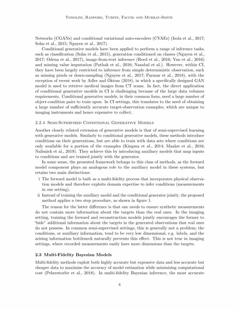
A second framework to infer learned properties in iterative MAP inference is that ofconstrained minimisation with generative models. In these techniques, a generative model,such as a generative adversarial network (GAN) or a variational auto-encoder (VAE), istrained with a data set of expected targets, resulting in a generator G(z) that can synthesiseartificial examples x in the range of interest from low-dimensional latent noise variables z.The solution target is then assumed to be synthesised by such generator, resulting in thefollowing minimisation
arg minz
1
2||A ·G(z)− y||2. (4)
In such a way, the solution is constrained to be within the domain of the generativemodel, as the recovered x is by definition generated from z, while at the same time agreementto the measurements is induced by minimising the distance to the observations y. Iterativeinference with generative models has been demonstrated for linear observation processesand phase-less linear observation processes (Bora et al., 2017; Mardani et al., 2019; Handet al., 2018).
MAP inference with learned prior methods do eliminate the problem of data collection,as training is performed using solely examples of targets, while the nature of observationsis incorporated through an analytically defined model (Chang et al., 2017). However,compared to learning inverse mappings, it comes with significant drawbacks. Firstly, thetarget-observations relationship is described entirely by an analytical model, sacrificingthe desirable ability of machine learning to generalise mappings from empirical evidence.Secondly, these methods infer a solution to an inverse problem iteratively, excluding realtime reconstruction applications. Furthermore, like learned inverse mappings, the solu-tions returned are deterministic, hence making it difficult to assess the reliability of areconstruction.
2.2.3 Conditional Generative Models
A promising direction to overcome the reliability problem is that of conditional generativemodels; instead of learning a deterministic mapping from observations to single recon-structions, a generative model is trained to generate different targets conditioned on givenobservations. The generation of multiple solutions from the same measurements can beprobabilistically interpreted as sampling from the recovered posterior distribution. Fromthese samples, uncertainty metrics, such as mean and standard deviation, can be inferred.The recovered uncertainty can then be used to asses the reliability of a particular reconstruc-tion or be propagated to automated decisions. Recent advances in variational methods andadversarial models allow to train efficiently approximate inference through generative modelsthat scale to the dimensionalities and numbers of examples typically needed for imaging tasks(Kingma and Welling, 2014; Gulrajani et al., 2016; Mirza and Osindero, 2014). Buildingupon these advancements, different conditional generative models have been developed inrecent years, with the most commonly adopted being conditional Generative Adversarial
7
Tonolini, Radford, Turpin, Faccio and Murray-Smith
Networks (CGANs) and conditional variational auto-encoders (CVAEs) (Isola et al., 2017;Sohn et al., 2015; Nguyen et al., 2017).
Conditional generative models have been applied to perform a range of inference tasks,such as classification (Sohn et al., 2015), generation conditioned on classes (Nguyen et al.,2017; Odena et al., 2017), image-from-text inference (Reed et al., 2016; Yan et al., 2016)and missing value imputation (Pathak et al., 2016; Nazabal et al.). However, within CI,they have been largely restricted to inference from simple deterministic observation, suchas missing pixels or down-sampling (Nguyen et al., 2017; Parmar et al., 2018), with theexception of recent work by Adler and Oktem (2018), in which a specifically designed GANmodel is used to retrieve medical images from CT scans. In fact, the direct applicationof conditional generative models in CI is challenging because of the large data volumesrequirements. Conditional generative models, in their common form, need a large number ofobject-condition pairs to train upon. In CI settings, this translates to the need of obtaininga large number of sufficiently accurate target-observation examples, which are unique toimaging instruments and hence expensive to collect.
2.2.4 Semi-Supervised Conditional Generative Models
Another closely related extension of generative models is that of semi-supervised learningwith generative models. Similarly to conditional generative models, these methods introduceconditions on their generations, but are able to train with data sets where conditions areonly available for a portion of the examples (Kingma et al., 2014; Maaløe et al., 2016;Nalisnick et al., 2019). They achieve this by introducing auxiliary models that map inputsto conditions and are trained jointly with the generator.
In some sense, the presented framework belongs to this class of methods, as the forwardmodel component plays an analogous role to the auxiliary model in these systems, butretains two main distinctions:
i The forward model is built as a multi-fidelity process that incorporates physical observa-tion models and therefore exploits domain expertise to infer conditions (measurementsin our setting).
ii Instead of training the auxiliary model and the conditional generator jointly, the proposedmethod applies a two step procedure, as shown in figure 1.
The reason for the latter difference is that one needs to ensure synthetic measurementsdo not contain more information about the targets than the real ones. In the imagingsetting, training the forward and reconstruction models jointly encourages the former to“hide” additional information about the targets in the generated observations that real onesdo not possess. In common semi-supervised settings, this is generally not a problem; theconditions, or auxiliary information, tend to be very low dimensional, e.g. labels, and thearising information bottleneck naturally prevents this effect. This is not true in imagingsettings, where recorded measurements easily have more dimensions than the targets.
2.3 Multi-Fidelity Bayesian Models
Multi-fidelity methods exploit both highly accurate but expensive data and less accurate butcheaper data to maximise the accuracy of model estimation while minimising computationalcost (Peherstorfer et al., 2018). In multi-fidelity Bayesian inference, the most accurate
8
Variational Inference for Computational Imaging Inverse Problems
predictions, or high-fidelity outputs, are considered to be draws from the underlying truedensity of interest and the aim is to approximately recover such high-fidelity outputs fromthe corresponding inputs and low-fidelity outputs of some cheaper computation (Kaipioand Somersalo, 2007). Within Bayesian approaches to solve inverse problems, multi-fidelitymodels have been used to minimise the cost of estimating expensive forward processes, inparticular with MCMC methods to efficiently estimate the likelihood at each sampling step(Christen and Fox, 2005).
In Bayesian optimisation settings, the difference between high and low fidelity predictionsis commonly modeled with Gaussian processes, where approximate function evaluations aremade cheap by computing low-fidelity estimates and subsequently mapping them to high-fidelity estimates with a Gaussian process (Kennedy and O’Hagan, 2001; Bayarri et al., 2007).In CI settings, Gaussian process multi-fidelity models are difficult to apply, as the availablevolume of data and the dimensionality of the targets and observations are potentially verylarge. Recent work by Yang and Perdikaris (2019) proposes to model high-fidelity data withconditional deep generative models, which are instead capable of scaling to the volumesand dimensionalities needed in imaging applications. The multi-fidelity component of theframework presented here follows these ideas and exploits a deep CVAE to model highfidelity data when inferring an accurate forward observation process.
3. Variational Framework for Imaging Inverse Problems
Differently from previous approaches, the proposed variational framework is built to learnfrom all the useful data and models typically available in CI problems. In the followingsubsections the problem of Bayesian learning in this context is defined and the componentsof the proposed variational learning method are derived and motivated.
3.1 Problem Description
3.1.1 The Bayesian Inverse Problem
The aim of computational imaging is to recover a hidden target xj ∈ RN from someassociated observed measurements yj ∈ RM . In the Bayesian formulation, the measurementsyj are assumed to be drawn from an observation distribution p(y|xj) and the objective is todetermine the posterior p(x|yj); the distribution of all possible reconstructions. FollowingBayes’ rule, the form of this posterior is
p(x|yj) =p(yj |x)p(x)
p(yj). (5)
The observation distribution p(y|x), often referred to as the data likelihood, describes theobservation process, mapping targets to measurements. Given any ground truth targetxi the corresponding measurements that are physically recorded yi are draws from thedata likelihood yi ∼ p(y|xi). The prior distribution p(x) models the assumed knowledgeabout the targets of interest. This PDF is the distribution of possible targets prior tocarrying out any measurement. Finally, the marginal likelihood p(y) =
∫p(x)p(y|x)dx is
the distribution of all possible measurements y. The goal of variational inference is to learna non-iterative approximation to the true intractable posterior distribution of equation 5 for
9
Tonolini, Radford, Turpin, Faccio and Murray-Smith
arbitrary new observations yj . That is, learning a parametric distribution rθ(x|y) which wellapproximates the true posterior p(x|y) for any new observation yj ∼ p(y) and from whichone can non-iteratively draw possible reconstructions xj,i ∼ rθ(x|yj).
3.1.2 Information Available
For a given imaging inverse problem of the type described above, there are generally threemain sources of information that can be exploited to obtain the best estimate of the targetposterior. The first is empirical observations. Physical experiments to collect sets of ground-truth targets X∗ ∈ RN×K and associated observations Y ∗ ∈ RM×K can be recorded with theimaging apparatus of interest. The number of these acquisitions K is normally limited bythe time and effort necessary for experimental preparation and collection, or alternatively bycomputational cost, if these are obtained through numerical simulations. However, empiricaltarget-observation pairs are the most accurate evaluation of the true observation process andtherefore can be very informative. A recorded observation yk ∈ Y ∗ obtained when imaginga target xk ∈ X∗ can be interpreted as a sample from the true data likelihood yk ∼ p(y|xk).
The second source of information is domain expertise. The measurement process, mappingtargets to observations, is described by a physical phenomenon. With knowledge of suchphenomenon, one can construct a functional mapping, normally referred to as forward model,which computes observations’ estimates y from targets x. For instance, many observationprocesses in CI settings can be approximately modelled by a linear transformation andindependent Gaussian or Poisson noise (Daubechies et al., 2004). It is clearly infeasible toobtain analytical models that perfectly match reality. However, an analytical forward modelcan provide inexpensive approximations y to the true observations y that can be computedfor any target x. In the Bayesian formulation, a forward model can be interpreted as aclosed form approximation p(y|x) to the true data likelihood p(y|x).
Lastly, many examples of the targets of interest X ∈ RN×L are often available in theform of unlabelled data sets. Because collection of this type of data is independent of theimaging apparatus, the number of available examples L is expected to be much greater thanthe number of empirical acquisitions K. In fact, many large image data sets containingrelevant targets for CI applications are readily available and easily accessible. These targetexamples xl ∈ X can be interpreted as draws from the prior distribution xl ∼ p(x). Insummary, the available sources of information are
• Limited sets of ground-truth targets X∗ = {xk=1:K} and associated observationsY ∗ = {yk=1:K}, the elements of which are point samples of the true data likelihoodyk ∼ p(y|xk).
• An analytical forward model providing a closed form approximation for the true datalikelihood p(y|x) ≈ p(y|x).
• A large set of target examples X = {xl=1:L} corresponding to prior samples xl ∼ p(x),where L� K.
The scope of this paper is to design a framework for learning the best possible approximatedistribution rθ(x|y) by exploiting all the available sources of information described above.
10
Variational Inference for Computational Imaging Inverse Problems
3.2 Multi-Fidelity Forward Modelling
Before training the inversion, an approximate observation distribution pα(y|x) is trained tofit the true data likelihood p(y|x). Learning this observation distribution first allows effectiveincorporation of domain expertise, as in CI problems this is usually available in the formof an analytical forward model. Furthermore, training the observation model is expectedto require far fewer training input-output pairs than training the corresponding inversion,as most forward models are well-posed, while the corresponding inverse problems are oftenill-posed. A good approximation to the data likelihood pα(y|x) can therefore be learnedwith a much lower number K of experimental ground-truth targets X∗ and measurementsY ∗ than would be required to train a good approximate posterior rθ(x|y) directly.
In order to make use of the analytical approximation p(y|x), hence incorporating domainexpertise in the training procedure, the approximate observation distribution is chosen as
pα(y|x) =
∫p(y|x)pα(y|x, y)dy. (6)
In such a way, the inference of a measurement y, a high-fidelity prediction, from a target xcan exploit the output y of the analytical forward model p(y|x), which instead is considereda low-fidelity prediction. The parametric component to be trained is then the conditionalpα(y|x, y), which returns high-fidelity sample measurements y from targets x and low-fidelitypredictions y.
To provide flexible inference in the general case, the PDF pα(y|x, y) is chosen to be alatent variable model of the form
pα(y|x, y) =
∫pα1(w|x, y)pα2(y|x, y, w)dw. (7)
The two parametric distributions pα1(w|x, y) and pα2(y|x, y, w) are chosen to be Gaussiandistributions, the moments of which are outputs of neural networks with weights α1 andα2 respectively.1 The model of equation 6 is then trained to fit the sets of experimentalground-truth targets and measurements X∗ and Y ∗, as these are point samples of thetrue data likelihood of interest yk ∼ p(y|xk). The optimisation to be performed is the loglikelihood maximisation
arg maxα1,α2
log pα(Y ∗|X∗) =K∑k=1
log
∫p(y|xk)
∫pα1(w|xk, y)pα2(yk|xk, y, w)dwdy. (8)
Due to the integration over latent variables w, the maximisation of equation 8 is intractable todirectly perform stochastically. However, problems of this type can be approximately solvedefficiently with a variational auto-encoding approach, in which a parametric recognitionmodel is used as a sampling function (Kingma and Welling, 2014; Sohn et al., 2015). TheVAE formulation for the multi-fidelity model is presented in detail in supplementary sectionA.1. Through this approach, training of the parameters α = {α1, α2} and β can be performedthrough the following stochastic optimisation:
arg maxα1,α2,β
K∑k=1
V∑v=1
[S∑s=1
log pα2(yk|xk, yv, ws)−DKL(qβ(w|xk, yk, yv)||pα1(w|xk, yv))
]. (9)
1. The distribution pα2(y|x, y, w) can alternatively be chosen to match some other noise model if theobservation noise is known to be of a particular type, such as Poisson or Bernoulli.
11
Tonolini, Radford, Turpin, Faccio and Murray-Smith
1
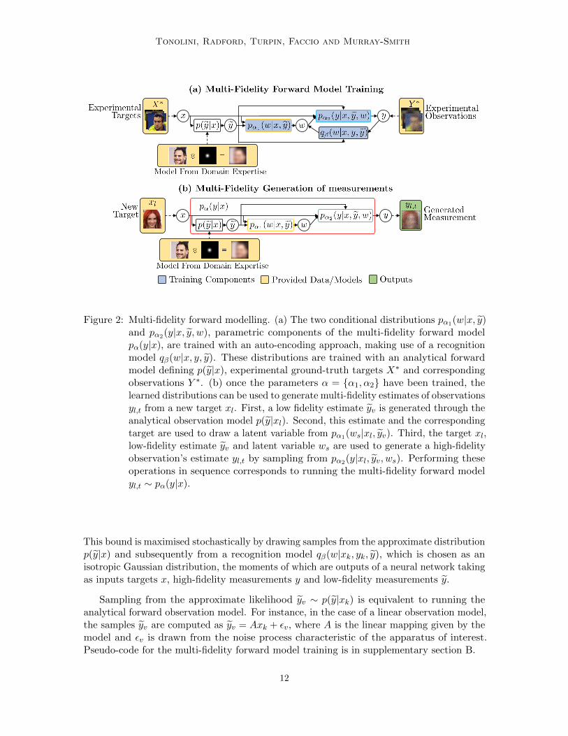
Figure 2: Multi-fidelity forward modelling. (a) The two conditional distributions pα1(w|x, y)and pα2(y|x, y, w), parametric components of the multi-fidelity forward modelpα(y|x), are trained with an auto-encoding approach, making use of a recognitionmodel qβ(w|x, y, y). These distributions are trained with an analytical forwardmodel defining p(y|x), experimental ground-truth targets X∗ and correspondingobservations Y ∗. (b) once the parameters α = {α1, α2} have been trained, thelearned distributions can be used to generate multi-fidelity estimates of observationsyl,t from a new target xl. First, a low fidelity estimate yv is generated through theanalytical observation model p(y|xl). Second, this estimate and the correspondingtarget are used to draw a latent variable from pα1(ws|xl, yv). Third, the target xl,low-fidelity estimate yv and latent variable ws are used to generate a high-fidelityobservation’s estimate yl,t by sampling from pα2(y|xl, yv, ws). Performing theseoperations in sequence corresponds to running the multi-fidelity forward modelyl,t ∼ pα(y|x).
This bound is maximised stochastically by drawing samples from the approximate distributionp(y|x) and subsequently from a recognition model qβ(w|xk, yk, y), which is chosen as anisotropic Gaussian distribution, the moments of which are outputs of a neural network takingas inputs targets x, high-fidelity measurements y and low-fidelity measurements y.
Sampling from the approximate likelihood yv ∼ p(y|xk) is equivalent to running theanalytical forward observation model. For instance, in the case of a linear observation model,the samples yv are computed as yv = Axk + εv, where A is the linear mapping given by themodel and εv is drawn from the noise process characteristic of the apparatus of interest.Pseudo-code for the multi-fidelity forward model training is in supplementary section B.
12
Variational Inference for Computational Imaging Inverse Problems
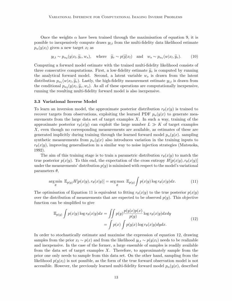
Once the weights α have been trained through the maximisation of equation 9, it ispossible to inexpensively compute draws yl,t from the multi-fidelity data likelihood estimatepα(y|xl) given a new target xl as
yl,t ∼ pα2(y|xl, yv, ws), where yv ∼ p(y|xl) and ws ∼ pα1(w|xl, yv). (10)
Computing a forward model estimate with the trained multi-fidelity likelihood consists ofthree consecutive computations. First, a low-fidelity estimate yv is computed by runningthe analytical forward model. Second, a latent variable ws is drawn from the latentdistribution pα1(w|xl, yv). Lastly, the high-fidelity measurement estimate yl,t is drawn fromthe conditional pα2(y|xl, yv, ws). As all of these operations are computationally inexpensive,running the resulting multi-fidelity forward model is also inexpensive.
3.3 Variational Inverse Model
To learn an inversion model, the approximate posterior distribution rθ(x|y) is trained torecover targets from observations, exploiting the learned PDF pα(y|x) to generate mea-surements from the large data set of target examples X. In such a way, training of theapproximate posterior rθ(x|y) can exploit the large number L � K of target examplesX, even though no corresponding measurements are available, as estimates of these aregenerated implicitly during training through the learned forward model pα(y|x). samplingsynthetic measurements from pα(y|x) also introduces variation in the training inputs torθ(x|y), improving generalisation in a similar way to noise injection strategies (Matsuoka,1992).
The aim of this training stage is to train a parametric distribution rθ(x|y) to match thetrue posterior p(x|y). To this end, the expectation of the cross entropy H[p(x|y), rθ(x|y)]under the measurements’ distribution p(y) is minimised with respect to the model’s variationalparameters θ,
arg minθ
Ep(y)H[p(x|y), rθ(x|y)] = arg maxθ
Ep(y)∫p(x|y) log rθ(x|y)dx. (11)
The optimisation of Equation 11 is equivalent to fitting rθ(x|y) to the true posterior p(x|y)over the distribution of measurements that are expected to be observed p(y). This objectivefunction can be simplified to give
Ep(y)∫p(x|y) log rθ(x|y)dx =
∫∫p(y)
p(y|x)p(x)
p(y)log rθ(x|y)dxdy
=
∫p(x)
∫p(y|x) log rθ(x|y)dydx.
(12)
In order to stochastically estimate and maximise the expression of equation 12, drawingsamples from the prior xl ∼ p(x) and from the likelihood yl,t ∼ p(y|xl) needs to be realizableand inexpensive. In the case of the former, a large ensemble of samples is readily availablefrom the data set of target examples X. Therefore, to approximately sample from theprior one only needs to sample from this data set. On the other hand, sampling from thelikelihood p(y|xl) is not possible, as the form of the true forward observation model is notaccessible. However, the previously learned multi-fidelity forward model pα(y|x), described
13
Tonolini, Radford, Turpin, Faccio and Murray-Smith
in subsection 3.2, offers a learned approximation to the data likelihood from which it isinexpensive to draw realisations. The objective of equation 12 to be maximised can then beapproximated as
Ep(y)∫p(x|y) log rθ(x|y)dx '
∫p(x)
∫pα(y|x) log rθ(x|y)dydx. (13)
In this form, stochastic estimation is inexpensive, as prior samples xl ∼ p(x) can be drawnfrom the data set X and draws from the approximate likelihood yl,t ∼ pα(y|xl) can becomputed by running the multi-fidelity forward model as described in subsection 3.2.
3.3.1 CVAE as Approximate Posterior
The approximate distribution rθ(x|y) needs to be of considerable capacity in order toaccurately capture the variability of solution spaces in imaging inverse problems. To thisend, the approximating distribution rθ(x|y) is chosen as a conditional latent variable model
rθ(x|y) =
∫rθ1(z|y)rθ2(x|z, y)dz. (14)
The latent distribution rθ1(z|y) is an isotropic Gaussian distribution N (z;µz, σ2z), where its
moments µz and σ2z are inferred from a measurement y by a neural network. The neuralnetworks may be convolutional or fully connected, depending on the nature of the observedsignal from which images need to be reconstructed. The likelihood distribution rθ2(x|z, y) cantake different forms, depending on the nature of the images to be recovered and requirementson the efficiency of training and reconstruction. In the experiments presented here, thedistribution rθ2(x|z, y) was set to either an isotropic Gaussian with moments determined bya fully connected neural network, taking concatenated z and y as input, or a convolutionalpixel conditional model analogous to that of a pixelVAE (Gulrajani et al., 2016).
Latent variable models of this type have been proven to be powerful conditional imagegenerators (Sohn et al., 2015; Nguyen et al., 2017) and therefore are expected to be suitablevariational approximators for posteriors in imaging problems. With this choice of approximateposterior rθ(x|y), the objective function for model training is
arg maxθ1,θ2
∫p(x)
∫pα(y|x) log
∫rθ1(z|y)rθ2(x|z, y)dzdydx. (15)
As for the likelihood structure in the multi-fidelity forward modelling, directly performingthe maximisation of equation 15 is intractable due to the integral over the latent spacevariables z. However, using Jensen’s inequality, a tractable lower bound for this expressioncan be derived with the aid of a parametric recognition model qφ(z|x, y).
As for the forward multi-fidelity model, the recognition model qφ(z|x, y) is an isotropicGaussian distribution in the latent space, with moments inferred by a neural network, takingas input both example targets x and corresponding observations y. This neural networkmay be fully connected, partly convolutional or completely convolutional, depending on thenature of the targets x and observations y. The VAE formulation for the Variational inverseproblem is presented in detail in supplementary section A.2. Making use of this lower bound,
14
Variational Inference for Computational Imaging Inverse Problems
1
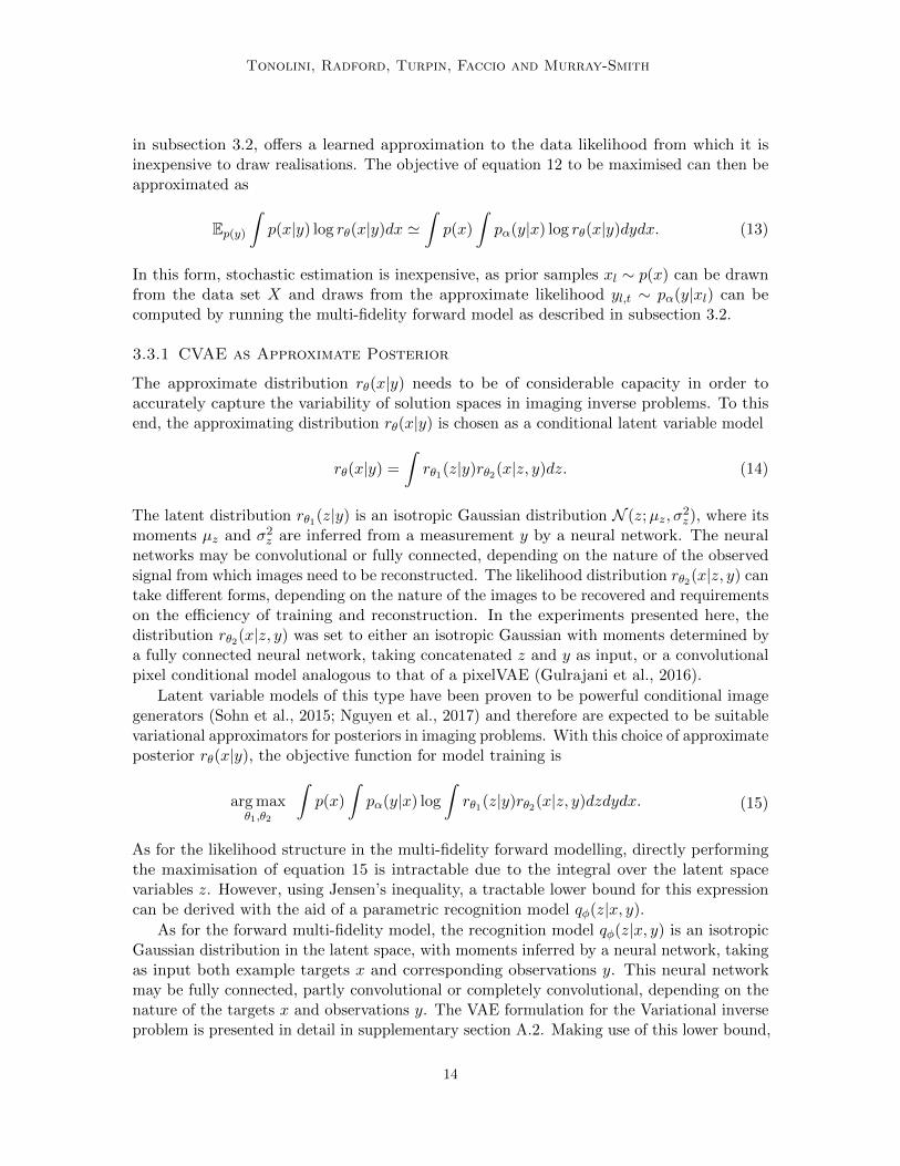
Figure 3: Variational inverse model. (a) The model is trained to maximise the evidencelower bound on the likelihood of targets x conditioned on observations y. Theposterior components rθ1(z|y) and rθ2(x|z, y) are trained along with the auxiliaryrecognition model qφ(z|x, y). Instead of training on paired targets and conditions,as for standard CVAEs, the model is given target examples X alone and generatestraining conditions y stochastically through the previously learned multi-fidelityforward model pα(y|x). (b) Given new observations yj , samples from the approxi-mate posterior rθ(x|yj) can be non-iteratively generated with the trained modelby first drawing a latent variable zj,i ∼ rθ1(z|yj) and subsequently generating atarget xj,i ∼ rθ2(x|zj,i, yj).
we can define the objective function for the inverse model as
arg maxθ1,θ2,φ
L∑l=1
T∑t=1
[S∑s=1
log rθ2(xl|zs, yl,t)−DKL(qφ(z|xl, yl,t)||rθ1(z|yl,t))
], (16)
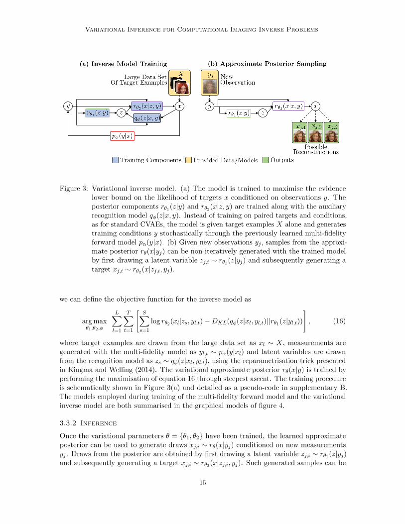
where target examples are drawn from the large data set as xl ∼ X, measurements aregenerated with the multi-fidelity model as yl,t ∼ pα(y|xl) and latent variables are drawnfrom the recognition model as zs ∼ qφ(z|xl, yl,t), using the reparametrisation trick presentedin Kingma and Welling (2014). The variational approximate posterior rθ(x|y) is trained byperforming the maximisation of equation 16 through steepest ascent. The training procedureis schematically shown in Figure 3(a) and detailed as a pseudo-code in supplementary B.The models employed during training of the multi-fidelity forward model and the variationalinverse model are both summarised in the graphical models of figure 4.
3.3.2 Inference
Once the variational parameters θ = {θ1, θ2} have been trained, the learned approximateposterior can be used to generate draws xj,i ∼ rθ(x|yj) conditioned on new measurementsyj . Draws from the posterior are obtained by first drawing a latent variable zj,i ∼ rθ1(z|yj)and subsequently generating a target xj,i ∼ rθ2(x|zj,i, yj). Such generated samples can be
15
Tonolini, Radford, Turpin, Faccio and Murray-Smith
Figure 4: Graphical models for training of the multi-fidelity forward model and the varia-tional inverse model.
interpreted as different possible solutions to the inverse problem and can be used in differentways to extract information of interest. For instance, one can compute per-pixel marginalmeans and standard deviations, in order to visualise the expected mean values and marginaluncertainty on the retrieved images. Figure 3(b) schematically illustrates the approximateposterior sampling procedure.
It may be of interest to also estimate a single best retrieval x∗j given the observedmeasurements yj , which would be the image yielding the highest likelihood rθ(x
∗j |yj). This
retrieval can be performed iteratively, by maximising rθ(x|yj) with respect to x, as proposedby Sohn et al. (2015). As the focus of this work is non-iterative inference, a pseudo-maximumnon-iterative retrieval is instead used. Such retrieval is performed by considering the pointof maximum likelihood of the conditional Gaussian distribution in the latent space rθ1(z|yj),which is by definition its mean µz,j . The pseudo-maximum reconstruction x∗j is then the pointof maximum likelihood of rθ2(x|µz,j , yj), which is also its mean µx,j . This pseudo-maximumestimate adds the ability to retrieve an inexpensive near-optimal reconstruction, analogousto that recovered by deterministic mappings.
4. Experiments
The proposed framework is tested both in simulation and with real imaging systems.Firstly, quantitative simulated experiments are performed to compare the proposed trainingframework to other strategies using the same Bayesian networks. Secondly, the new approachis applied to phase-less holographic image reconstruction and imaging through highlyscattering media, comparing reconstructions to the most recent state of the art in therespective fields.
4.1 Simulated Experiments
Simple image restoration tasks are performed in simulation. Experiments include Gaussianblurring, down-sampling and partial occlusion with both CelebA and CIFAR examples (Liuet al., 2015; Krizhevsky, 2009). The test images are corrupted with the given transformationand additive Gaussian noise. Variational models are then used to perform reconstructions,
16
Variational Inference for Computational Imaging Inverse Problems
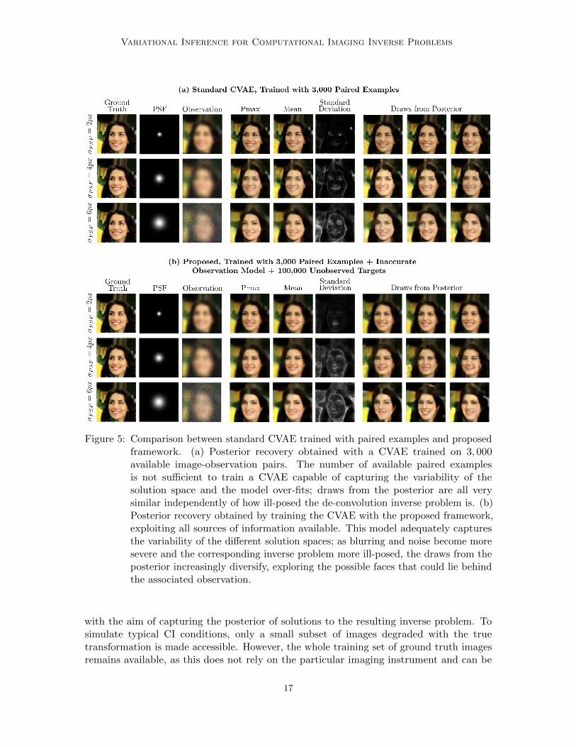
Figure 5: Comparison between standard CVAE trained with paired examples and proposedframework. (a) Posterior recovery obtained with a CVAE trained on 3, 000available image-observation pairs. The number of available paired examplesis not sufficient to train a CVAE capable of capturing the variability of thesolution space and the model over-fits; draws from the posterior are all verysimilar independently of how ill-posed the de-convolution inverse problem is. (b)Posterior recovery obtained by training the CVAE with the proposed framework,exploiting all sources of information available. This model adequately capturesthe variability of the different solution spaces; as blurring and noise become moresevere and the corresponding inverse problem more ill-posed, the draws from theposterior increasingly diversify, exploring the possible faces that could lie behindthe associated observation.
with the aim of capturing the posterior of solutions to the resulting inverse problem. Tosimulate typical CI conditions, only a small subset of images degraded with the truetransformation is made accessible. However, the whole training set of ground truth imagesremains available, as this does not rely on the particular imaging instrument and can be
17
Tonolini, Radford, Turpin, Faccio and Murray-Smith
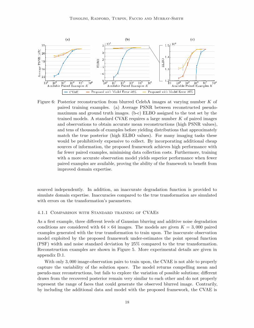
Figure 6: Posterior reconstruction from blurred CelebA images at varying number K ofpaired training examples. (a) Average PSNR between reconstructed pseudo-maximum and ground truth images. (b-c) ELBO assigned to the test set by thetrained models. A standard CVAE requires a large number K of paired imagesand observations to obtain accurate mean reconstructions (high PSNR values),and tens of thousands of examples before yielding distributions that approximatelymatch the true posterior (high ELBO values). For many imaging tasks thesewould be prohibitively expensive to collect. By incorporating additional cheapsources of information, the proposed framework achieves high performance withfar fewer paired examples, minimising data collection costs. Furthermore, trainingwith a more accurate observation model yields superior performance when fewerpaired examples are available, proving the ability of the framework to benefit fromimproved domain expertise.
sourced independently. In addition, an inaccurate degradation function is provided tosimulate domain expertise. Inaccuracies compared to the true transformation are simulatedwith errors on the transformation’s parameters.
4.1.1 Comparison with Standard training of CVAEs
As a first example, three different levels of Gaussian blurring and additive noise degradationconditions are considered with 64 × 64 images. The models are given K = 3, 000 pairedexamples generated with the true transformation to train upon. The inaccurate observationmodel exploited by the proposed framework under-estimates the point spread function(PSF) width and noise standard deviation by 25% compared to the true transformation.Reconstruction examples are shown in Figure 5. More experimental details are given inappendix D.1.
With only 3, 000 image-observation pairs to train upon, the CVAE is not able to properlycapture the variability of the solution space. The model returns compelling mean andpseudo-max reconstructions, but fails to explore the variation of possible solutions; differentdraws from the recovered posterior remain very similar to each other and do not properlyrepresent the range of faces that could generate the observed blurred image. Contrarily,by including the additional data and model with the proposed framework, the CVAE is
18
Variational Inference for Computational Imaging Inverse Problems
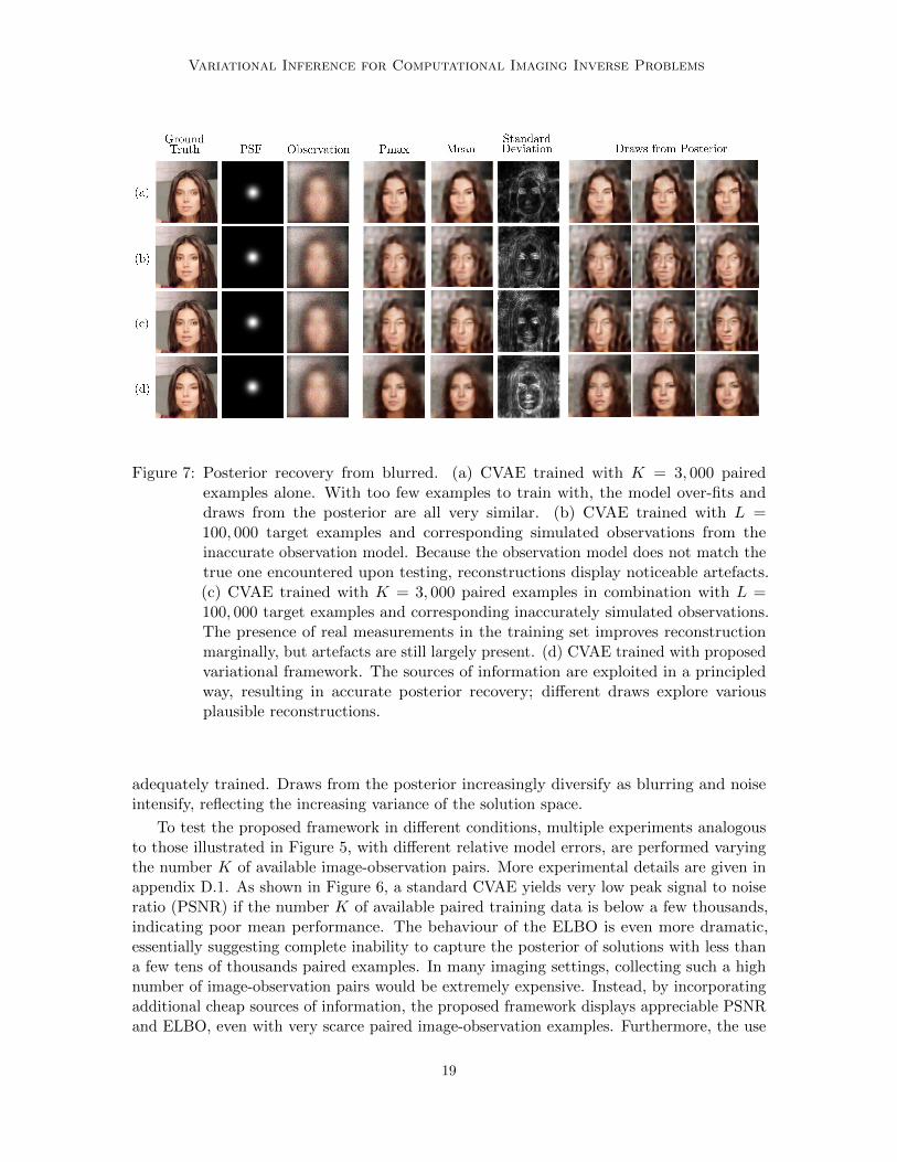
Figure 7: Posterior recovery from blurred. (a) CVAE trained with K = 3, 000 pairedexamples alone. With too few examples to train with, the model over-fits anddraws from the posterior are all very similar. (b) CVAE trained with L =100, 000 target examples and corresponding simulated observations from theinaccurate observation model. Because the observation model does not match thetrue one encountered upon testing, reconstructions display noticeable artefacts.(c) CVAE trained with K = 3, 000 paired examples in combination with L =100, 000 target examples and corresponding inaccurately simulated observations.The presence of real measurements in the training set improves reconstructionmarginally, but artefacts are still largely present. (d) CVAE trained with proposedvariational framework. The sources of information are exploited in a principledway, resulting in accurate posterior recovery; different draws explore variousplausible reconstructions.
adequately trained. Draws from the posterior increasingly diversify as blurring and noiseintensify, reflecting the increasing variance of the solution space.
To test the proposed framework in different conditions, multiple experiments analogousto those illustrated in Figure 5, with different relative model errors, are performed varyingthe number K of available image-observation pairs. More experimental details are given inappendix D.1. As shown in Figure 6, a standard CVAE yields very low peak signal to noiseratio (PSNR) if the number K of available paired training data is below a few thousands,indicating poor mean performance. The behaviour of the ELBO is even more dramatic,essentially suggesting complete inability to capture the posterior of solutions with less thana few tens of thousands paired examples. In many imaging settings, collecting such a highnumber of image-observation pairs would be extremely expensive. Instead, by incorporatingadditional cheap sources of information, the proposed framework displays appreciable PSNRand ELBO, even with very scarce paired image-observation examples. Furthermore, the use
19
Tonolini, Radford, Turpin, Faccio and Murray-Smith
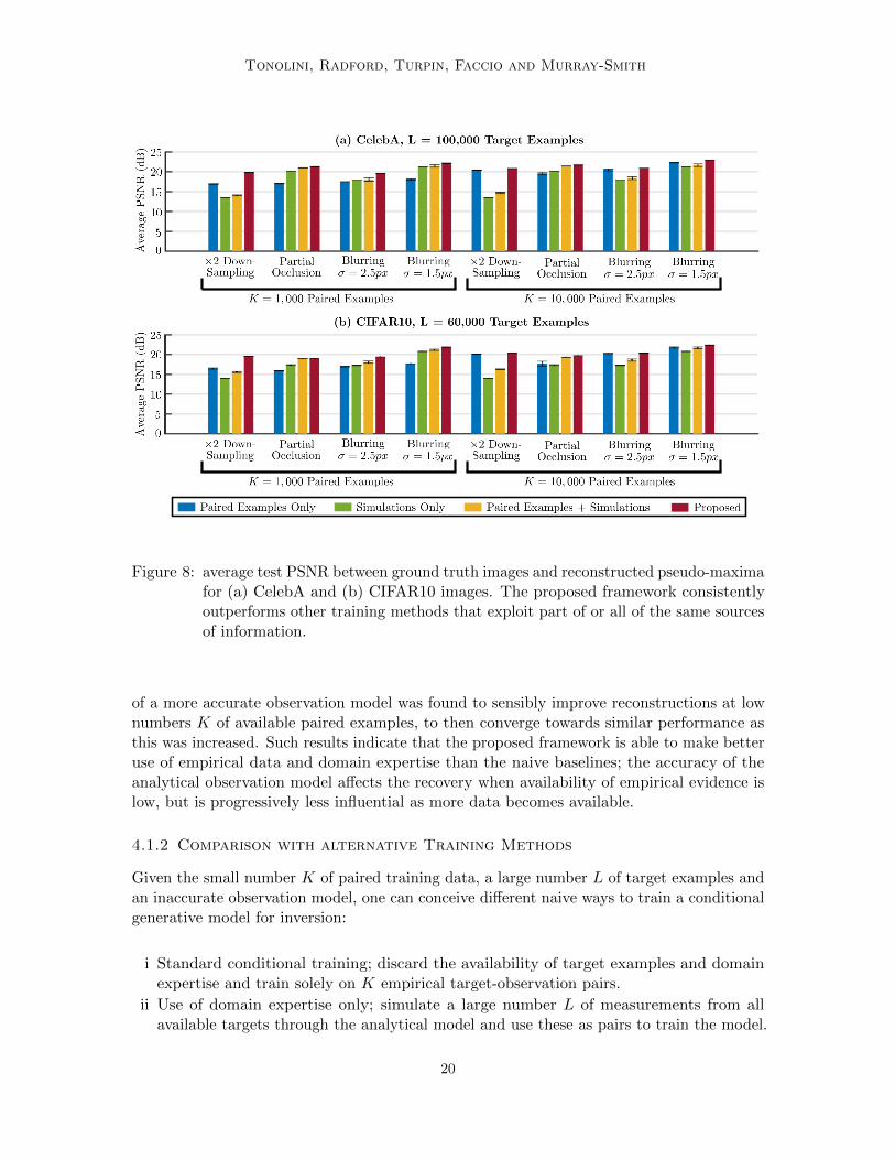
Figure 8: average test PSNR between ground truth images and reconstructed pseudo-maximafor (a) CelebA and (b) CIFAR10 images. The proposed framework consistentlyoutperforms other training methods that exploit part of or all of the same sourcesof information.
of a more accurate observation model was found to sensibly improve reconstructions at lownumbers K of available paired examples, to then converge towards similar performance asthis was increased. Such results indicate that the proposed framework is able to make betteruse of empirical data and domain expertise than the naive baselines; the accuracy of theanalytical observation model affects the recovery when availability of empirical evidence islow, but is progressively less influential as more data becomes available.
4.1.2 Comparison with alternative Training Methods
Given the small number K of paired training data, a large number L of target examples andan inaccurate observation model, one can conceive different naive ways to train a conditionalgenerative model for inversion:
i Standard conditional training; discard the availability of target examples and domainexpertise and train solely on K empirical target-observation pairs.
ii Use of domain expertise only; simulate a large number L of measurements from allavailable targets through the analytical model and use these as pairs to train the model.
20
Variational Inference for Computational Imaging Inverse Problems
Laser
DMD
Fourier lens
Camera
Image at DMD Image at camera
Fourier transform
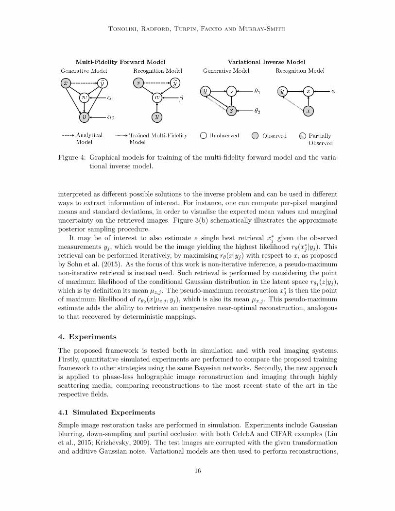
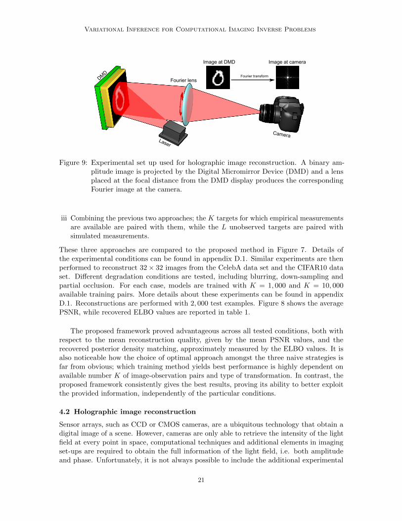
Figure 9: Experimental set up used for holographic image reconstruction. A binary am-plitude image is projected by the Digital Micromirror Device (DMD) and a lensplaced at the focal distance from the DMD display produces the correspondingFourier image at the camera.
iii Combining the previous two approaches; the K targets for which empirical measurementsare available are paired with them, while the L unobserved targets are paired withsimulated measurements.
These three approaches are compared to the proposed method in Figure 7. Details ofthe experimental conditions can be found in appendix D.1. Similar experiments are thenperformed to reconstruct 32× 32 images from the CelebA data set and the CIFAR10 dataset. Different degradation conditions are tested, including blurring, down-sampling andpartial occlusion. For each case, models are trained with K = 1, 000 and K = 10, 000available training pairs. More details about these experiments can be found in appendixD.1. Reconstructions are performed with 2, 000 test examples. Figure 8 shows the averagePSNR, while recovered ELBO values are reported in table 1.
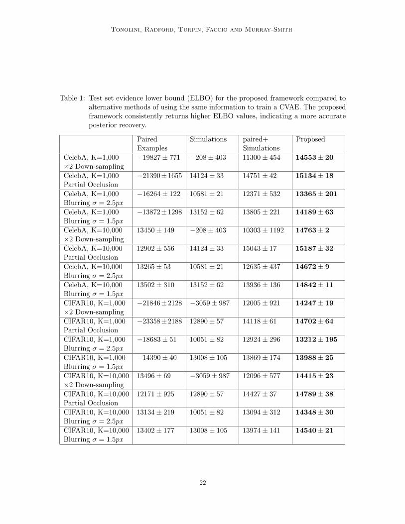
The proposed framework proved advantageous across all tested conditions, both withrespect to the mean reconstruction quality, given by the mean PSNR values, and therecovered posterior density matching, approximately measured by the ELBO values. It isalso noticeable how the choice of optimal approach amongst the three naive strategies isfar from obvious; which training method yields best performance is highly dependent onavailable number K of image-observation pairs and type of transformation. In contrast, theproposed framework consistently gives the best results, proving its ability to better exploitthe provided information, independently of the particular conditions.
4.2 Holographic image reconstruction
Sensor arrays, such as CCD or CMOS cameras, are a ubiquitous technology that obtain adigital image of a scene. However, cameras are only able to retrieve the intensity of the lightfield at every point in space, computational techniques and additional elements in imagingset-ups are required to obtain the full information of the light field, i.e. both amplitudeand phase. Unfortunately, it is not always possible to include the additional experimental
21
Tonolini, Radford, Turpin, Faccio and Murray-Smith
Table 1: Test set evidence lower bound (ELBO) for the proposed framework compared toalternative methods of using the same information to train a CVAE. The proposedframework consistently returns higher ELBO values, indicating a more accurateposterior recovery.
Paired Simulations paired+ ProposedExamples Simulations
CelebA, K=1,000 −19827± 771 −208± 403 11300± 454 14553± 20×2 Down-sampling
CelebA, K=1,000 −21390±1655 14124± 33 14751± 42 15134± 18Partial Occlusion
CelebA, K=1,000 −16264± 122 10581± 21 12371± 532 13365± 201Blurring σ = 2.5px
CelebA, K=1,000 −13872±1298 13152± 62 13805± 221 14189± 63Blurring σ = 1.5px
CelebA, K=10,000 13450± 149 −208± 403 10303± 1192 14763± 2×2 Down-sampling
CelebA, K=10,000 12902± 556 14124± 33 15043± 17 15187± 32Partial Occlusion
CelebA, K=10,000 13265± 53 10581± 21 12635± 437 14672± 9Blurring σ = 2.5px
CelebA, K=10,000 13502± 310 13152± 62 13936± 136 14842± 11Blurring σ = 1.5px
CIFAR10, K=1,000 −21846±2128 −3059± 987 12005± 921 14247± 19×2 Down-sampling
CIFAR10, K=1,000 −23358±2188 12890± 57 14118± 61 14702± 64Partial Occlusion
CIFAR10, K=1,000 −18683± 51 10051± 82 12924± 296 13212± 195Blurring σ = 2.5px
CIFAR10, K=1,000 −14390± 40 13008± 105 13869± 174 13988± 25Blurring σ = 1.5px
CIFAR10, K=10,000 13496± 69 −3059± 987 12096± 577 14415± 23×2 Down-sampling
CIFAR10, K=10,000 12171± 925 12890± 57 14427± 37 14789± 38Partial Occlusion
CIFAR10, K=10,000 13134± 219 10051± 82 13094± 312 14348± 30Blurring σ = 2.5px
CIFAR10, K=10,000 13402± 177 13008± 105 13974± 141 14540± 21Blurring σ = 1.5px
22
Variational Inference for Computational Imaging Inverse Problems
components to the set-up and therefore algorithms have been adapted to use only intensityimages. Retrieving the full light field information from intensity-only measurements is avery important inverse problem that has been studied exhaustively during the last 40 years(Gerchberg, 1972; Fienup, 1982; Shechtman et al., 2015).
Machine learning methods have been proposed in this context to learn either phase oramplitude of images/light fields from intensity-only diffraction patterns recorded with acamera (Sinha et al., 2017; Rivenson et al., 2018, 2019). Such an ability is desirable becausethe intensity images can be recorded with cheap digital cameras, instead of expensive anddelicate phase-sensitive instruments. Following these recent advances, we aim to use ourproposed variational framework approach to solve the following problem: Given the cameraintensity image of the diffraction pattern at the Fourier plane, what is the amplitude of thecorresponding projected image? This apparently simple problem has multiple applications inareas such as material science, where X-rays are used to infer the structure of a molecule fromits diffraction pattern (Marchesini et al., 2003; Barmherzig et al., 2019), optical trapping(Jesacher et al., 2008), and microscopy (Faulkner and Rodenburg, 2004).
4.2.1 Experimental set-up and Data
The experiment consisted of an expanded laser beam incident onto a Digital MicromirrorDevice (DMD) which displays binary patterns, as shown in Figure 9. DMDs consist of anarray of micron-sized mirrors that can be arranged into two angles that correspond to “on”and “off” states of the micromirror. Consequently, the amplitude of the light is binarisedby the DMD pattern and propagates toward a single lens. The lens, placed at the focaldistance from the DMD display, will cause the rays to form the Fourier image of the MNISTdigit at the camera.
To make the problem even harder, we work under saturation conditions, i.e. assumingblinding on the camera, and with extremely low-resolution images. We display 9600 MNISTdigits on the DMD and record the corresponding camera observations. This data is used ashigh fidelity paired ground truths X∗ and measurements Y ∗. The remaining 50400 MNISTexamples are used as the large set of unobserved ground truth signals X. The analyticalobservation model p(y|x) is built as a simple intensity Fourier transform computation, towhich we add artificial saturation.
4.2.2 Reconstruction
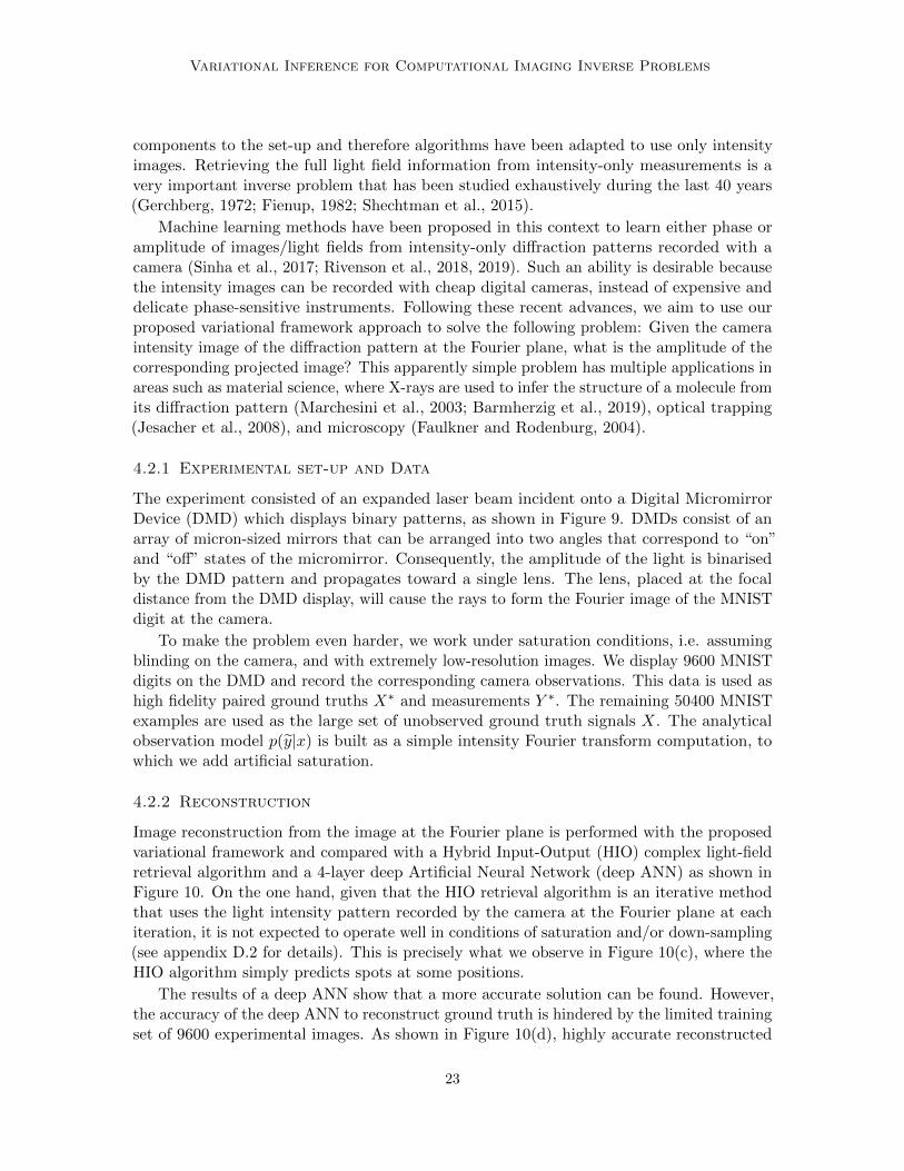
Image reconstruction from the image at the Fourier plane is performed with the proposedvariational framework and compared with a Hybrid Input-Output (HIO) complex light-fieldretrieval algorithm and a 4-layer deep Artificial Neural Network (deep ANN) as shown inFigure 10. On the one hand, given that the HIO retrieval algorithm is an iterative methodthat uses the light intensity pattern recorded by the camera at the Fourier plane at eachiteration, it is not expected to operate well in conditions of saturation and/or down-sampling(see appendix D.2 for details). This is precisely what we observe in Figure 10(c), where theHIO algorithm simply predicts spots at some positions.
The results of a deep ANN show that a more accurate solution can be found. However,the accuracy of the deep ANN to reconstruct ground truth is hindered by the limited trainingset of 9600 experimental images. As shown in Figure 10(d), highly accurate reconstructed
23
Tonolini, Radford, Turpin, Faccio and Murray-Smith
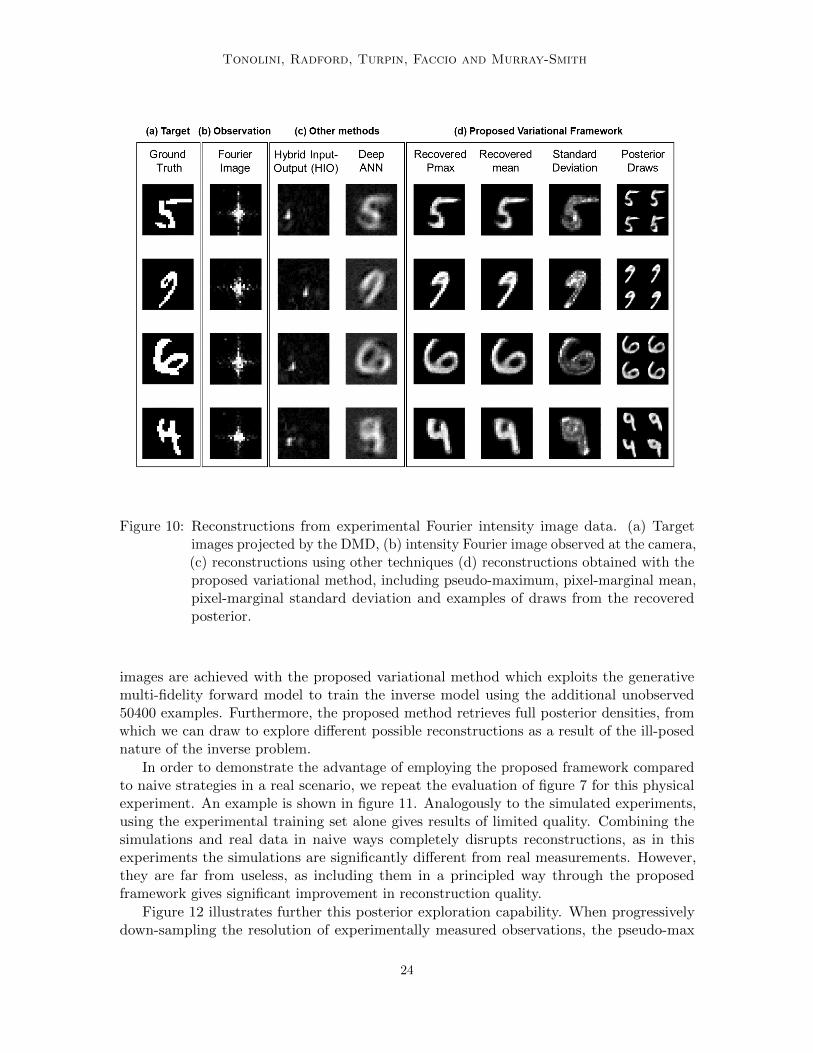
Figure 10: Reconstructions from experimental Fourier intensity image data. (a) Targetimages projected by the DMD, (b) intensity Fourier image observed at the camera,(c) reconstructions using other techniques (d) reconstructions obtained with theproposed variational method, including pseudo-maximum, pixel-marginal mean,pixel-marginal standard deviation and examples of draws from the recoveredposterior.
images are achieved with the proposed variational method which exploits the generativemulti-fidelity forward model to train the inverse model using the additional unobserved50400 examples. Furthermore, the proposed method retrieves full posterior densities, fromwhich we can draw to explore different possible reconstructions as a result of the ill-posednature of the inverse problem.
In order to demonstrate the advantage of employing the proposed framework comparedto naive strategies in a real scenario, we repeat the evaluation of figure 7 for this physicalexperiment. An example is shown in figure 11. Analogously to the simulated experiments,using the experimental training set alone gives results of limited quality. Combining thesimulations and real data in naive ways completely disrupts reconstructions, as in thisexperiments the simulations are significantly different from real measurements. However,they are far from useless, as including them in a principled way through the proposedframework gives significant improvement in reconstruction quality.
Figure 12 illustrates further this posterior exploration capability. When progressivelydown-sampling the resolution of experimentally measured observations, the pseudo-max
24
Variational Inference for Computational Imaging Inverse Problems
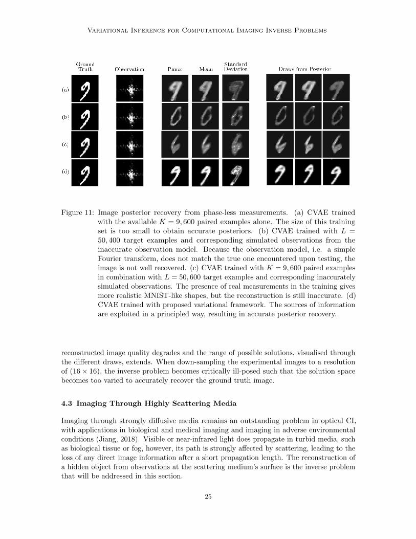
Figure 11: Image posterior recovery from phase-less measurements. (a) CVAE trainedwith the available K = 9, 600 paired examples alone. The size of this trainingset is too small to obtain accurate posteriors. (b) CVAE trained with L =50, 400 target examples and corresponding simulated observations from theinaccurate observation model. Because the observation model, i.e. a simpleFourier transform, does not match the true one encountered upon testing, theimage is not well recovered. (c) CVAE trained with K = 9, 600 paired examplesin combination with L = 50, 600 target examples and corresponding inaccuratelysimulated observations. The presence of real measurements in the training givesmore realistic MNIST-like shapes, but the reconstruction is still inaccurate. (d)CVAE trained with proposed variational framework. The sources of informationare exploited in a principled way, resulting in accurate posterior recovery.
reconstructed image quality degrades and the range of possible solutions, visualised throughthe different draws, extends. When down-sampling the experimental images to a resolutionof (16× 16), the inverse problem becomes critically ill-posed such that the solution spacebecomes too varied to accurately recover the ground truth image.
4.3 Imaging Through Highly Scattering Media
Imaging through strongly diffusive media remains an outstanding problem in optical CI,with applications in biological and medical imaging and imaging in adverse environmentalconditions (Jiang, 2018). Visible or near-infrared light does propagate in turbid media, suchas biological tissue or fog, however, its path is strongly affected by scattering, leading to theloss of any direct image information after a short propagation length. The reconstruction ofa hidden object from observations at the scattering medium’s surface is the inverse problemthat will be addressed in this section.
25
Tonolini, Radford, Turpin, Faccio and Murray-Smith
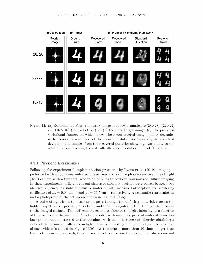
Figure 12: (a) Experimental Fourier intensity image data down-sampled to (28×28), (22×22)and (16× 16) (top to bottom) for (b) the same target image. (c) The proposedvariational framework which shows the reconstructed image quality degradeswith decreasing resolution of the measured data. As expected, the standarddeviation and samples from the recovered posterior show high variability to thesolution when reaching the critically ill-posed resolution limit of (16× 16).
4.3.1 Physical Experiment
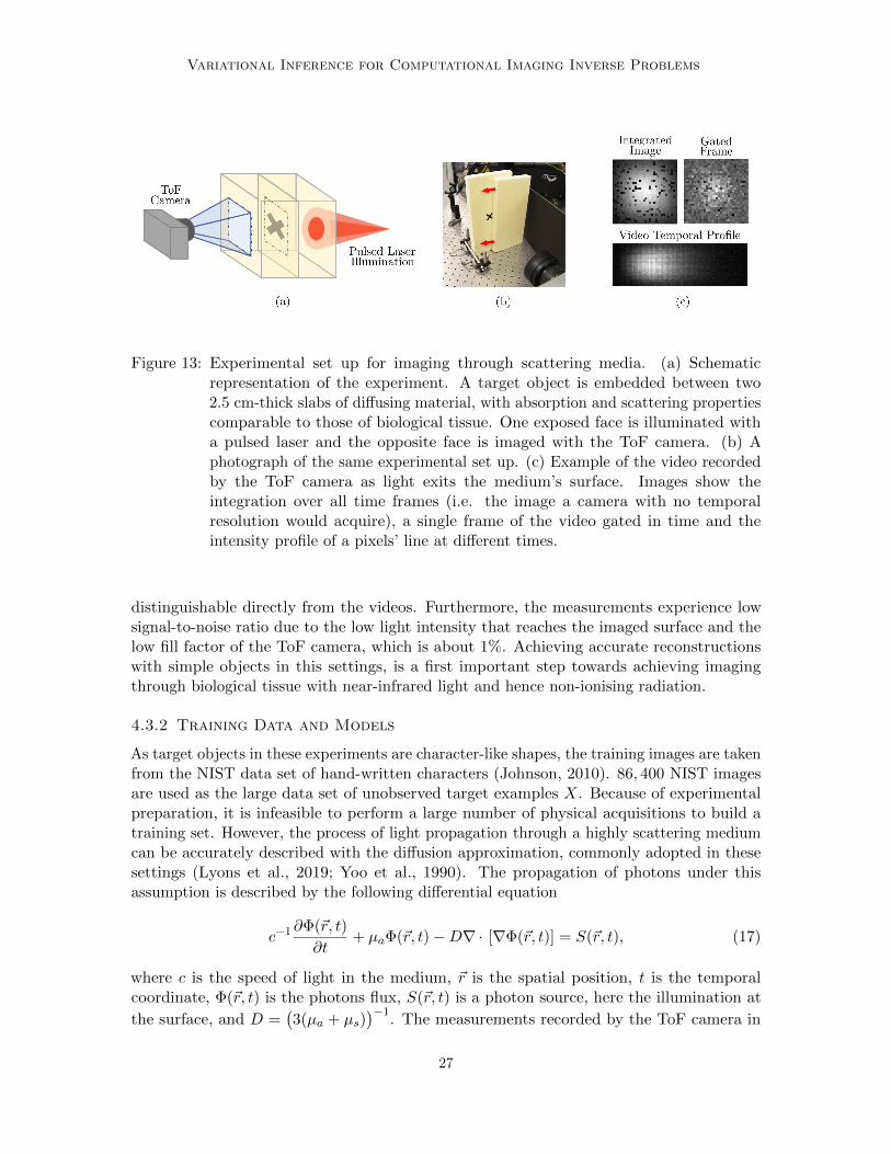
Following the experimental implementation presented by Lyons et al. (2019), imaging isperformed with a 130 fs near-infrared pulsed laser and a single photon sensitive time of flight(ToF) camera with a temporal resolution of 55 ps to perform transmission diffuse imaging.In these experiments, different cut-out shapes of alphabetic letters were placed between twoidentical 2.5 cm thick slabs of diffusive material, with measured absorption and scatteringcoefficients of µa = 0.09 cm−1 and µs = 16.5 cm−1 respectively. A schematic representationand a photograph of the set up are shown in Figure 13(a-b).
A pulse of light from the laser propagates through the diffusing material, reaches thehidden object, which partially absorbs it, and then propagates further through the mediumto the imaged surface. The ToF camera records a video of the light intensity as a functionof time as it exits the medium. A video recorded with an empty piece of material is used asbackground and subtracted to that obtained with the object present, thereby obtaining avideo of the estimated difference in light intensity caused by the hidden object. An exampleof such videos is shown in Figure 13(c). At this depth, more than 40 times longer thanthe photon’s mean free path, the diffusion effect is so severe that even basic shapes are not
26
Variational Inference for Computational Imaging Inverse Problems
Figure 13: Experimental set up for imaging through scattering media. (a) Schematicrepresentation of the experiment. A target object is embedded between two2.5 cm-thick slabs of diffusing material, with absorption and scattering propertiescomparable to those of biological tissue. One exposed face is illuminated witha pulsed laser and the opposite face is imaged with the ToF camera. (b) Aphotograph of the same experimental set up. (c) Example of the video recordedby the ToF camera as light exits the medium’s surface. Images show theintegration over all time frames (i.e. the image a camera with no temporalresolution would acquire), a single frame of the video gated in time and theintensity profile of a pixels’ line at different times.
distinguishable directly from the videos. Furthermore, the measurements experience lowsignal-to-noise ratio due to the low light intensity that reaches the imaged surface and thelow fill factor of the ToF camera, which is about 1%. Achieving accurate reconstructionswith simple objects in this settings, is a first important step towards achieving imagingthrough biological tissue with near-infrared light and hence non-ionising radiation.
4.3.2 Training Data and Models
As target objects in these experiments are character-like shapes, the training images are takenfrom the NIST data set of hand-written characters (Johnson, 2010). 86, 400 NIST imagesare used as the large data set of unobserved target examples X. Because of experimentalpreparation, it is infeasible to perform a large number of physical acquisitions to build atraining set. However, the process of light propagation through a highly scattering mediumcan be accurately described with the diffusion approximation, commonly adopted in thesesettings (Lyons et al., 2019; Yoo et al., 1990). The propagation of photons under thisassumption is described by the following differential equation
c−1∂Φ(~r, t)
∂t+ µaΦ(~r, t)−D∇ · [∇Φ(~r, t)] = S(~r, t), (17)
where c is the speed of light in the medium, ~r is the spatial position, t is the temporalcoordinate, Φ(~r, t) is the photons flux, S(~r, t) is a photon source, here the illumination at
the surface, and D =(3(µa + µs)
)−1. The measurements recorded by the ToF camera in
27
Tonolini, Radford, Turpin, Faccio and Murray-Smith
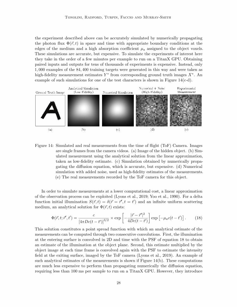
the experiment described above can be accurately simulated by numerically propagatingthe photon flux Φ(~r, t) in space and time with appropriate boundary conditions at theedges of the medium and a high absorption coefficient µa assigned to the object voxels.These simulations are accurate, but expensive. To simulate the experiments of interest herethey take in the order of a few minutes per example to run on a TitanX GPU. Obtainingpaired inputs and outputs for tens of thousands of experiments is expensive. Instead, only1, 000 examples of the 84, 400 training targets were generated in this way and were taken ashigh-fidelity measurement estimates Y ∗ from corresponding ground truth images X∗. Anexample of such simulations for one of the test characters is shown in Figure 14(c-d).
Figure 14: Simulated and real measurements from the time of flight (ToF) Camera. Imagesare single frames from the camera videos. (a) Image of the hidden object. (b) Sim-ulated measurement using the analytical solution from the linear approximation,taken as low-fidelity estimate. (c) Simulation obtained by numerically propa-gating the diffusion equation, which is accurate, but expensive. (d) Numericalsimulation with added noise, used as high-fidelity estimates of the measurements.(e) The real measurements recorded by the ToF camera for this object.
In order to simulate measurements at a lower computational cost, a linear approximationof the observation process can be exploited (Lyons et al., 2019; Yoo et al., 1990). For a deltafunction initial illumination S(~r, t) = δ(~r = ~r′, t = t′) and an infinite uniform scatteringmedium, an analytical solution for Φ(~r, t) exists:
Φ(~r, t;~r′, t′) =c
[4πDc(t− t′)]3/2× exp
[− |~r − ~r′|2
4Dc(t− t′)
]exp
[−µac(t− t′)
]. (18)
This solution constitutes a point spread function with which an analytical estimate of themeasurements can be computed through two consecutive convolutions. First, the illuminationat the entering surface is convolved in 2D and time with the PSF of equation 18 to obtainan estimate of the illumination at the object plane. Second, this estimate multiplied by theobject image at each time frame is convolved again with the PSF to estimate the intensityfield at the exiting surface, imaged by the ToF camera (Lyons et al., 2019). An example ofsuch analytical estimates of the measurements is shown if Figure 14(b). These computationsare much less expensive to perform than propagating numerically the diffusion equation,requiring less than 100 ms per sample to run on a TitanX GPU. However, they introduce
28
Variational Inference for Computational Imaging Inverse Problems
approximations which sacrifice the accuracy of the simulated measurements. In particular,they don’t take into account any boundary condition and assume that the observationprocess is linear, whereas in reality the light absorbed by some part of the object will affectthe illumination at some other part. This analytical observation model is taken as theapproximate likelihood p(y|x) generating low-fidelity measurement’s estimates y.
4.3.3 Results
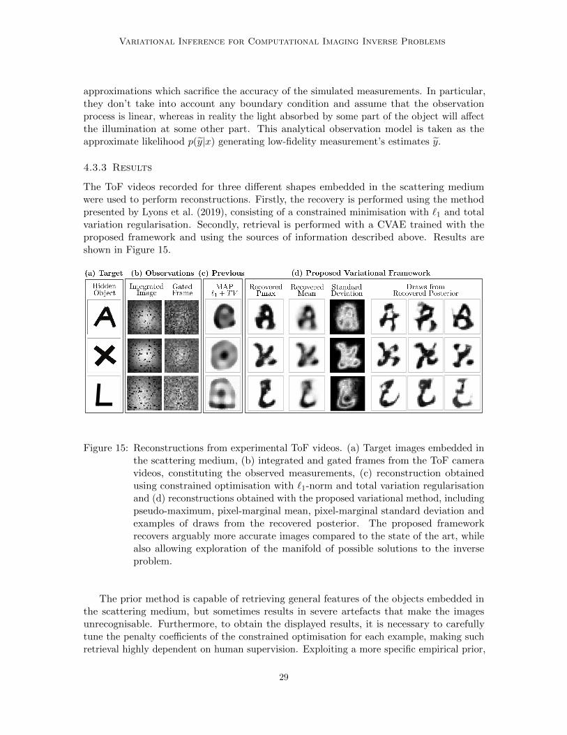
The ToF videos recorded for three different shapes embedded in the scattering mediumwere used to perform reconstructions. Firstly, the recovery is performed using the methodpresented by Lyons et al. (2019), consisting of a constrained minimisation with `1 and totalvariation regularisation. Secondly, retrieval is performed with a CVAE trained with theproposed framework and using the sources of information described above. Results areshown in Figure 15.
Figure 15: Reconstructions from experimental ToF videos. (a) Target images embedded inthe scattering medium, (b) integrated and gated frames from the ToF cameravideos, constituting the observed measurements, (c) reconstruction obtainedusing constrained optimisation with `1-norm and total variation regularisationand (d) reconstructions obtained with the proposed variational method, includingpseudo-maximum, pixel-marginal mean, pixel-marginal standard deviation andexamples of draws from the recovered posterior. The proposed frameworkrecovers arguably more accurate images compared to the state of the art, whilealso allowing exploration of the manifold of possible solutions to the inverseproblem.
The prior method is capable of retrieving general features of the objects embedded inthe scattering medium, but sometimes results in severe artefacts that make the imagesunrecognisable. Furthermore, to obtain the displayed results, it is necessary to carefullytune the penalty coefficients of the constrained optimisation for each example, making suchretrieval highly dependent on human supervision. Exploiting a more specific empirical prior,
29
Tonolini, Radford, Turpin, Faccio and Murray-Smith
the proposed framework allows to retrieve more accurate reconstructions, where the differentletters are clearly recognisable. Moreover, this particularly ill-posed inverse problem examplehighlights the importance of using a Bayesian approach; the solution space given a diffuseToF video is rather variable and, unlike constrained optimisation and other single estimatemethods, through the approximate posterior such variability can be captured by empiricallyestimating uncertainty and visualising different drawn samples, as shown in Figure 15(d).Note that, thanks to the proposed framework, the model was successfully trained with verylimited effort and resources; the large data set of targets was readily available independentlyof the application of interest, while only 1, 000 expensive simulations were used, requiringjust a few tens of hours of simulation time on a single GPU to be generated.
5. Conclusion
This paper introduced a novel framework to train variational inference in imaging inverseproblems, utilising different types of data and domain expertise in combination. As a result,Bayesian machine learning is rendered accessible for a broad range of imaging applications,where empirical training data is typically scarce or expensive to collect. The method wasderived from a Bayesian formulation of inverse problems and interpreting accessible sourcesof information as approximations to or samples from underlying distributions, providingtheoretical foundation. Simulated experiments thoroughly tested the proposed technique ina range of different conditions, proving its ability to better exploit all sources of informationavailable. The method was then applied to real imaging systems, demonstrating the firstsuccessful application of Bayesian machine learning in both phase-less holographic imagereconstruction and imaging through scattering media. In both settings, state of the artreconstructions were achieved, while requiring little training collection efforts, whereas beforeBayesian methods would have required prohibitively large volumes of data.
Acknowledgments
We would like to thank the editor and reviewers for their thoughtful, constructive anddetailed reviews which have improved the final paper. F.T., R.M-S., D.F. acknowledgefunding from Amazon and EPSRC grants EP/M01326X/1, EP/T00097X/1 (QuantIC, theUK Quantum Technology Hub in Quantum Enhanced Imaging) and EP/R018634/1 (Closed-Loop Data Science for Complex, Computationally- and Data-Intensive Analytics). D.F. issupported by the Royal Academy of Engineering under the Chairs in Emerging Technologiesscheme. J.R. is supported by the EPSRC CDT in Intelligent Sensing and Measurement,Grant Number EP/L016753/1. A.T. is supported by a Lord Kelvin Adam Smith Fellowshipfrom the University of Glasgow.
30
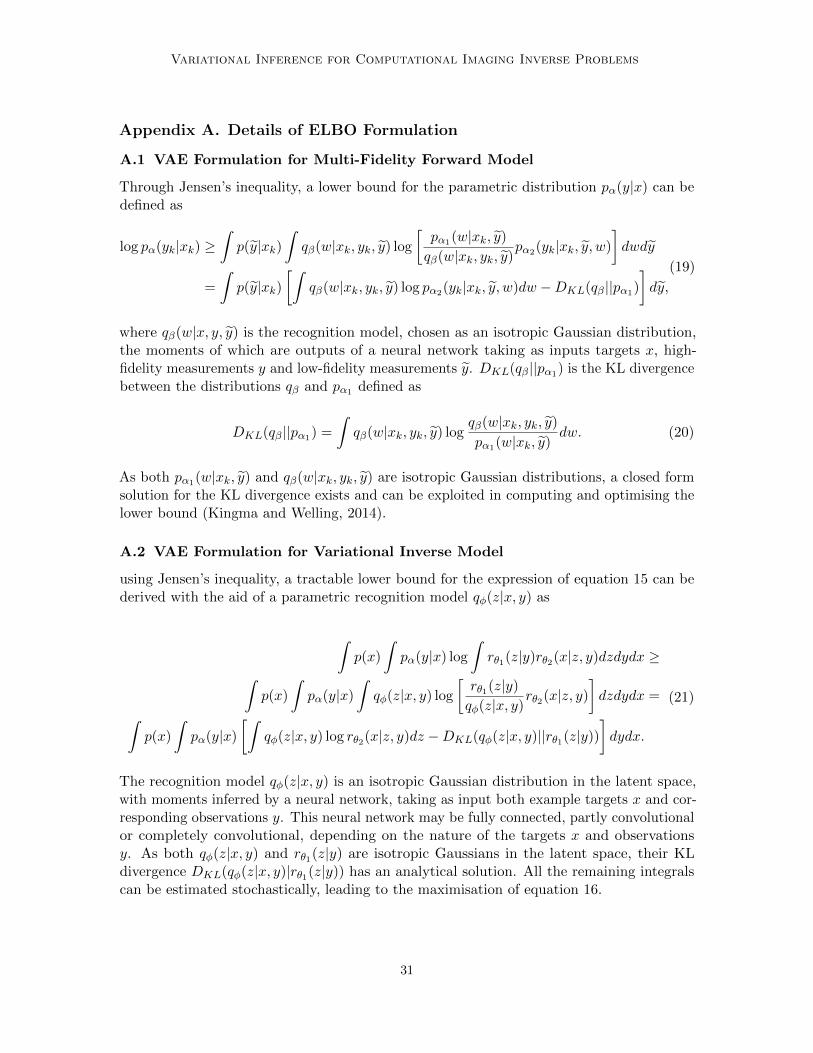
Variational Inference for Computational Imaging Inverse Problems
Appendix A. Details of ELBO Formulation
A.1 VAE Formulation for Multi-Fidelity Forward Model
Through Jensen’s inequality, a lower bound for the parametric distribution pα(y|x) can bedefined as
log pα(yk|xk) ≥∫p(y|xk)
∫qβ(w|xk, yk, y) log
[pα1(w|xk, y)
qβ(w|xk, yk, y)pα2(yk|xk, y, w)
]dwdy
=
∫p(y|xk)
[∫qβ(w|xk, yk, y) log pα2(yk|xk, y, w)dw −DKL(qβ||pα1)
]dy,
(19)
where qβ(w|x, y, y) is the recognition model, chosen as an isotropic Gaussian distribution,the moments of which are outputs of a neural network taking as inputs targets x, high-fidelity measurements y and low-fidelity measurements y. DKL(qβ||pα1) is the KL divergencebetween the distributions qβ and pα1 defined as
DKL(qβ||pα1) =
∫qβ(w|xk, yk, y) log
qβ(w|xk, yk, y)
pα1(w|xk, y)dw. (20)
As both pα1(w|xk, y) and qβ(w|xk, yk, y) are isotropic Gaussian distributions, a closed formsolution for the KL divergence exists and can be exploited in computing and optimising thelower bound (Kingma and Welling, 2014).
A.2 VAE Formulation for Variational Inverse Model
using Jensen’s inequality, a tractable lower bound for the expression of equation 15 can bederived with the aid of a parametric recognition model qφ(z|x, y) as
∫p(x)
∫pα(y|x) log
∫rθ1(z|y)rθ2(x|z, y)dzdydx ≥∫
p(x)
∫pα(y|x)
∫qφ(z|x, y) log
[rθ1(z|y)
qφ(z|x, y)rθ2(x|z, y)
]dzdydx =∫
p(x)
∫pα(y|x)
[∫qφ(z|x, y) log rθ2(x|z, y)dz −DKL(qφ(z|x, y)||rθ1(z|y))
]dydx.
(21)
The recognition model qφ(z|x, y) is an isotropic Gaussian distribution in the latent space,with moments inferred by a neural network, taking as input both example targets x and cor-responding observations y. This neural network may be fully connected, partly convolutionalor completely convolutional, depending on the nature of the targets x and observationsy. As both qφ(z|x, y) and rθ1(z|y) are isotropic Gaussians in the latent space, their KLdivergence DKL(qφ(z|x, y)|rθ1(z|y)) has an analytical solution. All the remaining integralscan be estimated stochastically, leading to the maximisation of equation 16.
31
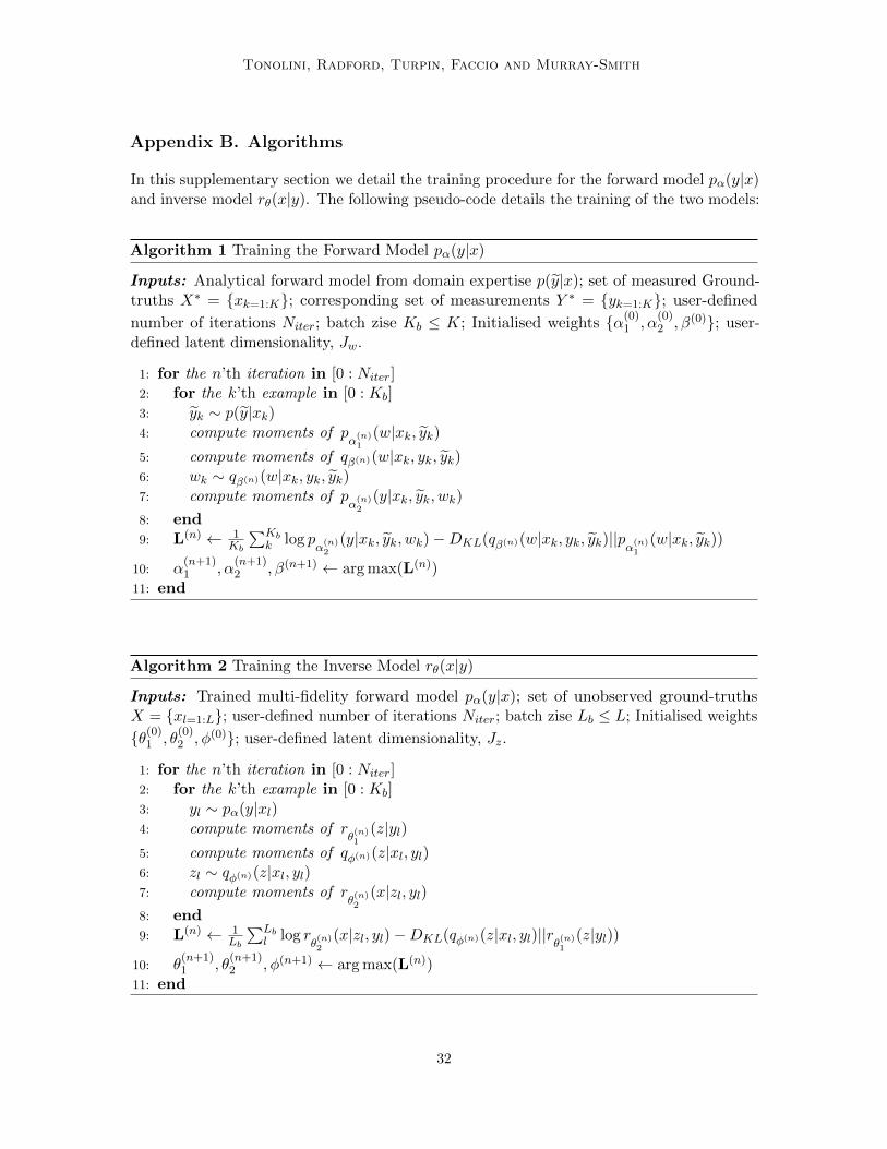
Tonolini, Radford, Turpin, Faccio and Murray-Smith
Appendix B. Algorithms
In this supplementary section we detail the training procedure for the forward model pα(y|x)and inverse model rθ(x|y). The following pseudo-code details the training of the two models:
Algorithm 1 Training the Forward Model pα(y|x)
Inputs: Analytical forward model from domain expertise p(y|x); set of measured Ground-truths X∗ = {xk=1:K}; corresponding set of measurements Y ∗ = {yk=1:K}; user-defined
number of iterations Niter; batch zise Kb ≤ K; Initialised weights {α(0)1 , α
(0)2 , β(0)}; user-
defined latent dimensionality, Jw.
1: for the n’th iteration in [0 : Niter]2: for the k’th example in [0 : Kb]3: yk ∼ p(y|xk)4: compute moments of p
α(n)1
(w|xk, yk)5: compute moments of qβ(n)(w|xk, yk, yk)6: wk ∼ qβ(n)(w|xk, yk, yk)7: compute moments of p
α(n)2
(y|xk, yk, wk)8: end9: L(n) ← 1
Kb
∑Kbk log p
α(n)2
(y|xk, yk, wk)−DKL(qβ(n)(w|xk, yk, yk)||pα(n)1
(w|xk, yk))
10: α(n+1)1 , α
(n+1)2 , β(n+1) ← arg max(L(n))
11: end
Algorithm 2 Training the Inverse Model rθ(x|y)
Inputs: Trained multi-fidelity forward model pα(y|x); set of unobserved ground-truthsX = {xl=1:L}; user-defined number of iterations Niter; batch zise Lb ≤ L; Initialised weights
{θ(0)1 , θ(0)2 , φ(0)}; user-defined latent dimensionality, Jz.
1: for the n’th iteration in [0 : Niter]2: for the k’th example in [0 : Kb]3: yl ∼ pα(y|xl)4: compute moments of r
θ(n)1
(z|yl)5: compute moments of qφ(n)(z|xl, yl)6: zl ∼ qφ(n)(z|xl, yl)7: compute moments of r
θ(n)2
(x|zl, yl)8: end9: L(n) ← 1
Lb
∑Lbl log r
θ(n)2
(x|zl, yl)−DKL(qφ(n)(z|xl, yl)||rθ(n)1
(z|yl))
10: θ(n+1)1 , θ
(n+1)2 , φ(n+1) ← arg max(L(n))
11: end
32
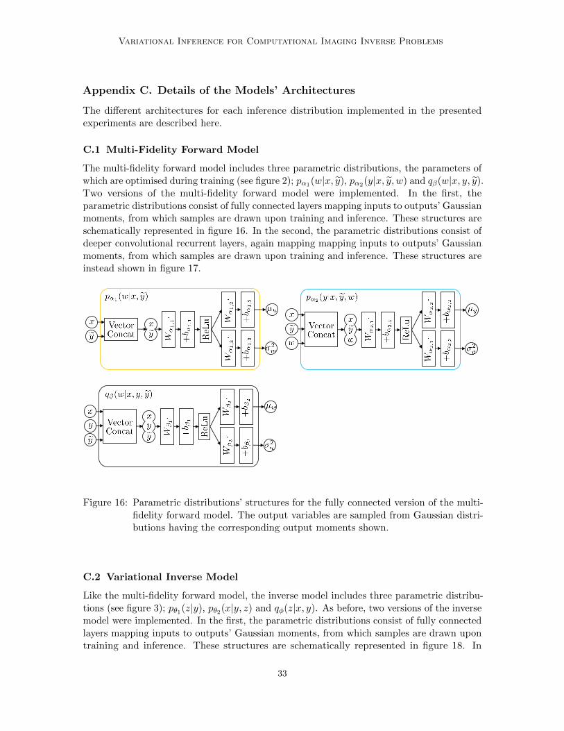
Variational Inference for Computational Imaging Inverse Problems
Appendix C. Details of the Models’ Architectures
The different architectures for each inference distribution implemented in the presentedexperiments are described here.
C.1 Multi-Fidelity Forward Model
The multi-fidelity forward model includes three parametric distributions, the parameters ofwhich are optimised during training (see figure 2); pα1(w|x, y), pα2(y|x, y, w) and qβ(w|x, y, y).Two versions of the multi-fidelity forward model were implemented. In the first, theparametric distributions consist of fully connected layers mapping inputs to outputs’ Gaussianmoments, from which samples are drawn upon training and inference. These structures areschematically represented in figure 16. In the second, the parametric distributions consist ofdeeper convolutional recurrent layers, again mapping mapping inputs to outputs’ Gaussianmoments, from which samples are drawn upon training and inference. These structures areinstead shown in figure 17.
1
Figure 16: Parametric distributions’ structures for the fully connected version of the multi-fidelity forward model. The output variables are sampled from Gaussian distri-butions having the corresponding output moments shown.
C.2 Variational Inverse Model
Like the multi-fidelity forward model, the inverse model includes three parametric distribu-tions (see figure 3); pθ1(z|y), pθ2(x|y, z) and qφ(z|x, y). As before, two versions of the inversemodel were implemented. In the first, the parametric distributions consist of fully connectedlayers mapping inputs to outputs’ Gaussian moments, from which samples are drawn upontraining and inference. These structures are schematically represented in figure 18. In
33
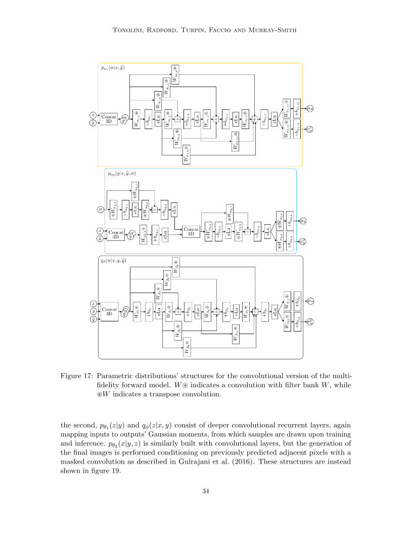
Tonolini, Radford, Turpin, Faccio and Murray-Smith
Figure 17: Parametric distributions’ structures for the convolutional version of the multi-fidelity forward model. W~ indicates a convolution with filter bank W , while~W indicates a transpose convolution.
the second, pθ1(z|y) and qφ(z|x, y) consist of deeper convolutional recurrent layers, againmapping inputs to outputs’ Gaussian moments, from which samples are drawn upon trainingand inference. pθ2(x|y, z) is similarly built with convolutional layers, but the generation ofthe final images is performed conditioning on previously predicted adjacent pixels with amasked convolution as described in Gulrajani et al. (2016). These structures are insteadshown in figure 19.
34
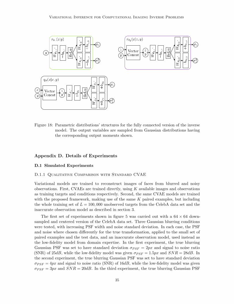
Variational Inference for Computational Imaging Inverse Problems
1
Figure 18: Parametric distributions’ structures for the fully connected version of the inversemodel. The output variables are sampled from Gaussian distributions havingthe corresponding output moments shown.
Appendix D. Details of Experiments
D.1 Simulated Experiments
D.1.1 Qualitative Comparison with Standard CVAE
Variational models are trained to reconstruct images of faces from blurred and noisyobservations. First, CVAEs are trained directly, using K available images and observationsas training targets and conditions respectively. Second, the same CVAE models are trainedwith the proposed framework, making use of the same K paired examples, but includingthe whole training set of L = 100, 000 unobserved targets from the CelebA data set and theinaccurate observation model as described in section 3.
The first set of experiments shown in figure 5 was carried out with a 64 × 64 down-sampled and centered version of the CelebA data set. Three Gaussian blurring conditionswere tested, with increasing PSF width and noise standard deviation. In each case, the PSFand noise where chosen differently for the true transformation, applied to the small set ofpaired examples and the test data, and an inaccurate observation model, used instead asthe low-fidelity model from domain expertise. In the first experiment, the true blurringGaussian PSF was set to have standard deviation σPSF = 2px and signal to noise ratio(SNR) of 25dB, while the low-fidelity model was given σPSF = 1.5px and SNR = 28dB. Inthe second experiment, the true blurring Gaussian PSF was set to have standard deviationσPSF = 4px and signal to noise ratio (SNR) of 16dB, while the low-fidelity model was givenσPSF = 3px and SNR = 20dB. In the third experiment, the true blurring Gaussian PSF
35
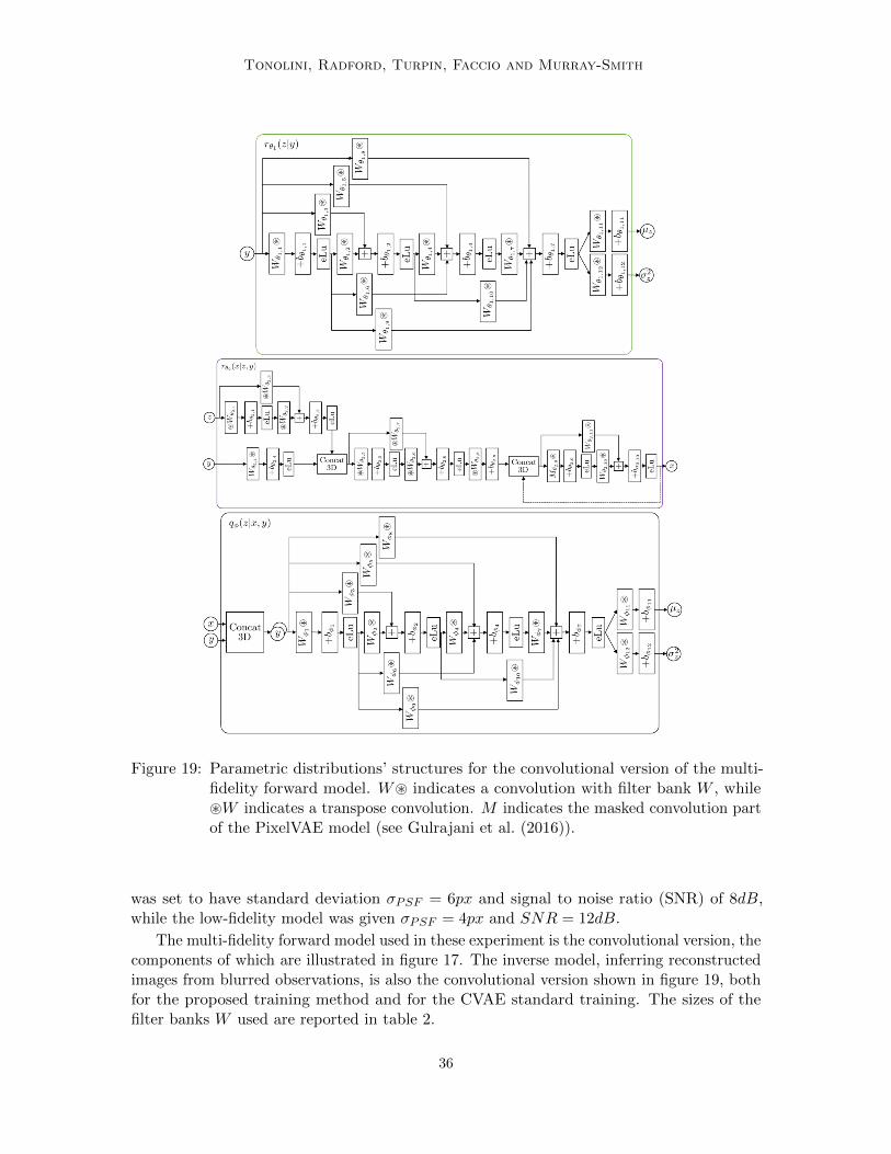
Tonolini, Radford, Turpin, Faccio and Murray-Smith
Figure 19: Parametric distributions’ structures for the convolutional version of the multi-fidelity forward model. W~ indicates a convolution with filter bank W , while~W indicates a transpose convolution. M indicates the masked convolution partof the PixelVAE model (see Gulrajani et al. (2016)).
was set to have standard deviation σPSF = 6px and signal to noise ratio (SNR) of 8dB,while the low-fidelity model was given σPSF = 4px and SNR = 12dB.
The multi-fidelity forward model used in these experiment is the convolutional version, thecomponents of which are illustrated in figure 17. The inverse model, inferring reconstructedimages from blurred observations, is also the convolutional version shown in figure 19, bothfor the proposed training method and for the CVAE standard training. The sizes of thefilter banks W used are reported in table 2.
36

Variational Inference for Computational Imaging Inverse Problems
Table 2: Filter banks of the multi-fidelity forward model and variational inverse model usedin the experiments of figure 5. The table reports the filter bank name used in thearchitectures shown in figures 17 and 19, filters height×width×number of channelsand strides of the convolutions.
Filters h × w × c Strides Filters h × w × c Strides
Wα1,1 12× 12× 10 2× 2 Wα1,2 12× 12× 10 1× 1
Wα1,3 12× 12× 10 2× 2 Wα1,4 12× 12× 10 2× 2
Wα1,5 12× 12× 10 4× 4 Wα1,6 12× 12× 10 2× 2
Wα1,7 12× 12× 10 2× 2 Wα1,8 12× 12× 10 8× 8
Wα1,9 12× 12× 10 2× 2 Wα1,10 12× 12× 10 4× 4
Wα1,11 12× 12× 3 1× 1 Wα1,12 12× 12× 3 1× 1
Wα2,1 12× 12× 10 2× 2 Wα2,2 12× 12× 10 2× 2
Wα2,3 12× 12× 10 4× 4 Wα2,4 12× 12× 10 2× 2
Wα2,5 12× 12× 10 1× 1 Wα2,6 12× 12× 10 2× 2
Wα2,7 12× 12× 10 2× 2 Wα2,8 12× 12× 3 1× 1
Wα2,9 12× 12× 3 1× 1
Wβ1 12× 12× 10 2× 2 Wβ2 12× 12× 10 1× 1
Wβ3 12× 12× 10 2× 2 Wβ4 12× 12× 10 2× 2
Wβ5 12× 12× 10 4× 4 Wβ6 12× 12× 10 2× 2
Wβ7 12× 12× 10 2× 2 Wβ8 12× 12× 10 8× 8
Wβ9 12× 12× 10 4× 4 Wβ10 12× 12× 10 2× 2
Wβ11 12× 12× 3 1× 1 Wβ12 12× 12× 3 1× 1
Wθ1,1 9× 9× 30 2× 2 Wθ1,2 9× 9× 30 1× 1
Wθ1,3 9× 9× 30 2× 2 Wθ1,4 9× 9× 30 2× 2
Wθ1,5 9× 9× 30 4× 4 Wθ1,6 9× 9× 30 2× 2
Wθ1,7 9× 9× 30 2× 2 Wθ1,8 9× 9× 30 8× 8
Wθ1,9 9× 9× 30 4× 4 Wθ1,10 9× 9× 30 2× 2
Wθ1,11 9× 9× 3 1× 1 Wθ1,12 9× 9× 3 1× 1
Wθ2,1 9× 9× 30 2× 2 Wθ2,2 9× 9× 30 2× 2
Wθ2,3 9× 9× 30 4× 4 Wθ2,4 9× 9× 30 2× 2
Wθ2,5 9× 9× 30 1× 1 Wθ2,6 9× 9× 30 2× 2
Wθ2,7 9× 9× 30 2× 2 Wθ2,8 9× 9× 3 1× 1
Mθ2,9 9× 9× 10 1× 1 Wθ2,10 9× 9× 3 1× 1
Wφ1 9× 9× 30 2× 2 Wφ2 9× 9× 30 1× 1
Wφ3 9× 9× 30 2× 2 Wφ4 9× 9× 30 2× 2
Wφ5 9× 9× 30 4× 4 Wφ6 9× 9× 30 2× 2
Wφ7 9× 9× 30 2× 2 Wφ8 9× 9× 30 8× 8
Wφ9 9× 9× 30 4× 4 Wφ10 9× 9× 30 2× 2
Wφ11 9× 9× 3 1× 1 Wφ12 9× 9× 3 1× 1
37
Tonolini, Radford, Turpin, Faccio and Murray-Smith
D.1.2 PSNR and ELBO versus Number of Examples
The set of experiments giving results shown in figure 6 is carried out on a 32 × 32 down-sampled version of the CelebA data set. Images are blurred with a Gaussian PSF havinga standard deviation of 2 pixels. As before, the standard CVAEs are trained with the Kimage-observation pairs alone. The proposed framework is then applied in each condition,exploiting the same K paired images and observations, L = 100, 000 unobserved targetexamples and an inaccurate observation model. Two different inaccurate observation modelsare used; a more accurate one with 10% under-estimation of PSF width and noise level and aless accurate one, having 40% under-estimation. After training each model, reconstructionsare performed with 2, 000 test examples and two quantitative measures are extracted: (i) theaverage peak signal to noise ration (PSNR) between the pseudo-maximum reconstructionsand the original images and (ii) the evidence lower bound (ELBO). The former serves as ameasure of deterministic performance, giving an index of similarity between the ground truthand the most likely reconstruction. The latter is a measure of probabilistic performance, as itapproximates the likelihood assigned by the model to the ground truths and consequentiallyis an index of how well the distribution of solutions to the inverse model is captured.
The forward multi-fidelity model used in the proposed methods is built with the simplefully connected structures of figure 16. The comparison CVAE and the inverse modelsare identical and are built with the fully connected structures of figure 18. Multi-fidelityforward models were built to have 300 hidden units in all deterministic layers, while thelatent variable w was chosen to be 100-dimensional. The inverse models, both for theproposed framework and the comparative CVAE, were built with 2500 hidden units in thedeterministic layers and latent variables z of 800 dimensions.
D.1.3 Qualitative Comparison with Alternative Training Strategies
The results of figure 7 were obtained by reconstructing from blurred 64× 64 CelebA images,blurred with a Gaussian PSF having standard deviation of 4 pixels and additive gaussiannoise, corresponding to a SNR of 16dB. The inaccurate observation model was instead givena PSF with standard deviation of 3 pixels and no additive noise.
The multi-fidelity forward model used in these experiments was of the convolutionalform shown in figure 17, with the filter structures reported in table 2.
D.1.4 Quantitative Comparison with Alternative Training Strategies
Four different degradation conditions where tested, applying the following four degradationsto 32× 32 CelebA and CIFAR10 images:
• × 2 Down-Sampling. The true transformation applied to the K observed imagesconsists of a ×2 down-sampling of the images in each dimension and a subsequentblurring with a PSF having standard deviation 1.4 pixels. The low-fidelity accessiblemodel down-samples by 2, but does not apply any blurring afterwards (i.e. the sourceof inaccuracy in the known forward model derives from ignoring blurring).
• Partial Occlusion. In the true transformation applied to the K observed images,a rectangular section of 8× 11 pixels is set to zero in a given position in all images.
38
Variational Inference for Computational Imaging Inverse Problems
The low-fidelity model places instead a 5× 15 at random with a difference in centralposition of dy = 2 and dx = −2.
• Gaussian Blurring, σPSF = 2.5px. The true transformation blurs the images witha PSF having standard deviation σPSF = 2.5 pixels and additive Gaussian noise at12dB. The low-fidelity analytical model instead blurs the images with a PSF havingstandard deviation σPSF = 1.5 pixels and does not add any noise.
• Gaussian Blurring, σPSF = 1.5px. The true transformation blurs the images witha PSF having standard deviation σPSF = 1.5 pixels and additive Gaussian noise at16dB. The low-fidelity analytical model instead blurs the images with a PSF havingstandard deviation σPSF = 1 pixels and does not add any noise.
The forward multi-fidelity model used in the proposed methods is built with the simplefully connected structures of figure 16. All inversion models, competitive and proposed,were implemented with the fully connected version of the inverse model given in figure 18.Multi-fidelity forward models were built to have 300 hidden units in all deterministic layers,while the latent variable w was chosen to be 100-dimensional. The inverse models, both forthe proposed framework and the comparative training methods, were built with 2500 hiddenunits in the deterministic layers and latent variables z of 800 dimensions.
D.2 Holographic Image Reconstruction
We provide here more details on the HIO algorithm. The HIO algorithm is a Fouriertransform-based method for holographic reconstruction where some constraints are used assupport. In our case we have access to the amplitude at the camera plane and we assumethat the phase at the DMD plane is uniform accross all micromirrors. The HIO algorithmstarts with a random guess of the phase of the recorded image at the camera, performs aninverse Fourier transform to obtain a guess of both amplitude and phase at the DMD plane,and replaces the obtained phase with a uniform phase (one of our constraints). At this point,further constraints are added e.g. there is only image information at the central N ×Mpixels of the image (with N,M being arbitrary). After that, a forward Fourier transformis performed and the corresponding amplitude is replaced by the image recorded by thecamera. This process is repeated iteratively. The problem is that if the recorded imageis saturated and down-sampled, the iterative process breaks after the first iteration. As aconsequence, it is impossible for the algorithm to converge towards a solution close to theground truth. This is precisely what we observe in Figure 10(c), where the HIO algorithmsimply predicts spots at some positions.
D.3 ToF Diffuse Imaging
The comparative iterative method was taken from Lyons et al. (2019), reproducing exactlythe main results therein. For the proposed variational method, only the first 15 framesof the recorded experimental video were used as observation, as most of the informationis contained in the rising front of the signal and around the peak. Consequentially, thecorresponding frames in the two simulations (high and low fidelity) were used to train themodel. The forward multi-fidelity model for the proposed variational method was built
39

Tonolini, Radford, Turpin, Faccio and Murray-Smith
with the fully connected structures shown in figure 16, with all deterministic intermediatelayers having 3000 hidden units and latent variables w having 100 dimensions. The inversemodel was also constructed using fully connected structures, as shown in figure 18, with alldeterministic intermediate layers having 1500 hidden units and latent variables z having 800dimensions.
40
Variational Inference for Computational Imaging Inverse Problems
References
Jonas Adler and Ozan Oktem. Solving ill-posed inverse problems using iterative deep neuralnetworks. Inverse Problems, 33(12):124007, 2017.
Jonas Adler and Ozan Oktem. Deep Bayesian inversion. arXiv preprint arXiv:1811.05910,2018.
Hemant K. Aggarwal, Merry P. Mani, and Mathews Jacob. MoDL: Model-based deeplearning architecture for inverse problems. IEEE Transactions on medical imaging, 38(2):394–405, 2019.
S. Derin Babacan, Rafael Molina, and Aggelos K. Katsaggelos. Variational Bayesian blinddeconvolution using a total variation prior. IEEE Transactions on Image Processing, 18(1):12–26, 2009.
S. Derin Babacan, Rafael Molina, and Aggelos K. Katsaggelos. Variational Bayesian superresolution. IEEE Transactions on Image Processing, 20(4):984–999, 2011.
David A. Barmherzig, Ju Sun, Po-Nan Li, Thomas Joseph Lane, and Emmanuel J. Candes.Holographic phase retrieval and reference design. Inverse Problems, 2019.
Maria J. Bayarri, James O. Berger, Rui Paulo, Jerry Sacks, John A. Cafeo, James Cavendish,Chin-Hsu Lin, and Jian Tu. A framework for validation of computer models. Technometrics,49(2):138–154, 2007.
Mario Bertero and Patrizia Boccacci. Introduction to inverse problems in imaging. CRCpress, 1998.
Jose M. Bioucas-Dias, Mario A.T. Figueiredo, and Joao Pedro Oliveira. Total variation-basedimage deconvolution: a majorization-minimization approach. In Acoustics, Speech andSignal Processing, 2006. ICASSP 2006 Proceedings. 2006 IEEE International Conferenceon, volume 2, pages II–II. IEEE, 2006.
Ashish Bora, Ajil Jalal, Eric Price, and Alexandros G. Dimakis. Compressed sensing usinggenerative models. Proceedings of the 34th International Conference on Machine Learning,PMLR, pages 537–546, 2017.
Emmanuel J. Candes, Justin K. Romberg, and Terence Tao. Stable signal recovery fromincomplete and inaccurate measurements. Communications on Pure and Applied Math-ematics: A Journal Issued by the Courant Institute of Mathematical Sciences, 59(8):1207–1223, 2006.
Stanley H. Chan, Xiran Wang, and Omar A. Elgendy. Plug-and-play ADMM for imagerestoration: Fixed-point convergence and applications. IEEE Transactions on Computa-tional Imaging, 3(1):84–98, 2017.
Jen-Hao Rick Chang, Chun-Liang Li, Barnabas Poczos, B. V. K. Vijaya Kumar, and Aswin C.Sankaranarayanan. One network to solve them all-solving linear inverse problems usingdeep projection models. In ICCV, pages 5889–5898, 2017.
41
Tonolini, Radford, Turpin, Faccio and Murray-Smith
Yunjin Chen, Wei Yu, and Thomas Pock. On learning optimized reaction diffusion processesfor effective image restoration. In Proceedings of the IEEE conference on computer visionand pattern recognition, pages 5261–5269, 2015.
J. Andres Christen and Colin Fox. Markov chain Monte Carlo using an approximation.Journal of Computational and Graphical statistics, 14(4):795–810, 2005.
Ingrid Daubechies, Michel Defrise, and Christine De Mol. An iterative thresholding algorithmfor linear inverse problems with a sparsity constraint. Communications on Pure andApplied Mathematics: A Journal Issued by the Courant Institute of Mathematical Sciences,57(11):1413–1457, 2004.
David L. Donoho. Compressed sensing. IEEE Transactions on information theory, 52(4):1289–1306, 2006.
Michael Egmont-Petersen, Dick de Ridder, and Heinz Handels. Image processing with neuralnetworks – a review. Pattern recognition, 35(10):2279–2301, 2002.
Helen Mary Louise Faulkner and J.M. Rodenburg. Movable aperture lensless transmissionmicroscopy: a novel phase retrieval algorithm. Physical review letters, 93(2):023903, 2004.
James R. Fienup. Phase retrieval algorithms: a comparison. Applied optics, 21(15):2758–2769,1982.
Mario A.T. Figueiredo, Robert D. Nowak, and Stephen J. Wright. Gradient projectionfor sparse reconstruction: Application to compressed sensing and other inverse problems.IEEE Journal of selected topics in signal processing, 1(4):586–597, 2007.
Dani Gamerman and Hedibert F. Lopes. Markov chain Monte Carlo: stochastic simulationfor Bayesian inference. Chapman and Hall/CRC, 2006.
Ralph W. Gerchberg. A practical algorithm for the determination of phase from image anddiffraction plane pictures. Optik, 35:237–246, 1972.
Ishaan Gulrajani, Kundan Kumar, Faruk Ahmed, Adrien Ali Taiga, Francesco Visin, DavidVazquez, and Aaron Courville. PixelVAE: A latent variable model for natural images.arXiv preprint arXiv:1611.05013, 2016.
Paul Hand, Oscar Leong, and Vlad Voroninski. Phase retrieval under a generative prior. InAdvances in Neural Information Processing Systems, pages 9154–9164, 2018.
Phillip Isola, Jun-Yan Zhu, Tinghui Zhou, and Alexei A. Efros. Image-to-image translationwith conditional adversarial networks. In Proceedings of the IEEE conference on computervision and pattern recognition, pages 1125–1134, 2017.
Alexander Jesacher, Christian Maurer, Andreas Schwaighofer, Stefan Bernet, and MonikaRitsch-Marte. Full phase and amplitude control of holographic optical tweezers with highefficiency. Optics express, 16(7):4479–4486, 2008.
Shihao Ji, Ya Xue, and Lawrence Carin. Bayesian compressive sensing. IEEE Transactionson Signal Processing, 56(6):2346, 2008.
42
Variational Inference for Computational Imaging Inverse Problems
Huabei Jiang. Diffuse optical tomography: principles and applications. CRC press, 2018.
Sherena G. Johnson. NIST Special Database 30. 2010.
Jari Kaipio and Erkki Somersalo. Statistical inverse problems: discretization, model reductionand inverse crimes. Journal of computational and applied mathematics, 198(2):493–504,2007.
Marc C. Kennedy and Anthony O’Hagan. Bayesian calibration of computer models. Journalof the Royal Statistical Society: Series B (Statistical Methodology), 63(3):425–464, 2001.
D. P. Kingma and M. Welling. Auto-encoding variational Bayes. Proceedings of the 2ndInternational Conference on Learning Representations (ICLR), 2014.
Durk P. Kingma, Shakir Mohamed, Danilo Jimenez Rezende, and Max Welling. Semi-supervised learning with deep generative models. In Advances in neural informationprocessing systems, pages 3581–3589, 2014.
Alex Krizhevsky. Learning multiple layers of features from tiny images. Master’s thesis,University of Toronto, 2009.
Kuldeep Kulkarni, Suhas Lohit, Pavan Turaga, Ronan Kerviche, and Amit Ashok. Reconnet:Non-iterative reconstruction of images from compressively sensed measurements. InProceedings of the IEEE Conference on Computer Vision and Pattern Recognition, pages449–458, 2016.
Christian Ledig, Lucas Theis, Ferenc Huszar, Jose Caballero, Andrew Cunningham, AlejandroAcosta, Andrew P. Aitken, Alykhan Tejani, Johannes Totz, Zehan Wang, and Wenzhe Shi.Photo-realistic single image super-resolution using a generative adversarial network. InIEEE Conference on Computer Vision and Pattern Recognition (CVPR), pages 105–114,2017.
June-Goo Lee, Sanghoon Jun, Young-Won Cho, Hyunna Lee, Guk Bae Kim, Joon BeomSeo, and Namkug Kim. Deep learning in medical imaging: general overview. KoreanJournal of Radiology, 18(4):570–584, 2017.
Aristidis Likas and Nikolas P. Galatsanos. A variational approach for Bayesian blind imagedeconvolution. IEEE Transactions on Signal Processing, 52(8):2222–2233, 2004.
Ziwei Liu, Ping Luo, Xiaogang Wang, and Xiaoou Tang. Deep learning face attributes inthe wild. In Proceedings of International Conference on Computer Vision (ICCV), 2015.
Alice Lucas, Michael Iliadis, Rafael Molina, and Aggelos K Katsaggelos. Using deep neuralnetworks for inverse problems in imaging: beyond analytical methods. IEEE SignalProcessing Magazine, 35(1):20–36, 2018.
Ashley Lyons, Francesco Tonolini, Alessandro Boccolini, Audrey Repetti, Robert Henderson,Yves Wiaux, and Daniele Faccio. Computational time-of-flight diffuse optical tomography.Nature Photonics, 13:575–579, 2019.
43
Tonolini, Radford, Turpin, Faccio and Murray-Smith
Lars Maaløe, Casper Kaae Sønderby, Søren Kaae Sønderby, and Ole Winther. Auxiliarydeep generative models. In Proceedings of the 33rd International Conference on MachineLearning (ICML), 2016.
Filipe Magalhaes, Francisco M. Araujo, Miguel V. Correia, Mehrdad Abolbashari, andFaramarz Farahi. Active illumination single-pixel camera based on compressive sensing.Applied optics, 50(4):405–414, 2011.
Alberto Malinverno. Parsimonious Bayesian Markov chain Monte Carlo inversion in anonlinear geophysical problem. Geophysical Journal International, 151(3):675–688, 2002.
S Marchesini, H.N. Chapman, S.P. Hau-Riege, R.A. London, A. Szoke, H. He, M.R. Howells,H. Padmore, R. Rosen, J.C.H. Spence, and U. Weierstall. Coherent X-ray diffractiveimaging: applications and limitations. Optics Express, 11(19):2344–2353, 2003.
M. Mardani, E. Gong, J. Y. Cheng, S. S. Vasanawala, G. Zaharchuk, L. Xing, and J. M.Pauly. Deep generative adversarial networks for compressed sensing automates MRI.IEEE Transactions on Medical Imaging, 32(1):167–179, Jan 2019.
James Martin, Lucas C Wilcox, Carsten Burstedde, and Omar Ghattas. A stochastic NewtonMCMC method for large-scale statistical inverse problems with application to seismicinversion. SIAM Journal on Scientific Computing, 34(3):A1460–A1487, 2012.
Youssef Marzouk and Dongbin Xiu. A stochastic collocation approach to Bayesian inferencein inverse problems. Communications in Computational Physics, 6(4):826–847, 2009.
Kiyotoshi Matsuoka. Noise injection into inputs in back-propagation learning. IEEETransactions on Systems, Man, and Cybernetics, 22(3):436–440, 1992.
Michael T. McCann, Kyong Hwan Jin, and Michael Unser. A review of convolutional neuralnetworks for inverse problems in imaging. IEEE Signal Processing Magazine, 34(6):85–95,November 2017.
Mehdi Mirza and Simon Osindero. Conditional generative adversarial nets. arXiv preprintarXiv:1411.1784, 2014.
Ali Mohammad-Djafari. Bayesian inference tools for inverse problems. In AIP ConferenceProceedings, volume 1553, pages 163–170. AIP, 2013.
Eric Nalisnick, Akihiro Matsukawa, Yee Whye Teh, Dilan Gorur, and Balaji Lakshmi-narayanan. Hybrid models with deep and invertible features. In Proc. 36th InternationalConference on Machine Learning (ICML), Long Beach, California, PMLR 97., 2019.
Alfredo Nazabal, Pablo M. Olmos, Zoubin Ghahramani, and Isabel Valera. Handlingincomplete heterogeneous data using VAEs. Pattern Recognition, 107501, 107, Nov .
Anh Nguyen, Jeff Clune, Yoshua Bengio, Alexey Dosovitskiy, and Jason Yosinski. Plug &play generative networks: Conditional iterative generation of images in latent space. InCVPR, volume 2, page 7, 2017.
44
Variational Inference for Computational Imaging Inverse Problems
Augustus Odena, Christopher Olah, and Jonathon Shlens. Conditional image synthesis withauxiliary classifier GANs. In Proceedings of the 34th International Conference on MachineLearnin (ICML), PMLR 70, pages 2642–2651, 2017.
Stanley Osher, Martin Burger, Donald Goldfarb, Jinjun Xu, and Wotao Yin. An iterativeregularization method for total variation-based image restoration. Multiscale Modeling &Simulation, 4(2):460–489, 2005.
Niki Parmar, Ashish Vaswani, Jakob Uszkoreit, Lukasz Kaiser, Noam Shazeer, Alexander Ku,and Dustin Tran. Image transformer. Proceedings of the 35th International Conference onMachine Learning, Stockholm, Sweden, PMLR 80, 2018.
Deepak Pathak, Philipp Krahenbuhl, Jeff Donahue, Trevor Darrell, and Alexei A. Efros.Context encoders: Feature learning by inpainting. In Proceedings of the IEEE conferenceon computer vision and pattern recognition, pages 2536–2544, 2016.
Benjamin Peherstorfer, Karen Willcox, and Max Gunzburger. Survey of multifidelity methodsin uncertainty propagation, inference, and optimization. SIAM Review, 60(3):550–591,2018.
Patrick Putzky and Max Welling. Recurrent inference machines for solving inverse problems.arXiv preprint arXiv:1706.04008, 2017.
Scott Reed, Zeynep Akata, Xinchen Yan, Lajanugen Logeswaran, Bernt Schiele, and HonglakLee. Generative adversarial text to image synthesis. Proceedings of the 33rd InternationalConference on Machine Learning, 2016.
Ludwig Ritschl, Frank Bergner, Christof Fleischmann, and Marc Kachelrieß. Improved totalvariation-based CT image reconstruction applied to clinical data. Physics in Medicine &Biology, 56(6):1545, 2011.
Yair Rivenson, Yibo Zhang, Harun Gunaydın, Da Teng, and Aydogan Ozcan. Phase recoveryand holographic image reconstruction using deep learning in neural networks. Light:Science & Applications, 7(2):17141, 2018.
Yair Rivenson, Yichen Wu, and Aydogan Ozcan. Deep learning in holography and coherentimaging. Light: Science & Applications, 8(1):1–8, 2019.
Yoav Shechtman, Yonina C. Eldar, Oren Cohen, Henry Nicholas Chapman, Jianwei Miao,and Mordechai Segev. Phase retrieval with application to optical imaging: a contemporaryoverview. IEEE signal processing magazine, 32(3):87–109, 2015.
Ayan Sinha, Justin Lee, Shuai Li, and George Barbastathis. Lensless computational imagingthrough deep learning. Optica, 4(9):1117–1125, 2017.
Kihyuk Sohn, Honglak Lee, and Xinchen Yan. Learning structured output representationusing deep conditional generative models. In Advances in Neural Information ProcessingSystems, pages 3483–3491, 2015.
45
Tonolini, Radford, Turpin, Faccio and Murray-Smith
Jean-Luc Starck, Mai K. Nguyen, and Fionn Murtagh. Wavelets and curvelets for imagedeconvolution: a combined approach. Signal processing, 83(10):2279–2283, 2003.
Baoqing Sun, Matthew P. Edgar, Richard Bowman, Liberty E. Vittert, Stuart Welsh, AdrianBowman, and Miles J. Padgett. 3D computational imaging with single-pixel detectors.Science, 340(6134):844–847, 2013.
Panagiotis Tsilifis, Ilias Bilionis, Ioannis Katsounaros, and Nicholas Zabaras. Computa-tionally efficient variational approximations for Bayesian inverse problems. Journal ofVerification, Validation and Uncertainty Quantification, 1(3):031004, 2016.
Andreas Velten, Thomas Willwacher, Otkrist Gupta, Ashok Veeraraghavan, Moungi G.Bawendi, and Ramesh Raskar. Recovering three-dimensional shape around a corner usingultrafast time-of-flight imaging. Nature communications, 3:745, 2012.
Curtis R. Vogel. Computational methods for inverse problems, volume 23. SIAM, 2002.
Li Xu, Jimmy S.J. Ren, Ce Liu, and Jiaya Jia. Deep convolutional neural network for imagedeconvolution. In Advances in Neural Information Processing Systems, pages 1790–1798,2014.
Xinchen Yan, Jimei Yang, Kihyuk Sohn, and Honglak Lee. Attribute2image: Conditionalimage generation from visual attributes. In European Conference on Computer Vision,pages 776–791. Springer, 2016.
Junfeng Yang and Yin Zhang. Alternating direction algorithms for `1-problems in compressivesensing. SIAM journal on scientific computing, 33(1):250–278, 2011.
Yibo Yang and Paris Perdikaris. Conditional deep surrogate models for stochastic, high-dimensional, and multi-fidelity systems. Computational Mechanics, 64:417–434, 2019.
K.M. Yoo, Feng Liu, and R.R. Alfano. When does the diffusion approximation fail todescribe photon transport in random media? Physical review letters, 64(22):2647, 1990.
Chen Zhang and Bangti Jin. Probabilistic residual learning for aleatoric uncertainty inimage restoration. arXiv preprint arXiv:1908.01010, 2019.
Cheng Zhang, Judith Butepage, Hedvig Kjellstrom, and Stephan Mandt. Advances invariational inference. IEEE transactions on pattern analysis and machine intelligence,2018.
Kai Zhang, Wangmeng Zuo, Shuhang Gu, and Lei Zhang. Learning deep CNN denoiserprior for image restoration. In Proceedings of the IEEE Conference on Computer Visionand Pattern Recognition, pages 3929–3938, 2017.
46