DISSERTATION

TROPICAL CYCLONE INNER CORE STRUCTURE AND INTENSITY CHANGE

Submitted by

Kate D. Musgrave

Department of Atmospheric Science

In partial fulfillment of the requirements

For the Degree of Doctor of Philosophy

Colorado State University

Fort Collins, Colorado

Fall 2011

Doctoral Committee:

Advisor: Wayne Schubert Co-Advisor: Christopher Davis

Richard Johnson David Thompson Michael Kirby

Copyright by Kate Dollen Musgrave 2011

All Rights Reserved

ABSTRACT

TROPICAL CYCLONE INNER CORE STRUCTURE AND INTENSITY CHANGE

This dissertation focuses on two projects that examine aspects of the relationship

between tropical cyclone (TC) storm-scale dynamics and intensity. TC intensity change

is a forecast challenge combining influences from the large-scale environment, the

underlying ocean state, and the storm-scale dynamics within the TC. In particular

structures and processes involving the TC eye are observed to have an impact on current

and future intensity.

The first project examines observations of TC eyes from aircraft reconnaissance

flown into Atlantic basin TCs over the period 1989-2008. Relationships between TC eye

diameter and type and intensity and intensity change are investigated. Consistent with

previous studies, eye diameter does not display a direct relationship with intensity.

Smaller eye diameters are observed at all intensities, though both the most and least

intense TCs with eyes have smaller average eye diameters. Smaller eyes also have the

largest variability in intensity change. Larger eyes show smaller ranges for intensity

change, and the largest eyes tend to maintain or weaken in intensity. TCs with eyes

reported had higher intensification rates and higher probabilities of undergoing rapid

intensification.

ii

iii

The second project takes a theoretical approach to examining the TC response to

the location of the convection within the vortex structure using the balanced vortex

model. An annular ring of heating is placed along an idealized axisymmetric vortex. The

largest increase in intensity is produced when the heating is placed within the radius of

maximum winds. Intensification still occurs at a lessened rate when the heating is

contained within the vorticity skirt, and when the heating is outside the vorticity skirt the

vortex does not intensify. The strength of the vortex increases in all cases, though less so

than the intensity when the heating is within the radius of maximum winds.

ACKNOWLEDGEMENTS

I would like to thank my advisor and co-advisor, Dr. Wayne Schubert and Dr.

Christopher Davis. They have worked with me through many transitions on the path to

completing this dissertation. Both CMMAP and SOARS provided invaluable support

during this process. My group members and the larger tropical cyclone group here at

CSU have contributed many useful discussions, particularly Jonathan Vigh, Brian

McNoldy, Rick Taft, John Knaff, Mark DeMaria, and Kate Maclay.

This dissertation would be incomplete without mentioning the support my family

and friends provided through this process, and expressing my gratitude to my husband

Chris Musgrave for his seemingly infinite patience over the years.

This material is based upon work supported by the National Science Foundation

under Grant ATM-0837932 and under the Science and Technology Center for Multi-

Scale Modeling of Atmospheric Processes, managed by Colorado State University

through cooperative agreement No. ATM-0425247. Additional support has been

provided by the National Oceanographic Partnership Program through ONR contract

N00014-10-1-0145.

iv

TABLE OF CONTENTS

1 Introduction 1.1 Overview . . . . . . . . . . . . . . . . . . . . . . . . . . . . . . . . . . . 1.2 TC Prediction . . . . . . . . . . . . . . . . . . . . . . . . . . . . . . . . . 1.3 Links between TC Structure and Intensity . . . . . . . . . . . . . . . . . . 1.3.1 Eye Contraction/Expansion . . . . . . . . . . . . . . . . . . . . . . . . . 1.3.2 Concentric Eyewall Cycles . . . . . . . . . . . . . . . . . . . . . . . . . 1.3.3 Annular Hurricanes . . . . . . . . . . . . . . . . . . . . . . . . . . . . . 1.3.4 Pinhole Eyes . . . . . . . . . . . . . . . . . . . . . . . . . . . . . . . . . 1.4 Structure of Dissertation . . . . . . . . . . . . . . . . . . . . . . . . . . . 2 Aircraft Reconnaissance Measurements of Atlantic Tropical Cyclone Eyes 2.1 Overview . . . . . . . . . . . . . . . . . . . . . . . . . . . . . . . . . . . 2.2 Introduction . . . . . . . . . . . . . . . . . . . . . . . . . . . . . . . . . . 2.3 Data . . . . . . . . . . . . . . . . . . . . . . . . . . . . . . . . . . . . . . 2.4 Results . . . . . . . . . . . . . . . . . . . . . . . . . . . . . . . . . . . . . 2.5 Discussion . . . . . . . . . . . . . . . . . . . . . . . . . . . . . . . . . . . 3 Effects of Vortex Structure on the Diabatically-Induced Intensification of Tropical Cyclones 3.1 Overview . . . . . . . . . . . . . . . . . . . . . . . . . . . . . . . . . . . 3.2 Introduction . . . . . . . . . . . . . . . . . . . . . . . . . . . . . . . . . . 3.2.1 Background . . . . . . . . . . . . . . . . . . . . . . . . . . . . . . . . . 3.2.2 Chapter Overview . . . . . . . . . . . . . . . . . . . . . . . . . . . . . . 3.3 Balanced Vortex Model . . . . . . . . . . . . . . . . . . . . . . . . . . . . 3.3.1 Diabatic Heating . . . . . . . . . . . . . . . . . . . . . . . . . . . . . . 3.3.2 Vortex Profile . . . . . . . . . . . . . . . . . . . . . . . . . . . . . . . . 3.3.3 Integrated Kinetic Energy . . . . . . . . . . . . . . . . . . . . . . . . . 3.4 Changes in Vortex Structure . . . . . . . . . . . . . . . . . . . . . . . . . 3.4.1 Vortex Response: Strength and Intensity . . . . . . . . . . . . . . . . . . 3.5 Summary . . . . . . . . . . . . . . . . . . . . . . . . . . . . . . . . . . . 4 Summary 4.1 Discussion . . . . . . . . . . . . . . . . . . . . . . . . . . . . . . . . . . . References

1 1 1 3 6 7 8 9

10

17 17 18 20 21 32

55

55 56 56 61 61 69 70 71 72 76 76

101 101

111

v

Chapter 1

INTRODUCTION

1.1 Overview

This dissertation focuses on the relationships found between tropical cyclone (TC)

structure and intensity – in particular between the TC eye and intensity trends. As such,

this chapter explains the background that influenced this choice of focus. The next

sections give an overview of TC forecasting and previous research into particular

observed TC structures that are believed to influence intensity. Following that is a more

detailed discussion of the structure of this dissertation, including information on the

particular research projects presented in Chapters 2 and 3.

1.2 TC Prediction

TCs, referred to as hurricanes, typhoons, and cyclones in various parts of the

globe, are responsible for extensive damage and loss of life. In the continental United

States alone, TC-related damage averages $10-11 billion dollars annually (in 2007

dollars, AMS Council 2007). These damages are expected to grow over time, due to

societal changes in vulnerable coastal regions. Attempts to minimize loss of life and

damage to property has led many governments to issue TC forecasts, so citizens can

better prepare for these systems. These forecasts are constantly being improved upon

through changes in available tools and better understanding of TC dynamics.

1

Three particular areas emerge when discussing TC forecasts: track, intensity, and

structure. Currently the National Hurricane Center (NHC) forecasts track and intensity

out to 120 hours, and wind radii out to 72 hours for the 34 kt and 50 kt wind speed

thresholds, and 36 hours for the 64 kt wind speed threshold. Each type of forecast adds

important information for public preparedness: track provides details for location and

timing, intensity provides details for severity, and structure provides additional details for

the areas addressed by both track and intensity.

TC track forecasts have shown significant improvements over the past decades.

Franklin et al. (2003) examined Atlantic track forecasts over the period 1970-2001 and

found annual percentage improvements of 1.3-2%, with greater improvements at longer

lead times. These numbers are similar to those found in McAdie and Lawrence (2000).

As can be seen in Figure 1.1, the longer-term improvements in TC track forecasts are also

reflected in the error (Figure 1.1(a)) and skill (Figure 1.1(b)) trends over the years 1990-

2008.

In contrast, TC intensity forecasts have seen little improvement through the past

few decades, as shown in Figure 1.2 for the period 1990-2008. This relative lack of

improvement is at least partially attributed to periods of rapid intensification, which can

result in very large errors in intensity forecasts (Kaplan and DeMaria 2003, Kaplan et al.

2010). NHC has designated intensity forecasting in general, and rapid intensity change

forecasts in particular, as top priorities for TC research (Rappaport et al. 2009).

Forecasts of TC structure are even more problematic than intensity, as a lack of

observations leads to difficulties analyzing and forecasting the low-level wind field.

While NHC has operationally forecast wind radii at 34, 50, and 64 kt for several years,

2

post-storm estimates of these radii were only introduced in 2004 and these estimates are

much less certain than post-storm estimates of intensity. The lack of certainty in the

analysis of the wind field renders attempts to verify forecasts of wind radii a questionable

endeavor, and verifications of wind radii are not displayed along with track and intensity

in Franklin (2009).

The differences between the improvements in TC track and intensity forecasts

help highlight fundamental differences in the prediction of these measures. TC track is to

first order dependent on the large-scale environment. TC intensity is dependent on the

large scale environment, the storm-scale dynamics, and the underlying ocean state

(Kaplan et al. 2010). This makes forecasting TC intensity a very complex and

interrelated problem, which is not yet fully understood.

1.3 Links between TC Structure and Intensity

While intensity is referred to separately from structure throughout this

dissertation, it is merely one metric of structure. Merrill (1984) defined multiple aspects

of structure, all of which can affect the destructiveness of a TC: intensity, size and

strength. Intensity is usually measured by the maximum sustained surface wind (MSW)

or the minimum sea-level pressure (MSLP) of the TC, and represents the extremes in TC

circulation. Size generally refers to the area of a TC’s circulation, which can be

measured through the radius of gale-force winds (17 ms-1, 34 kt) or the radius of the

outermost closed isobar (ROCI). Strength is defined as the average wind speed in the TC

circulation, and is often measured in terms of an average or integrated kinetic energy

(KE) over specified radii.

3

Changes in intensity, size, and strength can all be viewed in a simple plot of

tangential wind speed, as shown in Figure 1.3. Intensification refers to an increase in

intensity, either through an increase in the MSW or a decrease in MSLP. When

measured through pressure, intensification can also be called deepening. A decrease in

intensity is called weakening (not a decrease in strength). Growth refers to an expansion

in size, while strengthening is an increase in strength. Strength includes aspects of both

intensity and size, but can change while both other measures remain constant. While

intensity and changes of intensity are the most commonly used measures of structure,

they are often referred to separately from other measures of structure to emphasize the

effects that changes in a TC’s overall structure can have on the intensity metric.

The severity of a TC is generally communicated to the public through the

intensity, categorized in the Atlantic basin through the Saffir-Simpson hurricane scale

(Simpson and Riehl 1981, Simpson and Saffir 2007). This scale rates hurricanes (TCs

with MSW of at least 64 kt) into five categories based off of the damage that might be

anticipated (see Table 1.1). Category 3-5 hurricanes are considered “major” hurricanes.

The original version was designed to use MSLP to estimate both winds and storm surge,

but in use it is based off of the MSW. As such there is currently disagreement on the

representativeness of the Saffir-Simpson scale for the total damage potential of a TC.

Several researchers are working on ways to incorporate measures of both strength and

intensity to better describe the damage potential of a TC (Maclay et al. 2008, Powell and

Reinhold 2007, Kantha 2006).

Several studies have examined the distribution of various size and strength

measures in TCs and their relationships with intensity (Merrill 1984, Frank 1977,

4

Weatherford and Gray 1988a,b, Cocks and Gray 2002, Croxford and Barnes 2002,

Kimball and Mulekar 2004, Maclay et al. 2008, Dean et al. 2009). Very little direct

relationship is found between TC size and intensity. Merrill (1984) discusses size based

on ROCI, and finds that it is weakly correlated with intensity. However, he relates both

to lifecycle, based on idealized stages presented in Dunn and Miller (1960) and Riehl

(1979). Frank (1977) found that a storm’s size, as measured by the radius at which the

perturbation winds associated with the TC vanish, is relatively constant throughout the

TC’s lifetime. Dean et al. (2009) suggest that TC size is a function of the precursor

disturbance, not the large-scale environment. Cocks and Gray (2002) also found that the

size of a mature TC tended to be determined by the size of the TC at formation, based off

the radius of 15 ms-1 winds.

Studies examining TC strength produce a wider variety of results, depending on

the measures used to define strength. Weatherford and Gray (1988a) split TCs into two

regions, the inner core and outer core. The inner core was defined as the area within 1°

of the TC center, or 0-111 km radius. The outer core contained the area within 1-2.5° of

the TC center, or 111-278 km radius. The outer core strength, or the average wind speed

in the outer core, was found to have little relationship to intensity. Croxford and Barnes

(2002) found a much stronger correlation between strength and intensity, but made use of

a measure of inner core strength (where inner core is altered to the area 65-140 km in

radius). Ooyama (1969) examined strength based on a variety of outer radii, and found

the behavior of an idealized TC’s strength over its lifecycle to vary based on the outer

radii chosen for the examination. Strength measured to larger radii tended to continue

increasing over the entire lifecycle of the TC, while the strength calculated from smaller

5

radii more closely resembled the trends in the intensity. In general as the area over which

TC strength is calculated moves closer to the TC center, the better correlated strength and

intensity become.

Maclay et al. (2008) used a kinetic energy-based measure of strength over the

radii 0-200 km to establish a relationship between changes in strength and intensity.

They found that TCs generally intensify without strengthening, or strengthen and

weaken/maintain intensity. This is consistent with previous studies examining both size

and strength. They discuss two different types of strengthening processes, one due to the

large scale environmental forcing and the other due to storm-scale dynamics.

When discussing storm-scale dynamics, several TC structures have been observed

to influence intensity. In particular, several structures and processes involving the TC

eye have been observed to lead to distinct intensities and intensity trends. Knowledge of

the existence and size of a TC eye has also been determined to improve the variance in

the relationship between size and intensity (Weatherford and Gray 1988b). Several of

these structures and processes that focus on TC eyes are discussed below, including eye

contraction, concentric eyewall cycles, annular hurricanes, and pinhole eyes. Better

understanding of these structures and their links to intensity can assist in understanding

the dynamics of TCs and their prediction.

1.3.1 Eye Contraction/Expansion

It has long been known that while the size of a TC eye is not well correlated to

intensity, the change in the size of the eye can give useful information about the intensity

trend (Jordan 1961). Jordan (1961) noted that eye size tends to decrease in the 24 hour

period preceding maximum intensity (as measured by MSLP), and increase in the 24

6

hours after maximum intensity. This is in agreement with theoretical studies that suggest

that the smallest eye size should correspond with maximum intensity (Kuo 1959).

Shapiro and Willoughby (1982) explain the connection between eyewall

contraction and intensification through the context of a balanced vortex model (Eliassen

1952). Point sources of heat and momentum added near the radius of maximum winds

(RMW) lead to a contraction and intensification of the maximum winds. This result held

for sources of heat located both at and outside of the RMW, although once the source was

located at twice the radius of maximum winds it tended to expand the RMW, and either

maintain or decrease the intensity of the vortex.

1.3.2 Concentric Eyewall Cycles

Many TCs have been observed to form concentric eyewalls, with up to 70% of the

TCs in the Atlantic basin that reach intensities of 120 kt or more developing concentric

eyewalls (Hawkins et al. 2006). In these cases, an outer ring of convection forms around

the current (or inner) eyewall, with a “moat” or lack of convection between the rings.

Once the outer eyewall forms, it contracts and strengthens, while the inner eyewall

weakens and eventually disappears, as shown in Figure 1.4. These concentric eyewall

cycles also display characteristic changes in intensity. As the inner eyewall decays, the

TC tends to weaken in intensity, then as the outer eyewall contracts it tends to reintensify

the TC. Concentric eyewall cycles also have the potential to modify the strength of a TC

(Elsberry and Stenger 2008).

Numerous studies have explored concentric eyewall cycles from observational

(Jordan and Schlatzle 1961, Black and Willoughby 1992, McNoldy 2004, Hawkins et al.

2006, Houze et al. 2007, Kossin and Sitkowski 2009), theoretical (Willoughby et al.

7

1982, Kossin et al. 2000, Kuo et al. 2004, Kuo et al. 2008, Rozoff et al. 2008), and

modeling (Terwey and Montgomery 2008, Wang 2008, Abarca and Corbosiero 2011)

perspectives. Still, while gains have been made in identifying concentric eyewall cycles

once they are underway (Kossin and Sitkowski 2009), predicting the onset of concentric

eyewall cycles and the extent of their effect on intensity are areas of active research.

1.3.3 Annular Hurricanes

Knaff et al. (2003) identified a category of TCs that they labeled annular

hurricanes. These TCs are characterized by their symmetric satellite appearance, with

large circular eyes surrounded by a ring of deep convection, and a lack of significant

convective features outside of this ring. These TCs tend to be intense, on average over

100 kt MSW, and also maintain their intensity better than the average TC. Figure 1.5

displays the composite lifetimes for Atlantic TCs and annular hurricanes, normalized by

maximum intensity. The differences in intensity from average TCs result in larger than

average TC intensity forecast errors, with significant negative biases (Knaff et al. 2003).

Similar to concentric eyewalls, an annular structure may increase the strength of the TC

(Elsberry and Stenger 2008). To assist with improving forecasts an identification scheme

has been developed using satellite imagery and large-scale environmental factors (Knaff

et al. 2008).

The objective identification scheme tags annular hurricanes once they have

already assumed this structural configuration, but prediction of these systems is still an

open question. It has been suggested that these systems evolve from asymmetric mixing

between the eye and eyewall, possibly through mesovortices (Knaff et al. 2003). In all

six cases observed in Knaff et al. (2003), one or two possible mesovortices led to the

8

rearrangement of the TC inner-core structure over a 24-hr period including the dramatic

growth of the TC eye. Modeling studies have noted the development of the annular

structure after concentric eyewalls (Wang 2008, Zhou and Wang 2009).

1.3.4 Pinhole Eyes

Observations of TCs by satellites have led to the term “pinhole” eyes. These eyes

are very small, especially in comparison to the surrounding clouds. The appearance of a

pinhole eye in geostationary satellite imagery is generally believed to indicate that a TC

has rapidly intensified and is currently very intense (usually major hurricanes). Theory

does seem to indicate that the smaller the TC eye, the higher the possible intensity (Kuo

1959, Shapiro and Willoughby 1982, Zhang et al. 2005, Shen 2006). These theories tend

to include complications from the environmental angular momentum and pressure.

However, small TC eyes are observed through a range of intensities (Jordan 1961) and

larger eyes can have high intensity (though perhaps not the most extreme). Lander

(1999) noted that very small eyes tend to be correlated with very high intensities, while

larger eyes with very high intensities tended to occur after eyewall replacement in a

concentric eyewall cycle.

Jordan (1961) noted in his study of intense typhoons that while small eye

diameters (<10 mi) may be seen in TCs of all intensities, the typhoons with minimum

sea-level pressure of less than 920 hPa had no eyes larger than 30 mi, where about a third

of weaker TCs had eye diameters greater than 30 mi. Those typhoons that reached

pressures of 900 hPa or less had eye diameters of 20 mi or less, and most were less than

15 mi. Jordan and Schatzle (1961) noted an eye diameter of 2 mi for the inner eye of a

9

concentric typhoon. Eye diameters have also been recorded as large as 200 nmi (Lander

1999), also in association with a concentric typhoon.

1.4 Structure of Dissertation

This dissertation is split into this overview chapter (Chapter 1), two chapters

detailing different projects that fall into the larger topic of TC structure and intensity

change (Chapters 2-3), followed by a summarizing chapter (Chapter 4). Chapters 2 and 3

are designed to be self-contained.

Chapter 2 presents an observational examination of eyes in Atlantic TCs through

aircraft reconnaissance measurements of eye diameter and type. These measurements are

studied in terms of the intensity behavior when they are observed. Comparisons are

made to studies of aircraft reconnaissance in the Northern West Pacific basin, as well as a

larger inhomogeneous eye diameter database in the Atlantic basin.

Chapter 3 takes a more theoretical approach to examining the impact of the

location of diabatic heating in relationship to a TC’s RMW through the balanced vortex

model (Eliassen 1952). This project looks at a vortex profile that includes a vorticity

skirt and relates changes in TC intensity and strength to the location of diabatic heating in

relationship to the RMW and the vorticity skirt.

10

Table 1.1: Saffir-Simpson hurricane scale. Listed are the five categories of hurricane (1-5) in order of increasing damage potential, as well as tropical depressions (TD) and tropical storms (TS). Shown are the maximum sustained winds (MSW) by category in miles per hour, knots, and meters per second; the minimum sea level pressure (MSLP) in millibars; the storm surge in feet; and the estimated damage by category.

Category  MSW  MSLP  Surge  Damage 

   mph  kt  ms‐1  mb  ft    TD  <39  <34  <17  ‐‐  ‐‐  ‐‐ TS  39‐73  34‐63  17‐32  ‐‐  ‐‐  ‐‐ 1  74‐95  64‐82  33‐42  >979   4‐5  Minimal 2  96‐110  83‐95  43‐49  965‐979  6‐8  Moderate 3  111‐130  96‐113  50‐58  945‐964  9‐12  Extensive 4  131‐155  114‐135  59‐69  920‐944 13‐18  Extreme 5  >155  >135  >69  <920  >18  Catastrophic

11

Figure 1.1: NHC official track forecast (a) error and (b) skill (where CLIPER5 is considered the baseline for skill) for Atlantic tropical cyclones over the years 1990-2008. [Figure 4 from Rappaport et al. (2009); for updated forecast verifications see Franklin (2009)].

12

Figure 1.2: NHC official intensity forecast (a) error and (b) skill (where Decay-SHIFOR is considered the baseline for skill) for Atlantic tropical cyclones over the years 1990-2008. [Figure 6 from Rappaport et al. (2009); for updated forecast verifications see Franklin (2009)].

13

Figure 1.3: Example of changes in TC structure through intensification (dashed line), strengthening (dash-dot line), and growth (dotted line), as shown through radial plot of tangential wind [Figure 1 from Merrill (1984)].

14

Figure 1.4: Example concentric eyewall cycle, as observed from aircraft reconnaissance flight level tangential winds (m/s) in Hurricane Gilbert (1988). Bold I designates the inner wind maximum, and bold O designates the outer wind maximum. Date and times of transects are indicated for each panel [Figure 7 from Black and Willoughby (1992)].

15

Figure 1.5: Composite lifecycle of open-ocean Atlantic TCs as reported by Emanuel (2000, 56 cases, dashed line) and annular hurricanes (6 cases, solid line). Both lines have been normalized by maximum intensity and centered about time of maximum intensity [Figure 3 from Knaff et al. (2003), with composite lifetime from Emanuel (2000)].

16

Chapter 2

AIRCRAFT RECONNAISSANCE MEASUREMENTS OF ATLANTIC

TROPICAL CYCLONE EYES

2.1 Overview

This project examines the aircraft reconnaissance eye diameter and type

measurements in Atlantic basin tropical cyclones (TCs) over the period 1989-2008. The

twenty-year dataset is studied for the behavior of TC eyes in relation to TC intensity and

intensity change. Comparisons are made with aircraft reconnaissance in the western

North Pacific basin and with the Atlantic basin extended best track.

Consistent with previous works, eye diameter does not display a monotonic

relationship with intensity. Both the strongest and the weakest reported TCs with eyes

have small eye diameters. Concentric eyes are limited to hurricanes, with no tropical

storms reporting a concentric eye. Smaller eye diameters showed larger variability in the

current intensification rate, with both large increases and decreases in intensity recorded.

Larger eye diameters tended to maintain or slightly decrease intensity. TCs reporting

eyes had approximately twice the intensification rate of TCs not reporting eyes. TCs

reporting eyes were also three times as likely as the entire best track sample to be

currently undergoing rapid intensification or have gone through rapid intensification

starting 48-24 hours previous.

17

2.2 Introduction

TC intensity and its change over time have been linked to several factors: the

large-scale environment, the underlying ocean state, and the inner-core processes of the

TC (Kaplan et al. 2010). Theoretical, observational, and modeling studies have linked

TC structure, in particular the eye-eyewall structure, with intensity. While the size of a

TC eye is not well correlated to intensity, the existence and change in size of the TC eye

can provide useful information about the intensity trend.

Both Jordan (1961) and Weatherford (1989) examined eye size as measured by

aircraft reconnaissance in West Pacific typhoons. Jordan (1961) provided observational

support for the idea that eyes decrease in size as TCs intensify, with minimum eye size

corresponding with time of maximum intensity (Kuo 1959, Shapiro and Willoughby

1982). He suggested that while snapshots of TC eyes may not provide too much

information on intensity, observing the eye in relation to the lifecycle of a TC could

prove more beneficial.

Jordan (1961) found that, while weak storms could have a wide variety of eye

size, stronger typhoons tended to have smaller eyes. No typhoons in his study with a

minimum sea-level pressure (MSLP) under 920 hPa had an eye diameter greater than 30

mi, and none of his unusually deep typhoons, with MSLP of 900 hPa or less, had a

diameter greater than 20 mi (6 of the 8 were under 15 mi). The minimum eye diameter

observed with maximum intensity was not expected to remain for a long period of time,

with contraction in the previous 24 hours and expansion in the 24 hours following

maximum intensity.

18

Weatherford (1989) examined eye size and TC lifecycle as part of a larger study

into TC size and intensity (Weatherford and Gray 1988a,b). That study found that the

formation of an eye, no matter its initial size, tended to increase the intensification rate by

greater than a factor of two. The most rapid intensification was associated with TCs that

formed an eye earlier, and the initial eye for those TCs tended to be smaller than the

average initial eye size. In general the initial eye size was determined by the MSLP at

time of formation, with higher MSLPs linked to smaller initial eyes.

Weatherford (1989) also supported the conclusion of Jordan (1961) that there is

not a monotonic relationship between eye diameter and intensity (measured in MSLP).

Small eyes were observed in a wide range of intensity values. The eye tended to contract

as the TC intensified and expand as the TC filled, consistent with previous studies

(Jordan 1961, Shapiro and Willoughby 1982). The study noted that for the most intense

TCs the eye finished contracting before the MSLP finished falling.

In addition to the process of eye contraction, TC eyes are observed to undergo

concentric eyewall cycles (Jordan and Schlatzle 1961, Black and Willoughby 1992,

Hawkins et al. 2006, Houze et al. 2007). Concentric eyewall cycles involve the

development of a secondary eyewall outside the original eyewall, followed by the

dissipation of the inner eyewall with the outer eyewall becoming the new primary

eyewall (Willoughby et al. 1982). The process is usually associated with a decrease or

maintenance of intensity, though after it completes, the new primary eyewall may

proceed to contract and reintensify the TC. Lander (1999) noted a tendency for very

intense TCs with large eyes to occur after concentric eyewall cycles.

19

Eye size has also been linked to the TC environment, with theoretical work

linking the eye diameter to the environmental angular momentum (Kuo 1959, Zhang et

al. 2005). These studies also find that friction can act to decrease the minimum eye size

for a given intensity. Some work has also attempted to link eye size with the maximum

potential intensity of a TC, which is also dependent on environmental factors including

sea surface temperature and latitude (Shen 2006).

This study examines measurements of TC eyes taken from aircraft reconnaissance

in the Atlantic basin over the period 1989-2008. Aircraft reconnaissance fixes containing

eye diameter and type and their relationship to intensity behavior is studied and compared

to earlier works with western North Pacific basin aircraft reconnaissance and Atlantic

basin extended best track data.

2.3 Data

Aircraft reconnaissance measurements of eye size for Atlantic TCs over the

period 1989-2008 are taken from the fix files (Sampson and Schrader 2000, Miller et al.

1990, http://www.nrlmry.navy.mil/atcf_web/docs/database/new/database.html). Eye

diameter and eye type are available from the aircraft reconnaissance fixes. Eye type is

recorded as one of three available categories: circular (CI), elliptical (EL), and concentric

(CO). The major and minor axes are averaged together to produce an eye diameter for

elliptical eyes, and the smaller eye diameter is used in cases of concentric eyewalls (the

larger is retained for comparison purposes). These eye diameters (in nmi, 1 nmi = 1.15

mi or 1.85 km) are examined individually, as well as grouped into six-hour periods

according to the NHC best track (BT) information. Best track is used for TC location,

intensity and lifecycle information. Intensity is examined using both maximum sustained

20

surface winds (MSW, in kt) and MSLP (in hPa). The extended best track (EBT) is used

for data on the TC structure (Demuth et al. 2006, Kimball and Mulekar 2004), which

contains operational estimates of the eye diameter, radius of maximum winds, radius of

64 kt, 50 kt, and 34 kt winds, and radius and pressure of the outermost closed isobar.

The results are displayed using a combination of maps, histograms, scatter plots

and boxplots. When boxplots are used, the central line indicates the median of the data,

with the surrounding box indicating the middle 50% of the data. The notches in the box

represent the 95% confidence interval of the data, while the whiskers extend to 1.5 times

the interquartile range (the difference between the two edges of the box, the 25th and 75th

percentiles). Outliers are displayed individually with a ‘+’ mark.

2.4 Results

The aircraft reconnaissance fixes in the Atlantic basin over the years 1989-2008

contain 5224 records spanning 208 TCs. Of those, 2279 aircraft fixes contain an eye

diameter estimate, displayed on the map in Figure 2.1. Aircraft reconnaissance is limited

in range, which is seen in the lack of observations in the eastern and northern Atlantic

basin. The aircraft eye estimates are categorized into six 10 nmi bins, which are color-

coded in Figure 2.1. Some individual TC tracks can be seen in the aircraft eye estimates.

Figure 2.1 also reveals clusters of eye estimates corresponding to individual flights, with

data gaps in the TC tracks in between flights.

Figure 2.2 presents two different views of the aircraft eye diameter estimates, the

first histogram using 1 nmi bins and the second using 5 nmi bins. The top panel

illustrates the tendency for the aircraft to report eye diameter to the nearest 5 nmi, a

tendency that is even more prevalent in the eye diameters reported in the extended best

21

track (not shown). The bottom panel provides a smoother glimpse of the distribution of

eye diameters measured by the aircraft. Eye diameters ranged from 2 nmi to 89.5 nmi,

with a median of 20 nmi and a mean of 23.6 nmi.

The 2279 eye diameter estimates available from aircraft fixes were distributed

through 109 TCs, with the number of eye diameter estimates recorded per TC displayed

in the top panel of Figure 2.3. Almost half of the TCs with eye diameter estimates had

five or fewer estimates over their entire lifecycle. When combined with the BT data and

displayed in six hour periods, 48 of the 109 TCs had aircraft eye diameter estimates

available for 24 hours or less, as shown in the bottom panel of Figure 2.3. The sparseness

of TC eye diameter estimates from aircraft is a combination of the development of the

eye at higher intensities, the interference of unfavorable environmental conditions and

tendency for landfall, and the limitations of the availability of aircraft reconnaissance.

The most recorded eye diameter estimates came from Hurricane Ivan in 2004 (Franklin et

al. 2006) as it traversed the Caribbean and Gulf of Mexico, providing 105 estimates over

38 six-hour BT periods.

The lifecycle of Ivan is shown in Figure 2.4(a). The top panel shows the intensity

in MSW and MSLP from the BT data, as well as the eye diameter estimates partitioned

into the the BT six-hour periods, while the bottom panel shows the track of Ivan. Aircraft

did not fly into Ivan during its initial intensification as the TC was located too far east in

the Atlantic basin. Ivan was flown starting when the TC was near 54° W, throughout its

traverse of the Caribbean and Gulf of Mexico until making landfall along the Gulf Coast

in Alabama. Ivan maintained an eye the entire time it was monitored by aircraft

reconnaissance, providing 9.5 days of eye estimates. Ivan was flown again as it

22

reemerged over ocean at the end of its lifecycle, but it did not redevelop an eye during

that period. Ivan presents the longest period of eye estimates available in the dataset, and

can be examined for concurrent patterns in the change in eye diameter and the change in

intensity. Hurricane Felix (2007) and Hurricane Lili (1996) are also shown in Figure 2.4

(b)-(c), as they both also had periods of continuous eye diameter estimates lasting longer

than 24 hr. The overall dataset has relatively few continuous estimates, making the

assessment of relationships between change in eye diameter and change in intensity

easier to examine by investigating individual TCs. The theoretical relationship between

eye contraction and intensification, which can be seen in the behavior of both Ivan and

Felix, is opposite the behavior seen in Lili, which intensifies to 100 kt after emerging

from a landfall in Cuba and intensifies while increasing eye diameter.

Eye type was reported for 2270 of the 2279 aircraft eye diameter estimates, with

1828 circular eyes, 338 elliptical eyes, and 104 concentric eyes. The range of eye

diameters reported, broken down by type, is displayed in Figure 2.5. For concentric eyes,

two eye diameters were reported in only 49 of the 104 cases, and the diameters of the

inner and outer eyewalls are displayed in the last two panels of Figure 2.5. The full range

of eye diameters extended further than 89.5 nmi, with two eye diameters extending all the

way to the recording limit of 99 nmi imposed by the fix format (one was the major axis of

an elliptical eye, the second an outer eyewall for a concentric eye). Elliptical eyes tended

to be slightly larger than circular eyes, though they occurred over a wide range of

diameters. Concentric eyes tended towards smaller eye diameters for their innermost

eyewall compared to both elliptical and circular eyes. Though elliptical and concentric

eyes make up a small portion of the eye diameter estimates, 15% and 5% respectively,

23

they are observed in 68% and 30% of TCs with eye diameter estimates. Circular eyes

were observed for 80% of the eye diameter estimates and in 95% of the TCs with

estimates.

In Ivan (Figure 2.4), there were 9 elliptical and 16 concentric eye estimates of the

105 total eye estimates. The elliptical eye estimates were sporadic, occurring singularly

or in pairs throughout the time period of observed eyes. The diameters ranged from 6

nmi to 45 nmi, occurring at intensities ranging from 90 to 140 kt. Over half of the

elliptical eye estimates could be traced to the period of intensification from 6 September

to 9 September and the peak on 9 September, though other eye types were also observed

during the period. The eye diameter appeared to grow during the first part of the

intensification on 6-7 September, before contracting on 8 September to 11 nmi while

intensifying to category 5 the first of three times. Elliptical eyes were also reported while

Ivan was passing Jamaica and just after crossing the western tip of Cuba. Concentric eye

estimates were reported in the midst of the elliptical cases on 7 September and during the

weakening on 11 September, but the majority of the concentric cases occurred from 0000

UTC 12 September to 0000 UTC 13 September. The intensity weakened during the

concentric eyewall cycle and reintensified as the cycle ended as would be expected from

theory (Willoughby et al. 1982). The inner eyewall remained at nearly the same diameter

throughout the process, within a range of 12-17 nmi. The outer eyewall is more difficult

to assess as it was not recorded for half the cycle. When it was available it contracted

from 60 nmi to 45 nmi over a six-hour period.

Similar to the findings of Jordan (1961) and Weatherford (1989), snapshots of eye

diameter reveal little about the current intensity. The distribution of eye diameter based

24

on current intensity category is shown in Figure 2.6. The median eye diameter for each

intensity category does not significantly differ from the overall median of 20 nmi for

category 1, 4 or 5 hurricanes. Tropical storms have a smaller median eye diameter, while

category 2 and 3 hurricanes have a larger median eye diameter. Small eyes are observed

at all intensities, and large eyes are observed for all but the most intense storms.

Category 2 hurricanes have the largest range of eye diameters. Tropical storms and

category 5 hurricanes have the smallest range of eye diameters. While the weakest TCs

have some of the largest eye diameter outliers as well, the strongest TCs do not have any

eye diameters larger than 45 nmi. In comparison with Jordan (1961), the Atlantic dataset

had 29 six-hour cases with a BT MSLP under 920 hPa and aircraft eye diameter

estimates, and none of those had an eye diameter greater than 30 nmi. For Atlantic TCs

with a BT MSLP of 900 hPa or less, only five six-hour cases existed. All five cases had

eye diameters of 20 nmi or less, with three of the five cases having eye diameters under 5

nmi.

Figure 2.7 displays maximum sustained winds for different ranges of eye

diameter. The eye diameter is binned in 10 nmi increments, consistent with the color

coding in Figure 2.1. The median intensities for all eye diameter bins do not significantly

differ from the median intensity for all eyes of 90 kt, ranging between 85 and 95 kt. The

smallest eyes cover the widest range of intensities, with the range of intensities shrinking

as the eye diameter increases.

Aircraft reported eye estimates in TCs as weak as minimal tropical storms. For

aircraft reconnaissance fixes that failed to include eye diameter estimates, the vast

majority were for TCs with low intensities, tropical depressions and tropical storms. A

25

number of category 1 hurricanes lacked a reported eye diameter, but very few cases

existed for TCs category 2 or higher. Of the 99 TCs that had reconnaissance but no

recorded eye diameters, only one case had reconnaissance for one six-hour period as a

category 2 hurricane. The other TCs, though some range as high in intensity as category

4, were not flown at any time where they were more intense than category 1 hurricanes.

Both Weatherford (1989) and Jordan (1961) noted differences between the

intensities of different eye types. Figure 2.8 shows the range of maximum sustained

winds associated with the three eye types in the aircraft reconnaissance. Circular eyes are

observed at all intensities. Concentric eyes have the narrowest range of intensities, only

occurring in hurricanes and not being observed in the most intense TCs. The lack of

concentric eye estimates in tropical storms is consistent with satellite studies that

indicated concentric eyewalls were only found in TCs of at least hurricane intensity

(Kossin and Sitkowski 2009). Jordan (1961) found that elliptical eyes were only

observed in weaker TCs, with the more intense TCs showing a more symmetric eye

appearance. Weatherford (1989) also noted the presence of elliptical eyes either early or

late in the lifecycle of TCs, with fewer occurring at higher intensities. In the Atlantic

dataset, elliptical eyes are observed at almost as large a range as circular eyes, though the

distribution is more heavily weighted towards weaker TCs than the circular eyes. They

were also found at all stages of the TC lifecycle, as is discussed below for the Atlantic

dataset in general. The variety in elliptical eye reports has already been discussed for the

case of Ivan (Figure 2.4), which had elliptical eyes reported throughout the lifecycle,

including during the first period of category 5 intensity.

26

Figure 2.9 shows the eye diameter estimates in respect to the TC lifecycle. Eye

diameters are displayed on the vertical axis, with the colors representing the TC intensity

category at the corresponding BT time. The horizontal axis is the time since genesis in

hours, where genesis is determined by the first BT entry for the TC. The examination of

the entire dataset does not allow for individual lifecycles to be identified, but does allow

some general characteristics to be noted. Looking at the eye diameter estimates in

relation to TC lifecycle reveals a slight tendency for increased eye diameter at later times.

Aircraft usually did not report an eye estimate until approximately 24 hr after the first

best track entry for the TC. The smallest eye diameters are clustered approximately 100

hr into the lifecycle, with a gradual increase in the minimum eye diameters and an

increase in spread of the largest eye diameters after 100 hr. Concentric eyes appear

starting approximately 48 hr after the initial best track time, as do the first major

hurricanes. Concentric eyes are reported as late as 300 hr after genesis, and major

hurricanes past 300 hr.

As considerable variation does exist between the lifecycles of individual TCs,

another way to examine the data involves compositing based on the time of maximum

intensity. The first time the maximum intensity observed over the lifecycle of the TC is

reached is designated time zero. In addition, time can be normalized to account for TCs

that last weeks as opposed to days, allowing for comparison on a nondimensional scale of

-1 to 1. This timescale does allow for more direct comparisons of TCs with wildly

varying timeframes, but cannot address all individual issues. Ivan (Figure 2.4) is an

example where the intensification was not smooth to the point of maximum intensity,

displaying five relative peaks in intensity (designated by black lines in the top panel of

27

Figure 2.4) before landfall in the Gulf Coast, with the fourth corresponding to the lifetime

maximum intensity and three of which were within the highest intensity category. Figure

2.10 examines the distribution of eye diameters within this normalized timeframe, for all

aircraft eye estimates and separated by eye type. Color again indicates the BT intensity

category corresponding to the time of the eye diameter estimate. Figure 2.10 indicates a

contraction of the smallest measured eyes to the time of maximum intensity, with an

expansion of the smallest eyes after maximum intensity. Most of this tendency is seen in

the circular eyes. Elliptical eyes occur throughout the TC lifecycle, in both the absolute

and normalized relative timeframes, and are observed in all intensity categories.

Concentric eye estimates are more prevalent after maximum intensity, though they do

occur both before and after maximum intensity. Ivan (Figure 2.4) is a case where

multiple concentric eye estimates were reported before maximum intensity was reached,

as well as after maximum intensity. An increase in eye diameter towards the end of the

lifecycle is more noticeable in the relative framework, and examined more quantitatively

in Figure 2.11.

Figure 2.11 remains in the normalized relative timeframe to examine histograms

of intensity. The aircraft eye estimates are binned according to their time of occurrence

(represented by the columns from earliest to latest), then again by their diameter (in six

10 nmi bins, represented by the rows from largest to smallest). The number of estimates

corresponding to each intensity is presented in a separate histogram for each bin. Early in

the TC lifecycle almost no eye diameters larger than 30 nmi are observed, and no major

hurricanes are observed during the first quarter of the TC lifecycle. The number of large

eye diameters increases after peak intensity. The intensity range large eyes are reported

28

for narrows during the last quarter of the TC lifecycle. Small eyes are observed

throughout the TC lifecycle, and at all intensities in the times immediately before and

after peak intensity. While eyes under 10 nmi in diameter also occur in the first and last

quarters of the TC lifecycle, they are limited to TCs weaker than 100 kt during those

periods. The majority of eye estimates are observed in the middle time periods,

surrounding the time of maximum intensity, and occur in the 10-40 nmi eye diameter

range.

We calculated the intensity change over the six-hour period in which the aircraft

reconnaissance fix is reported to examine the intensity trend. On average the six-hour

periods with aircraft reconnaissance available showed a slightly positive intensity trend,

consistent with the overall BT dataset. When the six-hour periods with reconnaissance

are split into the presence or absence of an eye estimate in the reconnaissance, those six

hour periods with a recorded eye have slightly less than double the intensification rate of

those cases without an eye estimate. This is consistent with Weatherford (1989), who

noted a doubling of the intensification rate with the presence of an eye.

Figure 2.12 shows the six hour change in intensity between the BT point before

an eye diameter estimate and the BT point including the estimate, for all eye estimates

and separated in to six 10 nmi eye diameter bins. The median for all eye diameter ranges

is no change in intensity in six hours. All eye diameter bins under 40 nmi have more

intensifying cases than weakening cases. Eye diameters 40 nmi and larger have more

weakening cases than intensifying cases. The largest eyes vary only slightly from

maintaining intensity and rarely intensify in the period they are observed. The smallest

eyes show the largest amount of variation in intensity change, both positive and negative.

29

Larger eyes are less likely to be present during rapid intensification (RI, Kaplan and

DeMaria 2003, Kaplan et al. 2010) or rapid weakening (RW, Frederick 2003) than

smaller eyes.

Examining rapid intensification in more detail, assuming a RI threshold of an

increase of 30 kt within 24 hr the BT times with aircraft eye estimates were compared to

the overall BT dataset. Each BT time that met the threshold was identified as an initial

point for RI. RI was then divided into four categories based on when it initiated relative

to each BT time: past, current, initial, and future. A BT time that had an RI initial time 6,

12, or 18 hr previous was identified as current RI case. A BT point that was not currently

undergoing RI, but was designated an initial time itself, was identified as an initial RI

case. A BT point that was neither current nor initial, but had an initial RI time 24, 30, 36,

or 48 hr previous was identified as having undergone RI in the past. Lastly, a BT point

that did not meet the previous criteria but had an initial RI point 6, 12, or 18 hr later was

identified as a future RI case. The number of BT times that correspond to each RI

category for the entire BT dataset, as well as for the subset of BT times that have eye

diameter estimates from aircraft, in presented in Table 2.1 along with the percentages

those numbers represent. Compared to the entire BT, times with aircraft eye estimates

were approximately three times as likely to currently be undergoing RI or to have

undergone RI in the past day. BT times with aircraft eye estimates were approximately

the same as the entire sample for the percentage of cases of initiating RI and undergoing

RI starting within the next day.

Ivan underwent both RI and rapid deepening (Holliday 1973, Holliday and

Thompson 1979) during its initial intensification, as indicated by the stars and diamonds,

30

respectively, at the top of the top panel in Figure 2.4. That time period was prior to

aircraft reconnaissance being flown into Ivan. Examining the trends in the eye diameter

and intensity in Ivan, however, does provide evidence corresponding with several

theories on eye processes. Eye contraction is noted with intensification, particularly on 8

September, leading up to the first category 5 period. The eye diameter behavior is less

clear on 7 September, when the type is variable as well, with elliptical and concentric

cases reported. Increases in eye diameter of at least 5 nmi were seen 6-12 hr after each

period where concentric cases were reported by aircraft, with increased eye diameters at

0600 UTC 8 September, 0000 UTC 12 September, and 0600 UTC 13 September. The

concentric eyewall cycles were also associated with decreases in intensity on 11

September and 12 September. Ivan maintained an eye diameter of 20 nmi or less from 6

September until 13 September. On 13 September the eye diameter estimates shifted to 20

nmi or larger until landfall, with considerably more variability. As well as the ending

concentric eyewall cycle on 13 September, Ivan’s track progressed further to the north

over this period. Theory on the minimum eye diameter for a TC of a given intensity

suggests that the minimum eye diameter increases as latitude increases (Kuo 1959, Zhang

et al. 2005). To examine the tracks further the eye diameter estimates are separated by

the month and latitude of their occurrence.

The color coding in Figure 2.1 reveals a tendency for smaller eyes to be located in

the Caribbean and Gulf of Mexico, with larger eyes located in the Atlantic. This

tendency is further examined by looking at the time and location of the eye diameter

estimates. Figure 2.13 shows boxplots of eye diameter estimates stratified by month.

June contained only two eye diameter estimates, while July, August, September, October,

31

and November contained 209, 692, 994, 287, and 95 eye diameter estimates, respectively.

Aircraft reconnaissance was flown in the months of April, May, and December but no

eye diameter estimates were recorded during those months. On average the early portion

of the season has smaller eyes, particularly in July. The largest eyes on average occur

during the peak of the season in September, consistent with the extended best track

results of Kimball and Mulekar (2004). Examining maps of the eye diameter estimates

for each month (Figure 2.14) provides some reasoning for the monthly differences.

September provides the largest number of recurving Atlantic storms, while July is more

heavily weighted to a few Caribbean and Gulf of Mexico tracks. October, while it

includes some storms with very large eyes (most notably Hurricane Wilma (2005) after

landfall on the Yucatan peninsula, Beven et al. 2008), also includes several very small

eye diameters from storms forming in the Caribbean and Gulf of Mexico.

Looking more closely at location, Figure 2.15 splits the eye diameter estimates

into latitude bands: south of 15°, 15°-20°, 20°-25°, 25°-30°, 30°-35°, and north of 35°.

On average, eye diameters increase as latitude increases, consistent with theory. The first

two bands tend to have smaller than average eye diameters, while the last two bands tend

towards larger than average eye diameters. No eye diameters larger than 40 nmi are

found south of 15°, while no eye diameters smaller than 10 nmi are found north of 35°.

2.5 Discussion

This study looked at potential relationships between TC intensity and intensity

change and the structure of the TC eye. Information about the structure of the TC eye

was determined from the eye type and diameter estimates reported in aircraft

reconnaissance fixes for Atlantic basin TCs over the period 1989-2008. This twenty-year

32

dataset allowed for a consistent source of TC eye estimates and allowed for comparison

with studies utilizing aircraft reconnaissance data from the northern West Pacific basin

(Jordan 1961, Weatherford 1989), as well as studies using the extended best track data in

the Atlantic basin (Kimball and Mulekar 2004).

Aircraft reconnaissance fixes were reported for 208 TCs over the twenty year

period, with 109 TCs having at least one eye estimate from the aircraft fixes. The TC

intensity at the time of the eye estimates ranged from minimal tropical storms through

category 5 hurricanes. Reconnaissance fixes that did not include an eye estimate were

limited to TCs at lower intensities, mainly tropical depressions, tropical storms, and

category 1 hurricanes. Eyes were observed in Atlantic TCs throughout the range of

intensities, from minimal tropical storms through major hurricanes. The change in

intensity also differed, with double the average intensification rate when aircraft

reconnaissance reported an eye compared to the intensification rate when the aircraft

reconnaissance did not report an eye.

Small eye diameters were reported in all intensity categories, and had the widest

range of intensity and intensity change associated with them. Large eye diameters

showed a narrower intensity range and a narrower intensity change range, with a

tendency for maintaining or slightly decreasing intensity. Smaller eyes were more likely

to be associated with both rapid intensification and rapid weakening. TCs with aircraft

reconnaissance eye diameter estimates were three times as likely to currently be

undergoing rapid intensification or have undergone rapid intensification in the previous

day, though they had the same percentage of initiating rapid intensification within the

next day as the entire best track.

33

Smaller eyes were observed in early season TCs which tended to be located in the

Caribbean and Gulf of Mexico, and at lower latitudes. Theory (Kuo 1959, Zhang et al.

2005) suggests that the minimum eye diameter for a given intensity would increase as

latitude increases. Several additional factors need to be considered when looking at the

eye diameter maps separated by month. The initial precursor that TCs form from may

affect the eye diameter as well as other structure parameters (Kimball and Mulekar 2004),

as indicated by the large Caribbean TCs in November. Also, the differences in eye

diameter between recurving TCs in the Atlantic in August and September suggest other

factors besides latitude and initial disturbance may influence the eye diameter,

particularly differences in the large-scale environment. The parameters from the SHIPS

dataset (Statistical Hurricane Intensity Prediction Scheme, DeMaria et al. 2005) will be

incorporated to investigate differences in the large-scale environment for differing eye

diameters. Statistical techniques based on large-scale environment have also been found

to have some predictive value in identifying annular hurricanes and concentric eyewalls

(Knaff et al. 2008, Kossin and Sitkowski 2009).

Combining a satellite-based database of eye estimates (Knapp and Kossin 2007,

Kossin et al. 2007a,b) would allow for additional continuity for evaluating eyes in the

framework of the TC lifecycle, as well as filling in the eastern Atlantic TCs. The

additional sources would allow for more thorough studies of individual cases like

Hurricane Ivan (2004). Satellite eye estimates would also allow for easier incorporation

of eye information into statistical intensity forecasting techniques. SHIPS already makes

use of some satellite estimates of storm structure in the multiple regression technique it

applies to intensity prediction (DeMaria et al. 2005). Eye estimates could provide

34

additional guidelines on intensification rates or the likelihood of rapid intensification as

calculated by the rapid intensification index (RII, Kaplan et al. 2010).

35

Table 2.1: Number of best track (BT) times for each rapid intensification (RI) category: previous, current, initial, and future, at the 30 kt per 24 hr RI threshold. Numbers are calculated for the entire BT sample over the years 1989-2008 and for the BT times in which aircraft eye estimates are available over the same years. Percentages are calculated based on the 9353 total BT times and the 1030 total BT times with aircraft eye estimates.

RI category Best Track % of total Aircraft % of totalPrevious 513 5.50% 152 14.8%Current 690 7.40% 212 20.6%Initial 134 1.40% 19 1.8%Future 497 5.30% 44 4.3%

36

Figure 2.1: Aircraft reconnaissance eye diameter estimates 1989-2008. Eye diameter in nmi indicated by marker color: magenta < 10 nmi; 10 nmi ≤ orange < 20 nmi; 20 nmi ≤ green < 30 nmi; 30 nmi ≤ light blue < 40 nmi; 40 nmi ≤ dark blue < 50 nmi; purple ≥ 50 nmi.

37

Figure 2.2: Histogram of the number of eye diameter estimates from aircraft fixes binned by the eye diameter (in nmi). The top panel displays 1 nmi bins, while the bottom panel displays 5 nmi bins.

38

Figure 2.3: Aircraft fix eye diameter estimates available per storm (top panel), and six hour periods with aircraft fix eye diameter estimates available per storm (bottom panel).

39

a)

40

b)

41

c)

42

Figure 2.4: a) The lifecycle of Hurricane Ivan (2004). The top panel displays the BT intensity in both maximum sustained winds (MSW in kts, dark blue) and minimum sea level pressure (MSLP in hPa, red). The top panel also displays the eye diameter (nmi, light blue) in six-hour increments when available. Six-hour periods that included aircraft reconnaissance but had no available eye estimates are indicated by a green plus at the bottom of the panel. Black stars at the top of the panel indicate BT points that qualify as initial times for rapid intensification by the threshold of a 30 kt or greater increase in MSW within the following 24 hr. Black diamonds at the top of the panel indicate BT points that qualify as initial times for rapid deepening using the threshold of a 42 hPa or greater decrease in MSLP within the following 24 hr. Vertical black lines indicate five relative intensity peaks before landfall on the US coast. The bottom panel displays the track of Ivan, with the intensity category indicated by the color of the six-hour position markers, and the positions at 0000 UTC every second day indicated by the text dates. Black indicates tropical depression, purple tropical storm, light blue category 1, green category 2, orange category 3, magenta category 4, and red category 5. b) As in a), except for Hurricane Felix (2007). c) As in a), except for Hurricane Lili (1996).

43

Figure 2.5: Boxplots of eye diameter measured by aircraft, for all eyes and separated by eye type: elliptical (EL), circular (CI), and concentric (CO). The eye diameter shown for concentric cases is the innermost eyewall reported. The last two boxplots show the inner and outer eyewall diameters when both are reported in concentric cases.

44

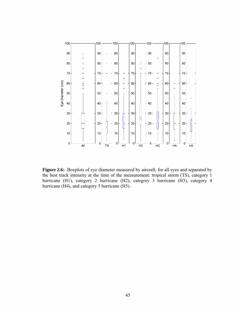
Figure 2.6: Boxplots of eye diameter measured by aircraft, for all eyes and separated by the best track intensity at the time of the measurement: tropical storm (TS), category 1 hurricane (H1), category 2 hurricane (H2), category 3 hurricane (H3), category 4 hurricane (H4), and category 5 hurricane (H5).

45

Figure 2.7: Boxplots of maximum sustained winds during 6 hr periods containing eye diameter measurements from aircraft, for all cases and separated by the eye diameter: <10 nmi, 10-20 nmi, 20-30 nmi, 30-40 nmi, 40-50 nmi, and >50 nmi.

46

Figure 2.8: Boxplots of maximum sustained winds during 6 hr periods containing eye diameter measurements from aircraft, for all eyes and separated by eye type: elliptical (EL), circular (CI), and concentric (CO).

47

Figure 2.9: Eye diameter based on the time it was observed in hours since TC genesis. Top left panel contains all eye diameter measurements, top right contains circular eyes, bottom left contains elliptical eyes, and bottom right contains concentric eyes. Genesis determined by the first entry in the TC best track. Colors represent the intensity category at the time of the eye diameter measurement: tropical storms and weaker are purple, Category 1 hurricanes are dark blue, Category 2 hurricanes are light blue, Category 3 hurricanes are green, Category 4 hurricanes are orange, and Category 5 hurricanes are magenta.

48

Figure 2.10: Eye diameter based on the time it was observed relative to the time of maximum intensity. Top left panel contains all eye diameter measurements, top right contains circular eyes, bottom left contains elliptical eyes, and bottom right contains concentric eyes. Time has been normalized to a -1..1 scale based on the total TC best track lifetime before and after maximum intensity. Colors represent the intensity category at the time of the eye diameter measurement: tropical storms and weaker are purple, Category 1 hurricanes are dark blue, Category 2 hurricanes are light blue, Category 3 hurricanes are green, Category 4 hurricanes are orange, and Category 5 hurricanes are magenta.

49

Figure 2.11: Series of histograms of intensity measured by maximum sustained wind (MSW, in kt). The data subset contained in each histogram is determined by eye diameter (in six 10 nmi bins) and time (normalized relative to lifetime maximum intensity). The six eye diameter bins are arranged in rows from largest (top row) to smallest (bottom row). The four columns represent different periods in the TC lifecycle based on lifetime maximum intensity, with the first two columns representing the time between the beginning of the TC lifecycle and maximum intensity, and the last two columns representing the time between maximum intensity and the end of the TC lifecycle. MSW (in kts) is represented on the horizontal axis, with the number of eye diameter estimates at that intensity (for each diameter and time bin) on the vertical axis. Two numbers listed in top right corner of each histogram represent the total number of eye estimates in each histogram (top) and median intensity in each histogram (bottom, in kt).

50

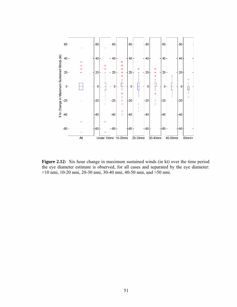
Figure 2.12: Six hour change in maximum sustained winds (in kt) over the time period the eye diameter estimate is observed, for all cases and separated by the eye diameter: <10 nmi, 10-20 nmi, 20-30 nmi, 30-40 nmi, 40-50 nmi, and >50 nmi.

51

Figure 2.13: Eye diameter stratified by month. April, May, and December have aircraft reconnaissance fixes but no eye diameter estimates; no reconnaissance is available in the months of January, February and March.

52

Figure 2.14: Maps of aircraft reconnaissance eye diameter measurements by month, June-November. Eye type represented by marker shape: circles for circular eyes, triangles for elliptical eyes, and squares for concentric eyes. Eye diameter in nmi represented by marker color: magenta < 10 nmi; 10 nmi ≤ orange < 20 nmi; 20 nmi ≤ green < 30 nmi; 30 nmi ≤ light blue < 40 nmi; 40 nmi ≤ dark blue < 50 nmi; purple ≥ 50 nmi.

53

Figure 2.15: Aircraft reconnaissance eye diameter estimates for all cases, and separated by latitude bands in which the estimates were observed: south of 15 degrees latitude, 15-20 degrees latitude, 20-25 degrees latitude, 25-30 degrees latitude, 30-35 degrees latitude, and north of 35 degrees latitude.

54

Chapter 3

EFFECTS OF VORTEX STRUCTURE ON THE DIABATICALLY-INDUCED

INTENSIFICATION OF TROPICAL CYCLONES

3.1 Overview

The purpose of this project is to see what conclusions can be drawn about the

relationships between the vortex structure, the diabatic heating, and the temperature and

tangential wind tendencies in idealized tropical cyclones. The theoretical argument is

based on the balanced vortex model, in particular on the associated geopotential tendency

equation. This is a second-order partial differential equation containing the diabatic

forcing and three spatially varying coefficients: the static stability, the baroclinicity, and

the inertial stability. Under the simplifying assumptions that baroclinic effects can be

neglected and that diabatic heating and the associated response is confined to the first

internal mode, the geopotential tendency equation reduces to a radial structure equation.

This is a second-order ordinary differential equation that can be solved numerically for

various vortex profiles. These solutions illustrate how the vortex response to diabatic

heating depends on whether this heating lies in the low inertial stability region outside the

radius of maximum wind or in the high inertial stability region inside the radius of

maximum wind, and how that response is modified by vorticity skirts.

55

The idealized tropical cyclone is extremely sensitive to the placement of the

diabatic heating relative to the vortex profile. Any heating contained within the radius of

maximum wind produces a sharp increase in intensity. Heating confined to the vorticity

skirt also intensifies the vortex, though not as rapidly as heating within the radius of

maximum wind. Heating located outside the vorticity skirt does not act to intensify the

tropical cyclone. The vortex increases intensity more than strength with heating located

at least partially within the radius of maximum wind, increases both approximately

equally for heating within the vorticity skirt, and increases strength without increasing

intensity for heating located outside the vorticity skirt.

3.2 Introduction

3.2.1 Background

The destructive potential of TCs is dependent on their size, strength, and intensity,

among other factors. Merrill (1984) defined intensity according to the extremes

measured in the TC circulation (usually MSW or MSLP), strength as the average wind

speed in the TC circulation, and size as the outermost extent of the TC circulation

(usually R34 or ROCI). Figure 3.1 uses a radial plot of tangential wind speed to illustrate

changes in intensity, strength, and size. Strength includes aspects of both intensity and

size, but can change while both other measures remain constant, and can be measured

with an average wind speed or some measure of kinetic energy (KE). Strength is also

dependent on the range of radii chosen for averaging.

The relationships between different aspects of TC structure are complex and have

been studied extensively over the years. In general, measures of size or outer core

strength are only weakly correlated to intensity (Merrill 1984, Weatherford and Gray

56

1988b) while inner core strength shows higher correlation to intensity (Croxford and

Barnes 2002). These relationships are further complicated by the tropical cyclone

environment (Merrill 1984, Hill and Lackmann 2009).

Ooyama (1969), using an axisymmetric, hydrostatic, gradient balanced, three-

layer model, produced the first success in modeling the TC lifecycle. While not

appropriate for examining individual cases, the ‘typical’ TC lifecycle produced with this

simple model allows us some perspective on the challenges encountered by researchers

looking to establish relationships between different aspects of TC structure. The results

of a typical case are summarized in Figure 3.2, which shows the time evolution of the

maximum tangential wind, the radius of maximum tangential wind, the radius of

hurricane force wind (64 kt, R64), the radius of gale force wind (34 kt, R34), the radius

of maximum upward Ekman pumping at the top of the boundary layer, and the minimum

surface pressure. The storm intensifies from 10 ms-1 to 58 ms-1 in 134 hr, after which the

maximum wind slowly decreases while the size of the storm continues to grow, as

represented by the outward movement of both R34 and R64. The increase in storm

strength is illustrated in Figure 3.3, which depicts the time evolution of the integrated KE

(IKE) inside radii of 100, 200, 500, and 1000 km. Note that, after the peak wind speed at

134 hr, there is continued rapid growth in the IKE inside 1000 km. The inner radii show

a leveling off of IKE late in the lifecycle, or even a reduction in IKE inside 100 km.

These changes do not occur until a day or more past the peak intensity time of 134 hr and

become less noticeable at larger radii. After 100 hr, less than half of the IKE within 1000

km is actually coming from the region within 200 km.

57

Another way to summarize this typical case is with a K-Vmax diagram, i.e., a

diagram in which the ordinate is the IKE inside a radius of 1000km and the abscissa is

the MSW. The time evolution of Ooyama’s typical case is shown by the multicolored

curve in the K-Vmax diagram shown in Figure 3.4. The lifecycle has been broken into

three stages: incipient (0-60 hr), deepening (60-134 hr), and mature (134-216 hr). As can

be seen in Figure 3.4, evaluating TC structure from MSW alone is inadequate. For

example, the TC has an MSW of approximately 44 ms-1 at around 96 hr and 216 hr, but

these two times have IKE differing by approximately a factor of six. At the first time the

TC is small and in the deepening stage, while at the second it is large and in the mature

stage. The reliance of the Saffir-Simpson scale on MSW has led to proposals by Powell

and Reinhold (2007) and Maclay et al. (2008) for a two-parameter storm classification

based on MSW and IKE.

While the multicolored curve in Figure 3.4 shows a typical TC lifecycle in the K-

Vmax plane, considerable variability from this curve can occur in real and model TCs. For

example, Hurricane Inez (1966), described in detail by Hawkins and Imbembo (1976)

and Hawkins and Rubsam (1967), was a small intense hurricane whose R64 and R34 near

the time of peak intensity were approximately half those of the typical case shown in

Figure 3.2. Even more extreme cases of small intense typhoons occur in the western

Pacific (e.g., see Arakawa (1952), Brand (1972), Merrill (1984), Weatherford and Gray

1988a,b, Harr et al. 1996). A classic example of a small intense TC is Cyclone Tracy,

which had an R34 of only 50 km when it struck Darwin, Australia in December 1974.

These small intense storms are represented by the purple region in the lower right of

Figure 3.4 with the label “strong dwarfs.” Proceeding to the purple region in the upper

58

right of Figure 3.4, we have designated this area “strong giants.” The western Pacific’s

mature supertyphoons often fall into this category, having large MSW and IKE

simultaneously. The classic example of these storms is Super Typhoon Tip (1979), as

described by Dunnavan and Diercks (1980). At its most intense Tip had MSW of 85 ms-1

and an R64 more than double the typical case shown in Figure 3.2, with an R34 of over

1100 km placing its IKE well off the upper edge of Figure 3.4. Finally the purple region

in the upper left of Figure 3.4 is labeled “weak giants,” which are tropical depressions or

tropical storms that, although not reaching hurricane intensity, can become quite large

and produce copious rainfall. Examples of these systems can again be found in the

western Pacific, and present particular challenges to those attempting to define

relationships between size, strength and intensity (Cocks and Gray 2002).

Internal dynamics can cause divergence from the typical main sequence in Figure

3.4, of which two possibilities are discussed below. The first is potential vorticity mixing

(Schubert et al. 1999, Kossin and Eastin 2001, Hendricks et al. 2009, Hendricks and

Schubert 2010). This process, which is often associated with polygonal eyewalls, tends

to reduce MSW but leave IKE relatively unchanged. A second source of variability from

the typical main sequence is a concentric eyewall cycle, a process in which intensification

is interrupted by the formation of an outer eyewall, the decay of the inner eyewall, and

finally the contraction of the outer eyewall (Willoughby et al. 1982, Houze et al. 2007,

Rozoff et al. 2008, Terwey and Montgomery 2008). The K-Vmax signature of a concentric

eyewall cycle for an intense TC is shown schematically by the dotted curve near the

center of Figure 3.4. Maclay et al. (2008) found concentric eyewall cycles to be a

primary mechanism for increasing IKE. Their study used aircraft reconnaissance flight-

59

level winds within a radius of 200 km for calculating IKE, with the resulting K-Vmax

points displayed in Figure 3.5. Fitting a power series to the data points explained 82% of

the variance between MSW and IKE, without examining the lifecycle of individual TCs.

However, once the TC lifecycle was considered distinct patterns emerged. Figure 3.6

shows the time evolution of K’-Vmax for six individual TCs, where K’ is the deviation of

the observed IKE from the IKE predicted by the best fit of the observed Vmax. The

“horizontal question mark” referred to in Figure 3.6 is a pattern Maclay et al. (2008)

identified in K’ in particular TCs, in which a TC starting to intensify may experience a

slight decrease in K’, rapid intensification leads to a large decrease in K’, and once peak

intensity is reached K’ increases. They found that TCs generally increase MSW without

increasing IKE, or increase IKE without increasing MSW.

This study examines the response of an idealized tropical cyclone to the location

of diabatic heating, in terms of changes in both MSW and IKE. The theoretical argument

is based on the balanced vortex model, in particular on the associated geopotential

tendency equation. This is a second-order partial differential equation containing the

diabatic forcing and three spatially varying coefficients: the static stability, the

baroclinicity, and the inertial stability. Under the simplifying assumptions that baroclinic

effects can be neglected and that diabatic heating and the associated response is confined

to the first internal mode, the geopotential tendency equation reduces to a radial structure

equation. This is a second-order ordinary differential equation that can be solved

numerically for various vortex profiles. The idealized vortex profile in this study is

assumed to be Gaussian, and the diabatic heating is assumed to lie in an annular ring.

The solutions illustrate how the vortex response to diabatic heating depends on whether

60

the heating lies in the low inertial stability region outside the RMW or in the high inertial

stability region inside the RMW, and how that response is modified by the vorticity skirt.

3.2.2 Chapter Overview

The project discussed in this chapter is based off experiments using the balanced

vortex model, which is described in Section 3.3. The structure of the diabatic forcing and

the Gaussian vortex are described in Sections 3.3.1 and 3.3.2, respectively. The

formulation of the integrated kinetic energy is presented in Section 3.3.3. The response

of the vortex to the radial placement of the diabatic heating is examined in Section 3.4, in

terms of the overlap of the heat source with the vorticity profile of the initial vortex. The

behavior of the vortex kinetic energy as well as a comparison of strengthening and

intensification is discussed in Section 3.4.1. Section 3.6 contains a summary of relevant

points and future work.

3.3 Balanced Vortex Model

We consider inviscid, axisymmetric, quasi-static, gradient-balanced motions of a

stratified, compressible atmosphere on an -plane. As the vertical coordinate we use f

( ppHz 0ln= ) , where gRTH 0= , with and denoting constant reference values

of pressure and temperature. The governing equations for the balanced vortex model are

0p 0T

rv

rvf

∂∂

=⎟⎠⎞

⎜⎝⎛ +

φ , (3.1)

( ) 0=∂∂

+⎟⎠⎞

⎜⎝⎛

∂∂

++∂∂

zvw

rrrvfu

tv , (3.2)

TTg

z 0

=∂∂φ , (3.3)

61

( ) 0=−∂∂

+∂

∂Hw

zw

rrru , (3.4)

pp cQ

HcRT

zTw

rTu

tT

=⎟⎟⎠

⎞⎜⎜⎝

⎛+

∂∂

+∂∂

+∂∂ , (3.5)

where and are the radial and tangential components of velocity, is the ‘vertical

velocity’,

u v w

φ is the geopotential, is the constant Coriolis parameter, and is the

diabatic heating. Equations (3.1)-(3.5) constitute a system of five equations in the six

unknowns , , ,

f Q

u v w φ , T , , so obviously an additional “parameterization” relating Q

to the other unknowns is required for closure. However, adding a sixth equation in this

way has an important disadvantage – our confidence that this sixth equation is an

accurate description of nature is much lower than our confidence that (3.1)-(3.5) are

accurate descriptions of nature. Because of this, we here attempt to see what conclusions

can be drawn about the relationships between the vortex structure, the temperature and

tangential wind tendencies, and the diabatic heating, without making use of such

comparatively uncertain parameterization relations.

Q

As a hurricane evolves, the spatial distributions of the static stability,

baroclinicity, and inertial stability change. The changes in the inertial stability can be

particularly large, with important implications for the spatial distribution of tendencies of

the wind and mass fields. To isolate the important role of changes in the inertial stability,

we seek solutions of (3.1)-(3.5) under the assumption that the baroclinic terms ( )zvw ∂∂

and ( rTu ∂∂ ) can be neglected. Near the vortex core of a hurricane the baroclinic terms

do play an important role in producing an outward tilt to the eyewall updraft, so the

present analysis will not capture this effect. However, an important advantage of the

62

approach followed here is that it leads to insight about the role of vorticity skirts using

very simple mathematical methods. Thus, neglecting the baroclinic terms, we now

multiply the thermodynamic equation by 0Tg and the tangential wind equation by

( rvf 2+ ), and then make use of the gradient and hydrostatic relations to obtain

QTcgwN

z p

t

0

2 =+∂∂φ

, (3.6)

0ˆ 2 =+∂∂

ufr

tφ , (3.7)

where tt ∂∂= φφ denotes the geopotential tendency, and where the static stability and

the inertial stability are given by

⎟⎟⎠

⎞⎜⎜⎝

⎛+

∂∂

=Hc

RTzT

TgN

p0

2 , (3.8)

( )⎟⎠⎞

⎜⎝⎛

∂∂

+⎟⎠⎞

⎜⎝⎛ +=

rrrvf

rvff 2ˆ 2 . (3.9)

In the following analysis we shall consider to be a constant and to be a function

of

2N 2f̂

r only.

One way of proceeding from (3.6) and (3.7) is to eliminate tφ to obtain an

equation for the transverse circulation (Eliassen 1952, Shapiro and Willoughby 1982,

Schubert and Hack 1982). The solution of this transverse circulation equation yields the

radial and vertical velocity components, which can then be substituted into the tangential

wind and thermodynamic equations to obtain the tendencies of v and T . A more direct

route to the tendencies is obtained (Vigh and Schubert 2009) by using the continuity

63

equation to eliminate u and between (3.6) and (3.7), thereby obtaining the tendency

equation

w

QHzTc

gzHzr

t⎟⎟⎠

⎞φfr

⎜⎜⎝

⎛ˆrr

Np

t ⎟⎠⎞

⎜⎝⎛ −∂∂

=∂∂

⎟⎠⎞

⎜⎝⎛ −∂∂

+∂∂

∂∂ 11

02

2 φ . (3.10)

Equation (3.10) is a second order partial differential equation for tφ . To obtain boundary

conditions for (3.10) we assume that Q and vanish along the top and bottom

boundaries, so that (3.6) yields

w

0=∂∂

ztφ at Tzz ,0= . (3.11)

Since vanishes along the axis of symmetry and as u 0→ru ∞→r , (3.7) yields

=∂∂

rtφ 0=r , and 0→trφ as ∞→r . (3.12) 0 at

Here we consider only vortices with everywhere, which ensures that (3.10)-

(3.12) is an elliptic problem.

0ˆ >Nf

We now solve (3.10)-(3.12) via separation of variables, assuming that ( )zrQ , has

the vertical structure given below in (3.13). Then, it is easily shown that ( )zrTt , and

have the same vertical structure and that ( zrw , ) ( )zrt ,φ , ( )zrvt , , and have the

vertical structure given in (3.14).

( , )zru

( )( )( )

( )( )( )

⎟⎟⎠

⎞⎜⎜⎝

⎛⎟⎠⎞

⎜⎝⎛

⎟⎟⎟⎟

⎠

⎞

⎜⎜⎜⎜

⎝

⎛

=⎟⎟⎟

⎠

⎞

⎜⎜⎜

⎝

⎛

Tt z

zHz

wTQ

zrwzrTzrQ

πsin2

expˆ

ˆˆ

,,,

t

rrr

, (3.13)

64

( )( )( )

( )( )( )

⎥⎦

⎤⎢⎣

⎡⎟⎟⎠

⎞⎜⎜⎝

⎛−⎟⎟

⎠

⎞⎜⎜⎝

⎛⎟⎠⎞

⎜⎝⎛

⎟⎟⎟⎟

⎠

⎞

⎜⎜⎜⎜

⎝

⎛

=⎟⎟⎟

⎠

⎞

⎜⎜⎜

⎝

⎛

T

T

Tt

t

t

t

zz

Hz

zz

Hz

rurvr

zruzrvzr

ππ

πφφ

sin2

cos2

expˆˆ

ˆ

,,,

, (3.14)

The two vertical structure functions appearing in (3.13) and (3.14) are plotted in Figure

3.7. The blue curve is the vertical structure function ( )[ ] ( TzzHz )πsin2exp , which

reaches its maximum at , where is given by mzz = mz ( )TTm zHzz πππ 2tan 1 −+= − .

For km and km, we obtain 15=Tz 718.8=H 776.8=mz km, which yields a maximum

value of for the vertical structure function. The red curve is the vertical structure

function

596.1

( )[ ] ( ) [ ]( ) ( )[ ]TT zzHzH Tzzz ππ sin22 cosexp π− . Then, using the separable

forms (3.13) and (3.14) we can show that the hydrostatic, gradient wind, tangential wind,

and thermodynamic equations respectively imply that

( ) ( )rHz

zrTTg

tT

Tt φπ

πˆ

41ˆ

22

2

0⎟⎟⎠

⎞⎜⎜⎝

⎛+−= , (3.15)

( ) ( )dr

rdrvfrv t

tφ̂2ˆ

1−

⎟⎠⎞

⎜⎝⎛ += , (3.16)

( ) ( )dr

rdfru tφ̂ˆˆ 2−−= , (3.17)

( ) ( ) ( )⎟⎟⎠

⎞⎜⎜⎝

⎛−= rT

crQ

NTgrw t

p

ˆˆˆ

20

. (3.18)

Substituting (3.13) and (3.14) into (3.10) we find that the ordinary differential equation

for the radial structure of the temperature tendency is given by (3.21a), where

65

( )( ) ( ) 0

21

22

2

ˆ41

ˆ llrf

fHzrf

NrT

=⎟⎟⎠

⎞⎜⎜⎝

⎛+=

−π (3.19)

is the Rossby length. As ∞→r , ( ) frf →ˆ and ( ) 0ll →r

0

, the constant far-field value

which we shall assume is equal to 1000 km. One of the remarkable features of hurricanes

is the wide range of , which can shrink from this far-field value of 1000 km to less

than 10 km in the core. The boundary condition at

( )rl

=r is given by (3.21b). Since our

problem is to be solved numerically over a finite domain, we need to replace the

boundary condition r as 0ˆ →tT ∞→r with an approximate far-field boundary condition

at some large radius . In the far-field and b=r 0→Q̂ ( ) 0ll →r , so that (3.21a)

simplifies to

0ˆ1ˆˆ20

2

2

=−+ ttt T

rdrTd

drTd

l for large r . (3.20)

The solution of (3.20) consists of a linear combination of the zero order modified Bessel

functions, i.e., ( ) ( ) ( )0000ˆ ll rIrKrTt βα += , where α and β are constants. Since

( ) ∞→00 lrI as ∞→r , we require 0=β , so that ( ) ( )0ˆ lKt α= 0 rrT for large r . The

value of α depends on the details of the solution in the inner region, but it can be

eliminated by noting that ( ) ( )01ˆ lrKdrTd t −= 0lα , so that, at , br = drTd t̂ and

are related by (3.21c). In all the calculations shown here we have assumed km

and km, so that the factor in the large parentheses on the right-hand side of

(3.21c) is approximately (700 km)-1.

tT̂

1000=b

10000 =l

66

To summarize, the second order differential equation and the appropriate

boundary conditions for our problem are

p

tt c

QdrTd

rrdrdT

ˆˆˆ 2 =⎟

⎟⎠

⎞⎜⎜⎝

⎛− l , (3.21a)

0ˆ=

drTd t at 0=r , (3.21b)

( )( ) t

t TbK

bKdrTd ˆˆ

000

01⎟⎟⎠

⎞⎜⎜⎝

⎛−=

ll

l at br = . (3.21c)

Once is found from (3.21), the original fields ( )rTt̂ ( )zrTt , , ( )zrvt , , ( )zrt ,φ , , and

can be recovered from (3.13)-(3.18). Solutions of (3.21) reveal how the nonlocal

relationship between the diabatic heating

( zru , )

(rw , )z

( )rQ̂ and the temperature tendency ( )rTt̂ is

modulated by the vortex structure through the radial distribution of the Rossby length

. ( )rl

Understanding the nonlocal behavior of the solutions of (3.21) is a crucial part of

an overall understanding of the rapid intensification process. Vigh and Schubert (2009)

have solved (3.21) analytically for the special case in which ( )rl is piecewise constant

over two regions – the core and the far-field. They have shown that, when ( )rQ̂ is

localized in a region where ( )rl is small, it is possible for ( )rT to be large and localized

in the same region because the small values of

t̂

( )rl reduce the magnitude of the second

derivative term even though 2ˆ drt2Td is large. In the present study we consider radial

profiles of that are more complicated, i.e., profiles that have low values of ( )rl ( )rl in

67

the core and large values of ( )rl in the far-field, but a more gradual transition due to the

presence of a “vorticity skirt” outside the radius of maximum wind. Because of these

more complicated radial profiles of ( )rl , we shall solve (3.21) numerically.

If (3.21a) were solved on an infinite domain with the boundary condition

as

0ˆ →tTr

∞→r , then integration of (3.21a) would yield the integral relation

∫∞

0

T ∫∞

0

ˆˆ rdrcQ

pt =rdr , (3.22)

which states that the area-integrated temperature tendency is equal to the area-integrated

diabatic heating, even though ( )Q̂ r can be large and localized while can be small

and spread over a wide area. What is the analogue of (3.22) for our finite domain?

Integration of (3.21a), with use of the boundary conditions (3.21b) and (3.21c), yields

( )rTt̂

( )( ) ( ) ∫∫ =+ 0l

b

b

pt

b

t rdrcQbT

bKbbK

rdrT000

01

0

ˆˆˆl

l, (3.23)

where we have assumed that is large enough that ( ) 0ll ≈b . Although our numerical

solution for is obtained in the region ( )rTt̂ br ≤≤0 , suppose we extend it to infinity by

( )(( ) )(ˆ bTt )00

00ˆl

l

bKrK

rTt = for ∞<≤ rb . (3.24)

Integrating (3.24) we obtain

68

( )( ) ( )

( )( )

( )[ ]

( )( ) ( )bTbK

bbK

drdr

rrKdbK

bT

rdrrKbKbT

rdrT

t

b

t

b

t

bt

ˆ

ˆ

ˆˆ

00

010

01

00

0

0000

l

ll

l

l

l

ll

=

−=

=

∫

∫∫∞

∞∞

. (3.25)

Since the right hand side of (3.25) is equal to the second term in (3.23), and since we

have assumed that for 0ˆ =Q ∞<≤ rb , we can simplify (3.23) to

∫∫∫∞∞

=+00

ˆˆˆ rdrcQrdrTrdrT

pbt

b

t , (3.26)

which is equivalent to the infinite domain result (3.22). Thus, in the sense that the finite

domain result is extended to infinity according to (3.24), the integral relation (3.22) is

preserved.

3.3.1 Diabatic Heating

To specify the term in (3.21) we assume that the storm has formed an eye,

so that the diabatic heating has the form of an annular ring with smooth edges, i.e.,

( )rQ̂

( )( ) ( )[ ]

( ) ( )[ ]⎪⎪⎪

⎩

⎪⎪⎪

⎨

⎧

∞≤≤≤≤−−≤≤≤≤−−≤≤

=

rrrrrrrrrSrrrrrrrrrrSrr

QrQ ew

4

43343

32

21122

1

ˆ0ˆˆˆˆˆˆˆ1ˆˆˆˆˆˆ00

ˆˆ , (3.27)

where is the cubic interpolating function satisfying ( ) 32 231 sssS +−= ( ) 10 =S ,

, and , , , are specified constants. The eyewall ( )1 =S 0 ( ) ( ) 010 =′=′ SS 1̂r 2̂r 3̂r 4̂r

69

diabatic heating, denoted by , is determined from , , , by imposing the

constraint that the domain-averaged diabatic heating is fixed, i.e.,

ewQ̂ 1̂r 2̂r 3̂r 4̂r

( ) 2.0ˆ2

02 =∫

b

p

rdrc

rQb

K day-1. (3.28)

Substituting (3.27) into (3.28), and performing the integration, we obtain

⋅= Gc

Q

p

ewˆ

(0.2 K day-1), (3.29)

where the geometrical factor is given by G

( ) ( )2

2̂r

22

12

4432

3

2

4ˆ3ˆ3ˆˆ4ˆ310

rrrrrbG

+−++=

21 ˆˆ rr ˆ3r+

1̂r

. (3.30)

From (3.29) and (3.30) we can compute once and , , , are specified.

Plots of

ewQ̂ b 3̂r 4̂r

( ) pcrQ̂ , computed using the parameters listed for the highlighted cases in Table

3.1, are shown in Figure 3.8.

3.3.2 Vortex Profile

We now consider some sample solutions of (3.21). In order to specify the ( )rl

factor in (3.21), we shall consider the family of Gaussian vortices given by

( ) ( )[ ]22exp12

arr

rv −−Γ , (3.31) =π

where and are constants. Since Γ a Γ→vrπ2 as ∞→r , the constant Γ represents

the circulation at large radii. The relative vorticity field associated with (3.31) is given

by

70

( ) ( )222 exp ar

ar −

Γ=π

ζ , (3.32)

so the constant is the e-folding radius of the vorticity distribution. The maximum wind

occurs at and has the value

a

.1 arm 1209≈ ( )avm π263817.0 Γ≈ . Using (3.8), (3.14) and

(3.31), we obtain

( )( )[ ] [ ]

0

21

222

222

2

expexp1ll

⎟⎟⎟⎟⎟

⎠

⎞

⎜⎜⎜⎜⎜

⎝

⎛

⎟⎟⎠

⎞⎜⎜⎝

⎛−

Γ+⎟⎟

⎠

⎞⎜⎜⎝

⎛−−

Γ+

=ar

afar

rf

fr

ππ

. (3.33)

For all the results presented here we have chosen a sample ‘base’ vortex with , , ,

and listed in Table 3.2. Figure 3.9 shows

mr mv a

Γ ( )rv , ( )rζ , and ( )rl profiles for the ‘base’

vortex given in the shaded row of Table 3.2. With this radial vortex profile and the radial

profiles of diabatic heating presented in Figure 3.8 we can study the vortex response to

heating in terms of changes in intensity and strength.

3.3.3 Integrated Kinetic Energy

The IKE of the idealized vortex profiles is calculated to allow for comparison

with the observed IKE in Maclay et al. (2008). The IKE is calculated from a thin disk

centered on an assumed flight level of 700 mb, using the equation

∆ , (3.34)

where 0.9 kg m-3, ∆ 1 km, 200 km, and u and v are evaluated at the 700

mb level. Maclay et al. (2008) also found a best fit relationship between IKE and Vmax

from the aircraft reconnaissance,

71

3 10 . , (3.35)

where KM is the best fit IKE and vM is the maximum flight level wind (Maclay et al.

2008). The relationship explained 82% of the variance in their data, though significant

variability in IKE was noted for a given intensity. The solid curve in Figure 3.5 shows

the best fit relationship to the data, while the dashed curve shows the square of vM.

Table 3.2 lists the K for the initial Gaussian vortex profiles, K0, as well as the best

fit KM for the initial vM. In general K0 is less than KM for the initial vortices, with values

of K0 exceeding the corresponding KM occurring starting at an RMW of 50 km. This

behavior is unsurprising given the lack of size parameter in KM. The idealized Gaussian

vortex profile also contributes to the smaller values of K0. The vorticity skirt in observed

TCs is more substantial than in their Gaussian counterparts, leading to stronger winds and

a higher IKE, as well as the added complications of observed secondary wind maxima

(Mallen et al. 2005).

3.4 Changes in Vortex Structure

The following discussion is broken into five general types of cases based on the

location of the heating in relation to the initial vortex profile. The cases are broken into

those with heating: 1) confined inside the RMW, 2) stretching across the RMW, 3)

confined inside the vorticity skirt, 4) partially inside the vorticity skirt, and 5) outside the

vorticity skirt. The outer edge of the vorticity skirt has been defined as the location

where the vorticity equals f, as indicated by in Table 3.2. Alternately, calculates

the outer edge of the vorticity skirt based on the location where the vorticity decreases to

one hundredth of the maximum vorticity. For the Gaussian vortex profiles this reduces

72

to a function of rm only, regardless of the strength of the vortex, and produces skirt

edges that are quite large, particularly for larger vortices. For the rest of the discussion

the vorticity skirt is considered to extend to . For the ‘base’ vortex R3V3 (Figure 3.9),

six heating profiles have been selected to highlight the differing types. The odd cases

DH3-DH13 each represent a heating profile that is 10 km further from the vortex center

than the previous odd-numbered case (Figure 3.8). Case DH3 is type 1, DH5 is type 2,

DH7 is type 3, and both DH9 and DH11 are type 4. DH9 lies almost entirely within the

vorticity skirt, while DH11 lies almost entirely outside the vorticity skirt. Case DH13 is

type 5 as it lies entirely outside the vorticity skirt.

The vortex structure after the application of heating is examined by computing the

resulting vortex after six hours. Tables 3.3-3.5 contain qualitative comparisons of the

RMW, Vmax, and IKE, respectively. The tables are calculated by normalizing the six hour

values of rm, vm, and K by their initial values. Blank spaces represent nearly equal

quantities, smaller six hour values by increasing ‘-’ designations (~-,-,--), and larger six

hour values by increasing ‘+’ designations (~+,+,++). Each measure is considered

separately relative to its initial value, then the relative increases between measures are

compared.

Heating within the RMW produces the contraction of RMW and increase of Vmax

seen in previous studies (e.g., Shapiro and Willoughby 1982, Vigh and Schubert 2009).

Heating across the RMW or contained completely within the vorticity skirt continues to

produce an increase in Vmax, while the RMW expands. Heating partially or completely

outside the vorticity skirt shows no noticeable effect on the RMW and either no change

or a slight decrease in Vmax. The IKE is increased in all cases, with larger increases seen

73

as the heating approaches the vortex center. Note that the constraint (3.28), together with

the assumed vertical structure of the heating given by (3.13), means that the total energy

generation given by the right hand side of the total energy principle

∫∫ ∫∫ −− =⎟⎠⎞

⎜⎝⎛ + dzdrrQedzdrreTcv

dtd HzHz

p2

21 . (3.36)

is the same for each heating profile shown in Figure 3.8. However, the fraction of the

total energy generation that is partitioned to KE generation is dependent on the position

of the heating relative to the inertial stability. An “energy efficiency” interpretation of

this effect has been given by Hack and Schubert (1986).

The individual cases DH3, DH5, DH7, DH9, DH11, and D13 are showcased in

Figures 3.10-3.15. The first panel depicts the initial vortex and heating profiles. The

next five panels show the vortex response, with and in the second panel,

in the third, in the fourth panel, in the fifth, and in the sixth panel.

The fourth panel also contains

( )rvtˆ ( )rtζ̂

( )rv at t = 6 hr, and the sixth panel similarly contains

( )rζ at t = 6 hr. In all cases the temperature tendency, geopotential tendency, and

vorticity change is maximized along the inner edge of the heating profile. The maximum

inflow and vertical velocity is found along the outer edge of the heating profile.

For the type 1 case DH3 the most intense response is seen (Figure 3.10). The

tangential wind tendency is large, with the maximum collocated with the inflow

maximum, inside the original RMW. The vortex contracts as it intensifies, and the vortex

profile inside the heating hollows (Shapiro and Willoughby 1982, Kossin and Eastin

2001). Similar behavior is seen in the type 2 case DH5 (Figure 3.11), except the

74

superposition of the tangential wind tendency with the initial vortex leads to an expansion

of the RMW. While the RMW has shifted outside the initial RMW, it is still located

radially inward from the inflow maximum along the outer edge of the heating.

For the type 3 case DH7 (Figure 3.12), where the heating is outside of the RMW

but contained within the vorticity skirt, the vortex still expands and intensifies. Both the

tangential wind tendency and the resultant 6 hr tangential wind profile maximize radially

inward from the inflow maximum. A secondary maximum is still present in the relative

vorticity but it no longer overpowers the vorticity maximum in the center. Significant

hollowing of the vortex is no longer seen. As the heating progresses to the outer portion

of the vorticity skirt, the vortex stops expanding and intensifying.

As the heating progresses further outward into the type 4 cases, the heating ceases

to have a significant impact on the vortex intensity or RMW. For the type 4 case DH9

(Figure 3.13), the heating is mostly contained within the vorticity skirt. The inflow

maximum lies just outside the vorticity skirt, and the tangential winds increase nearly

uniformly through the area of heating. For the type 4 case DH11 (Figure 3.14), the

heating is mostly outside of the vorticity skirt. Some interaction of the heating with the

vorticity skirt is still visible in the vorticity tendency, but the tangential wind tendency is

approaching the response for heating outside the skirt. The type 5 case DH13 (Figure

3.15) has heating completely outside the vorticity skirt, with the vorticity tendency

showing a flat increase in the heating region and the tangential wind tendency showing an

increase proportional to the inflow. Despite the lack of significant change in MSW or

RMW, IKE continues to increase in all these cases due to the increase in tangential winds

extending radially outward from the heating.

75

3.4.1 Vortex Response: Strength and Intensity

While the IKE increases in all cases, as seen in Table 3.5, the behavior can be

assessed based on the location of the diabatic forcing. When the heating is fully or

partially confined within the RMW, IKE increases much less than MSW. The increase in

IKE is only a fraction of the increase predicted using (3.35). The response moves the

vortex structure further towards the right of the best fit KM curve in Figure 3.5, and

resembles the deepening stage in Figure 3.4.

When the heating is confined within the vorticity skirt region, both MSW and IKE

increase slightly. The increases normalized by their initial values remain close, and the

change in IKE is close the change in the best fit KM. This is consistent with a TC

approaching its peak intensity in Figure 3.4. As the heating approaches the outer edge of

the vorticity skirt, the MSW decreases slightly while the IKE continues to increase,

shifting the vortex to the left of the best fit KM curve in Figure 3.5 and more consistent

with a storm that has reached peak intensity in Figure 3.4. When the heating falls

partially or fully outside the vorticity skirt region, IKE increases without an associated

change in MSW or RMW.

3.5 Summary

This study examined the response of an idealized vortex to a ring of diabatic

heating in the balanced vortex model. The vortex response was assessed based on the

location of the heating: within the RMW, inside the vorticity skirt, or outside the vorticity

skirt. The changes in intensity and strength were assessed and considered in relation to

the K-Vmax figure (Figure 3.4) based on the “typical” TC lifecycle modeled by Ooyama

(1969).

76

The balanced vortex model was reduced to a second order partial differential

equation in terms of the geopotential tendency, as opposed to the traditional approach of

solving for the secondary circulation. Assuming the diabatic heating to have the vertical

structure given in (3.13) allowed for separation of variables, reducing the model to a

second order differential equation (3.21) which could be solved numerically on a finite

domain given radial profiles of the Rossby length and diabatic heating. Gaussian vortex

profiles allowed for the effects of the presence of a vorticity skirt to be studied when an

annular ring of heating is applied to the vortex.

The vortex response, particularly in intensity, is extremely sensitive to the

placement of the diabatic heating. Any heating contained within the RMW produces a

sharp increase in intensity, corresponding to the deepening stage in Figure 3.4 and also

providing the most likely scenario for rapid intensification of the idealized TC.

Depending on the combination of vortex and diabatic heating profiles, the intensification

caused by constraining the heating within the RMW could reach unrealistic rates. The

increase in strength was less pronounced for these cases than the increase in intensity.

Despite having relatively smaller increases in strength than intensity, the placement of the

heating within the high inertial stability region within the RMW was still the most

efficient overall at converting the energy from the heat source into KE.

Heating within the vorticity skirt was equally efficient at increasing both the

intensity and strength of the vortex, with smaller increases in both compared to the

response to heating within the RMW. As the heating approached the outer edge of the

vorticity skirt the intensity was seen to decrease slightly, though the strength still

increased slightly. Heating outside the vorticity skirt had a negligible impact on the

77

intensity and a slight increase in strength. The progression of the heating radially

outward from the RMW corresponded more with a shift from a deepening to a mature

TC, and acted as a brake on the intensification rate.

Accurate representation of the heating in relation to the vortex profile may

provide a useful metric for predicting TC intensity and structural changes. This simple

idealized model can be expanded to incorporate more complex vortex and heating

profiles and solved numerically with the framework provided in the study. This

framework allows for further research into the effects of vortex hollowness and

concentric eyewalls.

The ability to solve this model numerically allows for the inclusion of vortex and

heating profiles generated from both dynamical models and observations to be assessed

in this idealized framework. Future work examines the vortex response with both models

and observations, allowing for the development of a simple predictive tool for intensity

and a diagnostic tool for dynamical model development.

78

Table 3.1: Specifications of diabatic heating ( )rQ̂

2̂r 3̂r used in model. The first column,

DH#, uniquely identifies the bounding radii , , , and the area factor used in

any given case. The last column, 1̂r 4̂r G

pew cQ̂ , indicates the maximum value of the eyewall heating based on (3.29). The heating profiles specified by the six highlighted cases are shown in Figure 3.8.

Label 1̂r (km) 2̂r (km) 3̂r (km) 4̂r (km) G pew cQ̂ (K day-1)

DH1 0 5 15 20 3333.33 666.67 DH2 5 10 20 25 2222.22 444.44 DH3 10 15 25 30 1666.67 333.33 DH4 15 20 30 35 1333.33 266.67 DH5 20 25 35 40 1111.11 222.22 DH6 25 30 40 45 952.38 190.48 DH7 30 35 45 50 833.33 166.67 DH8 35 40 50 55 740.74 148.15 DH9 40 45 55 60 666.67 133.33 DH10 45 50 60 65 606.06 121.21 DH11 50 55 65 70 555.56 111.11 DH12 55 60 70 75 512.82 102.56 DH13 60 65 75 80 476.19 95.24 DH14 65 70 80 85 444.44 88.89 DH15 70 75 85 90 416.67 83.33

79

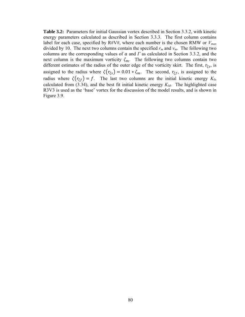
Table 3.2: Parameters for initial Gaussian vortex described in Section 3.3.2, with kinetic energy parameters calculated as described in Section 3.3.3. The first column contains label for each case, specified by R#V#, where each number is the chosen RMW or Vmax divided by 10. The next two columns contain the specified rm and vm. The following two columns are the corresponding values of and Γ as calculated in Section 3.3.2, and the next column is the maximum vorticity . The following two columns contain two different estimates of the radius of the outer edge of the vorticity skirt. The first, , is assigned to the radius where 0.01 . The second, , is assigned to the radius where . The last two columns are the initial kinetic energy K0, calculated from (3.34), and the best fit initial kinetic energy KM. The highlighted case R3V3 is used as the ‘base’ vortex for the discussion of the model results, and is shown in Figure 3.9.

80

Labe

lr m

(km

)v

m (m

s-1)

a (k

m)

Γ (1

05 m2 s-1

)ζ m

(10-3

s-1)

r ζs (

km)

r ζf (

km)

K0

(1016

J)K

M (1

016 J)

R1V

110

108.

928.

783.

5119

.14

18.3

90.

020.

22R1

V2

1020

8.92

17.5

77.

0319

.14

19.8

40.

070.

82R1

V3

1030

8.92

26.3

510

.54

19.1

420

.63

0.15

1.75

R1V

410

408.

9235

.13

14.0

519

.14

21.1

80.

272.

99R1

V5

1050

8.92

43.9

217

.57

19.1

421

.60.

424.

55R2

V1

2010

17.8

417

.57

1.76

38.2

833

.67

0.05

0.22

R2V

220

2017

.84

35.1

33.

5138

.28

36.7

80.

210.

82R2

V3

2030

17.8

452

.75.

2738

.28

38.5

0.47

1.75

R2V

420

4017

.84

70.2

77.

0338

.28

39.6

80.

832.

99R2

V5

2050

17.8

487

.84

8.79

38.2

840

.56

1.3

4.55

R3V

130

1026

.76

26.3

51.

1757

.43

47.5

10.

10.

22R3

V2

3020

26.7

652

.72.

3457

.43

52.4

80.

390.

82R3

V3

3030

26.7

679

.05

3.51

57.4

355

.18

0.87

1.75

R3V

430

4026

.76

105.

44.

6957

.43

57.0

31.

552.

99R3

V5

3050

26.7

613

1.76

5.86

57.4

358

.41

2.43

4.55

R4V

140

1035

.69

35.1

30.

8876

.59

60.4

40.

150.

22R4

V2

4020

35.6

970

.27

1.76

76.5

967

.35

0.59

0.82

R4V

340

3035

.69

105.

42.

6376

.59

71.0

51.

331.

75R4

V4

4040

35.6

914

0.54

3.51

76.5

973

.59

2.36

2.99

R4V

540

5035

.69

175.

674.

3976

.59

75.5

3.68

4.55

R5V

150

1044

.61

43.9

20.

795

.73

72.4

70.

20.

22R5

V2

5020

44.6

187

.84

1.41

95.7

381

.52

0.8

0.82

R5V

350

3044

.61

131.

762.

1195

.73

86.3

1.79

1.75

R5V

450

4044

.61

175.

672.

8195

.73

89.5

43.

192.

99R5

V5

5050

44.6

121

9.59

3.51

95.7

391

.98

4.98

4.55

81

Table 3.3: Change in RMW after adding six hour tendencies, as measured by the normalized RMW rmn. Blank space indicates 0.99 1.01. RMWs smaller than the initial RMW are indicated in three stages: 0.9 0.99 is ‘~-‘, 0.5 0.9 is ‘-‘, and 0.5 is ‘--’. RMWs larger than the initial RMW are likewise indicated in three stages: 1.01 1.1 is ‘~+‘, 1.1 2.0 is ‘+‘, and 2.0 is ‘++’.

rmn DH

1

DH

2

DH

3

DH

4

DH

5

DH

6

DH

7

DH

8

DH

9

DH

10

DH

11

DH

12

DH

13

DH

14

DH

15

R1V1 - ~+ + R1V2 - + + R1V3 - + + R1V4 - + + R1V5 - + + R2V1 - - + + R2V2 - - + + R2V3 - - ~+ + + R2V4 - ~- ~+ + + R2V5 - ~- ~+ + + R3V1 - - - + + + R3V2 - - - + + + R3V3 - - - + + + R3V4 - - - + + + R3V5 - - - ~- + + + R4V1 -- - - - ~- ~+ + + + R4V2 -- - - - ~- ~+ + + + R4V3 -- - - - ~- ~+ + + + R4V4 -- - - - ~- ~+ + + + R4V5 -- - - - ~- ~+ + + + R5V1 -- -- - - - - ~- ~+ + + + R5V2 -- -- - - - - ~- ~+ + + + R5V3 -- -- - - - - ~- ~+ + + + R5V4 -- -- - - - - ~- ~+ + + + R5V5 -- -- - - - - ~- ~+ + + +

82

Table 3.4: Same as Table 3.3 expect for changes in maximum tangential winds as represented by normalized Vmax, vmn.

vmn DH

1

DH

2

DH

3

DH

4

DH

5

DH

6

DH

7

DH

8

DH

9

DH

10

DH

11

DH

12

DH

13

DH

14

DH

15

R1V1 ++ ++ + R1V2 ++ ++ + R1V3 ++ ++ + R1V4 ++ ++ + R1V5 ++ ++ + R2V1 ++ ++ ++ + + R2V2 ++ ++ ++ + + R2V3 ++ ++ ++ + + ~- R2V4 ++ ++ ++ + + ~- R2V5 ++ ++ ++ + + ~- R3V1 ++ ++ ++ ++ + + + R3V2 ++ ++ ++ ++ + + + R3V3 ++ ++ ++ ++ + + + ~- R3V4 ++ ++ ++ ++ + + + ~- R3V5 + + + + + + + ~- R4V1 ++ ++ ++ ++ ++ + + + + R4V2 ++ ++ ++ ++ ++ + + + + R4V3 ++ ++ ++ ++ + + + + + ~- R4V4 ++ ++ ++ ++ + + + + + ~- R4V5 ++ ++ ++ ++ + + + + + ~- ~- R5V1 ++ ++ ++ ++ ++ ++ + + + + + R5V2 ++ ++ ++ ++ ++ + + + + + + R5V3 ++ ++ ++ ++ ++ + + + + + + ~- R5V4 ++ ++ ++ ++ + + + + + + + ~- R5V5 ++ ++ ++ ++ + + + + + + + ~- ~-

83

Table 3.5: Same as Table 3.3 expect for changes in kinetic energy as represented by normalized IKE, Kn.

Kn DH

1

DH

2

DH

3

DH

4

DH

5

DH

6

DH

7

DH

8

DH

9

DH

10

DH

11

DH

12

DH

13

DH

14

DH

15

R1V1 ++ ++ + + + + + + + + + + + + + R1V2 ++ + + + + + + + + + + + + + + R1V3 ++ + + + + + + + + + + + ~+ ~+ ~+ R1V4 ++ + + + + + + + ~+ ~+ ~+ ~+ ~+ ~+ ~+ R1V5 ++ + + + ~+ ~+ ~+ ~+ ~+ ~+ ~+ ~+ ~+ ~+ ~+ R2V1 ++ ++ + + + + + + + + + + + + + R2V2 ++ ++ + + + + + + + + + ~+ ~+ ~+ ~+ R2V3 ++ ++ + + + + ~+ ~+ ~+ ~+ ~+ ~+ ~+ ~+ ~+ R2V4 ++ + + + + ~+ ~+ ~+ ~+ ~+ ~+ ~+ ~+ ~+ ~+ R2V5 ++ + + + + ~+ ~+ ~+ ~+ ~+ ~+ ~+ ~+ ~+ ~+ R3V1 ++ ++ ++ + + + + + + + + + + + + R3V2 ++ ++ + + + + + + ~+ ~+ ~+ ~+ ~+ ~+ ~+ R3V3 ++ + + + + + + ~+ ~+ ~+ ~+ ~+ ~+ ~+ ~+ R3V4 ++ + + + + + + ~+ ~+ ~+ ~+ ~+ ~+ ~+ ~+ R3V5 + + + + + + ~+ ~+ ~+ ~+ ~+ ~+ ~+ ~+ ~+ R4V1 ++ ++ + + + + + + + + + + + + + R4V2 ++ + + + + + + + + + ~+ ~+ ~+ ~+ ~+ R4V3 + + + + + + + + ~+ ~+ ~+ ~+ ~+ ~+ ~+ R4V4 + + + + + + + + ~+ ~+ ~+ ~+ ~+ ~+ ~+ R4V5 + + + + + + + ~+ ~+ ~+ ~+ ~+ ~+ ~+ ~+ R5V1 ++ + + + + + + + + + + + + + + R5V2 + + + + + + + + + + + ~+ ~+ ~+ ~+ R5V3 + + + + + + + + + ~+ ~+ ~+ ~+ ~+ ~+ R5V4 + + + + + + + + + ~+ ~+ ~+ ~+ ~+ ~+ R5V5 + + + + + + + + ~+ ~+ ~+ ~+ ~+ ~+ ~+

84

Figure 3.1: Example of changes in TC structure through intensification (dashed line), strengthening (dash-dot line), and growth (dotted line), as shown through radial plot of tangential wind [Figure 1 from Merrill (1984)].

85

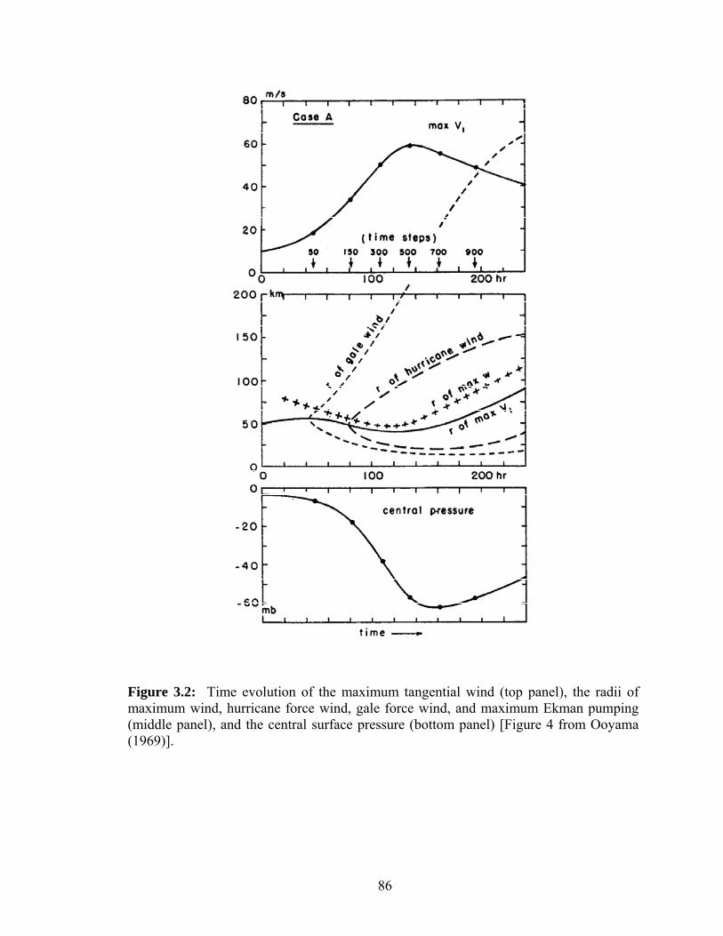
Figure 3.2: Time evolution of the maximum tangential wind (top panel), the radii of maximum wind, hurricane force wind, gale force wind, and maximum Ekman pumping (middle panel), and the central surface pressure (bottom panel) [Figure 4 from Ooyama (1969)].

86

Figure 3.3: Time evolution of the total kinetic energy for regions within radii of 100, 200, 500, and 1000 km [Figure 10 from Ooyama (1969)].

87

Figure 3.4: Time evolution of the vortex represented in Figures 3.2 and 3.3, displayed in K-Vmax space. The incipient, deepening, and mature stages are indicated respectively by green, red, and blue; with time marks every 12 hr. Labels across the top of the figure stand for tropical depression (TD), tropical storm (TS), and the five Saffir-Simpson hurricane categories (Cat 1-5). Excursions off this typical lifecycle can be caused by potential vorticity mixing and concentric eyewall cycles (the latter of which is shown schematically by the dashed blue line as a sudden decrease in Vmax as the inner eyewall dies). Three variations of the typical lifecycle time evolution are sometimes observed: small, intense storms labeled here as “Strong Dwarfs;” large, intense storms labeled here as “Super Giants;” and large, weak storms that are not of hurricane intensity, labeled here as “Weak Giants.”

88

Figure 3.5: K-Vmax scatterplot. Vmax and K determined from aircraft reconnaissance flight-level winds (700 mb). Dashed curve is ~ ; solid curve is best fit to K-Vmax data,

[Figure 2 from Maclay et al. (2008)]. ( ) 872.1max

1310*3 VK M =

89

Figure 3.6: Time evolution of K’-Vmax for six selected storms. K’ is the deviation of the observed K from ( ) 872.1

max1310*3 VK M = [Figure 4 from Maclay et al. (2008)].

90

Figure 3.7: Vertical structure functions appearing in (3.13) and (3.14). The blue curve is ( )[ ] ( TzzHz )πsin2exp , the vertical structure function in (3.13) corresponding to

, , and . The red curve is the vertical structure function in (3.14), ( )zrQ , ( zrTt ,( )

) ( )zrw ,[ ] ( ) [ ]( ) ( )[ ]TzzHzzz TT zH π π πsin22exp −cos , corresponding to ( )zrt ,φ , ( )zrvt , ,

and . ( )zru ,

91

Figure 3.8: Radial profiles of diabatic heating ( ) pcrQ̂ for the cases highlighted in Table 3.1. DH3 is shown in blue, DH5 in red, DH7 in green, DH9 in orange, DH11 in purple, and DH13 in cyan.

92

a)

b)

c)

Figure 3.9: Radial profiles of initial vortex a) tangential wind ( )rv , b) relative vorticity ( )rζ , and c) Rossby length ( )rl for Gaussian vortex R3V3 highlighted in Table 3.2.

93

a) b)

c) d)

e) f)

94

Figure 3.10: Changes in vortex structure for case DH3, where diabatic heating is constrained to occur inside the RMW. a) Initial radial profiles of diabatic heating ( )rQ̂ (grey background, scaled to maximum tangential wind), tangential wind (blue) and relative vorticity

( )rv( )rζ (red). b) Radial profile of secondary circulation: radial wind

(blue) and vertical velocity (red). c) Radial profile of temperature tendency in K day-1. d) Changes in tangential winds, with initial tangential winds (blue), tangential wind tendency (red), and surface tangential winds after six hours (green), as well as location of diabatic heating (grey). e) Radial profile of geopotential tendency

in m2s-2 day-1. f) Changes in relative vorticity, with initial relative vorticity

( )rv( )rvtˆ

( )rζ (blue), vorticity tendency ( )rtζ̂ (red), and surface relative vorticity after six hours (green), as well as location of diabatic heating (grey).

95

a) b)

c) d)

e) f)

Figure 3.11: Same as shown in Figure 3.10 for case DH5, where the heating profile is centered on the RMW.

96

a) b)

c) d)

e) f)

Figure 3.12: Same as shown in Figure 3.10 for case DH7, where the heating is inside the vorticity skirt region, just outside the RMW.

97

a) b)

c) d)

e) f)

Figure 3.13: Same as shown in Figure 3.10 for case DH9, where the heating is still almost entirely contained within the vorticity skirt region.

98

a) b)

c) d)

e) f)

Figure 3.14: Same as shown in Figure 3.10 for case DH11, where the heating is almost entirely outside the vorticity skirt region.

99

a) b)

c) d)

e) f)

Figure 3.15: Same as shown in Figure 3.10 for case DH13, where the heating is outside the vorticity skirt region.

100

Chapter 4

SUMMARY

4.1 Discussion

This dissertation focuses on the relationships found between tropical cyclone (TC)

structure and intensity – in particular between the TC eye and intensity trends. Chapters

2 and 3 investigated aspects of this relationship through observational and theoretical

modeling perspectives. This chapter ties the two projects together and outlines areas for

future progress in each project separately and in a combined framework.

TC intensity is dependent on large-scale environment, the storm-scale dynamics,

and the underlying ocean state (Kaplan et al. 2010). This combination of factors results

in an increase in the difficulty of forecasting TC intensity relative to TC track, which is to

first order dependent on the large-scale environment. Forecasts of TC track have

improved over the last few decades at a rate of approximately 1-2% per year, while

forecasts of TC intensity have seen little improvement over the past few decades

(Franklin et al. 2003, McAdie and Lawrence 2000, Rappaport et al. 2009). Intensity

forecasting, particularly for rapid intensity change, is viewed as a top priority for TC

research (Rappaport et al. 2009).

While global and regional dynamical models produce the most skillful TC track

forecasts, TC intensity is still forecast most accurately by statistical models, notably

101

SHIPS (Statistical Hurricane Intensity Prediction Scheme, DeMaria et al. 2005) and

LGEM (Logistic Growth Equation Model, DeMaria 2009). These models are less skillful

during periods of rapid intensity change, leading to the development of the RII (Rapid

Intensification Index, Kaplan et al. 2010). These statistical models forecast intensity

based on the large-scale environment and the underlying ocean state, and have started to

incorporate storm-scale dynamics using satellite-derived estimates of convection.

This dissertation focused on aspects of the effects of storm-scale dynamics on TC

intensity in two separate projects. The first project, discussed in Chapter 2, examined

observed eye structure in relation to intensity and intensity trend. To examine eye

structure a twenty year dataset of aircraft reconnaissance fixes from Atlantic basin TCs

was used, in combination with best track information on intensity, lifecycle and location.

Research into TC eye structures and processes has indicated that there are patterns

affecting both the TC eye and intensity. Concentric eyewall cycles, annular hurricanes,

and polygonal eyewalls can all influence intensity change (Willoughby et al. 1982,

Schubert et al. 1999, Knaff et al. 2003). Simple theoretical models show that contracting

eyewalls intensify (Shapiro and Willoughby 1982). However, this relationship between

contraction and intensification does not translate into a monotonic relationship between

eye diameter and intensity. Examination of aircraft reconnaissance in the northern West

Pacific basin has shown that no monotonic relationship is evident between eye diameter

and intensity (Jordan 1961, Weatherford 1989), though the most intense TCs all have

small eye diameters.

Chapter 2 focused on aircraft reconnaissance estimates of eye diameter and type

and their relationship to TC intensity and intensity change. Over the period 1989-2008,

102

aircraft reconnaissance was reported for 208 Atlantic TCs, with 109 TCs having at least

one eye estimate from the reconnaissance. Eyes were observed at all intensity categories,

from minimal tropical storms to category 5 hurricanes. Reconnaissance fixes that did not

report an eye estimate were limited to lower intensity TCs, rarely above category 1 in

intensity.

Eye diameter and intensity did not display a monotonic relationship, consistent

with previous studies (Jordan 1961, Weatherford 1989, Kimball and Mulekar 2004). The

median eye diameter for all estimates was 20 nmi, with smaller eye diameters for the TCs

with the lowest and highest intensities (tropical storms and category 5 hurricanes), and

larger eye diameters for mid-range intensities (category 2 and 3 hurricanes). Small eye

diameters were observed at all intensities, but large eye diameters were observed in a

more limited range. Large eye diameters were not observed in the most intense TCs,

consistent with Jordan (1961).

The median intensity change in six hours for all eye diameters was to maintain

intensity, though for eye diameters under 40 nmi more cases increased intensity than

decreased intensity. Eye diameters over 40 nmi had more cases decrease intensity than

increase intensity. Large eye diameters showed a tendency to maintain intensity or

decrease intensity slightly, consistent with behavior expected from annular hurricanes

(Knaff et al. 2003, Knaff et al. 2008). Small eye diameters, as well as having the largest

range in current intensity, also had the largest range in intensity change. Small eye

diameters had potentially large six hour changes in intensity both in the positive and

negative direction. This relationship held when examining intensity changes up to 24 hrs

after the eye estimate, indicating that knowledge of the eye size could improve

103

forecasting of rapid intensity change. Setting a rapid intensification threshold of 30 kt in

24 hrs (Kaplan et al. 2010), best track times with aircraft estimated eyes were associated

with a higher probability of past or current rapid intensification events than the general

best track sample.

Aircraft reconnaissance estimates of eye type were limited to three categories:

circular, elliptical, and concentric. The examination of eye type does not take into

account eye types with no corresponding option available like polygonal eyewalls

(Schubert et al. 1999, Kossin et al. 2002). Combinations of existing eye types could also

not be recorded, for example Hurricane Ivan (2004), during a concentric eyewall cycle on

12 September, displayed an outer eyewall that was elliptical (Hendricks et al. 2010). Eye

estimates were reported as circular in 80% of the cases, with elliptical comprising 15% of

the cases and concentric the remaining 5% of the cases. Both circular and elliptical eyes

were reported over the entire range of intensity. Concentric eyes were only observed in

hurricanes, consistent with satellite studies of concentric eyewalls (Kossin and Sitkowski

2009). Both circular and elliptical eyes were also reported at a wide range of eye

diameters, with a narrower range and smaller median eye diameter for concentric eyes.

Fewer than half the concentric eye cases had both inner and outer eye diameters reported.

Concentric eyes were most often reported directly following the maximum lifetime

intensity, though some TCs had concentric eyes at other points in their lifecycle or

multiple concentric eyewall cycles. Elliptical eyes were observed throughout the TC

lifecycle and at all intensities, in contrast to the earlier studies of northern West Pacific

TCs (Jordan 1961, Weatherford 1989).

104

Maps of the eye diameters provided by aircraft reconnaissance indicated some

influence on eye diameter based on the location and time of season. Smaller eye

diameters were observed at lower latitudes, consistent with theory that suggests the

minimum eye diameter for a given intensity increases as latitude increases due to

increased environmental angular momentum. Differences in eye diameters in the same

regions at different points of the season indicate a potential effect from differing

precursors or large-scale environment. These effects could be further investigated by

combining the environmental parameter dataset from SHIPS (DeMaria et al. 2005) with

the current dataset. The SHIPS parameters would allow for an examination of the large-

scale environment and ocean state for each system, and identify systematic differences

between TCs in similar locations at different points in the season. Vertical wind shear,

proximity to land, sea surface temperature, and ocean heat content in particular could all

play a role in identifying TCs that form eyes early and proceed to intensify versus those

that fail to intensify.

Another dataset that could provide useful additional information and cross-

referencing of the aircraft reconnaissance eye estimates would be the hurricane satellite

(HURSAT) dataset (Knapp and Kossin 2007, Kossin et al. 2007a,b). HURSAT would

help fill in the gaps left due to the limited aircraft availability, and comparisons of eye

diameters from the aircraft and HURSAT could be used to assist in identifying the

differences in the extended best track eye diameters (Demuth et al. 2006) from aircraft

estimates. Combining the two datasets also allows for examination of cases like the one

shown in Figures 4.1-4.2, in which Hurricane Wilma (2005, Beven et al. 2008) has an

aircraft-indicated eye diameter of 10 nmi or less at both times, but a satellite-indicated

105

eye at only the latter time. The assessment of satellite eye estimates would also allow for

the development of predictive tools that could function in the absence of aircraft

reconnaissance.

Chapter 3 focused on the relationship between the vortex structure and diabatic

heating in terms of the induced tangential wind tendencies using the balanced vortex

model (Eliassen 1952). The location of heating relative to an idealized axisymmetric

vorticity profile was varied, and the results described based on the heating location

relative to the radius of maximum winds (RMW) and the vorticity skirt. The results were

extremely sensitive to the placement of the diabatic heating relative to the vortex profile.

Any heating within the RMW produced a sharp increase in intensity. Heating within the

vorticity skirt also acted to intensify the vortex, though less than heating within the

RMW, while heating outside the vorticity skirt did not act to intensify the vortex.

The integrated kinetic energy (IKE) was also calculated and its change assessed

based on the placement of the heating. The IKE increased in all cases, but the efficiency

of the vortex in converting the heating to kinetic energy was increased in the high inertial

stability region within the RMW. Relative to the initial intensity and initial IKE,

intensity increased more than IKE for cases with heating within the RMW, both showed

approximately equal relative increases for cases of heating within the vorticity skirt, and

IKE increased more than intensity for cases of heating outside the vorticity skirt.

The idealized profiles used in this study can be extended in the framework

provided to more complex representations of an axisymmetric vortex and heating. One

approach is to use profiles generated by dynamical models to initialize our system, like

the profile shown from the Hurricane-Weather Research and Forecasting model (HWRF)

106

in Figure 4.3. The intensification and structure of the vortex from our model can be

compared with the forecast changes in the dynamical models. A second approach is to

use observations from a combination of aircraft reconnaissance and satellites to produce

the necessary initial profiles, and compare with observed changes in intensity.

The research from Chapters 2 and 3 can also be combined in the development of a

predictive tool for TC intensity change. The flight-level winds available from the aircraft

reconnaissance can be used to supply the initial vortex profile for the balanced vortex

model, but also to calculate the inner core wind radii, particularly the RMW for

comparison with the aircraft eye diameter estimates. Kimball and Mulekar (2004) found

that the distance between the eye radius and the RMW decreased as the intensity category

increased, but only looked in an average sense. The distance between the edge of the eye

and the RMW may serve as a useful proxy for the amount of heating contained within the

RMW and provide information on intensity change based on the vortex structure. The

eye diameter itself, while not directly correlated with intensity, could help provide error

bounds on the range of both current intensity and the possible rate of intensity change;

expanding from a more deterministic to probabilistic view.

107

Figure 4.1: Visible satellite image from GOES-12 (1 km resolution) of Hurricane Wilma at 1445 UTC 18 October. Wilma has already begun rapid intensification; the NHC best track data from 1200 UTC 18 October had maximum sustained winds of 65 kt and minimum sea level pressure of 979 hPa. A blow up of convection can be seen near the center of circulation. (Satellite image courtesy of Naval Research Lab website, http://www.nrlmry.navy.mil/sat_products.html)

108

Figure 4.2: Visible satellite image from GOES-10 (1 km resolution) of Hurricane Wilma at 1200 UTC 19 October. Wilma is at peak intensity, with maximum sustained winds of 160 kts and minimum sea level pressure of 882 mb (the lowest on record in the Atlantic basin). The eye diameter is 2 nmi. (Satellite image courtesy of Naval Research Lab website, http://www.nrlmry.navy.mil/sat_products.html)

109

Figure 4.3: Example of vortex and heating profiles calculated from HWRF fields. Azimuthally averaged 700 hPa winds (kt) in blue, vorticity (0.5*10-4 s-1) in red, and heating rate (K/hr) in grey shading.

110

REFERENCES

Abarca, S. F., and K. L. Corbosiero, 2011: Secondary eyewall formation in WRF simulations of Hurricanes Rita and Katrina (2005). Geophys. Res. Lett., 38, L07802, doi:10.1029/2011GL047015.

AMS Council, 2007: Hurricane forecasting in the United States: An information statement of the American Meteorological Society. Bull. Amer. Meteor. Soc., 88.

Arakawa, H., 1952: Mame-taifu or midget typhoon. Geophys. Mag., 23, 463-474.

ATCF Tropical Cyclone Database. http://www.nrlmry.navy.mil/atcf_web/docs/database/new/database.html, visited May 2007.

Beven, J. L., and Coauthors, 2008: Atlantic hurricane season of 2005. Mon. Wea. Rev., 136, 1109-1173.

Black, M. L., and H. E. Willoughby, 1992: The concentric eyewall cycle of Hurricane Gilbert. Mon. Wea. Rev., 120, 947-957.

Brand, S., 1972: Very large and very small typhoons of the western North Pacific Ocean. J. Meteor. Soc. Japan, 50, 332-341.

Cocks, S. B., and W. M. Gray, 2002: Variability of the outer wind profiles of western North Pacific typhoons: Classifications and techniques for analysis and forecasting. Mon. Wea. Rev., 130, 1989-2005.

Croxford, M., and G. M. Barnes, 2002: Inner core strength of Atlantic tropical cyclones. Mon. Wea. Rev., 130, 127-139.

111

Dean, L., K.A. Emanuel, and D. R. Chavas, 2009: On the size distribution of Atlantic tropical cyclones. Geophys. Res. Lett., 36, L14803, doi:10.1029/2009GL039051.

DeMaria, M., 2009: A simplified dynamical system for tropical cyclone intensity prediction. Mon. Wea. Rev., 137, 68-82.

DeMaria, M., M. Mainelli, L. K. Shay, J. A. Knaff, and J. Kaplan, 2005: Further improvements to the Statistical Hurricane Intensity Prediction Scheme (SHIPS). Wea. Forecasting, 20, 531-543.

Demuth, J., M. DeMaria, and J. A. Knaff, 2006: Improvement of advanced microwave sounder unit tropical cyclone intensity and size estimation algorithms. J. Appl. Meteor., 45, 1573-1581.

Dunn, G. E., and B. I. Miller, 1960: Atlantic Hurricanes. Louisiana State University Press, 326 pp.

Dunnavan, G. M., and J. W. Diercks, 1980: An analysis of Super Typhoon Tip (October 1979). Mon. Wea. Rev., 108, 1915-1923.

Eliassen, A., 1952: Slow thermally or frictionally controlled meridional circulation in a circular vortex. Astrophys. Norv., 5, 19-60.

Elsberry, R. L., and R. A. Stenger, 2008: Advances in understanding of tropical cyclone wind structure changes. Asia-Pac. J. Atmos. Sci., 44, 11-24.

Emanuel, K. A., 2000: A statistical analysis of tropical cyclone intensity. Mon. Wea. Rev., 128, 1139-1152.

Frank, W. M., 1977: The structure and energetic of the tropical cyclone I. Storm structure. Mon. Wea. Rev., 105, 1119-1135.

Franklin, J. L., cited 2009: National Hurricane Center forecast verification. [Available online at http://www.nhc.noaa.gov/verification.]

112

Franklin, J. L., C. J. McAdie, and M. B. Lawrence, 2003: Trends in track forecasting for tropical cyclones threatening the United States, 1970-2001. Bull. Amer. Meteor. Soc., 84, 1197-1203.

Franklin, J. L., and Coauthors, 2006: Atlantic hurricane season of 2004. Mon. Wea. Rev., 134, 981-1025.

Frederick, W. J., 2003: The rapid intensification and subsequent rapid weakening of Hurricane Lili as compared with historical hurricanes. Wea. Forecasting, 18, 1295-1298.

Hack, J. J., and W. H. Schubert, 1986: Nonlinear response of atmospheric vortices to heating by organized cumulus convection. J. Atmos. Sci., 43, 1559-1573.

Harr, P. A., M. S. Kalafsky, and R. L. Elsberry, 1996: Environmental conditions prior to formation of a midget tropical cyclone during TCM-93. Mon. Wea. Rev., 124, 1693-1710.

Hawkins, H. F., and D. T. Rubsam, 1967: Hurricane Inez – a classic “micro-hurricane.” Mar. Wea. Log, 11, 157-160.

Hawkins, H. F., and S. M. Imbembo, 1976: The structure of a small, intense hurricane – Inez 1966. Mon. Wea. Rev., 104, 418-442.

Hawkins, J. D., and Coauthors, 2006: Tropical cyclone multiple eyewall configurations. Extended Abstracts, 27th Conf. on Hurricanes and Tropical Meteorology, Monterey, CA, Amer. Met. Soc., 6B.1.

Hendricks, E. A., and W. H. Schubert, 2010: Adiabatic rearrangement of hollow PV towers. J. Adv. Model. Earth Syst., 2, 19 pp.

Hendricks, E. A., W. H. Schubert, R. K. Taft, H. Wang, and J. P. Kossin, 2009: Life cycles of hurricane-like vorticity rings. J. Atmos. Sci., 66, 705-722.

Hendricks, E. A., W. H. Schubert, S. R. Fulton, and B. D. McNoldy, 2010: Spontaneous-adjustment emission of inertia-gravity waves by unsteady vertical motion in the hurricane core. Q. J. R. Meteorol. Soc., 136, 537-548.

113

Hill, K. A., and G. M. Lackmann, 2009: Influence of environmental humidity on tropical cyclone size. Mon. Wea. Rev., 137, 3294-3315.

Holliday, C. R., 1973: Record 12- and 24-hour deepening rates in a tropical cyclone. Mon. Wea. Rev., 101, 112-114.

Holliday, C. R., and A. H. Thompson, 1979: Climatological characteristics of rapidly intensifying typhoons. Mon. Wea. Rev., 107, 1022-1034.

Houze, R. A., Jr., S. S. Chen, B. F. Smull, W.-C. Lee, and M. M. Bell, 2007: Hurricane intensity and eyewall replacement. Science, 315, 1235-1239.

Jordan, C. L., 1961: Marked changes in the characteristics of the eye of intense typhoons between the deepening and filling stages. J. Meteor., 18, 779-789.

Jordan, C. L., and F. J. Schatzle, 1961: The “double eye” of Hurricane Donna. Mon. Wea. Rev., 89, 354-356.

Kantha, L., 2006: Time to replace the Saffir-Simpson hurricane scale? Eos, Trans. Amer. Geophys. Union, 87, 3-6.

Kaplan, J., and M. DeMaria, 2003: Large-scale characteristics of rapidly intensifying tropical cyclones in the North Atlantic basin. Wea. Forecasting, 18, 1093-1108.

Kaplan, J., M. DeMaria, and J. A. Knaff, 2010: A revised tropical cyclone rapid intensification index for the Atlantic and Eastern North Pacific basins. Wea. Forecasting, 25, 220-241.

Kimball, S. K., and M. S. Mulekar, 2004: A 15-year climatology of North Atlantic tropical cyclones. Part I: Size parameters. J. Climate, 17, 3555-3575.

Knaff, J. A., J. P. Kossin, and M. DeMaria, 2003: Annular hurricanes. Wea. Forecasting, 18, 204-222.

114

Knaff, J. A., T. A. Cram, A. B. Schumacher, J. P. Kossin, and M. DeMaria, 2008: Objective identification of annular hurricanes. Wea. Forecasting, 23, 17-28.

Knapp, K. R., and J. P. Kossin, 2007: A new global tropical cyclone dataset from ISCCP B1 geostationary satellite observations. J. Appl. Remote Sensing, 1, 013505, doi:10.1117/12.731296.

Kossin, J. P., and M. D. Eastin, 2001: Two distinct regimes in the kinematic and thermodynamic structure of the hurricane eye and eyewall. J. Atmos. Sci., 58, 1079-1090.

Kossin, J. P., and M. Sitkowski, 2009: An objective model for identifying secondary eyewall formation in hurricanes. Mon. Wea. Rev., 137, 876-892.

Kossin, J. P., W. H. Schubert, and M. T. Montgomery, 2000: Unstable interactions between a hurricane’s primary eyewall and a secondary ring of enhanced vorticity. J. Atmos. Sci., 57, 3893-3917.

Kossin, J. P., B. D. McNoldy, and W. H. Schubert, 2002: Vortical swirls in hurricane eye clouds. Mon. Wea. Rev., 130, 3144-3149.

Kossin, J. P., K. R. Knapp, D. J. Vimont, R. J. Murnane, and B. A. Harper, 2007a: A globally consistent reanalysis of hurricane variability and trends. Geophys. Res. Lett., 34, L04815, doi:10.1029/2006GL028836.

Kossin, J. P., and Coauthors, 2007b: Estimating hurricane wind structure in the absence of aircraft reconnaissance. Wea. Forecasting, 22, 89-101.

Kuo, H.-C., L.-Y. Lin, C.-P. Chang, and R. T. Williams, 2004: The formation of concentric vorticity structures in typhoons. J. Atmos. Sci., 61, 2722-2734.

Kuo, H.-C., W. H. Schubert, C.-L. Tsai, and Y.-F. Kuo, 2008: Vortex interactions and barotropic aspects of concentric eyewall formation. Mon. Wea. Rev., 136, 5183-5198.

Kuo, H. L., 1959: Dynamics of convective vortices and eye formation. The Atmosphere and Sea in Motion, B. Bolin, Ed., Rockefeller Inst. Press, 413-424

115

Lander, M. A., 1999: A tropical cyclone with a very large eye. Mon. Wea. Rev., 127, 137-142.

Maclay, K. S., M. DeMaria, and T. H. Vonder Haar, 2008: Tropical cyclone inner-core kinetic energy evolution. Mon. Wea. Rev., 136, 4882-4898.

Mallen, K. J., M. T. Montgomery, and B. Wang, 2005: Re-examining the near-core radial structure of the tropical cyclone primary circulation: Implications for vortex resiliency. J. Atmos. Sci., 62, 408-425.

McAdie, C. M., and M. B. Lawrence, 2000: Improvements in tropical cyclone track forecasting in the Atlantic basin, 1970-1998. Bul. Amer. Meteor. Soc., 81, 989-997.

McNoldy, B. D., 2004: Triple eyewalls in Hurricane Juliette. Bul. Amer. Meteor. Soc., 85, 1663-1666.

Merrill, R. T., 1984: A comparison of large and small tropical cyclones. Mon. Wea. Rev., 112, 1408-1418.

Miller, R. J., A. J. Schrader, C. R. Sampson, and T. L. Tsui, 1990: The Automated Tropical Cyclone Forecasting System (ATCF). Wea. Forecasting, 5, 653-660.

Ooyama, K., 1969: Numerical simulation of the life cycle of tropical cyclones. J. Atmos. Sci., 26, 3-40.

Powell, M. D., and T. A. Reinhold, 2007: Tropical cyclone destructive potential by integrated kinetic energy. Bull. Amer. Meteor. Soc., 88, 513-526.

Rappaport, E. N., and Coauthors, 2009: Advances and challenges at the National Hurricane Center. Wea. Forecasting, 24, 395-419.

Riehl, H., 1979: Climate and Weather in the Tropics. Academic Press, 611 pp.

Rozoff, C. M., W. H. Schubert, and J. P. Kossin, 2008: Some dynamical aspects of tropical cyclone concentric eyewalls. Q. J. R. Meteorol. Soc., 134, 583-593.

116

Sampson, C. R., and A. J. Schrader, 2000: The Automated Tropical Cyclone Forecasting System (Version 3.2). Bull. Amer. Meteor. Soc., 81, 1231-1240.

Schubert, W. H., and J. J. Hack, 1982: Inertial stability and tropical cyclone development. J. Atmos. Sci., 39, 1687-1697.

Schubert, W. H., M. T. Montgomery, R. K. Taft, T. A. Guinn, S. R. Fulton, J. P. Kossin, and J. P. Edwards, 1999: Polygonal eyewalls, asymmetric eye contraction, and potential vorticity mixing in hurricanes. J. Atmos. Sci., 56, 1197-1223.

Shapiro, L. J., and H. E. Willoughby, 1982: The response of balanced hurricanes to local sources of heat and momentum. J. Atmos. Sci., 39, 378-394.

Shen, W., 2006: Does the size of hurricane eye matter with its intensity? Geophys. Res. Lett., 33, L18813, doi:10.1029/2006GL027313.

Simpson, R. H., and H. Riehl, 1981: The Hurricane and Its Impact. Louisiana State University Press, 398 pp.

Simpson, R. H., and H. Saffir, 2007: Comments on “Tropical cyclone destructive potential by integrated kinetic energy.” Bull. Amer. Meteor. Soc., 88, 1799-1800.

Terwey, W. D., and M. T. Montgomery, 2008: Secondary eyewall formation in two idealized, full-physics modeled hurricanes. J. Geophys. Res., 113, D12112, doi:10.1029/2007JD008897.

Vigh, J. L., and W. H. Schubert, 2009: Rapid development of the tropical cyclone warm core. J. Atmos. Sci., 66, 3335-3350.

Wang, Y., 2008: Structure and formation of an annular hurricane simulated in a fully compressible, nonhydrostatic model – TCM4. J. Atmos. Sci., 65, 1505-1527.

Weatherford, C. L., 1989: The structural evolution of typhoons. Atm. Sci. Paper 446, Colorado State University, 198 pp.

117

118

Weatherford, C. L., and W. M. Gray, 1988a: Typhoon structure as revealed by aircraft reconnaissance. Part I: Data analysis and climatology. Mon. Wea. Rev., 116, 1032-1043.

Weatherford, C. L., and W. M. Gray, 1988b: Typhoon structure as revealed by aircraft reconnaissance. Part II: Structural variability. Mon. Wea. Rev., 116, 1044-1056.

Willoughby, H. E., J.A. Clos, and M. G. Shoreibah, 1982: Concentric eyewalls, secondary wind maxima, and the evolution of the hurricane vortex. J. Atmos. Sci., 39, 395-411.

Zhang, Q.-H., S.-J. Chen, Y.-H. Kuo, K.-H. Lau, and R. A. Anthes, 2005: Numerical study of a typhoon with a large eye: Model simulation and verification. Mon. Wea. Rev., 133, 725-742.

Zhou, X., and B. Wang, 2009: From concentric eyewall to annular hurricane: A numerical study with the cloud-resolved WRF model. Geophys. Res. Lett., 36, L03802, doi:10.1029/2008GL036854.