Discrete Convex Analysis - University of...

Discrete Convex Analysis

Kazuo Murota∗

January 1996 (Revision: October 1997)

Mathematical Programming No. P-1196, Revised Version

Abstract

A theory of “discrete convex analysis” is developed for integer-valuedfunctions defined on integer lattice points. The theory parallels the ordi-nary convex analysis, covering discrete analogues of the fundamental con-cepts such as conjugacy, subgradients, the Fenchel min-max duality, sepa-ration theorems and the Lagrange duality framework for convex/nonconvexoptimization. The technical development is based on matroid-theoretic con-cepts, in particular, submodular functions and exchange axioms. Part Iextends the conjugacy relationship between submodularity and exchange-ability, deepening our understanding of the relationship between convexityand submodularity investigated in the eighties by A. Frank, S. Fujishige,L. Lovasz and others. Part II establishes duality theorems for M- andL-convex functions, namely, the Fenchel min-max duality and separationtheorems. These are the generalizations of the discrete separation theo-rem for submodular functions due to A. Frank and the optimality criteriafor the submodular flow problem due to M. Iri–N. Tomizawa, S. Fujishige,and A. Frank. A novel Lagrange duality framework is also developed ininteger programming. We follow Rockafellar’s conjugate duality approachto convex/nonconvex programs in nonlinear optimization, while technicallyrelying on the fundamental theorems of matroid-theoretic nature.

Keywords: convex analysis, combinatorial optimization, discrete separation

theorem, integer programming, Lagrange duality, submodular function

AMS Classifications: 90C27; 90C25, 90C10, 90C35.

Address for correspondence:Kazuo Murota

Research Institute for Mathematical Sciences

Kyoto University, Kyoto 606-01, Japan

facsimile: +81-75-753-7272 , e-mail: [email protected]

∗Research Institute for Mathematical Sciences, Kyoto University, Kyoto 606-01, Japan, e-mail: [email protected],

1

Part I: Conjugacy

1 Introduction

In the field of nonlinear programming (in continuous variables) the generalized La-

grange duality plays a pivotal role both in theory and in practice. The perturbation-

based duality scheme, developed primarily by R. T. Rockafellar [43], [44], is based

on the concept of conjugate duality for convex functions. The objective of this pa-

per is to develop an analogous theory for discrete optimization (nonlinear integer

programming) by combining and generalizing the ideas in convex analysis and the

results in matroid theory. This amounts to developing a theory that may be called

“discrete convex analysis.” To be specific, we give a Lagrange duality scheme for

the following optimization problem:

Minimize f(x) subject to x ∈ B, (1.1)

where f : Zn → Z ∪ {+∞} and B ⊆ Zn.

To motivate our framework involving matroid-theoretic concepts, let us first

introduce a naive approach (without matroidal structure) and discuss its short-

comings. For B ⊆ Zn it seems natural to regard B as a “convex set” (discrete

analogue of a convex set) if B = Zn ∩B holds, where B denotes the convex hull of

B. Likewise, for f : Zn → Z∪ {+∞} it seems natural to define f to be a “convex

function” if it can be extended to a convex function in the usual sense, namely,

there exists a convex function f : Rn → R ∪ {+∞} such that f(x) = f(x) for

x ∈ Zn and domRf = domZf , where

domRf = {x ∈ Rn | f(x) is finite},

domZf = {x ∈ Zn | f(x) is finite}.

We can proceed further to imitate the construction in convex analysis [43], [49] by

replacing R to Z in the defining formulas such as

h∗(p) = sup{〈p, x〉 − h(x) | x ∈ Rn} (p ∈ Rn) (1.2)

for the (convex) conjugate function (the Fenchel transform) of h : Rn → R∪{+∞}and

∂h(x) = ∂Rh(x) = {p ∈ Rn | h(x′) − h(x) ≥ 〈p, x′ − x〉 (∀x′ ∈ Rn)} (1.3)

for the subdifferential. To be specific, we can define the “conjugate function” (the

“integer Fenchel transform”) f• : Zn → Z ∪ {+∞} of f : Zn → Z ∪ {+∞} by

f•(p) = sup{〈p, x〉 − f(x) | x ∈ Zn} (p ∈ Zn), (1.4)

2

where domZf is assumed to be nonempty, and the “integer subdifferential” by

∂Zf(x) = {p ∈ Zn | f(x′) − f(x) ≥ 〈p, x′ − x〉 (∀x′ ∈ Zn)}. (1.5)

Unfortunately, these definitions fail to yield an interesting theory. This is

mainly because of the lack of duality theorems (separation theorem, Fenchel’s

min-max theorem, etc.), which lie at the very heart of the convex analysis. It

should be clear in this connection that the fundamental formulas in the convex

analysis such as h∗∗ = h and ∂R(h1 + h2) = ∂Rh1 + ∂Rh2 rely on the duality

theorems. The following examples demonstrate the failure of such identities in the

discrete case and hence limitations of this model for “discrete convex analysis.”

Example 1.1 [f•• 6= f , ∂Zf(0) = ∅] Let f : Z3 → Z ∪ {+∞} be defined by

domZf = {(0, 0, 0),±(1, 1, 0),±(0, 1, 1),±(1, 0, 1)},

f(0, 0, 0) = 0, f(1, 1, 0) = f(0, 1, 1) = f(1, 0, 1) = 1,

f(−1,−1, 0) = f(0,−1,−1) = f(−1, 0,−1) = −1.

This function can be extended to a convex function f : R3 → R ∪ {+∞} with

domRf = domZf . In fact, domZf is a “convex set” in the sense that domZf =

ZV ∩ domZf , and f is given by

f(x1, x2, x3) =

{(x1 + x2 + x3)/2 (x ∈ domZf)

+∞ (x 6∈ domZf)

The “conjugate function” f• : Z3 → Z ∪ {+∞} of f , as defined in (1.4), is given

by

f•(p) = supx∈Z3

(〈p, x〉 − f(x))

= max(0, |p1 + p2 − 1|, |p2 + p3 − 1|, |p3 + p1 − 1|).

The “biconjugate function”, based on (1.4), is given by

f••(x) = supp∈Z3

(〈p, x〉 − f•(p))

= supp∈Z3

(〈p, x〉 − max(0, |p1 + p2 − 1|, |p2 + p3 − 1|, |p3 + p1 − 1|)).

Hence we have f••(0) = −1 6= 0 = f(0). On the other hand,

f∗∗

(0) = supp∈R3

(〈p, 0〉 − f∗(p))

= supp∈R3

(−max(0, |p1 + p2 − 1|, |p2 + p3 − 1|, |p3 + p1 − 1|))

= 0 = f(0)

3

with the supremum attained by p =(

12, 1

2, 1

2

). The subdifferential of f at x = 0 is

given by

∂Rf(0) = {p ∈ R3 | f(x′) − f(0) ≥ 〈p, x′〉 (∀x′ ∈ R3)} ={(

1

2,1

2,1

2

)},

whereas ∂Zf(0) = ∅. The phenomena, f•• 6= f and ∂Zf(0) = ∅, demonstrated

here are certainly undesirable. 2

Example 1.2 [∂Z(f1 + f2) 6= ∂Zf1 + ∂Zf2] Consider f1, f2 : Z2 → Z defined by

f1(x1, x2) = max(0, x1 + x2), f2(x1, x2) = −min(x1, x2),

which can be extended naturally to f1, f2 : R2 → R according to their expressions.

We have

∂Zf1(0) = {(0, 0), (1, 1)}, ∂Zf2(0) = {(−1, 0), (0,−1)},

from which follows

∂Zf1(0) + ∂Zf2(0) = {±(1, 0),±(0, 1)}.

On the other hand, we have

(f1 + f2)(x) = max(|x1|, |x2|), ∂Z(f1 + f2)(0) = {(0, 0),±(1, 0),±(0, 1)}.

Hence ∂Z(f1 + f2)(0) 6= ∂Zf1(0) + ∂Zf2(0), which should be compared with

∂R(f1 + f2)(0) = ∂Rf1(0) + ∂Rf2(0) = convex hull of {±(1, 0),±(0, 1)}.

2

Example 1.3 [failure of discrete separation] Let B = {(x1, x2, x3) ∈ Z3 | x1 +

x2 + x3 = 0}, and define f : Z3 → Z ∪ {+∞} and g : Z3 → Z ∪ {−∞} by

f(x1, x2, x3) =

{max(0,−x3) ((x1, x2, x3) ∈ B)

+∞ ((x1, x2, x3) 6∈ B)

g(x1, x2, x3) =

{min(x1, x2) ((x1, x2, x3) ∈ B)

−∞ ((x1, x2, x3) 6∈ B)

Obviously, f and g can be extended respectively to a convex function f : R3 → R∪{+∞} and to a concave function g : R3 → R∪{−∞} with domRf = domRg = B.

It can be verified that f(x) ≥ g(x) for all x ∈ R3 and, by the separation theorem in

convex analysis, there exists p ∈ R3 such that f(x) ≥ 〈p, x〉 ≥ g(x) for all x ∈ R3.

In fact, we can take p =(

12, 1

2, 0

). However, there exists no integral vector p ∈ Z3

such that f(x) ≥ 〈p, x〉 ≥ g(x) for all x ∈ Z3, although f(x) ≥ 〈p, x〉 ≥ g(x) for all

x ∈ Z3 with p =(

12, 1

2, 0

). This demonstrates the failure of the desired discreteness

in the separation theorem. Note also that ∂Zf(x) 6= ∅ and ∂Z(−g)(x) 6= ∅ for

x ∈ B. 2

4

The above examples suggest that we must identify a more restrictive class of

well-behaved “convex functions” in order to develop a theory of “discrete convex

analysis.”

A clue is found in the theory of matroids and submodular functions, which has

successfully captured the combinatorial essence underlying the well-solved class of

combinatorial optimization problems such as those on graphs and networks (cf.,

Faigle [11], Fujishige [19], Lawler [30]). The relationship between convex functions

and submodular functions was made clear in the eighties through the works of

A. Frank, S. Fujishige, and L. Lovasz (see Section 3 for details). Fujishige [17],

[18] formulated Edmonds’ intersection theorem as a Fenchel-type min-max duality

theorem, with an integrality assertion in the case of integer-valued functions, and

considered further analogies such as subgradients. Frank [14] showed a separation

theorem for a pair of submodular/supermodular functions, with an integrality

assertion for the separating hyperplane in the case of integer-valued functions.

This theorem can also be regarded as being equivalent to Edmonds’ intersection

theorem. A precise statement, beyond analogy, about the relationship between

convex functions and submodular functions was made by Lovasz [31]. Namely, a

set function is submodular if and only if the so-called Lovasz extension of that

function is convex. This penetrating remark established a direct link between

the duality for convex/concave functions and that for submodular/supermodular

functions. The essence of the duality for submodular/supermodular functions is

now recognized as the discreteness (integrality) assertion in addition to the duality

for convex/concave functions.

In spite of the development in the eighties, our understanding of the relationship

between convexity and submodularity seems to be only partial in the sense that

it is restricted to the “convexity” of a (discrete) set and its support function.

Let V be a finite set and ρ : 2V → Z ∪ {+∞} be a submodular function

(ρ(X) + ρ(Y ) ≥ ρ(X ∪ Y ) + ρ(X ∩ Y ) for all X,Y ⊆ V ) such that ρ(∅) = 0 and

ρ(V ) is finite1 . It determines a set B ⊆ ZV by

B = {x ∈ ZV | supX⊆V

(〈χX , x〉 − ρ(X)) = 0; 〈χV , x〉 − ρ(V ) = 0}, (1.6)

where χX ∈ {0, 1}V is the characteristic vector of X ⊆ V (defined by χX(v) = 1 if

v ∈ X, and = 0 otherwise). As is well known, B enjoys the simultaneous exchange

property:

(B-EXC) For x, y ∈ B and for u ∈ supp+(x − y), there exists v ∈ supp−(x − y)

such that x − χu + χv ∈ B and y + χu − χv ∈ B,

1Namely, (dom ρ, ρ|dom ρ) is a submodular system in the sense of Fujishige [19], where dom ρ ={X ⊆ V | ρ(X) < +∞} and ρ|dom ρ is the restriction of ρ to dom ρ.

5

where

supp+(x − y) = {u ∈ V | x(u) > y(u)}, supp−(x − y) = {v ∈ V | x(v) < y(v)},

and χu = χ{u} denotes the characteristic vector of u ∈ V . We say B ⊆ ZV is an

integral base set if it satisfies (B-EXC). An integral base set B satisfies B = ZV ∩B

(being “convex”) and B will be called in this paper the integral base polyhedron

(which agrees with the base polyhedron of an integral submodular system; see

Section 3 for basic facts on submodular functions).

By the submodularity of ρ, its Lovasz extension ρ : RV → R ∪ {+∞} agrees

with the support function of B, i.e.,

ρ(p) = sup{〈p, x〉 | x ∈ B} = sup{〈p, x〉 | x ∈ B},

which implies in particular that ρ(p) = δB•(p) for p ∈ ZV (i.e., ρ|ZV = δB

•), where

δB : ZV → {0, +∞} is the indicator function of B (i.e., δB(x) = 0 if x ∈ B, and

= +∞ otherwise) and δB• is the “conjugate” of δB defined in (1.4). It is noted

that the equality ρ|ZV = δB• is essentially a duality (conjugacy) assertion, i.e.,

δB•• = δB, since the definition of B in (1.6) says in effect that δB = (ρ|ZV )•.

We also see that Frank’s discrete separation theorem asserts that two disjoint

integral base sets can be separated by a hyperplane defined in terms of {0,±1}-vectors (see Theorem 3.6). In this way, the duality results concerning submodular

functions are satisfactory enough for us to regard an integral base set as the discrete

analogue of a convex set. However, the duality concerning submodular functions

does not enjoy full generality from the viewpoint of “discrete convex analysis,” in

which a “convex function” is involved as the objective function in addition to a

“convex set” of feasible solutions.

A discrete analogue of “convex functions” has been identified very recently by

the present author (Murota [37], [38], [39]) as a natural extension of the concept

of valuated matroid introduced by Dress–Wenzel [7], [8]. In accordance with this,

we consider two “convexity” classes that are conjugate through the transformation

(1.4). To denote these two classes we coin two words, M-convexity and L-convexity,

for functions f : ZV → Z ∪ {+∞}.We define f : ZV → Z ∪ {+∞} to be M-convex if domZf 6= ∅ and it satisfies

the following quantitative generalization of the simultaneous exchange property:

(M-EXC) For x, y ∈ domZf and u ∈ supp+(x− y) there exists v ∈ supp−(x− y)

such that

f(x) + f(y) ≥ f(x − χu + χv) + f(y + χu − χv).

As will be explained later in Theorem 4.11, f : ZV → Z ∪ {+∞} is M-convex if

and only if it can be extended to a convex function f : RV → R ∪ {+∞} such

6

that, for each p ∈ RV ,

{x ∈ RV | f(x) − 〈p, x〉 ≤ f(x′) − 〈p, x′〉 (∀x′ ∈ RV )}

forms an integral base polyhedron. Hence the class of M-convex functions is a

subclass of the “convex functions” in the afore-defined sense based on the extend-

ability. Some instances of M-convex functions are listed in Section 2.

Naturally, we call g : ZV → Z ∪ {−∞} M-concave if −g is M-convex. An

M-concave function g with domZg ⊆ {0, 1}V can be identified with a valuated

matroid in the sense of Dress–Wenzel [7], [8]. A general M-concave function has

been employed by Murota [37] to generalize the cost function in the submodular

flow problem.

M-convexity plays the principal role in this paper. The objective function f of

the (primal) optimization problem (1.1) is often assumed to be M-convex, though

this is not an absolute prerequisite for the development of the Lagrange duality

scheme.

The other class, L-convex functions, consists of functions f : ZV → Z∪ {+∞}that are submodular on the vector lattice ZV and satisfy an additional condition

that

∃r ∈ Z,∀p ∈ ZV : f(p + 1) = f(p) + r,

where 1 = (1, 1, · · · , 1) ∈ ZV . It should be clear that submodularity on the vector

lattice ZV means

f(p) + f(q) ≥ f(p ∨ q) + f(p ∧ q) (p, q ∈ ZV )

with p∨q and p∧q denoting integral vectors defined by (p∨q)(v) = max(p(v), q(v))

and (p ∧ q)(v) = min(p(v), q(v)). It will be shown that L-convex functions can be

extended to convex functions on RV and moreover that they are nothing but those

functions which are conjugate to M-convex functions. The restriction to ZV of the

Lovasz extension of a submodular function ρ : 2V → Z∪{+∞} is an L-convex func-

tion. The L-convex functions turn out to constitute another class of well-behaved

“convex functions” that inherit the nice properties from submodular functions on

the boolean lattice 2V as well as from convex functions on RV . Naturally, we

call g : ZV → Z ∪ {−∞} L-concave if −g is L-convex. The Lagrange dual of

the optimization problem (1.1), to be defined in Section 6, will have an L-concave

objective function to be maximized.

This paper is organized as follows. Sections 2 to 5 establish the fundamental

theorems in “discrete convex analysis.” Section 2 provides a number of natural

classes of M-convex functions. Section 3 reviews relevant results on submodular

functions. Section 4 shows fundamental properties of M- and L-convex functions,

while Section 5 concentrates on duality theorems. Finally, Section 6 employs

7

the established theorems to develop a discrete analogue of the Lagrange duality

scheme for the optimization problem (1.1) by adapting Rockafellar’s conjugate

duality approach in nonlinear optimization. The “convex programs” correspond

to the case of (1.1) when f is an M-convex function and B is an integral base

set, whereas the duality scheme is capable of dealing with “nonconvex programs”

using a discrete analogue of the augmented Lagrangian.

8

2 Examples of M-convex Functions

We show a number of natural classes of M-convex functions.

Example 2.1 (Affine function) Let B ⊆ ZV be an integral base set that satis-

fies, by definition, the exchange property (B-EXC). For η : V → Z and α ∈ Z, the

function f : ZV → Z ∪ {+∞} defined by

f(x) = α + 〈η, x〉 (x ∈ B), domZf = B,

is M-convex, with equality in (M-EXC). This is an immediate consequence of (B-

EXC). 2

Example 2.2 (Separable convex function) Let B ⊆ ZV be an integral base

set. We call f0 : Z → Z ∪ {+∞} convex if its piecewise linear extension f0 :

R → R ∪ {+∞} is a convex function. For a family of convex functions fv : Z →Z∪{+∞} indexed by v ∈ V , the (separable convex) function f : ZV → Z∪{+∞}defined by

f(x) =∑

{fv(x(v)) | v ∈ V } (x ∈ B), domZf = B,

is M-convex. To see this, take x, y ∈ B and u ∈ supp+(x − y). By (B-EXC) there

exists v ∈ supp−(x − y) such that x′ ≡ x − χu + χv ∈ B, y′ ≡ y + χu − χv ∈ B.

Then we have

f(x′) + f(y′) = [fu(x(u) − 1) + fu(y(u) + 1)] + [fv(x(v) + 1) + fv(y(v) − 1)]

+∑

w 6=u,v

[fw(x(w)) + fw(y(w))].

By the convexity of fu and the relations y(u) ≤ x(u) − 1 ≤ x(u) and y(u) ≤y(u) + 1 ≤ x(u), we see that

fu(x(u) − 1) + fu(y(u) + 1) ≤ fu(x(u)) + fu(y(u)).

Similarly we have

fv(x(v) + 1) + fv(y(v) − 1) ≤ fv(x(v)) + fv(y(v)).

Hence we obtain f(x′) + f(y′) ≤ f(x) + f(y). The minimization problem of a

separable convex function on an integral base set has been considered by Fujishige

[19, Section 8]. 2

Example 2.3 (Min-cost flow) M-convexity is inherent in the integer minimum-

cost flow problem with a separable convex objective function, which has been

investigated by Minoux [32], Rockafellar [45] and others.

9

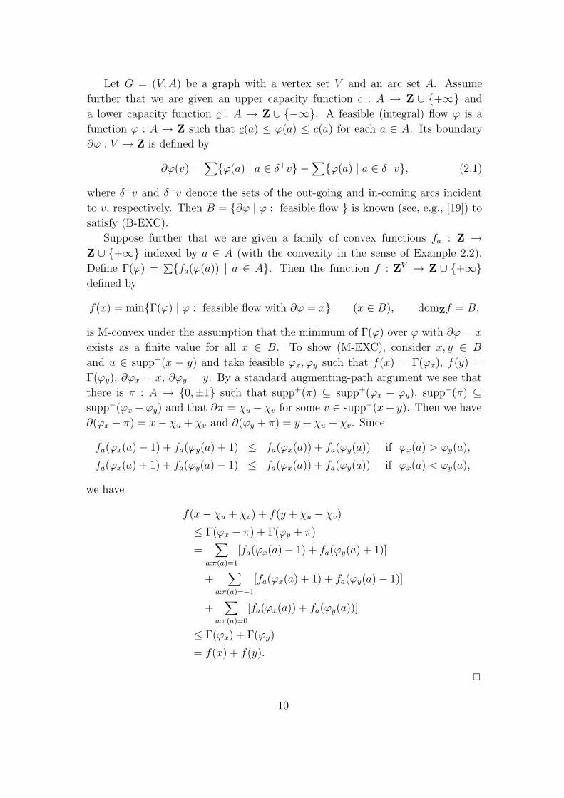
Let G = (V,A) be a graph with a vertex set V and an arc set A. Assume

further that we are given an upper capacity function c : A → Z ∪ {+∞} and

a lower capacity function c : A → Z ∪ {−∞}. A feasible (integral) flow ϕ is a

function ϕ : A → Z such that c(a) ≤ ϕ(a) ≤ c(a) for each a ∈ A. Its boundary

∂ϕ : V → Z is defined by

∂ϕ(v) =∑

{ϕ(a) | a ∈ δ+v} −∑

{ϕ(a) | a ∈ δ−v}, (2.1)

where δ+v and δ−v denote the sets of the out-going and in-coming arcs incident

to v, respectively. Then B = {∂ϕ | ϕ : feasible flow } is known (see, e.g., [19]) to

satisfy (B-EXC).

Suppose further that we are given a family of convex functions fa : Z →Z ∪ {+∞} indexed by a ∈ A (with the convexity in the sense of Example 2.2).

Define Γ(ϕ) =∑{fa(ϕ(a)) | a ∈ A}. Then the function f : ZV → Z ∪ {+∞}

defined by

f(x) = min{Γ(ϕ) | ϕ : feasible flow with ∂ϕ = x} (x ∈ B), domZf = B,

is M-convex under the assumption that the minimum of Γ(ϕ) over ϕ with ∂ϕ = x

exists as a finite value for all x ∈ B. To show (M-EXC), consider x, y ∈ B

and u ∈ supp+(x − y) and take feasible ϕx, ϕy such that f(x) = Γ(ϕx), f(y) =

Γ(ϕy), ∂ϕx = x, ∂ϕy = y. By a standard augmenting-path argument we see that

there is π : A → {0,±1} such that supp+(π) ⊆ supp+(ϕx − ϕy), supp−(π) ⊆supp−(ϕx −ϕy) and that ∂π = χu − χv for some v ∈ supp−(x− y). Then we have

∂(ϕx − π) = x − χu + χv and ∂(ϕy + π) = y + χu − χv. Since

fa(ϕx(a) − 1) + fa(ϕy(a) + 1) ≤ fa(ϕx(a)) + fa(ϕy(a)) if ϕx(a) > ϕy(a),

fa(ϕx(a) + 1) + fa(ϕy(a) − 1) ≤ fa(ϕx(a)) + fa(ϕy(a)) if ϕx(a) < ϕy(a),

we have

f(x − χu + χv) + f(y + χu − χv)

≤ Γ(ϕx − π) + Γ(ϕy + π)

=∑

a:π(a)=1

[fa(ϕx(a) − 1) + fa(ϕy(a) + 1)]

+∑

a:π(a)=−1

[fa(ϕx(a) + 1) + fa(ϕy(a) − 1)]

+∑

a:π(a)=0

[fa(ϕx(a)) + fa(ϕy(a))]

≤ Γ(ϕx) + Γ(ϕy)

= f(x) + f(y).

2

10

Example 2.4 (Determinant [7], [8]) Let A(t) be an m × n matrix of rank m

with each entry being a polynomial in a variable t, and let M = (V,B) denote the

(linear) matroid defined on the column set V of A(t) by the linear independence

of the column vectors, where J ⊆ V belongs to B if and only if |J | = m and the

column vectors with indices in J are linearly independent. Let B be the set of the

incidence vectors χJ of the bases J (the members of B), i.e., B = {χJ | J ∈ B}.Then f : ZV → Z ∪ {+∞} defined by

f(χJ) = − degt det A[J ] (J ∈ B), domZf = B,

is M-convex, where A[J ] denotes the m×m submatrix with column indices in J . In

fact the Grassmann-Plucker identity implies the exchange property of f and this

example was the motivation for introduction of the concept of valuated matroid

in [7], [8].

As a concrete instance consider

A(t) =

v1 v2 v3 v4

t + 1 t 1 0

1 1 1 1

where m = 2 and V = {v1, v2, v3, v4}. We have B =(

V2

)(the family of all

the subsets of size two) and B = B0 ∪ B1 with B0 = {(1, 1, 0, 0), (0, 0, 1, 1)},B1 = {(1, 0, 1, 0), (1, 0, 0, 1), (0, 1, 1, 0), (0, 1, 0, 1)}. The function f is given by

f(x) =

0 (x ∈ B0)

−1 (x ∈ B1)

+∞ (otherwise)

2

11

3 Preliminaries on Submodular Systems

This section is devoted to a summary of the relevant results on submodular func-

tions. See [1], [9], [14], [19], [31], [46], [52], [53] for more accounts.

Let V be a finite nonempty set, Z be the set of integers, and R be the set

of real numbers. For u ∈ V we denote by χu its characteristic vector, i.e., χu =

(χu(v) | v ∈ V ) ∈ {0, 1}V such that χu(v) = 1 if v = u and χu(v) = 0 otherwise.

For x = (x(v) | v ∈ V ) ∈ RV and y = (y(v) | v ∈ V ) ∈ RV we define

supp+(x) = {v ∈ V | x(v) > 0}, supp−(x) = {v ∈ V | x(v) < 0},

x(X) =∑

{x(v) | v ∈ X} (X ⊆ V ),

||x|| =∑

{|x(v)| | v ∈ V }, 〈x, y〉 =∑

{x(v)y(v) | v ∈ V }.

For a nonempty set B ⊆ ZV we consider the simultaneous exchange property:

(B-EXC) For x, y ∈ B and for u ∈ supp+(x − y), there exists v ∈ supp−(x − y)

such that x − χu + χv ∈ B and y + χu − χv ∈ B.

Let us say that B is an integral base set if it is nonempty and satisfies (B-EXC).

Note that (B-EXC) implies x(V ) = y(V ) for x, y ∈ B. It can be shown (see also

Theorem 3.1 below) that B = ZV ∩ B, where B denotes the convex hull of B.

A function ρ : 2V → Z ∪ {+∞} is said to be submodular if

ρ(X) + ρ(Y ) ≥ ρ(X ∪ Y ) + ρ(X ∩ Y ) (X,Y ⊆ V ), (3.1)

where it is understood that the inequality is satisfied if ρ(X) or ρ(Y ) is equal to

+∞. A function µ : 2V → Z∪{−∞} is called supermodular if −µ is submodular.

We define

dom ρ = {X ⊆ V | ρ(X) < +∞},

which is a (distributive) sublattice of the Boolean lattice 2V if ρ is submodu-

lar. Throughout this paper we consider submodular functions ρ that meet an

extra condition: {∅, V } ⊆ dom ρ and ρ(∅) = 0. Namely, we consider ρ such that

(dom ρ, ρ|dom ρ) is a submodular system in the sense of Fujishige [19], where ρ|dom ρ

is the restriction of ρ to dom ρ. The base polyhedron of such a submodular function

ρ is defined by

B(ρ) = {x ∈ RV | x(X) ≤ ρ(X) (∀X ⊂ V ), x(V ) = ρ(V )}. (3.2)

In this paper we always consider integer-valued submodular functions, so that the

associated base polyhedron is necessarily integral. To emphasize the integrality

we refer to B(ρ) as the integral base polyhedron.

The following fundamental theorem is known as a folklore (according to private

communications from W. Cunningham and S. Fujishige; see also [2], [50], [53] in

this connection).

12

Theorem 3.1 A nonempty set B ⊆ ZV satisfies (B-EXC) if and only if there

exists a submodular function ρ : 2V → Z ∪ {+∞} with ρ(∅) = 0 and ρ(V ) < +∞such that B = B(ρ) and B = ZV ∩ B(ρ). The function ρ associated with B is

uniquely determined by

ρ(X) = sup{x(X) | x ∈ B}. (3.3)

2

For a function ρ : 2V → Z∪ {+∞} with ρ(∅) = 0 and ρ(V ) < +∞, the Lovasz

extension of ρ is a function ρ : RV → R ∪ {+∞} defined by

ρ(p) =n∑

j=1

(pj − pj+1)ρ(Vj), (3.4)

where, for each p ∈ RV , the elements of V are indexed as {v1, v2, · · · , vn} (with

n = |V |) in such a way that

p(v1) ≥ p(v2) ≥ · · · ≥ p(vn);

pj = p(vj), Vj = {v1, v2, · · · , vj} for j = 1, · · · , n, and pn+1 = 0. It is understood

that the right-hand side of (3.4) is equal to +∞ if and only if pj − pj+1 > 0

and ρ(Vj) = +∞ for some j with 1 ≤ j ≤ n − 1; no ambiguity arises here since

pj − pj+1 ≥ 0 (1 ≤ j ≤ n − 1) and ρ(Vn) = ρ(V ) < +∞.

For any ρ, the Lovasz extension ρ is nonnegatively homogeneous, i.e., ρ(λp) =

λρ(p) for λ ≥ 0 and p ∈ RV (with the convention that 0 × ∞ = 0). If ρ is

submodular, the greedy algorithm yields

ρ(p) = sup{〈p, x〉 | x ∈ B(ρ)} (p ∈ RV ), (3.5)

which shows that ρ is a convex function. The converse is also true by the following

result of Lovasz [31] (see also [19, Theorem 6.13]).

Lemma 3.2 ([31]) ρ is submodular if and only if ρ is convex. 2

We introduce the notation L0 for (the restriction to ZV of) the Lovasz exten-

sions of submodular functions. Namely,

L0 = {g : ZV → Z ∪ {+∞} | g satisfies (L1) and (L2) }, (3.6)

where

(L1) [submodularity] ρ(X) = g(χX) (X ⊆ V ) is a submodular function with

ρ(∅) = 0 and ρ(V ) < +∞,

13

(L2) [greediness] g(p) =n∑

j=1

(pj − pj+1)g(χVj),

where, for each p ∈ ZV , the elements of V are indexed as {v1, v2, · · · , vn} in

such a way that p(v1) ≥ p(v2) ≥ · · · ≥ p(vn); pj = p(vj), Vj = {v1, v2, · · · , vj}for j = 1, · · · , n, and pn+1 = 0. Also see the convention in (3.4).

Note that (L2) implies the nonnegative homogeneity: g(λp) = λg(p) for p ∈ ZV

and 0 ≤ λ ∈ Z (in particular g(0) = 0), and

g(p + 1) = g(p) + r (p ∈ ZV ) (3.7)

with r = ρ(V ) and 1 = χV = (1, 1, · · · , 1).

The relationship between the exchangeability (B-EXC) of B and the submod-

ularity of ρ, stated in Theorem 3.1, can be expressed as a conjugacy relationship

between L0 and

M0 = {δB | ∅ 6= B ⊆ ZV , B satisfies (B-EXC) }, (3.8)

where δB : ZV → Z ∪ {+∞} is the indicator function of B defined by

δB(x) =

{0 (x ∈ B)

+∞ (x 6∈ B)(3.9)

This viewpoint is the basis of our subsequent development.

Theorem 3.3 M0 and L0 are in one-to-one correspondence under the integral

Fenchel transformation • of (1.4).

(Proof) For g ∈ L0 there uniquely exists a submodular ρ such that g = ρ|ZV

(the restriction of the Lovasz extension ρ to ZV ). Then g• = δB for B = B(ρ).

Conversely, for δB ∈ M0 there uniquely exists ρ such that B = B(ρ). Then

δB• = ρ|ZV . 2

As a motivation to our subsequent extension of the class L0 to L in Section

4.3, we note here the submodularity possessed by a function of L0 on the vector

lattice ZV , in which, for p, q ∈ ZV ,

p ∨ q = (max(p(v), q(v)) | v ∈ V ) ∈ ZV ,

p ∧ q = (min(p(v), q(v)) | v ∈ V ) ∈ ZV .

Lemma 3.4 For g ∈ L0 we have

g(p) + g(q) ≥ g(p ∨ q) + g(p ∧ q) (p, q ∈ ZV ), (3.10)

where it is understood that the inequality is satisfied if g(p) or g(q) is equal to +∞.

14

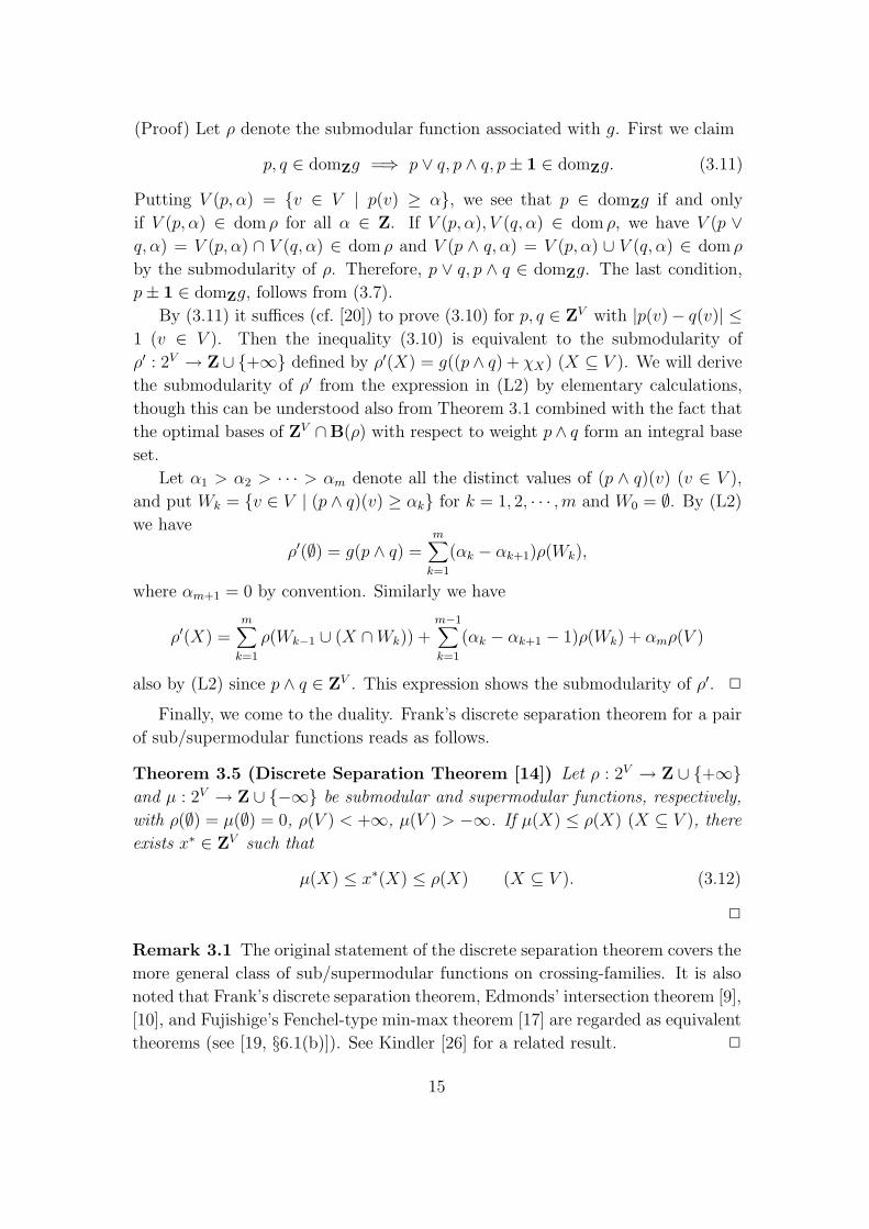
(Proof) Let ρ denote the submodular function associated with g. First we claim

p, q ∈ domZg =⇒ p ∨ q, p ∧ q, p ± 1 ∈ domZg. (3.11)

Putting V (p, α) = {v ∈ V | p(v) ≥ α}, we see that p ∈ domZg if and only

if V (p, α) ∈ dom ρ for all α ∈ Z. If V (p, α), V (q, α) ∈ dom ρ, we have V (p ∨q, α) = V (p, α) ∩ V (q, α) ∈ dom ρ and V (p ∧ q, α) = V (p, α) ∪ V (q, α) ∈ dom ρ

by the submodularity of ρ. Therefore, p ∨ q, p ∧ q ∈ domZg. The last condition,

p ± 1 ∈ domZg, follows from (3.7).

By (3.11) it suffices (cf. [20]) to prove (3.10) for p, q ∈ ZV with |p(v)− q(v)| ≤1 (v ∈ V ). Then the inequality (3.10) is equivalent to the submodularity of

ρ′ : 2V → Z ∪ {+∞} defined by ρ′(X) = g((p ∧ q) + χX) (X ⊆ V ). We will derive

the submodularity of ρ′ from the expression in (L2) by elementary calculations,

though this can be understood also from Theorem 3.1 combined with the fact that

the optimal bases of ZV ∩B(ρ) with respect to weight p∧ q form an integral base

set.

Let α1 > α2 > · · · > αm denote all the distinct values of (p ∧ q)(v) (v ∈ V ),

and put Wk = {v ∈ V | (p ∧ q)(v) ≥ αk} for k = 1, 2, · · · ,m and W0 = ∅. By (L2)

we have

ρ′(∅) = g(p ∧ q) =m∑

k=1

(αk − αk+1)ρ(Wk),

where αm+1 = 0 by convention. Similarly we have

ρ′(X) =m∑

k=1

ρ(Wk−1 ∪ (X ∩ Wk)) +m−1∑k=1

(αk − αk+1 − 1)ρ(Wk) + αmρ(V )

also by (L2) since p ∧ q ∈ ZV . This expression shows the submodularity of ρ′. 2

Finally, we come to the duality. Frank’s discrete separation theorem for a pair

of sub/supermodular functions reads as follows.

Theorem 3.5 (Discrete Separation Theorem [14]) Let ρ : 2V → Z ∪ {+∞}and µ : 2V → Z ∪ {−∞} be submodular and supermodular functions, respectively,

with ρ(∅) = µ(∅) = 0, ρ(V ) < +∞, µ(V ) > −∞. If µ(X) ≤ ρ(X) (X ⊆ V ), there

exists x∗ ∈ ZV such that

µ(X) ≤ x∗(X) ≤ ρ(X) (X ⊆ V ). (3.12)

2

Remark 3.1 The original statement of the discrete separation theorem covers the

more general class of sub/supermodular functions on crossing-families. It is also

noted that Frank’s discrete separation theorem, Edmonds’ intersection theorem [9],

[10], and Fujishige’s Fenchel-type min-max theorem [17] are regarded as equivalent

theorems (see [19, §6.1(b)]). See Kindler [26] for a related result. 2

15

The following is a conjugate reformulation of the discrete separation theorem

based on the conjugacy between the exchangeability (B-EXC) of an integral base

set and the submodularity in its support function, as expounded in Theorem 3.3

(or Theorem 3.1).

Theorem 3.6 Let B1 and B2 be integral base sets (⊆ ZV ). If they are disjoint

(B1 ∩ B2 = ∅), there exists p∗ ∈ {−1, 0, 1}V such that

inf{〈p∗, x〉 | x ∈ B1} − sup{〈p∗, x〉 | x ∈ B2} ≥ 1. (3.13)

In particular, B1 ∩ B2 = ∅ is equivalent to B1 ∩ B2 = ∅.

(Proof) By Theorem 3.1 we have Bi = ZV ∩ B(ρi) for some submodular function

ρi : 2V → Z∪{+∞} with ρi(∅) = 0 and ρi(V ) < +∞ (i = 1, 2). If ρ1(V ) 6= ρ2(V ),

take p∗ = χV or −χV . Otherwise, apply Theorem 3.5 with ρ = ρ1 and µ = ρ2#

(where ρ2#(X) = ρ2(V ) − ρ2(V − X)) to obtain some X ⊆ V with ρ(X) < µ(X).

The choice of p∗ = −χX is valid since ρ(X) = sup{〈χX , x〉 | x ∈ B1} and µ(X) =

inf{〈χX , x〉 | x ∈ B2}. 2

Remark 3.2 It should be clear that the essence of the discrete separation the-

orem (Theorem 3.5) lies in the separation for functions in the class L0, whereas

Theorem 3.6 is for M0. This conjugate pair of separation theorems will be ex-

tended in Section 5 to a pair of separation theorems, one for M-convex/concave

functions (Theorem 5.3, called the M-separation theorem) and the other for L-

convex/concave functions (Theorem 5.4, called the L-separation theorem). 2

16

4 M-convex and L-convex Functions

4.1 General concepts

For f : ZV → Z ∪ {±∞} and h : RV → R ∪ {±∞} the effective domains are

defined by

domZf = {x ∈ ZV | −∞ < f(x) < +∞}, (4.1)

domRh = {x ∈ RV | −∞ < h(x) < +∞}. (4.2)

We use the notation

argminZ(f) = {x ∈ ZV | f(x) ≤ f(y) (∀y ∈ ZV )}, (4.3)

argminR(h) = {x ∈ RV | h(x) ≤ h(y) (∀y ∈ RV )}. (4.4)

For p ∈ RV we define f [p] : ZV → R ∪ {±∞} and h[p] : RV → R ∪ {±∞} by

f [p](x) = f(x) + 〈p, x〉, h[p](x) = h(x) + 〈p, x〉. (4.5)

Obviously, f [p] : ZV → Z ∪ {±∞} if p ∈ ZV . We say that h is an extension of f

if h(x) = f(x) for x ∈ ZV .

The (integer, convex) conjugate function f• : ZV → Z ∪ {±∞} is defined by

f•(p) = sup{〈p, x〉 − f(x) | x ∈ ZV } (p ∈ ZV ). (4.6)

The mapping f 7→ f• will be called the integer convex Fenchel transformation,

or simply the Fenchel transformation. Similarly, the integer concave conjugate

function of f is defined to be f◦ : ZV → Z ∪ {±∞} given by

f◦(p) = inf{〈p, x〉 − f(x) | x ∈ ZV } (p ∈ ZV ). (4.7)

The mapping f 7→ f◦ will be called the integer concave Fenchel transformation,

or simply the Fenchel transformation if no ambiguity arises.

The (integer, convex) biconjugate function f•• : ZV → Z∪{±∞} is defined to

be (f•)•, i.e.,

f••(x) = sup{〈p, x〉 − f•(p) | p ∈ ZV } (x ∈ ZV ). (4.8)

Similarly, f◦◦ = (f◦)◦. See Examples 1.1 and 1.2 for concrete instances of f• and

f••. The biconjugate function is closely related to the convex closure f : RV →R ∪ {±∞} of f , which is defined by

f(x) = supp∈RV

[〈p, x〉 − sup

y∈ZV

(〈p, y〉 − f(y))

](x ∈ RV ). (4.9)

17

Obviously we have f••(x) ≤ f(x) for x ∈ ZV .

The subdifferential of f at x ∈ domZf , denoted ∂Rf(x), is defined by

∂Rf(x) = {p ∈ RV | f(y) − f(x) ≥ 〈p, y − x〉 (∀y ∈ ZV )}, (4.10)

where a vector p ∈ ∂Rf(x) is called, as usual, a subgradient of f at x. We are

particularly interested in subgradients that are integer vectors, and define the

integer subdifferential of f at x ∈ domZf by ∂Zf(x) = ZV ∩ ∂Rf(x), i.e.,

∂Zf(x) = {p ∈ ZV | f(y) − f(x) ≥ 〈p, y − x〉 (∀y ∈ ZV )}, (4.11)

where p ∈ ∂Zf(x) is called an integer subgradient of f at x. See Examples 1.1 and

1.2 for concrete instances of ∂Zf .

Lemma 4.1 (1) For x ∈ domZf and p ∈ ZV we have

p ∈ ∂Zf(x) ⇐⇒ x ∈ argminZ(f [−p]) ⇐⇒ f(x) + f•(p) = 〈p, x〉. (4.12)

(2) For x ∈ domZf we have f••(x) = f(x) ⇐⇒ ∂Zf(x) 6= ∅.

(Proof) (1) This is obvious from the definition.

(2) First note the obvious inequality: f••(x) ≤ f(x). If ∃ p ∈ ∂Zf(x), we see

from (4.12) that f(x) + f•(p) = 〈p, x〉. From this and the definition of f••(x) we

obtain f••(x) ≥ 〈p, x〉 − f•(p) = f(x). Conversely, if f••(x) = f(x), there exists

p ∈ ZV such that 〈p, x〉 − f•(p) = f(x), which means p ∈ ∂Zf(x). 2

For fi : ZV → Z∪{+∞} (i = 1, 2), the integer infimum convolution (or simply

the convolution) f12Z f2 : ZV → Z ∪ {±∞} is defined by

(f12Z f2)(x) = inf{f1(x1) + f2(x2) | x1 + x2 = x, x1 ∈ ZV , x2 ∈ ZV }. (4.13)

It is easy to verify that, if f12Z f2 : ZV → Z∪{+∞}, the following identities hold

true:

domZ(f12Z f2) = domZf1 + domZf2, (4.14)

(f12Z f2)• = f1

• + f2•, (4.15)

where we use the notation

domZf1 + domZf2 = {x1 + x2 | x1 ∈ domZf1, x2 ∈ domZf2} (4.16)

on the right-hand side of (4.14).

With the above notations we now introduce two classes of “convex functions”,

FE and FG. The first class FE is defined by

FE = {f : ZV → Z ∪ {+∞} |domZf 6= ∅, f(x) = f(x) (x ∈ ZV )} (4.17)

18

with f denoting the convex closure (4.9) of f . Namely, FE (with E for Extendabil-

ity) denotes the class of “convex functions” discussed in Introduction. However,

this class is too general to be interesting, as we have seen in Examples 1.1 to

1.3. This motivates us to introduce the second class FG (with G for subGradient)

defined by

FG = {f : ZV → Z ∪ {+∞} |domZf = ZV ∩ domZf 6= ∅,domZf is rationally-polyhedral,

∂Rf(x) = ∂Zf(x) 6= ∅ (x ∈ domZf)}, (4.18)

where domZf and ∂Zf(x) denote the closed convex closures of domZf and ∂Zf(x),

respectively, and a closed convex set (⊆ RV ) is said to be rationally-polyhedral if

it is described by a system of finitely many inequalities with coefficients of rational

numbers. FG is a well-behaved proper subclass of FE, as is claimed below, and

the function f of Example 1.1 is an instance that belongs to FE \ FG.

Lemma 4.2 For f ∈ FG we have the following.

(1) domZf• =∪{∂Zf(x) | x ∈ domZf} 6= ∅.

(2) domZf•• = domZf .

(3) f••(x) = f(x) (x ∈ ZV ).

(4) p ∈ ∂Zf(x) ⇐⇒ x ∈ ∂Zf•(p), where x ∈ domZf , p ∈ domZf•.

(5) ∂Zf•(p) 6= ∅ (p ∈ domZf•).

(6) f : RV → R ∪ {+∞}.(7) domRf = domZf .

(8) f(x) = f(x) (x ∈ ZV ).

(Proof) First of all, there exists x0 ∈ domZf and we have f•(p) ≥ 〈p, x0〉−f(x0) >

−∞, which shows f• : ZV → Z ∪ {+∞}. Note also

f••(x) ≤ f(x) ≤ f(x) (x ∈ ZV ). (4.19)

(1) For x ∈ domZf and p ∈ ∂Zf(x) we have f•(p) = 〈p, x〉 − f(x) < +∞ from

(4.12). Conversely, if f•(p) < +∞, there exists x ∈ domZf such that f•(p) =

〈p, x〉 − f(x), which implies again by (4.12) that p ∈ ∂Zf(x).

(2) Note first that (1) implies f•• : ZV → Z ∪ {+∞}, since supy∈ZV (〈p, y〉 −f(y)) < +∞ for p ∈ domZf•. It follows from (4.19) that domZf•• ⊇ domZf .

To show the reverse inclusion, take x ∈ ZV \ domZf . Then x 6∈ domZf by the

19

assumption that domZf = ZV ∩ domZf . Since domZf is rationally-polyhedral by

the assumption, there exists p∗ ∈ ZV such that

〈p∗, x〉 − supy∈domZf

〈p∗, y〉 ≥ 1. (4.20)

On the other hand, by (1), there exists p0 ∈ ZV such that

f•(p0) = supy∈ZV

[〈p0, x〉 − f(x)] < +∞.

Hence we obtain

f••(x) ≥ [〈p0, x〉 − f•(p0)] + [〈p − p0, x〉 − supy∈domZf

〈p − p0, y〉]

for any p ∈ ZV . The right-hand side with p = p0 + αp∗ with α ∈ Z+ is at

least as large as [〈p0, x〉 − f•(p0)] + α, which is not bounded for α ∈ Z+. Hence

x 6∈ domZf••.

(3) By Lemma 4.1 and the definition of FG.

(4) This is immediate from (4.12) combined with (3).

(5) For p ∈ domZf• we can find, by (1), x ∈ domZf such that p ∈ ∂Zf(x),

which is equivalent to x ∈ ∂Zf•(p) by (4.12). Hence ∂Zf•(p) 6= ∅.(6) In (4.9) we have supy∈ZV (〈p, y〉 − f(y)) < +∞ for p ∈ ∂Zf(x) with x ∈

domZf , just as in the proof of (1).

(7) (4.19) implies domRf ⊇ domZf , from which follows domRf ⊇ domZf

since domRf is a closed convex set. The reverse inclusion can be shown as in the

proof of (2).

(8) This follows from (3) and (4.19). 2

Remark 4.1 A comment is in order on the assumption imposed on domZf in the

definition of FG. First, if domZf is bounded (i.e., finite), this condition is always

fulfilled. Next, this technical condition cannot be omitted in general. We provide

here an example of f satisfying the other two conditions but with domZf•• 6=domZf . Let V = {1, 2}, B = {(x1, x2) ∈ Z2 | x2 ≥

√2x1 − 1/2}, and f : Z2 →

Z ∪ {+∞} be defined by

f(x1, x2) =

{0 ((x1, x2) ∈ B)

+∞ (otherwise)

Then ∂Rf(x) = ∂Zf(x) = {(0, 0)} 6= ∅ for all x ∈ B, but f••(x) = 0 for all x ∈ Z2,

which shows domZf•• = Z2 6= domZf . To verify this, note that f•(0, 0) = 0 and

f•(p) = +∞ for p ∈ Z2 \ {(0, 0)}. 2

Remark 4.2 Certainly FG identifies a class of well-behaved “convex functions,”

in which f•• = f , ∂Zf(x) 6= ∅, and ∂Zf•(p) 6= ∅ hold true, but it does not allow us

to derive the discrete separation theorem. In fact, Example 1.3 shows the failure

of discrete separation for functions f and g with f,−g ∈ FG. 2

20

4.2 M-convex functions

We say that f is M-convex if f : ZV → Z ∪ {+∞}, domZf 6= ∅ and the following

variant of the simultaneous exchange axiom holds true:

(M-EXC) For x, y ∈ domZf and u ∈ supp+(x− y) there exists v ∈ supp−(x− y)

such that

f(x) + f(y) ≥ f(x − χu + χv) + f(y + χu − χv). (4.21)

We use the notation

M = {f : ZV → Z ∪ {+∞} | f is M-convex}. (4.22)

We say that g is M-concave if −g is M-convex. The name of M-convexity/concavity,

which is intended to mean convexity/concavity related to Matroid (or matroidal

exchangeability, to be more precise), will be justified by the Extension Theorem

(Theorem 4.11) below. Recall Examples 2.1 to 2.4 for instances of M-convex

functions.

Obviously, the indicator function δB : ZV → {0, +∞} of a set B ⊆ ZV is

M-convex if and only if B is an integral base set. Thus the concept of M-convex

function is a quantitative generalization of that of integral base set, and accordingly

an integral base set could be referred to as an “M-convex set.”

We will show fundamental properties of M-convex functions with the analogy

to ordinary convex functions in mind. It is remarked that the effective domain is

unbounded in general2.

First we note the following implication of (M-EXC) for the effective domain.

Theorem 4.3 If f is M-convex, then domZf is an integral base set.

(Proof) This is immediate from (M-EXC), since in (4.21) we have x−χu +χv, y +

χu − χv ∈ domZf if x, y ∈ domZf . 2

M-convexity is invariant under the addition/subtraction of linear functions as

well as the translation and the negation of the argument, as follows. Recall the

notation (4.5).

Theorem 4.4 Let f be an M-convex function.

(1) f [−p](x) is M-convex in x for p ∈ ZV .

(2) f(a − x) and f(a + x) are M-convex in x for a ∈ ZV .

2Some of the materials presented in this subsection are immediate consequences and slightmodifications of the results of [36], [37], [38], [39], in which M-concave functions are treated underthe notation ω. In [38], [39] the effective domain is assumed to be bounded.

21

(Proof) The proofs are immediate from (M-EXC). 2

For (a, b) ∈ ZV × ZV with a ≤ b we define the interval [a, b] by

[a, b] = {x ∈ RV | a(v) ≤ x(v) ≤ b(v) (v ∈ V )}.

We denote the restriction of f to [a, b] by f ba, namely,

f ba(x) =

{f(x) (x ∈ [a, b])

+∞ (otherwise)(4.23)

M-convexity is preserved under the restriction operation.

Theorem 4.5 If f is M-convex, then f ba is M-convex for (a, b) ∈ ZV × ZV such

that domZf ∩ [a, b] 6= ∅. 2

The global optimality is guaranteed by the local optimality expressed in terms

of the discrete analogue of the directional derivative defined by

f(x, u, v) = f(x − χu + χv) − f(x) (x ∈ domZf ; u, v ∈ V ). (4.24)

The following theorem is a straightforward extension of a similar result of [7], [8]

for a matroid valuation.

Theorem 4.6 ([37]) Let f be M-convex and x ∈ domZf . Then f(x) ≤ f(y)

(∀ y ∈ ZV ) if and only if

f(x, u, v) ≥ 0 (∀u, v ∈ V ). (4.25)

(Proof) The necessity is obvious. We prove the sufficiency by induction on ||x−y||.The assumption implies f(x) ≤ f(y) for y ∈ B with ||x − y|| = 2. Suppose

||x−y|| ≥ 4. By (M-EXC) there exists x′, y′ ∈ B such that ||x−x′|| = ||y−y′|| = 2,

||x−y′|| = ||x−y||−2, and f(x)+f(y) ≥ f(x′)+f(y′). Here we have f(x′) ≥ f(x)

by the assumption and f(y′) ≥ f(x) by the induction hypothesis. Hence we obtain

f(y) ≥ f(x). 2

Integer subgradients exist for an M-convex function, namely M ⊆ FG using

the notations (4.18) and (4.22). This fact is nontrivial in view of Example 1.1.

Theorem 4.7 For an M-convex function f and x ∈ domZf ,

∂Zf(x) = {p ∈ ZV | f(x, u, v) ≥ p(v) − p(u) (u, v ∈ V )} 6= ∅. (4.26)

Moreover, ∂Rf(x) = ∂Zf(x), and hence M ⊆ FG.

22

(Proof) Similarly to (4.12), p ∈ ∂Rf(x) if and only if x ∈ argminR(f [−p]). Then

Theorem 4.6 applied to f [−p] implies

∂Rf(x) = {p ∈ RV | f(x, u, v) ≥ p(v) − p(u) (u, v ∈ V )}.

(To be precise, f [−p] is not integer-valued, but the extension of Theorem 4.6 to

this case is obvious from its proof.)

Consider a directed graph G = (V,A) with vertex set V and arc set A =

{(u, v) | x−χu + χv ∈ domZf}. We assume that γ(a) = f(x, u, v) ∈ Z is attached

to a = (u, v) ∈ A as the arc length. Then we can express ∂Rf(x) as

∂Rf(x) = {p ∈ RV | γ(a) + p(∂+a) − p(∂−a) ≥ 0 (a ∈ A)}, (4.27)

where ∂+a and ∂−a denote the initial vertex and the terminal vertex of a ∈ A,

respectively. This expression shows that a subgradient is nothing but a valid “po-

tential function” on the vertex set. According to standard results in the network

theory (cf., e.g., [30]), we see that (i) ∂Rf(x) = ∂Zf(x) and (ii) ∂Rf(x) 6= ∅ if there

is no negative cycle with respect to γ. To prove the nonexistence of a negative

cycle we observe that, for v1, v2, v3 ∈ V such that v1 6= v2 6= v3 (with the possibility

of v1 = v3), the exchange axiom (M-EXC) implies the triangle inequality

γ(v1, v2) + γ(v2, v3) ≥ γ(v1, v3) (> −∞), (4.28)

since (M-EXC) applied to x′ = x−χv2 + χv3 and y′ = x−χv1 + χv2 with u = v1 ∈supp+(x′−y′) yields v = v2 ∈ supp−(x′−y′). The triangle inequality (4.28) implies

in particular that (v1, v3) ∈ A. Note that γ(v1, v3) = 0 if v1 = v3. Furthermore we

see that any simple cycle, say consisting of v1, v2, · · · , vk, has a nonnegative length

by a repeated application of this relation to

γ(v1, v2) + γ(v2, v3) + · · · + γ(vk−1, vk) + γ(vk, v1).

Finally, the effective domain of f is an integral base set by Theorem 4.3, and

therefore domZf = ZV ∩ domZf 6= ∅ and domZf is rationally-polyhedral. This

establishes f ∈ FG. 2

The existence of integer subgradients (or the inclusion M ⊆ FG to be more

precise) allows us to apply the general lemma (Lemma 4.2) to M-convex functions.

In particular we obtain the following statements.

Theorem 4.8 For an M-convex function f we have the following.

(1) f• : ZV → Z ∪ {+∞}.(2) domZf• =

∪{∂Zf(x) | x ∈ domZf} 6= ∅.

(3) f•• = f . 2

23

The following theorem connects the concepts of M-convex functions (“con-

vex functions”) and integral base sets (“convex sets”). It is understood that

argminZ(f [−p]) is defined by (4.3) with f replaced by f [−p] though f [−p] is not

integer-valued.

Theorem 4.9 ([38, Theorem 4.4]) Let f : ZV → Z ∪ {+∞} be such that

domZf is a bounded integral base set. Then f is M-convex if and only if argminZ(f [−p])

is an integral base set for each p ∈ RV .

This theorem can be modified as follows to cover the general case of unbounded

effective domain.

Theorem 4.10 Let f : ZV → Z ∪ {+∞} be such that domZf is an integral base

set.

(1) If f is M-convex, then argminZ(f [−p]) is either an integral base set or an

empty set for each p ∈ RV .

(2) Let f ba denote the restriction of f to [a, b], as defined in (4.23). Then f is

M-convex if and only if argminZ(f ba[−p]) is an integral base set for each p ∈ RV

and (a, b) ∈ ZV × ZV such that domZf ∩ [a, b] 6= ∅.

(Proof) (1) This follows easily from (M-EXC), since in (4.21) we have x − χu +

χv, y + χu − χv ∈ argminZ(f [−p]) if x, y ∈ argminZ(f [−p]).

(2) It is easy to see from the definition that f is M-convex if and only if f ba is

M-convex for each (a, b) ∈ ZV × ZV such that domZf ba 6= ∅. Then the assertion

follows from Theorem 4.9. 2

Remark 4.3 The introduction of restrictions in the statement of Theorem 4.10(2)

is cumbersome, but seems inevitable. As an example, let V = {1, 2} and f : Z2 →Z ∪ {+∞} be defined by

f(x1, x2) =

0 ((x1, x2) = (0, 0))

1 ((x1, x2) 6= (0, 0), x1 + x2 = 0)

+∞ (otherwise)

Then domZf = {(x1, x2) ∈ Z2 | x1 + x2 = 0} is an integral base set, and

argminZ(f [−p]) is {(0, 0)} (an integral base set) if p1 = p2, and empty otherwise.

But f is not M-convex. On the other hand, we do not have such a pathological

phenomenon for f ∈ FE; see Theorem 4.11 below. 2

The following theorem justifies the name of M-convexity with reference to our

discussion about “convex functions” in Introduction. Note here that M ⊆ FG,

established in Theorem 4.7, already implies by Lemma 4.2 that M-convex functions

can be extended to convex functions. It is mentioned that this theorem has been

proven in [38] under the assumption of the boundedness of domZf .

24

Theorem 4.11 (Extension Theorem) f : ZV → Z∪{+∞} is M-convex if and

only if f : RV → R ∪ {+∞} defined by (4.9) satisfies (a), (b) and (c) below:

(a) f(x) = f(x) (x ∈ ZV ),

(b) domRf is an integral base polyhedron,

(c) For each p ∈ RV ,

argminR(f [−p]) = {x ∈ RV | f(x) − 〈p, x〉 ≤ f(x′) − 〈p, x′〉 (∀x′ ∈ RV )}

is an integral base polyhedron or an empty set.

(Proof) First we prove the “only if” part. We have f ∈ FG by Theorem 4.7.

(a) is nothing but Lemma 4.2(8). For (b) we apply Lemma 4.2(7) to obtain

domRf = domZf , which is an integral base polyhedron by Theorem 4.3. For (c)

we note argminRf [−p] = argminZf [−p], the right-hand side of which is an integral

base polyhedron by Theorem 4.10.

Next we prove the “if” part on the basis of Theorem 4.10. It is not difficult

to prove domRf = domZf in a similar manner as in Lemma 4.2. Then condition

(b) means domZf is an integral base polyhedron, whereas (a) shows domZf =

ZV ∩ domRf = ZV ∩ domZf . Therefore domZf is an integral base set. Let

(a, b) ∈ ZV × ZV be such that domZf ba 6= ∅. It is easy to see that the restriction

of f to [a, b] defined by

fb

a(x) =

{f(x) (x ∈ [a, b])

+∞ (otherwise)

has the property that argminR(fb

a[−p]) is an integral base polyhedron for each p ∈RV . Since argminR(f

b

a[−p]) contains an integral point and fb

a[−p](x) = f ba[−p](x)

for x ∈ ZV , we have

min{f b

a[−p](x) | x ∈ RV } = min{f ba[−p](x) | x ∈ ZV }

and

ZV ∩ argminR(fb

a[−p]) = argminZ(f ba[−p]).

This means that argminZ(f ba[−p]) is an integral base set. It then follows from

Theorem 4.10(2) that f is M-convex. 2

Remark 4.4 The condition (b) in Theorem 4.11 is implied by the condition (c),

since domRf is convex, domRf =∪

p argminR(f [−p]), and the following lemma

holds true. 2

Lemma 4.12 Let D =∪

i Di ⊆ RV be a convex set with Di’s being integral base

polyhedra. Then D is an integral base polyhedron.

25

(Proof) For x, y ∈ D the line segment connecting x and y is contained in D.

By considering the restrictions of D and Di’s to the interval [x ∧ y, x ∨ y] we

may assume that there are only finitely many distinct Di’s. Therefore, there

exists i such that x ∈ Di and z ≡ x + t(y − x) ∈ Di for some t > 0. For

u ∈ supp+(x− y) = supp+(x− z), the exchange property of a base polyhedron Di

guarantees the existence of v ∈ supp−(x− z) = supp−(x− y) and α > 0 such that

x − α(χu − χv) ∈ Di ⊆ D. Hence D is a base polyhedron. The integrality of D is

easy to see. 2

Next we are interested in a dual view on the subgradient inequality. By the

definition (4.10) and Theorem 4.7 (or (4.27) to be more specific) we have, for

x ∈ domZf and y ∈ ZV ,

f(y) − f(x)

≥ max{〈p, y − x〉 | p ∈ ∂Rf(x)}= max{〈p, y − x〉 | f(x, u, v) ≥ p(v) − p(u) ((u, v) ∈ A)}, (4.29)

where

A = {(u, v) | x − χu + χv ∈ domZf}.

The last expression of (4.29) can be recognized as a linear programming problem in

variable p ∈ RV . Here we introduce another linear programming problem, which

is closely related to (but not exactly the same as) the dual of this program (see

[3], [47] for the basic facts on linear programming). The variable of the new linear

program is ϕ(u, v) indexed by (u, v) ∈ A, where

A = {(u, v) | u ∈ V +, v ∈ V −, x − χu + χv ∈ domZf}

with V + = supp+(x − y) and V − = supp−(x − y) and the objective function is

defined in terms of f(x, u, v). The linear program reads

Minimize∑

(u,v)∈A

f(x, u, v)ϕ(u, v) (4.30)

subject to ϕ(u, v) ≥ 0 ((u, v) ∈ A), (4.31)∑v:(u,v)∈A

ϕ(u, v) = x(u) − y(u) (u ∈ V +), (4.32)

∑u:(u,v)∈A

ϕ(u, v) = y(v) − x(v) (v ∈ V −). (4.33)

The optimal value of the objective function of this linear program is denoted by

f(x, y), which is equal to +∞, by convention, if the linear program is infeasible.

It may be worth mentioning that this linear program represents a transportation

problem (see, e.g., [3], [30], [41], [42]) defined on a bipartite graph G(x, y) =

26

(V +, V −; A) (where (V +, V −) is the vertex bipartition and A the arc set) with arc

cost f(x, u, v). Note that the minimum of the objective function can be attained

by an integral ϕ.

Theorem 4.13 For an M-convex function f , x ∈ domZf and y ∈ ZV we have

f(x, y) = max{〈p, y − x〉 | p ∈ ∂Rf(x)} (4.34)

and hence

f(y) − f(x) ≥ f(x, y). (4.35)

(Proof) The dual of the linear program in the last expression of (4.29) is given by

Minimize∑

(u,v)∈A

f(x, u, v)ϕ(u, v) (4.36)

subject to ϕ(u, v) ≥ 0 ((u, v) ∈ A), (4.37)

∂ϕ(v) = x(v) − y(v) (v ∈ V ), (4.38)

where

∂ϕ(v) =∑

w:(v,w)∈A

ϕ(v, w) −∑

u:(u,v)∈A

ϕ(u, v) (v ∈ V ).

This represents a transshipment problem (see, e.g., [3], [30], [41], [42]) in the

network (G = (V,A), γ) used in the proof of Theorem 4.7, where γ(a) = f(x, u, v)

is now interpreted as the cost of arc a = (u, v) ∈ A, x(v) − y(v) is the supply at

vertex v ∈ V and ϕ : A → R stands for a flow. Let f(x, y) denote the optimal

value of the linear program above. Since γ satisfies the triangle inequality (4.28),

we may assume that ϕ(u, v) > 0 only if u ∈ supp+(x − y) and v ∈ supp−(x − y).

This means that f(x, y) agrees with f(x, y). On the other hand, f(x, y) is equal

to max{〈p, y−x〉 | p ∈ ∂Rf(x)} by the linear programming duality. Hence follows

(4.34), which in turn implies (4.35) when combined with the obvious inequality

(4.29). 2

Remark 4.5 Theorem 4.13 is a quantitative extension of the well-known fact (cf.

[19, Theorem 3.28]) for a submodular system that for x, y ∈ B(ρ) there exists

ϕ ∈ RA that satisfy (4.31) –(4.33) (see (3.2) for the notation B(ρ)). This fact is

expressed in our notation that f(x, y) 6= +∞ in (4.35), i.e., that the linear program

(4.30) – (4.33) has a feasible solution. It is also mentioned that Theorem 4.13 is

an extension of the “upper-bound lemma” [34, Lemma 3.4] for a valuated matroid.

2

Remark 4.6 It is natural to ask when the inequality f(y) − f(x) ≥ f(x, y) of

(4.35) is satisfied with equality. A sufficient condition, named the unique-min

27

condition, will be given later in Lemma A.2. This amounts to an extension of the

well-known “no-shortcut lemma” for matroids (cf. Kung [29] for this name; also

see Bixby-Cunningham [1, Lemma 3.7], Frank [13, Lemma 2], Iri–Tomizawa [25,

Lemma 2], Krogdahl [28], Lawler [30, Lemma 3.1 of Chap. 8], Tomizawa–Iri [51,

Lemma 3])

2

Remark 4.7 In Theorem 4.13 we have proved the inequality (4.35) by establish-

ing the identity (4.34) by means of the linear programming duality. Here is an

alternative (direct) proof of (4.35) on the basis of the exchange property (M-EXC),

which remains valid in a more general setting (cf. [37]) but is not suitable to relate

f(x, y) to subgradients. For any u1 ∈ supp+(x− y) there exists v1 ∈ supp−(x− y)

with

f(x) + f(y) ≥ f(x − χu1 + χv1) + f(y + χu1 − χv1),

which can be rewritten as

f(y) ≥ f(x, u1, v1) + f(y2)

with y2 = y + χu1 − χv1 . By the same argument applied to (x, y2) we obtain

f(y2) ≥ f(x, u2, v2) + f(y3)

for some u2 ∈ supp+(x− y2) and v2 ∈ supp−(x− y2), where y3 = y2 + χu2 − χv2 =

y + χu1 + χu2 − χv1 − χv2 . Hence

f(y) ≥ f(y3) +2∑

i=1

f(x, ui, vi).

Repeating this process we arrive at

f(y) ≥ f(x) +m∑

i=1

f(x, ui, vi) ≥ f(x) + f(x, y),

where m = ||x − y||/2, y = x − ∑mi=1 (χui

− χvi). 2

An M-convex function can be transformed to another M-convex function through

a network, just as a (poly)matroid is induced by a network [19]. Let G =

(V,A; V +, V −) be a directed graph with a vertex set V , an arc set A, a set V + of

entrances and a set V − of exits such that V +, V − ⊆ V and V + ∩ V − = ∅. Also

let c : A → Z ∪ {+∞} be an upper capacity function, c : A → Z ∪ {−∞} a lower

capacity function, and γ : A → Z a cost function. Suppose further that we are

given a function f : ZV + → Z ∪ {+∞} and put B = domZf ⊆ ZV +. A flow is a

function ϕ : A → Z and its boundary ∂ϕ : V → Z is defined by (2.1). We denote

28

by (∂ϕ)+ (resp. (∂ϕ)−) the restriction of ∂ϕ to V + (resp. V −). A flow ϕ is called

feasible if

c(a) ≤ ϕ(a) ≤ c(a) (a ∈ A), (4.39)

∂ϕ(v) = 0 (v ∈ V − (V + ∪ V −)), (4.40)

(∂ϕ)+ ∈ B. (4.41)

Define B ⊆ ZV −and f : ZV − → Z ∪ {±∞} by

B = {(∂ϕ)− | ϕ : feasible flow}, (4.42)

f(x) = inf{〈γ, ϕ〉A + f((∂ϕ)+) |ϕ : feasible flow with (∂ϕ)− = x} (x ∈ ZV −

), (4.43)

where 〈γ, ϕ〉A =∑

a∈A γ(a)ϕ(a) and f(x) = +∞ if there is no feasible ϕ with

(∂ϕ)− = x. We assume that f : ZV − → Z ∪ {+∞} and domZf 6= ∅ (namely, that

a feasible flow exists and the minimum is finite for each x ∈ B).

Then we have the following statement, an extension of the well-known fact

that, if B is an integral base set, B is also an integral base set.

Theorem 4.14 If f is M-convex, then f is also M-convex, provided f : ZV − →Z ∪ {+∞} and domZf 6= ∅.

(Proof) This statement has been established in [38], [39] when B is bounded.

The general case with unbounded B is an immediate corollary as follows. For

x, y ∈ B, take the corresponding flows, say ϕx and ϕy, that attain the minimum

on the right-hand side of (4.43). Consider the restriction f ba of f to [a, b] with

a = (∂ϕx)+ ∧ (∂ϕy)

+ and b = (∂ϕx)+ ∨ (∂ϕy)

+. Since domZf ba is bounded, the

previous result applies. Let f ba denote the M-convex function induced from f b

a.

Then for any u ∈ supp+(x − y) there exists v ∈ supp−(x − y) such that

f(x) + f(y) = f ba(x) + f b

a(y)

≥ f ba(x − χu + χv) + f b

a(y + χu − χv)

≥ f(x − χu + χv) + f(y + χu − χv).

This shows (M-EXC) for f . 2

Remark 4.8 The class of M-convex functions is (essentially) closed under the

convolution operation (4.13). A precise statement is given later in Theorem 5.8

since the proof depends on coming theorems. 2

29

4.3 L-convex functions

We introduce the other class of “convex functions,” called L-convex functions, as a

generalization of the class L0 that consists of the Lovasz extensions of submodular

functions. The L-convex functions will turn out to be the conjugate of M-convex

functions.

As we have seen in Section 3, the class L0 consists of nonnegatively homoge-

neous functions g which satisfy (cf. Lemma 3.4 and (3.7))

domZg 6= ∅, (4.44)

g(p) + g(q) ≥ g(p ∨ q) + g(p ∧ q) (p, q ∈ ZV ), (4.45)

∃r ∈ Z, ∀p ∈ ZV : g(p + 1) = g(p) + r. (4.46)

We extend the class L0 by throwing away the homogeneity condition while retain-

ing (4.44), (4.45) and (4.46). Namely we define the class L of L-convex functions

by

L = {g : ZV → Z ∪ {+∞} | g satisfies (4.44), (4.45), (4.46) }. (4.47)

Note that (4.46) implies

g(p − χX) = g(p + χV −X) − r (p ∈ ZV , X ⊆ V ). (4.48)

Remark 4.9 L-convexity is intended to be a convexity in a certain sense. In

this respect it is worth mentioning that the submodularity (4.45) alone does not

imply anything. For example, any function g : Z2 → Z ∪ {+∞} with domZg =

{(p1, p2) ∈ Z2 | p1 = p2} is submodular, whatever values it may take on domZg.

Another example is the vector rank function of a submodular system (V, ρ), which

is given by r(x) = min{ρ(X) + x(V − X) | X ⊆ V } (x ∈ RV ) and known to

be submodular and concave (see [9], [19]). The combination of (4.45) with the

other naive-looking condition (4.46) does imply the extendability of g to a convex

function, as will be shown in Theorem 4.18(3). 2

L-convexity is invariant under the addition/subtraction of linear functions as

well as the translation and the negation of the argument, as follows. Recall the

notation (4.5).

Theorem 4.15 Let g be an L-convex function.

(1) g[−x](p) is L-convex in p for x ∈ ZV .

(2) g(a − p) and g(a + p) are L-convex in p for a ∈ ZV .

(Proof) The proofs are immediate from the definition. 2

30

As the set version of L-convexity, we define D ⊆ ZV to be an L-convex set, if

D 6= ∅, (4.49)

p, q ∈ D =⇒ p ∨ q, p ∧ q ∈ D, (4.50)

p ∈ D =⇒ p ± 1 ∈ D. (4.51)

Obviously, D ⊆ ZV is an L-convex set if and only if its indicator function δD :

ZV → {0, +∞} is an L-convex function. We introduce the following notation:

0L = {δD : ZV → {0, +∞} | D is an L-convex set }. (4.52)

The following two statements hold true, as expected. In the latter theorem it

is understood that argminZ(g[−x]) is defined by (4.3) with f replaced by g[−x]

though g[−x] is not integer-valued.

Theorem 4.16 Let g be an L-convex function. Then domZg is an L-convex set.

(Proof) The proof is immediate from (4.45) and (4.46). 2

Theorem 4.17 Let g be an L-convex function. Then argminZ(g[−x]) is either an

L-convex set or an empty set for each x ∈ RV .

(Proof) Note first that argminZ(g[−x]) is nonempty only if g[−x](p+1) = g[−x](p)

(∀p ∈ ZV ), which implies (4.51). The condition (4.50) follows from (4.45). 2

Next we show that the convex closure g of g ∈ L, as defined in (4.9), can

be expressed as a localized version of the Lovasz extension of the submodular

function ρp(X) = g(p + χX) − g(p) which represents the local behaviour of g in

the neighborhood of p.

Theorem 4.18 Let g be an L-convex function.

(1) For p ∈ domZg and q ∈ [0, 1]V we have

g(p + q) = g(p) +n∑

j=1

(qj − qj+1)(g(p + χVj) − g(p)) (4.53)

under the convention 0×∞ = 0 and the indexing convention q1 ≥ q2 ≥ · · · ≥ qn as

(L2) in Section 3 that, for each q, the elements of V are indexed as {v1, v2, · · · , vn}in such a way that q(v1) ≥ q(v2) ≥ · · · ≥ q(vn); qj = q(vj), Vj = {v1, v2, · · · , vj}for j = 1, · · · , n, and qn+1 = 0.

(2) (4.53) can be rewritten as

g(p + q) = (1 − q1)g(p) +n∑

j=1

(qj − qj+1)g(p + χVj), (4.54)

31

which is a valid expression for p ∈ ZV and q ∈ [0, 1]V (being free from ∞ − ∞even for p 6∈ domZg).

(3) g(p) = g(p) (p ∈ ZV ).

(4) g(q + α1) = g(q) + αr (q ∈ RV , α ∈ R).

(5) The expression (4.53) with p ∈ domZg remains valid for q ∈ N0, where

N0 = {q ∈ RV | maxv∈V

q(v) − minv∈V

q(v) ≤ 1}. (4.55)

(Proof) (1) & (2) First, the rewriting of (4.53) to (4.54) is easy. Denote by hp(q)

the right-hand side of (4.54), which, for each p ∈ ZV , represents a piecewise-

linear function in q ∈ [0, 1]V . Let h : RV → R ∪ {+∞} be the piecewise-linear

function well-defined as h(p + q) = hp(q) by the collection {hp | p ∈ ZV }, where

the well-definedness means the consistency between “neighboring pieces,” namely,

that hp(q) = hp−χv(q + χv) for q ∈ [0, 1]V with q(v) = 0. By Lemma 3.2 each hp is

convex in the unit hypercube [0, 1]V . In other words, h is convex in the hypercube

{q ∈ RV | p ≤ q ≤ p + 1} for each p ∈ ZV . This implies further that h is a convex

function over RV , since we have

h(q − α1) = h(q) − αr (q ∈ RV , α ∈ R) (4.56)

from (4.46) and for each q ∈ RV we can find α ∈ R such that q − α1 is contained

in the interior of some unit hypercube {q′ ∈ RV | p ≤ q′ ≤ p+1}. Therefore h is a

convex function such that h(p) = g(p) for p ∈ ZV , and obviously h is the maximum

of such functions. On the other hand, g is characterized as the maximum convex

function that satisfies g(p) ≤ g(p) for p ∈ ZV . Hence follows h = g.

(3) This is immediate from (4.54) with q = 0.

(4) This is nothing but (4.56).

(5) For q ∈ N0 we have q − α1 ∈ [0, 1]V with α = minv∈V q(v), and

g(p + q) = g(p + (q − α1)) + αr

by (4). The right-hand side can be expanded according to (4.53) as

g(p + (q − α1)) + αr

= g(p) +n−1∑j=1

((qj − α) − (qj+1 − α))(g(p + χVj) − g(p))

+(qn − α)(g(p + 1) − g(p)) + αr

= g(p) +n∑

j=1

(qj − qj+1)(g(p + χVj) − g(p)).

2

32

Corollary 4.19 g ∈ L0 if and only if g ∈ L and g is nonnegatively homogeneous

(i.e., g(λp) = λg(p) for 0 ≤ λ ∈ Z and p ∈ ZV ).

(Proof) The “only if” part has been proven in Lemma 3.4 and (3.7). To show

the “if” part, first note that the nonnegative homogeneity of g implies that of

g, i.e., g(λq) = λg(q) for 0 ≤ λ ∈ R and q ∈ RV . The expression (4.53) with

p = 0 yields g(q) =∑n

j=1(qj − qj+1)g(χVj). This expression is valid for q ∈ N0 by

Theorem 4.18(5), and hence for all q ∈ RV by the nonnegative homogeneity of g.

Since g(q) = g(q) for q ∈ ZV by Theorem 4.18(3), we obtain g(q) =∑n

j=1(qj −qj+1)g(χVj

), the condition (L2) for L0. The other condition (L1) is obvious from

the submodularity (4.45). 2

Theorem 4.20 A nonempty set D ⊆ ZV is L-convex if and only if D = ZV ∩ D

and

D = {p ∈ RV | p(v) − p(u) ≤ γ(u, v) (u, v ∈ V )} (4.57)

for some γ : V × V → Z ∪ {+∞} such that γ(v, v) = 0 (v ∈ V ) and

γ(v1, v2) + γ(v2, v3) ≥ γ(v1, v3) (v1, v2, v3 ∈ V ). (4.58)

Such γ is uniquely determined by D as

γ(u, v) = supp∈D

{p(v) − p(u)} (u, v ∈ V ). (4.59)

(Proof) [“only if”] First note that γ defined by (4.59) satisfies (4.58). Denote

by P (γ) the right-hand side of (4.57). The proof of Theorem 4.18 shows that

D = ZV ∩ D and D = P (γ) for some γ, which is given by (4.59).

[“if”] For p, q ∈ P (γ) it is easy to derive (p ∨ q)(v) − (p ∨ q)(u) ≤ γ(u, v) and

(p ∧ q)(v) − (p ∧ q)(u) ≤ γ(u, v) for u, v ∈ V , which shows p ∨ q, p ∧ q ∈ P (γ).

Finally, it is obvious that p ± 1 ∈ P (γ).

[Uniqueness] If P (γ1) = P (γ2), we have γ2(u, v) ≥ supp∈P (γ1){p(v)−p(u)}. The

right-hand side here is equal, by the linear programming duality, to the shortest

path length from u to v with respect to arc length γ1 in the graph G = (V,A)

with A = {(u, v) | γ1(u, v) < +∞}, and hence is equal to γ1(u, v) by the triangle

inequality. Therefore, γ2(u, v) ≥ γ1(u, v), and by symmetry, γ2(u, v) = γ1(u, v). 2

Integer subgradients exist for an L-convex function, namely L ⊆ FG using the

notations (4.18) and (4.47).

Theorem 4.21 For an L-convex function g and p ∈ domZg, the integer subdif-

ferential ∂Zg(p) is an integral base set. Moreover, ∂Rg(p) = ∂Zg(p), and hence

L ⊆ FG.

33

(Proof) First note ∂Rg(p) = ∂Rg(p). Since N0 of (4.55) contains the origin q = 0

in its interior, we have

x ∈ ∂Rg(p) ⇐⇒ g(p + q) − g(p) ≥ 〈q, x〉 (q ∈ N0).

Using the expression (4.53) (cf. Lemma 4.18(5)) we see further that

g(p + q) − g(p) ≥ 〈q, x〉 (q ∈ N0)

⇐⇒ g(p + χX) − g(p) ≥ x(X) (X ⊆ V ); g(p + 1) − g(p) = x(V )

⇐⇒ x ∈ B(ρp),

where ρp(X) = g(p + χX) − g(p) (X ⊆ V ) and B(ρp) denotes the integral base

polyhedron associated with ρp. Hence ∂Rg(p) = B(ρp). It then follows from

Theorem 3.1 that ∂Rg(p) = ∂Zg(p) 6= ∅. Finally, domZg is rationally-polyhedral

and domZg = ZV ∩ domZg by Theorem 4.16 and Theorem 4.20. 2

The existence of integer subgradients (or the inclusion L ⊆ FG to be more

precise) allows us to apply the general lemma (Lemma 4.2) to L-convex functions.

In particular we obtain the following statements.

Theorem 4.22 For an L-convex function g we have the following.

(1) g• : ZV → Z ∪ {+∞}.(2) domZg• =

∪{∂Zg(p) | p ∈ domZg} 6= ∅.

(3) g•• = g. 2

The class of L-convex functions is essentially closed under addition.

Theorem 4.23 For L-convex functions gi (i = 1, 2), the sum g1 + g2 is also L-

convex, provided domZg1 ∩ domZg2 6= ∅.

(Proof) It is easy to verify (4.44), (4.45) and (4.46) for g1 + g2. 2

Remark 4.10 After the submission of this paper the author became aware of

a paper of Favati–Tardella [12], in which convexity for discrete functions is also

discussed. In particular the concept of submodular integrally convex functions

introduced there is closely related to that of L-convex functions. In fact, it has

been shown very recently by Fujishige–Murota [20] that these two concepts are

equivalent in a sense. 2

4.4 Conjugacy

The following theorem states that the L-convex functions and the M-convex func-

tions are both extendable to convex functions, and that they are in one-to-one

correspondence under the integer Fenchel transformation • of (4.6). It is empha-

sized that this is an extension of the conjugacy relation between M0 and L0 stated

in Theorem 3.3.

34

Theorem 4.24 Let M and L be the classes of M-convex and L-convex functions,

respectively, and FE and FG be defined by (4.17) and (4.18).

(1) M ⊆ FG ⊆ FE, L ⊆ FG ⊆ FE.

(2) M• = L, L• = M. More specifically, for f ∈ M and g ∈ L we have

f• ∈ L, g• ∈ M, f•• = f and g•• = g.

(Proof) (1) This has been proven in Theorem 4.7 and Theorem 4.21, as well as in

Lemma 4.2.

(2) By Theorem 4.8 and Theorem 4.22 it suffices to show M• ⊆ L and L• ⊆ M,

which are established in Lemmas 4.25 and 4.26 below. 2

Lemma 4.25 M• ⊆ L.

(Proof) Let f ∈ M and p ∈ domZf•. Firstly, we have f• : ZV → Z ∪ {+∞} and

domZf• 6= ∅ by Theorem 4.8.

We claim that domZf• is an L-convex set. Since f ∈ M ⊆ FG by Theorem

4.7, we have domZf• = ZV ∩ P with P =∪{∂Rf(x) | x ∈ domZf} by Lemma

4.2(1). For each x ∈ domZf , ∂Rf(x) is expressed as (4.27), and therefore P can be

represented in the form of (4.57). It then follows from Theorem 4.20 that domZf•

is an L-convex set.

For (4.46) we note from Theorem 4.3 that there exists r ∈ Z such that 〈1, x〉 = r

for all x ∈ domZf . Therefore

f•(p + 1) = sup{〈p + 1, x〉 − f(x) | x ∈ domZf} = f•(p) + r.

For the submodularity (4.45) of f• it suffices to show the submodularity (3.1) of

ρp : 2V → Z ∪ {+∞} defined by ρp(X) = f•(p + χX) − f•(p) (X ⊆ V ), since

domZf• is an L-convex set (cf. [20]). Note that ρp(∅) = 0 and ρp(V ) = r. Put

Bp = argminZ(f [−p]), which is nonempty since p ∈ domZf•. Furthermore, Bp is

an integral base set by Theorem 4.10. We claim

sup{〈p + q, x〉 − f(x) | x ∈ ZV } = sup{〈p + q, x〉 − f(x) | x ∈ Bp} (q ∈ {0, 1}V ),

(4.60)

which is proven later. Since 〈p, x〉−f(x) = f•(p) for x ∈ Bp, we can rewrite (4.60)

as

f•(p + q) − f•(p) = sup{〈q, x〉 | x ∈ Bp},

which (with q = χX) implies ρp(X) = sup{x(X) | x ∈ Bp}. This expression reveals

the submodularity of ρp by Theorem 3.1.

It remains to prove (4.60). Obviously, LHS ≥ RHS. Assume that RHS is finite,

and let z ∈ Bp be a maximizer, i.e., such that

〈p + q, z〉 − f(z) = sup{〈p + q, x〉 − f(x) | x ∈ Bp}.

35

The local optimality condition in Theorem 4.6 shows

f [−p](z, u, v) ≥ q(v) − q(u) if z − χu + χv ∈ Bp.

On the other hand, if z − χu + χv 6∈ Bp, we have

f [−p](z − χu + χv) ≥ f [−p](z) + 1,

which implies

f [−p](z, u, v) ≥ 1 ≥ q(v) − q(u)

since q ∈ {0, 1}V . Combining these two cases we obtain

f [−p](z, u, v) ≥ q(v) − q(u) (u, v ∈ V ),

that is,

f [−p − q](z, u, v) ≥ 0 (u, v ∈ V ).

Then Theorem 4.6 (the reverse direction) shows that z minimizes f [−p − q] over

ZV . Hence follows LHS = RHS in (4.60). 2

Lemma 4.26 L• ⊆ M.

(Proof) Let g ∈ L and put f = g•. We want to apply Theorem 4.10 to derive

f ∈ M.

Firstly we claim that domZf is an integral base set. Since g ∈ L ⊆ FG by

Theorem 4.21, we have domZf = domZg• = ZV ∩ D with D =∪{∂Rg(p) | p ∈

domZg} by Lemma 4.2(1). D is a convex set represented as the union of integral

base polyhedra, since D = {x ∈ RV | sup{〈p, x〉 − g(p) | p ∈ ZV } < +∞}and ∂Rg(p) = ∂Zg(p), for each p ∈ domZg, is an integral base set by Theorem

4.21. It then follows from Lemma 4.12 that D is an integral base polyhedron.

Consequently, domZf = ZV ∩ D in an integral base set.

Secondly, for p ∈ domZg it follows from (4.12) and Theorem 4.22(3) that

argminZ(f [−p]) = argminZ(g•[−p]) = ∂Zg••(p) = ∂Zg(p),

which is an integral base set by Theorem 4.21. From this it is easy to see that

the restriction f ba of f to [a, b] with (a, b) ∈ ZV × ZV has the property that

argminZ(f ba[−p]) is an integral base set for each p ∈ RV (provided domZf b

a 6= ∅).2

36

Example 4.1 Here is an example of a conjugate pair f ∈ M and g ∈ L for

V = {1, 2, 3, 4}. Let f : Z4 → Z ∪ {+∞} be defined by

f(x) =

0 (x = (1, 1, 0, 0), (0, 0, 1, 1))

−1 (x = (1, 0, 1, 0), (1, 0, 0, 1), (0, 1, 1, 0), (0, 1, 0, 1))

+∞ (otherwise)

as in Example 2.4, and g : Z4 → Z ∪ {+∞} be defined by

g(p) = max(p1 + p2, p3 + p4, p1 + p3 + 1, p1 + p4 + 1, p2 + p3 + 1, p2 + p4 + 1).

Then g• = f ∈ M and f• = g ∈ L. 2

Remark 4.11 We can regard an affine function as being M-convex and L-convex

at the same time in the following sense. Let h : ZV → Z be an affine function

(or more precisely, the restriction of an affine function over RV ). Consider V =

{v0} ∪ V by introducing a new element v0, and define f : ZV → Z ∪ {+∞} by

f(x0, x) =

{h(x) (x0 + 〈1, x〉 = 0)

+∞ (otherwise)

and g : ZV → Z by g(x0, x) = h(x−x01), where x0 ∈ Z, x ∈ ZV and (x0, x) ∈ ZV .

Then f is M-convex, g is L-convex and f(0, x) = h(x) = g(0, x) for x ∈ ZV . 2

In either case of M- and L-convexity we have defined the convexity of a subset

of ZV through the convexity of its indicator function. Namely, we have introduced

M0 = {δB : ZV → {0, +∞} | B is an M-convex set },

0L = {δD : ZV → {0, +∞} | D is an L-convex set }.

Motivated by the fact that the conjugate of an indicator function is nonnegatively

homogeneous, we define

0M = {f ∈ M | f is nonnegatively homogeneous },L0 = {g ∈ L | g is nonnegatively homogeneous },

where L0 is consistent with our previous notation for the class of the Lovasz

extensions of submodular functions (cf. Corollary 4.19). As a consequence of

the conjugacy bewteen 0L and 0M and Theorem 4.20, a member of 0M can be

identified with a distance function γ : V × V → Z ∪ {+∞} satisfying the triangle

inequality (4.58).

The conjugacy relations are summarized in Table 1.

37

Table 1: Conjugacy between M- and L-convexity

M-convexity L-convexity

Set M0 (indicator) L0 (homog.)

integral base set Lovasz extension of

(=M-convex set) submodular function

0M (homog.) 0L (indicator)

L-convex set

Function M LM-convex function L-convex function

Part II: Duality

5 Fenchel-type Duality and Separation Theo-rems

5.1 Duality theorems

The duality theorems for M- and L-convex functions stated below are derived from

Frank’s discrete separation theorem for submodular functions (Theorem 3.5) and

the following theorem established by the present author in [37].

Theorem 5.1 ([37, Theorem 4.1]) Assume that f1, f2 : ZV → Z ∪ {+∞} are

M-convex functions and let x∗ ∈ domZf1 ∩ domZf2. Then

f1(x∗) + f2(x

∗) ≤ f1(x) + f2(x) (∀x ∈ ZV )

if and only if there exists p∗ ∈ ZV such that

f1[−p∗](x∗) ≤ f1[−p∗](x) (∀x ∈ ZV ),

f2[+p∗](x∗) ≤ f2[+p∗](x) (∀x ∈ ZV ).

(Proof) A self-contained proof is provided in Appendix. 2

Remark 5.1 When f1 and f2 are affine functions (cf. Example 2.1), the above

theorem agrees with the optimality criterion (Fujishige’s potential characteriza-

tion [16]) for the weighted intersection problem for a pair of submodular systems

(see also [19]). When domZf1, domZf2 ⊆ {0, 1}V , on the other hand, which corre-

sponds to a pair of matroids, the above theorem reduces to the optimality criterion

38

[34, Theorem 4.2] for the valuated matroid intersection problem. If, in addition,

f1 is affine and f2 = 0, this criterion recovers Frank’s weight splitting theorem

[13] for the weighted matroid intersection problem, which is in turn equivalent to

Iri–Tomizawa’s potential characterization of the optimality for the independent

assignment problem [25]. 2

The following Fenchel-type min-max duality is a discrete analogue of the Fenchel

min-max duality in the ordinary convex analysis [43], [49]. This theorem has been

proved in Murota [38] under the assumption that both domZf and domZg are

bounded, in which case we have domZf• ∩ domZg◦ = ZV .

Theorem 5.2 (Fenchel-type Duality) Let f : ZV → Z∪{+∞} be an M-convex

function and g : ZV → Z ∪ {−∞} be an M-concave function such that domZf ∩domZg 6= ∅ or domZf• ∩ domZg◦ 6= ∅. Then we have

inf{f(x) − g(x) | x ∈ ZV } = sup{g◦(p) − f•(p) | p ∈ ZV }. (5.1)

If this common value is finite, the infimum is attained by some x ∈ domZf∩domZg

and the supremum is attained by some p ∈ domZf• ∩ domZg◦.

(Proof) In view of the weak duality

f(x) − g(x) ≥ g◦(p) − f•(p) (x ∈ ZV , p ∈ ZV ) (5.2)

as well as the discreteness of the problem, it suffices to prove the following two

claims:

Claim 1: If domZf∩domZg 6= ∅ and inf{f(x)−g(x) | x ∈ ZV } is finite, there exist

x∗ ∈ domZf ∩ domZg and p∗ ∈ domZf• ∩ domZg◦ such that f(x∗)− g(x∗) =

g◦(p∗) − f•(p∗).

Claim 2: If domZf•∩domZg◦ 6= ∅ and sup{g◦(p)−f•(p) | p ∈ ZV } is finite, then

domZf ∩ domZg 6= ∅.

[Proof of Claim 1] Suppose x∗ ∈ domZf ∩ domZg attains the infimum on the

left-hand side of (5.1). It follows from Theorem 5.1 with f1 = f and f2 = −g that

there exists p∗ ∈ ZV such that

f(x∗) − 〈p∗, x∗〉 ≤ f(x) − 〈p∗, x〉 (x ∈ ZV ),

g(x∗) − 〈p∗, x∗〉 ≥ g(x) − 〈p∗, x〉 (x ∈ ZV ).

This means

f(x∗) + f•(p∗) = 〈p∗, x∗〉, g(x∗) + g◦(p∗) = 〈p∗, x∗〉,

39

which in turn implies f(x∗) − g(x∗) = g◦(p∗) − f•(p∗).

[Proof of Claim 2] We will show that domZf• ∩ domZg◦ 6= ∅ and domZf ∩domZg = ∅ imply sup{g◦(p) − f•(p) | p ∈ ZV } = +∞. Take p0 ∈ domZf• ∩domZg◦. From the inequalities

f•(p) = supx∈domZf

(〈p − p0, x〉 + [〈p0, x〉 − f(x)]) ≤ supx∈domZf

〈p − p0, x〉 + f•(p0),

g◦(p) = infx∈domZg

(〈p − p0, x〉 + [〈p0, x〉 − g(x)]) ≥ infx∈domZg

〈p − p0, x〉 + g◦(p0),

we obtain

g◦(p)− f•(p) ≥

infx∈domZg

〈p − p0, x〉 − supx∈domZf

〈p − p0, x〉

+ g◦(p0)− f•(p0). (5.3)

On the other hand, since domZf ∩ domZg = ∅, Theorem 3.6 (separation theorem

for integral base sets) guarantees the existence of p∗ ∈ ZV such that

inf{〈p∗, x〉 | x ∈ domZg} − sup{〈p∗, x〉 | x ∈ domZf} ≥ 1.

This means that, for p = p0 + αp∗ with α ∈ Z+, the right-hand side of (5.3) is at

least as large as α + g◦(p0) − f•(p0), which is not bounded for α ∈ Z+. 2

Remark 5.2 In Theorem 5.2 we cannot get rid of the assumption on the effective

domains. In fact, here is an example of M-convex f and M-concave g such that

domZf ∩ domZg = ∅ and domZf• ∩ domZg◦ = ∅, for which we have

inf{f(x) − g(x) | x ∈ ZV } = +∞, sup{g◦(p) − f•(p) | p ∈ ZV } = −∞.

Let f : Z2 → Z ∪ {+∞} and g : Z2 → Z ∪ {−∞} be defined by

f(x1, x2) =

{x1 (x1 + x2 = 1)

+∞ (otherwise)g(x1, x2) =

{−x1 (x1 + x2 = −1)

−∞ (otherwise)

Then

f•(p1, p2) =

{p2 (p1 − p2 = 1)

+∞ (otherwise)g◦(p1, p2) =

{−p2 (p1 − p2 = −1)

−∞ (otherwise)

2

From the Fenchel-type duality above we can derive discrete separation theorems

for a pair of M-convex/concave functions as well as for a pair of L-convex/concave

functions.

40

Theorem 5.3 (M-Separation Theorem) Let f : ZV → Z ∪ {+∞} be an M-

convex function and g : ZV → Z ∪ {−∞} be an M-concave function such that

domZf ∩ domZg 6= ∅ or domZf• ∩ domZg◦ 6= ∅. If f(x) ≥ g(x) (x ∈ ZV ), there

exist α∗ ∈ Z and p∗ ∈ ZV such that

f(x) ≥ α∗ + 〈p∗, x〉 ≥ g(x) (x ∈ ZV ). (5.4)

(Proof) First note that (5.4) is equivalent to

f•(p∗) ≤ −α∗ ≤ g◦(p∗). (5.5)

In case domZf ∩ domZg 6= ∅, we have 0 ≤ inf{f(x) − g(x) | x ∈ ZV } < +∞ and

by Theorem 5.2 there exist x∗ ∈ domZf ∩domZg and p∗ ∈ domZf•∩domZg◦ such

that

f(x∗) − g(x∗) = g◦(p∗) − f•(p∗).

Since the left-hand side is nonnegative by the assumption, there exists α∗ ∈ Z that

satisfies (5.5).

Next we consider the case where domZf ∩domZg = ∅ and domZf•∩domZg◦ 6=∅. Theorem 5.2 shows sup{g◦(p)− f•(p) | p ∈ ZV } = +∞, which implies f•(p∗) ≤g◦(p∗) for some p∗ ∈ ZV . By choosing α∗ ∈ Z with (5.5) we obtain (5.4). (An

alternative proof can be found in [21].) 2

Theorem 5.4 (L-Separation Theorem) Let f : ZV → Z ∪ {+∞} be an L-

convex function and g : ZV → Z ∪ {−∞} be an L-concave function such that

domZf ∩ domZg 6= ∅ or domZf• ∩ domZg◦ 6= ∅. If f(p) ≥ g(p) (p ∈ ZV ), there

exist β∗ ∈ Z and x∗ ∈ ZV such that

f(p) ≥ β∗ + 〈p, x∗〉 ≥ g(p) (p ∈ ZV ). (5.6)

(Proof) A proof similar to that of Theorem 5.3 works by virtue of the conjugacy

between M-convexity and L-convexity in Theorem 4.24. (An alternative proof can

be found in [21].) 2

It should be clear that M- and L-separation theorems are conjugate to each

other, while the Fenchel-type min-max identity is self-conjugate.

Remark 5.3 Let B and B′ be integral base sets and δB and δB′ be their indicator

functions. The L-separation theorem for f = δB• and g = (−δB′)◦ reduces to the

discrete separation theorem (Theorem 3.5) for sub/supermodular functions. 2

A separation theorem for a pair of L-convex sets is stated below. Compare

this with Theorem 3.6, which asserts the discrete separation for M-convex sets

(=integral base sets).

41

Theorem 5.5 Let D1 and D2 be L-convex sets (⊆ ZV ). If they are disjoint (D1∩D2 = ∅), there exists x∗ ∈ {−1, 0, 1}V such that

inf{〈p, x∗〉 | p ∈ D1} − sup{〈p, x∗〉 | p ∈ D2} ≥ 1. (5.7)

In particular, D1 ∩ D2 = ∅ is equivalent to D1 ∩ D2 = ∅.

(Proof) Let γ1 and γ2 be defined by (4.59) for the polyhedral descriptions of D1

and D2, respectively. The expressions (4.57) for D1 and D2 show that D1∩D2 = ∅implies

D1 ∩ D2 = {p ∈ RV | p(v) − p(u) ≤ γ12(u, v) (u, v ∈ V )} = ∅

for γ12(u, v) = min{γ1(u, v), γ2(u, v)}. This means that the graph G = (V,A)

with A = {(u, v) | γ12(u, v) < +∞} contains a cycle of negative length with

respect to arc length γ12. Let v0, v1, v2, . . . , vk−1 be such a cycle with minimum

k ≥ 2. By the triangle inequalities of γ1 and γ2, it may be assumed that k is

even and γ1(v2i, v2i+1) ≤ γ2(v2i, v2i+1) and γ1(v2i+1, v2i+2) ≥ γ2(v2i+1, v2i+2) for

0 ≤ i ≤ k/2 − 1, where vk = v0. Let x∗ be such that x∗(v2i) = 1, x∗(v2i+1) = −1

for 0 ≤ i ≤ k/2 − 1, and x∗(v) = 0 otherwise. Then

infp∈D1

〈p, x∗〉 = −k/2−1∑i=0

γ1(v2i, v2i+1), supp∈D2

〈p, x∗〉 =k/2−1∑i=0

γ2(v2i+1, v2i+2)

by the minimality of k, and therefore

supp∈D2

〈p, x∗〉 − infp∈D1

〈p, x∗〉 =k/2−1∑i=0

γ1(v2i, v2i+1) +k/2−1∑i=0

γ2(v2i+1, v2i+2)

=k−1∑i=0

γ12(vi, vi+1) ≤ −1.

2

Remark 5.4 The Fenchel-type min-max identity, the M- and L-separation the-

orems can be regarded as equivalent statements, just as the Fenchel min-max

identity and the separation theorem are equivalent in the ordinary convex analysis

[43], [49]. In fact, the Fenchel-type min-max identity (Theorem 5.2) can be derived

from the M-separation theorem as follows. In the proof of Theorem 5.2 Claim 2

has been established on the basis of Theorem 3.6 (separation theorem for integral

base sets). For the case of Claim 1, we apply the M-separation theorem to f(x)−α

and g(x), where α = inf{f(x) − g(x) | x ∈ ZV }, to obtain

f(x) − α ≥ α∗ + 〈p∗, x〉 ≥ g(x) (x ∈ ZV )

42

for some α∗ ∈ Z and p∗ ∈ ZV . It then follows that

g◦(p∗) − f•(p∗) ≥ α = inf{f(x) − g(x) | x ∈ ZV },

which implies (5.1) by the weak duality (5.2). A similar (conjugate) argument

works to derive Theorem 5.2 from the L-separation theorem. It should be clear

that Theorem 5.5 above is used in place of Theorem 3.6. 2

Remark 5.5 The M-separation theorem (Theorem 5.3) is a slight extension of

the Primal Separation Theorem in [38], [39], in which both domZf and domZg are

assumed to be bounded. The L-separation theorem (Theorem 5.4), on the other

hand, is a reformulation and a slight extension of the Dual Separation Theorem

in [38], [39], which is stated for conjugate functions of M-convex/concave func-

tions under the assumption of the boundedness of the effective domains of the

M-convex/concave functions. 2

5.2 Consequences of the duality

We go on to deal with subgradients of the sum of two M-convex functions and

the convolution of two L-convex functions. These results will have important

consequences in the Lagrange duality framework developed later.

The following identity is nontrivial in view of Example 1.2. In fact it is a

duality assertion in disguise (and as such the proof relies on the duality theorem).

Compare this with a similar identity [43, Theorem 23.8] in the ordinary convex

analysis.

Theorem 5.6 For M-convex functions fi (i = 1, 2),

∂Z(f1 + f2)(x) = ∂Zf1(x) + ∂Zf2(x) (x ∈ domZf1 ∩ domZf2).

In particular, ∂Z(f1 + f2)(x) 6= ∅ for x ∈ domZf1 ∩ domZf2.

(Proof) For each i = 1, 2, we see pi ∈ ∂Zfi(x) ⇐⇒ x ∈ argminZ(fi[−pi]),

as noted in (4.12). Obviously, the latter conditions for i = 1, 2 imply that x ∈argminZ(f1[−p1] + f2[−p2]) = argminZ((f1 + f2)[−p1 − p2]), i.e., p1 + p2 ∈ ∂Z(f1 +

f2)(x). Therefore ∂Z(f1+f2)(x) ⊇ ∂Zf1(x)+∂Zf2(x). To show the reverse inclusion

we need a duality result. Suppose p ∈ ∂Z(f1 + f2)(x). Since it is equivalent to

x ∈ argminZ((f1 + f2)[−p]) = argminZ(f1 + f2[−p]), Theorem 5.1 applied to f1

and f2[−p] implies the existence of p1 ∈ ZV such that x ∈ argminZ(f1[−p1]) and

x ∈ argminZ(f2[−p + p1]). Putting p2 = p − p1 we obtain p = p1 + p2 with

pi ∈ ∂Zfi(x) for i = 1, 2. Therefore ∂Z(f1 + f2)(x) ⊆ ∂Zf1(x) + ∂Zf2(x). The

final claim follows from the established identity since ∂Zfi(x) 6= ∅ for i = 1, 2 by

Theorem 4.7. 2

43

Remark 5.6 The special case of the above theorem for matroid valuations has

been given in [36, Theorem 4.7]. 2

The following assertion, though looking similar to an obvious relation (4.15),

relies also on the duality in the form encoded in Theorem 5.6.

Theorem 5.7 Let fi (i = 1, 2) be M-convex functions.

(1) (f1 + f2)• = f1

•2Z f2•, provided domZf1 ∩ domZf2 6= ∅.

(2) (f1 + f2)•• = f1 + f2.

(Proof) (1) Let p ∈ domZ(f1 + f2)•. If p = p1 + p2 we have

(f1 + f2)•(p) = sup{〈p, x〉 − f1(x) − f2(x) | x ∈ ZV }

≤2∑

i=1

sup{〈pi, x〉 − fi(x) | x ∈ ZV }

= f1•(p1) + f2

•(p2),

which shows (f1+f2)•(p) ≤ (f1

•2Z f2•)(p). For the reverse direction of the inequal-

ity, take x ∈ argminZ((f1 + f2)[−p]), which means p ∈ ∂Z(f1 + f2)(x) by (4.12).

Then Theorem 5.6 guarantees the decomposition p = p1 + p2 with pi ∈ ∂Zfi(x)

(i = 1, 2), and therefore

(f1 + f2)•(p) = 〈p, x〉 − f1(x) − f2(x)

=2∑

i=1

(〈pi, x〉 − fi(x))

= f1•(p1) + f2

•(p2)

≥ (f1•2Z f2

•)(p).

(2) Both (f1 + f2)•• and f1 + f2 are identically equal to +∞ if domZf1 ∩

domZf2 = ∅. Otherwise, by (1), (4.15) and Theorem 4.8(3) we obtain (f1+f2)•• =

(f1•2Z f2

•)• = f1•• + f2

•• = f1 + f2. 2

Remark 5.7 The second statement of Theorem 5.6 (i.e., ∂Z(f1 + f2)(x) 6= ∅) is

not contained in the latter half of Theorem 4.7. Nor is Theorem 5.7(2) a special

case of Theorem 4.8(3). This is because the sum of two M-convex functions is not

necessarily M-convex. 2

The class of M-convex functions is essentially closed under the infimum convo-

lution operation (4.13).

Theorem 5.8 Let fi (i = 1, 2) be M-convex functions and f12Z f2 : ZV → Z ∪{±∞} be the convolution defined by (4.13).

44

(1) f12Z f2 is M-convex, provided f12Z f2 : ZV → Z ∪ {+∞} (i.e., if it does

not take the value −∞).

(2) If (f12Z f2)(x0) = −∞ for some x0 ∈ ZV , then

(f12Z f2)(x) =

{−∞ (x ∈ domZf1 + domZf2)

+∞ (otherwise)

This is the case if and only if domZf1• ∩ domZf2

• = ∅.

(Proof) (1) First recall the relation (4.15): (f12Z f2)• = f1

•+f2•. By the conjugacy

between M-convexity and L-convexity (Theorem 4.24) the assertion is equivalent to

the fact (Theorem 4.23) that the sum of two L-convex functions is again L-convex,

if their effective domains are not disjoint.

(2) The Fenchel-type min-max identity (Theorem 5.2) shows that

infy∈ZV

(f1(y) + f2(x − y)) = supp∈ZV

(〈p, x〉 − f1•(p) − f2

•(p)),

for each x ∈ domZf1 + domZf2. The assumption (f12Z f2)(x0) = −∞ implies

that x0 ∈ domZf1 + domZf2 and hence the right-hand side above for x = x0

is equal to −∞, which is equivalent to domZf1• ∩ domZf2

• = ∅. Hence follows

(f12Z f2)(x) = −∞ for all x ∈ domZf1 + domZf2. Finally it is obvious that

(f12Z f2)(x) = +∞ for x 6∈ domZf1 + domZf2. 2

Remark 5.8 We have f12Z f2 : ZV → Z∪{+∞} if dom f1 or dom f2 is bounded,

and [38, Theorem 6.10] gives (1) of the above theorem in the case where both

dom f1 and dom f2 are bounded. 2

We now turn to the infimum convolution g12Z g2 of two L-convex functions gi

(i = 1, 2). First we observe the following fact.

Lemma 5.9 Let gi (i = 1, 2) be L-convex functions and g12Z g2 : ZV → Z∪{±∞}be the convolution defined by (4.13). If (g12Z g2)(p0) = −∞ for some p0 ∈ ZV ,

then

(g12Z g2)(p) =

{−∞ (p ∈ domZg1 + domZg2)

+∞ (otherwise)

This is the case if and only if domZg1• ∩ domZg2

• = ∅.

(Proof) The proof is similar to that of Theorem 5.8(2). 2

The subdifferential of the infimum convolution of two L-convex functions has

a nice combinatorial characterization. Namely, it is a nonempty set that can be

expressed as the intersection of two integral base sets.

45

Theorem 5.10 Let gi (i = 1, 2) be L-convex functions such that g12Z g2 : ZV →Z ∪ {+∞}. For p ∈ domZ(g12Z g2) there exists pi ∈ domZgi (i = 1, 2) such that

p = p1 + p2 and

∂Z(g12Z g2)(p) = ∂Zg1(p1) ∩ ∂Zg2(p2) 6= ∅. (5.8)

(Proof) Put fi = gi• (i = 1, 2), g = g12Z g2 and f = f1 + f2. Then fi ∈ M

(i = 1, 2) by Theorem 4.24, and g• = f by (4.15) and f• = g by Theorem 5.7(1).

Then (4.12) shows

x ∈ ∂Zg(p) ⇐⇒ p ∈ ∂Zf(x) ⇐⇒ x ∈ argminZ(f [−p]).

Note here that argminZ(f [−p]) 6= ∅ for p ∈ domZf• = domZg. Also it follows

from Theorem 5.6 that p ∈ ∂Zf(x) if and only if p = p1 + p2 for some pi ∈ ∂Zfi(x)

(i = 1, 2), in which pi ∈ ∂Zfi(x) is equivalent to x ∈ ∂Zgi(pi). 2

Theorem 5.11 For L-convex functions gi (i = 1, 2) such that g12Z g2 : ZV →Z ∪ {+∞}, we have (g12Z g2)

•• = g12Z g2.

(Proof) By (4.15) we have (g12Z g2)• = g1

•2Z g2•. Since gi

• ∈ M (i = 1, 2), we

have by Theorem 5.7(1) and Theorem 4.22 that

(g1•2Z g2

•)• = g1••2Z g2

•• = g12Z g2.

2

The above theorems would justify to give names to the class of functions that

can be represented as the sum of two M-convex functions as well as to the class

of functions that can be represented as the convolution of two L-convex functions.

We say f : ZV → Z ∪ {+∞} is M2-convex if it can be represented as the sum

of two M-convex functions, and g : ZV → Z ∪ {+∞} is L2-convex if it can be

represented as the convolution of two L-convex functions. The classes of the M2-

and L2-convex functions are denoted respectively by

M2 = {f : ZV → Z ∪ {+∞} |domZf 6= ∅, f = f1 + f2 (∃f1, f2 ∈ M)}, (5.9)

L2 = {g : ZV → Z ∪ {+∞} |domZg 6= ∅, g = g12Z g2 (∃g1, g2 ∈ L)}. (5.10)

Then the above theorems are rephrased as follows. Recall the notations FE

and FG defined by (4.17) and (4.18).

46

Theorem 5.12

(1) M2 ⊆ FG ⊆ FE. In particular, ∂Zf(x) 6= ∅ (x ∈ domZf) and f•• = f for

f ∈ M2.

(2) L2 ⊆ FG ⊆ FE. In particular, ∂Zg(p) 6= ∅ (p ∈ domZg) and g•• = g for

g ∈ L2.

(3) M2• = L2, L2

• = M2.

(Proof) (1) This follows from Theorems 5.6, 5.7(2) and 4.7.

(2) This follows from Theorems 5.10, 5.11 and 4.21.

(3) This follows from Theorem 5.7(1) and (4.15). 2

47

6 Lagrange Duality for Optimization

6.1 Overview

On the basis of the fundamental theorems established so far, we shall develop in

this section a Lagrange duality theory for (nonlinear) integer program:

P: Minimize c(x) subject to x ∈ B, (6.1)

where c : ZV → Z∪{+∞} and ∅ 6= B ⊆ ZV . The canonical “convex” case consists

of the problems in which

(REG) B is an integral base set,

(OBJ) c is M-convex.

We follow Rockafellar’s conjugate duality approach [44] to convex/nonconvex

programs in nonlinear optimization. In fact, the whole scenario of the present

theory is a straightforward adaptation of it, whereas the technical development

leading to a strong duality assertion for “convex” programs relies heavily on the

fundamental theorems established in the previous sections. An adaptation of the

augmented Lagrangian function in nonlinear programming affords a duality frame-

work that covers “nonconvex” programs.

In the canonical “convex” case, the problem dual to P turns out to be a max-

imization of an L-concave (or L2-concave) function and the strong duality holds

between the primal/dual pair of problems. This is a consequence of the conju-

gacy between M- and L-convexity (or between M2- and L2-convexity) and the

Fenchel-type duality theorem (Theorem 5.2). Thus the classes of M2-/L2-convex

functions, introduced in Section 5.2 as extensions of M-/L-convex functions, play

an important role in this section.

In the literature of integer programming [41], [42], can be found a number

of duality frameworks such as the subadditive duality. The present approach is

distinguished from those existing ones in that:

1. It is primarily concerned with nonlinear objective functions.

2. The theory parallels the perturbation-based duality formalism in nonlinear

programming.

3. In particular, the dual problem is derived from an embedding of the given

problem in a family of perturbed problems with a certain convexity in the

direction of perturbation.

4. It identifies M-convex programs as the well-behaved core structure to be

compared to convex programs in nonlinear programming.

48

6.2 General duality framework

We describe the general framework, in which neither (REG) nor (OBJ) is assumed.

This is a straightforward adaptation of the existing Lagrange duality framework

in nonlinear programming, in particular, Rockafellar’s conjugate duality approach

[44] to convex/nonconvex programs. We follow the notation of [44] to clarify the

parallelism.

First we rewrite the problem P as

P: Minimize f(x) subject to x ∈ ZV (6.2)

with

f(x) = c(x) + δB(x), (6.3)

where δB : ZV → {0, +∞} is the indicator function of B (i.e., δB(x) = 0 if x ∈ B,

and = +∞ otherwise). Let us say that the problem P is feasible if f(x) < +∞ for

some x ∈ ZV .

Adopting the basic idea of the Lagrange duality theory in nonlinear program-

ming we embed the optimization problem P in a family of perturbed problems.

As the perturbation of f we consider F : ZV × ZU → Z ∪ {+∞}, with U being a

finite set, such that

F (x, 0) = f(x), (6.4)

F (x, ·)•• = F (x, ·) for each x ∈ ZV . (6.5)

Here the second condition (6.5) means that the integer biconjugate of F (x, u) as

a function in u for each fixed x agrees with F (x, u) itself.

Remark 6.1 Lemma 4.2(3) shows that the condition (6.5) is satisfied if, for each

x, either F (x, ·) ≡ +∞ or F (x, ·) ∈ FG, where FG is defined in (4.18). Recall in

this connection that M ⊆ M2 ⊆ FG and L ⊆ L2 ⊆ FG. 2

The resulting family of optimization problems, parametrized by u ∈ ZU , reads:

P(u): Minimize F (x, u) subject to x ∈ ZV . (6.6)

We define the optimal value function ϕ : ZU → Z ∪ {±∞} by

ϕ(u) = inf{F (x, u) | x ∈ ZV } (u ∈ ZU), (6.7)

and the Lagrangian function K : ZV × ZU → Z ∪ {±∞} by

K(x, y) = inf{F (x, u) + 〈u, y〉 | u ∈ ZU} (x ∈ ZV , y ∈ ZU). (6.8)

For each x ∈ ZV , the function K(x, ·) : y 7→ K(x, y) is the integer concave Fenchel

conjugate of the function −F (x, ·) : u 7→ −F (x, u).

Our assumptions (6.4) and (6.5) on the perturbation F (x, u) enable us to claim

the following.

49

Lemma 6.1

(1) F (x, u) = sup{K(x, y) − 〈u, y〉 | y ∈ ZU} (x ∈ ZV , u ∈ ZU).

(2) f(x) = sup{K(x, y) | y ∈ ZU} (x ∈ ZV ).

(Proof) (1) Abbreviate F (x, u) and K(x, y) to F (u) and K(y), respectively. We

have F •(y) = −K(−y) by the definition (6.8), while F (u) = F ••(u) by the as-

sumption (6.5). Therefore we obtain

F (u) = F ••(u) = supy

(〈u, y〉 + K(−y)) = supy

(K(y) − 〈u, y〉).

(2) This follows from (1) with u = 0 and (6.4). 2

We define the dual problem to P as

D: Maximize g(y) subject to y ∈ ZU , (6.9)

where the objective function g : ZU → Z ∪ {±∞} is defined by

g(y) = inf{K(x, y) | x ∈ ZV } (y ∈ ZU). (6.10)

We say that the problem D is feasible if g(y) > −∞ for some y ∈ ZU . It is

remarked that g(y) < +∞ for all y ∈ ZU if the problem P is feasible; for, g(y) ≤K(x, y) ≤ F (x, 0) = f(x) for all x ∈ ZV .

We use the following notations:

inf(P) = inf{f(x) | x ∈ ZV },sup(D) = sup{g(y) | y ∈ ZU},opt(P) = {x ∈ ZV | f(x) = inf(P)},opt(D) = {y ∈ ZU | g(y) = sup(D)}.

We write min(P) instead of inf(P) if the problem P is feasible and the infimum is

finite, where it is noted that the infimum is attained (i.e., opt(P) 6= ∅) in such a

case. Similarly, we write max(D) for sup(D) if the problem D is feasible and the

supremum is finite, in which case the supremum is attained (i.e., opt(D) 6= ∅).

Theorem 6.2 (Weak Duality) inf(P) ≥ sup(D).

(Proof) We have

g(y) = infx

K(x, y) = infx

infu

(F (x, u) + 〈u, y〉)≤ inf

x(F (x, 0) + 〈0, y〉) = inf

xf(x) = inf(P).

Hence, sup(D) = supy g(y) ≤ inf(P). 2

50

Corollary 6.3 If inf(P) = −∞ or sup(D) = +∞, then inf(P) = sup(D). 2

Our main interest lies, of course, in the strong duality, namely, the case where

the equality holds with a finite value in the weak duality above.

Theorem 6.4

(1) g(y) = −ϕ•(−y).

(2) sup(D) = ϕ••(0).

(3) inf(P) = ϕ(0).

(4) inf(P) = sup(D) ⇐⇒ ϕ(0) = ϕ••(0).

(5) If inf(P) is finite, then min(P) = max(D) ⇐⇒ ∂Zϕ(0) 6= ∅.(6) If min(P) = max(D), then opt(D) = −∂Zϕ(0).

(Proof) (1) By the definitions we have

−ϕ•(−y) = − supu

(〈u,−y〉 − ϕ(u)) = infu

(ϕ(u) + 〈u, y〉)

= infu

(infx

F (x, u) + 〈u, y〉) = infx

infu

(F (x, u) + 〈u, y〉)= inf

xK(x, y) = g(y).

(2) By using (1) we have

sup(D) = supy

g(y) = supy

(〈0,−y〉 − ϕ•(−y))

= supy

(〈0, y〉 − ϕ•(y)) = ϕ••(0).

(3) This is obvious from (6.4) and (6.7).

(4) The equivalence is due to (2) and (3).

(5)–(6) We have the following chain of equivalence: y ∈ −∂Zϕ(0) ⇐⇒ ϕ(u)−ϕ(0) ≥ 〈u,−y〉 (∀u ∈ ZU) ⇐⇒ infu(ϕ(u) + 〈u, y〉) = ϕ(0) ⇐⇒ g(y) = ϕ(0),

where infu(ϕ(u) + 〈u, y〉) = g(y) is shown in the proof of (1). This implies the

claims when combined with the weak duality (Theorem 6.2). 2

Theorem 6.5 (Saddle-Point Theorem)

min(P) = max(D) if and only if there exist x ∈ ZV , y ∈ ZU such that K(x, y) is

finite and

K(x, y) ≤ K(x, y) ≤ K(x, y) (x ∈ ZV , y ∈ ZU).

If this is the case, we have x ∈ opt(P) and y ∈ opt(D).

51

(Proof) By Lemma 6.1(2) we have f(x) = supy K(x, y), whereas g(y) = infx K(x, y)

by the definition (6.10). In view of the weak duality (Theorem 6.2) and the rela-

tion:

f(x) = supy

K(x, y) ≥ K(x, y) ≥ infx

K(x, y) = g(y),

we see that

min(P) = max(D)

⇐⇒ ∃ x,∃ y : f(x) = g(y)

⇐⇒ ∃ x,∃ y : supy

K(x, y) = K(x, y) = infx

K(x, y).

2

6.3 Augmented Lagrangian based on M-convexity

As the perturbation F , we choose F = Fr : ZV × ZV → Z ∪ {+∞} defined by

Fr(x, u) = c(x) + δB(x + u) + r(u) (x, u ∈ ZV ), (6.11)

where r : ZV → Z ∪ {+∞} is an M-convex function with r(0) = 0. (We take

V as the U in the general framework.) The special case with r = 0 is naturally

distinguished by subscript 0. Namely,

F0(x, u) = c(x) + δB(x + u) (x, u ∈ ZV ). (6.12)

We single out the case of r = 0 because the technical development in this special

case can be made within the framework of M-/L-convex functions, whereas the

general case involves M2-/L2-convex functions.

Throughout this section we assume (REG), i.e., that B is an integral base set,

which assumption is not substantially restrictive, as is discussed later in Remark

6.2.

We use subscript r to denote the quantities derived from Fr, namely,

ϕr(u) = inf{Fr(x, u) | x ∈ ZV } (u ∈ ZV ), (6.13)

Kr(x, y) = inf{Fr(x, u) + 〈u, y〉 | u ∈ ZV } (x, y ∈ ZV ), (6.14)

gr(y) = inf{Kr(x, y) | x ∈ ZV } (y ∈ ZV ), (6.15)

sup(Dr) = sup{gr(y) | y ∈ ZV }.

Our choice of the perturbation (6.11) is legitimate, meeting the requirements

(6.4) and (6.5), as follows.

52

Lemma 6.6 Assume (REG).

(1) Fr(x, 0) = f(x) (x ∈ ZV ).

(2) For each x ∈ ZV , F0(x, u) is M-convex in u or F0(x, u) = +∞ for all u.

(3) For each x ∈ ZV , Fr(x, u) is M2-convex in u or Fr(x, u) = +∞ for all u.

(4) Fr(x, u) = sup{Kr(x, y) − 〈u, y〉 | y ∈ ZV } (x, u ∈ ZV ).

Assume (REG) and (OBJ).

(5) For each u ∈ ZV , Fr(x, u) is M2-convex in x or Fr(x, u) = +∞ for all x.

(Proof) (1) This follows from r(0) = 0.

(2) We have F0(x, u) = +∞ unless x ∈ domZc. For each x, δB(x+u) = δB−x(u)

is the indicator function of B−x (translation of B by x), which is again an integral

base set. Therefore δB(x + u) is M-convex in u.

(3) We have Fr(x, u) = +∞ unless x ∈ domZc. Besides δB(x + u), r(u) is

also M-convex by the assumption. Hence Fr(x, ·) is the sum of two M-convex

functions for each x ∈ domZc. By definition, such a function is either M2-convex

or identically equal to +∞.

(4) It follows from (3) and Theorem 5.12(1) that the condition (6.5) is satisfied.

Then Lemma 6.1(1) establishes this.

(5) We have Fr(x, u) = +∞ unless u ∈ domZr. δB(x + u) = δB−u(x) is M-

convex in x and c(x) is M-convex by the assumption. Hence Fr(·, u) is the sum

of two M-convex functions for each u ∈ domZr. By definition, such a function is

either M2-convex or identically equal to +∞. 2

The Lagrangian function Kr(x, y) enjoys the following properties. It should be

clear that δB• is the integer convex Fenchel conjugate of the indicator function of

B, and that δ−B2Z r[y] means the infimum convolution of the indicator function

of −B = {x | −x ∈ B} and r[y](u) = r(u) + 〈u, y〉.

Lemma 6.7

(1) K0(x, y) =

{c(x) − 〈x, y〉 − δB

•(−y) (x ∈ domZc, y ∈ ZV )

+∞ (x 6∈ domZc, y ∈ ZV )

(2) Kr(x, y) =

{c(x) + (δ−B2Z r[y])(−x) (x ∈ domZc, y ∈ ZV )

+∞ (x 6∈ domZc, y ∈ ZV )

(Proof) (1) Assume x ∈ domZc. Substituting (6.12) into (6.14) we obtain

K0(x, y) = inf{c(x) + δB(x + u) + 〈u, y〉 | u ∈ ZV }= inf{c(x) + δB(u) + 〈u − x, y〉 | u ∈ ZV }= c(x) − 〈x, y〉 + inf{〈u, y〉 | u ∈ B}= c(x) − 〈x, y〉 − δB

•(−y).

53

(2) Assume x ∈ domZc. Substituting (6.11) into (6.14) we obtain

Kr(x, y) = inf{c(x) + δB(x + u) + r(u) + 〈u, y〉 | u ∈ ZV }= c(x) + inf{δ−B(−x − u) + r[y](u) | u ∈ ZV }= c(x) + (δ−B2Z r[y])(−x).

2

Theorem 6.8 Assume (REG).

(1) For each x ∈ ZV , K0(x, y) is L-concave in y or K0(x, y) = +∞ for all y.

(2) For each x ∈ ZV , Kr(x, y) is L2-concave in y or Kr(x, y) = +∞ for all y.

Assume (REG) and (OBJ).

(3) For each y ∈ ZV , K0(x, y) is M-convex in x or K0(x, y) ∈ {+∞,−∞} for

all x.

(4) For each y ∈ ZV , Kr(x, y) is M2-convex in x or Kr(x, y) ∈ {+∞,−∞}for all x.

(Proof) (1) For each x ∈ ZV , K0(x, ·) is the integer concave Fenchel conjugate

of the function −F0(x, ·). Since F0(x, ·) ∈ M or ≡ +∞ by Lemma 6.6(2) and

M• = L by Theorem 4.24, we see that K0(x, ·) is L-concave or ≡ +∞.

(An alternative direct proof can be obtained from the expression of Lemma

6.7(1) as follows: Since δB is M-convex by (REG), δB• is L-convex by the conjugacy.

It then follows that 〈x, y〉 + δB•(−y) is also L-convex in y.)

(2) Similarly, for each x ∈ ZV , Kr(x, ·) is the integer concave Fenchel conjugate

of the function −Fr(x, ·). Since Fr(x, ·) ∈ M2 or ≡ +∞ by Lemma 6.6(3) and

M2• = L2 by Theorem 5.12(3), we see that Kr(x, ·) is L2-concave or ≡ +∞.

(3) The M-convexity of c implies that of c(x) − 〈x, y〉 for each y in the ex-

pression of K0 in Lemma 6.7(1). Hence K0(·, y) is M-convex if δB•(−y) is finite.

(4) In the expression of Kr(x, y) in Lemma 6.7(2) we see that the second term

(δ−B2Z r[y])(−x) is M-convex or ∈ {+∞,−∞} since it is the convolution of two

M-convex functions (cf. Theorems 4.4 and 5.8). 2

In the case of M-convex programs the dual objective function gr and the optimal

value function ϕr are well-behaved, as follows.

Theorem 6.9 Assume (REG) and (OBJ).

(1) g0 is L-concave or g0(y) = −∞ for all y.

(2) gr is L2-concave, or gr(y) = −∞ for all y, or gr(y) = +∞ for all y.

(3) ϕ0 is M-convex or ϕ0(u) ∈ {+∞,−∞} for all u.

(4) ϕr is M2-convex or ϕr(u) ∈ {+∞,−∞} for all u.

54

(Proof) We prove (1), (3), (4) and finally (2).

(1) Using Lemma 6.7(1) we obtain

g0(y) = infx

K0(x, y) = infx

(c(x) − 〈x, y〉) − δB•(−y) = −c•(y) − δB

•(−y). (6.16)

This shows g0 is L-concave or ≡ −∞ , since the sum of two L-concave functions is

again L-concave, provided the effective domains of the summands are not disjoint

(cf. Theorem 4.23).

(3) We have ϕ0(u) = infx(c(x) + δB(x + u)) = (c2Z δ−B)(−u). The assertion

follows from Theorem 5.8.

(4) It follows from Fr(x, u) = F0(x, u) + r(u) that ϕr(u) = +∞ unless u ∈domZr and that ϕr(u) = ϕ0(u) + r(u) if u ∈ domZr. If ϕ0 ∈ M, then ϕr ∈ M2 or

ϕr ≡ +∞. If ϕ0(u) ∈ {+∞,−∞}, then ϕr(u) ∈ {+∞,−∞}.(2) First recall the relation gr(y) = −ϕr

•(−y) (cf. Theorem 6.4(1)). If

ϕr ∈ M2, the conjugacy between L2 and M2 (cf. Theorem 5.12) implies the

L2-concavity of gr. If ϕr ≡ +∞, then gr ≡ −∞. If ϕr(u) = −∞ for some u, then

gr ≡ +∞. 2

The strong duality holds true for M-convex programs with the Lagrangian

function Kr(x, y).

Theorem 6.10 (Strong Duality) Assume (REG), (OBJ) and that the prob-

lem P is feasible and bounded from below (i.e., inf(P) 6= ±∞).

(1) min(P) = ϕr(0) = ϕr••(0) = max(Dr).

(2) opt(Dr) = −∂Zϕr(0).

(Proof) Since ϕr(0) is finite by the assumption, ϕr is M2-convex by Theorem

6.9(4) and hence ∂Zϕr(0) 6= ∅ by Theorem 5.12(1). Then the assertions follow

from Theorem 6.4. 2

It should be emphasized that the M-convexity of the objective function c is a

sufficient condition and not an absolute prerequisite for the strong duality to hold.

Example 6.1 Let us consider the case where c(x) is a linear function on another

integral base set B′ ⊆ ZV . The primal problem with c(x) = 〈x,w〉+ δB′(x) (where

w ∈ ZV denotes the weight vector) reads:

P: Minimize 〈x,w〉 subject to x ∈ B ∩ B′. (6.17)

The Lagrangian function K0 is given by

K0(x, y) =

{〈x, w − y〉 + infz∈B〈z, y〉 (x ∈ B′, y ∈ ZV )

+∞ (x 6∈ B′, y ∈ ZV )(6.18)

55

from which is derived the dual problem:

D: Maximize(

infx∈B′

〈x,w − y〉 + infz∈B

〈z, y〉)

subject to y ∈ ZV .

(6.19)

The strong duality for this pair of problems is equivalent to Fujishige’s potential

characterization [16] (see also [19]) for the weighted intersection problem for a pair

of submodular systems, which is an extension of Frank’s weight splitting theorem

[13] for the weighted matroid intersection problem and Iri–Tomizawa’s potential

characterization of the optimality for the independent assignment problem [25].

For a concrete instance, take V = {1, 2}, B = {(x1, x2) ∈ Z2 | x1 ≥ 0, x1+x2 =

0}, B′ = {(x1, x2) ∈ Z2 | x1 ≤ 1, x1 + x2 = 0}. We have B ∩ B′ = {(0, 0), (1,−1)}and

K0(x, y) =

〈x,w − y〉 ((x1, x2) ∈ B′, y1 ≥ y2)

−∞ ((x1, x2) ∈ B′, y1 < y2)

+∞ (otherwise).

(6.20)

2

Remark 6.2 In this section we have assumed (REG) throughout. This is not

really a restriction, since any problem can be transformed into such a form. Given

a problem described by (c, B), consider V = {v0}∪V by introducing a new element

v0, choose B ⊆ ZV to be an integral base set such that B ⊇ B′, where

B′ = {(x0, x) ∈ ZV | x ∈ B, x0 + 〈1, x〉 = 0},

and define c : ZV → Z ∪ {+∞} by

c(x0, x) =

c(x) (x0 + 〈1, x〉 = 0, (x0, x) 6∈ B \ B′)

c(x) + α (x0 + 〈1, x〉 = 0, (x0, x) ∈ B \ B′)

+∞ (x0 + 〈1, x〉 6= 0)

with a big number α. Then the problem described by (c, B) meets the condition

(REG). For example, we can take B = {(x0, x) ∈ ZV | x0 + 〈1, x〉 = 0}. 2

6.4 Symmetry in duality

In the previous section we have derived the dual problem D from the primal P by

means of a perturbation function F (x, u) such that F (x, 0) = f(x) and F (x, ·) ∈M2 ⊆ FG. Namely,

P : min. f(x) −−−−−−−−−−−→ D : max. g(y)

F (x, 0) = f(x)

F (x, ·) ∈ M2 ⊆ FG

56

We have seen that g is L2-concave, i.e., −g ∈ L2 in the “convex” case where (REG)

and (OBJ) are satisfied.

We are now interested in the reverse process, i.e., how to restore the primal

problem P from the dual D in a way consistent with the general duality framework

of Section 6.1. We embed the dual problem D in a family of maximization problems

defined in terms of another perturbation function G(y, v) such that G(y, 0) = g(y)

and −G(y, ·) ∈ L2 ⊆ FG. Namely,

P : min. f(x) ←−−−−−−−−−−− D : max. g(y)

G(y, 0) = g(y)

−G(y, ·) ∈ L2 ⊆ FG

With reference to (6.10) we define a perturbation function G : ZU × ZV →Z ∪ {±∞} by

G(y, v) = inf{K(x, y) − 〈x, v〉 | x ∈ ZV } (y ∈ ZU , v ∈ ZV ). (6.21)

By this we intend to consider a family of maximization problems parametrized by

v ∈ ZV :

Maximize G(y, v) subject to y ∈ ZU .

The optimal value function γ : ZV → Z ∪ {±∞} is accordingly defined by

γ(v) = sup{G(y, v) | y ∈ ZU} (v ∈ ZV ). (6.22)

It is then natural to introduce the dual Lagrangian function K(x, y) : ZV ×ZU →Z ∪ {±∞} defined by

K(x, y) = sup{G(y, v) + 〈x, v〉 | v ∈ ZV } (x ∈ ZV , y ∈ ZU). (6.23)

The problem dual to the problem D is to minimize

f(x) = sup{K(x, y) | y ∈ ZU} (x ∈ ZV ). (6.24)

As can be imagined from the corresponding constructions in the ordinary con-

vex analysis ([44, Section 4], in particular), the objects K(x, y) and f(x) thus con-

structed are not guranteed to agree with the original objects K(x, y) and f(x). We

show, however, that the dual of the dual comes back to the primal in the canonical

case with a bounded integral base set B using the augmented Lagrangian function.

Example 6.2 Continuing Example 6.1 we consider the example with V = {1, 2},B = {(x1, x2) ∈ Z2 | x1 ≥ 0, x1 + x2 = 0}, B′ = {(x1, x2) ∈ Z2 | x1 ≤ 1, x1 + x2 =

0}, and c(x) = 〈x,w〉 + δB′(x). From K0 of (6.20) we can calculate

K0(x, y) =

〈x,w − y〉 ((x1, x2) ∈ B′, y1 ≥ y2)

+∞ ((x1, x2) 6∈ B′, y1 ≥ y2)

−∞ (y1 < y2)

We observe that K0(x, y) = K0(x, y) where they take finite values. 2

57

In what follows we always assume (REG), (OBJ) and that B is bounded. We

consider the augmented Lagrangian Kr.

Lemma 6.11 Assume (REG), (OBJ) and that B is bounded. Then

Kr(x, y) = Kr(x, y) (x, y ∈ ZV ), f(x) = f(x) (x ∈ ZV ).

(Proof) The definitions (6.21) and (6.23) show Gr(y, ·) = −(Kr(·, y))• and Kr(·, y) =

(−Gr(y, ·))• for each y. Since Kr(·, y) ∈ M2 or ≡ +∞ by Theorem 6.8(4) when

B is bounded, we have Kr(·, y) = (Kr(·, y))•• for each y. Hence follows Kr = Kr.

Then Lemma 6.1(2) and (6.24) imply f = f . 2

Lemma 6.12 Assume (REG), (OBJ) and that B is bounded.

(1) Gr(y, 0) = gr(y) (y ∈ ZV ).

(2) For each y ∈ ZV , Gr(y, v) is L2-concave in v or Gr(y, v) = +∞ for all v.

(3) For each v ∈ ZV , Gr(y, v) is L2-concave in y, or Gr(y, v) = −∞ for all y,

or Gr(y, v) = +∞ for all y.

(Proof) (1) This is obvious from (6.15) and (6.21).

(2) The definition (6.21) shows Gr(y, ·) = −(Kr(·, y))• for each y, while Kr(·, y) ∈M2 or ≡ +∞ by Theorem 6.8(4) when B is bounded. Hence −Gr(y, ·) ∈ L2 or

≡ −∞ by Theorem 5.12(3).

(3) We have the expression

Gr(y, v) = infx

infu

(Fr(x, u) + 〈u, y〉 − 〈x, v〉)= inf

xinfu

(c[−v](x) + δB(x + u) + r(u) + 〈u, y〉),

in which c[−v] is M-convex. On the other hand, Theorem 6.9(2) shows that

gr(y) = infx

infu

(c(x) + δB(x + u) + r(u) + 〈u, y〉)

is L2-concave, or gr(y) = −∞ for all y, or gr(y) = +∞ for all y. By replacing c

with c[−v] we obtain the claim. 2

The optimal value function γr, defined by (6.22) with reference to Gr, enjoys

the following properties.

Theorem 6.13 Assume (REG), (OBJ) and that B is bounded.

(1) f(x) = −γr◦(−x).

(2) γr is L2-concave or γr(v) = +∞ for all v.

58

(Proof) Using Lemma 6.1(2) and Lemma 6.11 we obtain

f(x) = supy

Kr(x, y) = supy

supv

(Gr(y, v) + 〈x, v〉)

= supv

((sup

yGr(y, v)) + 〈x, v〉

)= sup

v(γr(v) + 〈x, v〉) = −γr

◦(−x).

(2) Since f ∈ M2 or ≡ +∞, the assertion follows from (1) and the conjugacy

between L2 and M2. 2

Theorem 6.14 Assume (REG), (OBJ) and that the problem P is feasible and

B is bounded.

(1) min(P) = γr(0) = γr◦◦(0) = max(Dr).

(2) opt(P) = ∂Z(−γr)(0) 6= ∅.

(Proof) The proof is essentially the same as that of Theorem 6.4. To be specific,

we have the following chain of equivalence: x ∈ ∂Z(−γr)(0) ⇐⇒ γr(v) − γr(0) ≤〈v,−x〉 (∀v ∈ ZV ) ⇐⇒ − infv(〈v,−x〉 − γr(v)) = γr(0) ⇐⇒ f(x) = γr(0). This

implies the claim when combined with the weak duality (Theorem 6.2). 2

7 Concluding Remarks

Remark 7.1 In this paper we have concentrated on the structural aspects of the

discrete convex analysis, with emphasis on conjugacy and duality. Algorithmic and

computational issues are left for future research. In this respect it is worth while

investigating whether the algorithmic results for nonlinear objective functions in

integers [12], [22], [23], [24], [32], as well as for matroid valuations and related

structures [4], [5], [6], [7], [27], [33], [35] can be extended to M-convex functions.

See a recent paper of Shioura [48] for an interesting result in this direction. 2

Remark 7.2 In this paper we have been interested in M-/L-convexity of integer-

valued functions defined on integer lattice points. Obviously, the exchange prop-

erty (M-EXC) makes sense for real-valued functions on integer lattice points, as

in [38], [39]. The Extension Theorem (Theorem 4.11) suggests a further gener-

alization of the concept of M-convexity to piecewise linear functions f : RV →R ∪ {+∞}. Namely we may define f : RV → R ∪ {+∞} to be M-convex if (a) f

is convex, (b) domRf is a base polyhedron, (c) For each p ∈ RV , argminR(f [−p])

is a base polyhedron or an empty set. Also the defining conditions (4.44)–(4.46)

for L-convexity admit an obvious adaptation to f : RV → R ∪ {+∞}. Further

study in this direction is left for the future. 2

59

Remark 7.3 The concept of g-polymatroid (generalized polymatroid), introduced

by A. Frank (cf. [15]), is closely related to that of base polyhedron. In fact, it is

known [19, Theorem 3.58] that a g-polymatroid can be identified as a projection of

a base polyhedron. This fundamental fact indicates that the g-polymatroid version

of M-convex functions can be obtained by replacing “base polyhedron” with “g-

polymatroid” in the characterization given in the Extension Theorem (Theorem

4.11). This idea has been worked out recently by Murota–Shioura [40]. 2

Acknowledgements

The author thanks Tamaki Tanaka for a stimulating comment at a RIMS work-

shop on optimization held in November 1995. The author is indebted to Satoru

Fujishige, Jim Geelen, Satoru Iwata, Akiyoshi Shioura, and Fabio Tardella for

discussions and helpful comments.

60

Appendix: Proof of Theorem 5.1

A self-contained proof of Theorem 5.1, originally established in [37] as an extension

of the result of [34], is provided here using the present notations.

A.1 Unique-min condition

In Theorem 4.13 we have seen

f(y) − f(x) ≥ f(x, y) = max{〈p, y − x〉 | p ∈ ∂Rf(x)} (A.1)

for an M-convex function f , x ∈ domZf and y ∈ ZV . Here we give a sufficient

condition, the unique-min condition below, for this inequality to be an equality.

Recall from Section 4.2 the bipartite graph G(x, y) = (V +, V −; A) with V + =

supp+(x − y), V − = supp−(x − y) and

A = {(u, v) | u ∈ V +, v ∈ V −, x − χu + χv ∈ domZf}.

In case |x(v)−y(v)| ≤ 1 (v ∈ V ) holds, the linear program (4.30) – (4.33) describes

a minimum-weight perfect matching problem on G(x, y) and f(x, y) is equal to the

minimum weight of a perfect matching in G(x, y).

For (x, y) with x ∈ domZf , y ∈ ZV and |x(v)− y(v)| ≤ 1 (v ∈ V ), we consider

[Unique-Min Condition]

There exists exactly one minimum-weight perfect matching in G(x, y).

We first note that the unique-min condition can be expressed in terms of “po-

tentials” associated with vertices as follows. The essence of this lemma lies in

the duality in the weighted bipartite matching problem, being independent of the

M-convexity of f .

Lemma A.1 ([34, Lemma 3.5]) Let (x, y) be such that x ∈ domZf , y ∈ ZV

and |x(v) − y(v)| ≤ 1 (v ∈ V ).

(1) G(x, y) has a perfect matching if and only if there exist p : V + ∪ V − → Z

and indexings of the elements of V + and V −, say V + = {u1, · · · , um}, V − =

{v1, · · · , vm}, such that, for any (ui, vj) ∈ A,

f(x, ui, vj) + p(ui) − p(vj)

{= 0 (1 ≤ i = j ≤ m)

≥ 0 (1 ≤ i, j ≤ m)(A.2)

Furthermore, the relation (A.2) implies

f(x, y) =m∑

i=1

(p(vi) − p(ui)) . (A.3)

61

(2) The pair (x, y) satisfies the unique-min condition if and only if there exist

p : V + ∪ V − → Z and indexings of the elements of V + and V −, say V + =

{u1, · · · , um}, V − = {v1, · · · , vm}, such that, for any (ui, vj) ∈ A,

f(x, ui, vj) + p(ui) − p(vj)

= 0 (1 ≤ i = j ≤ m)

≥ 0 (1 ≤ j < i ≤ m)

> 0 (1 ≤ i < j ≤ m)

(A.4)

The following lemma shows that the unique-min condition guarantees the

equality in (A.1). This is a reformulation of the “unique-max lemma” of [34].

Lemma A.2 ([34, Lemma 3.8]) Let f be M-convex, and let (x, y) be such that

x ∈ domZf , y ∈ ZV and |x(v) − y(v)| ≤ 1 (v ∈ V ). If (x, y) satisfies the unique-

min condition, then y ∈ domZf and

f(y) − f(x) = f(x, y). (A.5)

(Proof) Consider the restriction f ′ = fx∨yx∧y of f to [x∧y, x∨y], which is M-convex by

Theorem 4.5. Let p : V + ∪ V − → Z, V + = {u1, · · · , um} and V − = {v1, · · · , vm}be as in Lemma A.1(2). We regard p as p : V → Z by defining p(v) = 0 for

v ∈ V − (V + ∪ V −). We claim

f ′[−p](x, u, v) = f ′(x, u, v) + p(u) − p(v) ≥ 0 (u, v ∈ V ). (A.6)

To show this it suffices to consider (u, v) with u ∈ V + and v ∈ V −, since

f ′(x, u, v) = +∞ unless x − χu + χv ∈ [x ∧ y, x ∨ y]. Then (A.4) implies (A.6).

It follows from the above claim and Theorem 4.6 that x ∈ argminZ(f ′[−p]). In

other words we have V + ∈ B, where

B = {X ⊆ V | (x ∧ y) + χX ∈ argminZ(f ′[−p])}.

Here B forms the basis family of a matroid, since argminZ(f ′[−p]) is an integral

base set by Theorem 4.10.

Since V + − ui + vi ∈ B (1 ≤ i ≤ m) and V + − ui + vj 6∈ B (1 ≤ i < j ≤ m) by

(A.4), we can apply the “no-shortcut lemma” (cf. Kung [29] for this name; also

see Bixby-Cunningham [1, Lemma 3.7], Frank [13, Lemma 2], Iri–Tomizawa [25,

Lemma 2], Krogdahl [28], Lawler [30, Lemma 3.1 of Chap. 8], Tomizawa–Iri [51,

Lemma 3]) to the pair (V +, V −) in the matroid (V,B) to conclude V − ∈ B. This

means that f [−p](y) = f [−p](x), i.e.,

f(y) − f(x) =m∑

i=1

(p(vi) − p(ui)) = f(x, y),

where the last equality is due to (A.3). 2

62

A.2 Generalized submodular flow problem

We prove Theorem 5.1 by establishing a more general result on the optimality for

an extension of the submodular flow problem as follows [37]. See, e.g., [1], [11],

[14], [19], [41] for the ordinary submodular flow problem.

Let G = (V,A) be a graph with a vertex set V and an arc set A. We are

given an upper capacity function c : A → Z ∪ {+∞}, a lower capacity function

c : A → Z ∪ {−∞}, a cost function γ : A → Z, and an M-convex function

f : ZV → Z ∪ {+∞}. For a flow ϕ : A → Z we define its boundary ∂ϕ : V → Z

by

∂ϕ(v) =∑

{ϕ(a) | a ∈ δ+v} −∑

{ϕ(a) | a ∈ δ−v}, (A.7)

where δ+v and δ−v denote the sets of the out-going and in-coming arcs incident

to v, respectively.

We consider the following generalization of the submodular flow problem, in

which the cost of a flow ϕ involves a term f(∂ϕ) for the boundary in addition to

the usual arc cost 〈γ, ϕ〉A =∑

a∈A γ(a)ϕ(a).

[Generalized submodular flow problem]

Minimize

Γ(ϕ) = 〈γ, ϕ〉A + f(∂ϕ)

subject to

c(a) ≤ ϕ(a) ≤ c(a) (a ∈ A), (A.8)

∂ϕ ∈ domZf. (A.9)

The optimality criteria refer to an auxiliary network and a “potential” function.

The auxiliary network (Gϕ, γϕ) associated with a feasible flow ϕ is defined as

follows. The underlying graph Gϕ = (V,Aϕ) has the vertex set V and the arc set

Aϕ consisting of three disjoint parts: Aϕ = A∗ϕ ∪ B∗

ϕ ∪ Cϕ, where

A∗ϕ = {a | a ∈ A,ϕ(a) < c(a)},

B∗ϕ = {a | a ∈ A, c(a) < ϕ(a)} (a: reorientation of a),

Cϕ = {(u, v) | u, v ∈ V, u 6= v, ∂ϕ − χu + χv ∈ domZf}.

The length function γϕ : Aϕ → Z is defined by

γϕ(a) =

γ(a) (a ∈ A∗

ϕ)

−γ(a) (a = (u, v) ∈ B∗ϕ, a = (v, u) ∈ A)

f(∂ϕ, u, v) (a = (u, v) ∈ Cϕ)

(A.10)

where f(∂ϕ, u, v) = f(∂ϕ−χu +χv)− f(∂ϕ) as in (4.24). We call a directed cycle

of negative length a negative cycle.

63

By a “potential” function we mean a function p : V → Z (or p ∈ ZV ), and we

define γp : A → Z by

γp(a) = γ(a) + p(∂+a) − p(∂−a) (a ∈ A) (A.11)

(with the optimism that the notations γϕ and γp are distinctive enough).

Theorem A.3 (1) The following three conditions are equivalent for a feasible flow

ϕ:

(OPT) ϕ is optimal.

(NNC) There is no negative cycle in the auxiliary network (Gϕ, γϕ).

(POT) There exists a potential p : V → Z such that

(i) for each a ∈ A,

γp(a) > 0 =⇒ ϕ(a) = c(a), (A.12)

γp(a) < 0 =⇒ ϕ(a) = c(a), (A.13)

(ii) ∂ϕ minimizes f [−p], that is, f [−p](∂ϕ) ≤ f [−p](x) for any x ∈ ZV .

(2) Let p be a potential that satisfies (i)–(ii) above for some (optimal) flow ϕ.

A feasible flow ϕ′ is optimal if and only if it satisfies (i)–(ii) (with ϕ replaced by

ϕ′). 2

We prove (OPT) ⇒ (NNC) ⇒ (POT) ⇒ (OPT) and finally the second part

(2).

(OPT) ⇒ (NNC): Suppose (Gϕ, γϕ) has a negative cycle. Let Q (⊆ Aϕ) be the

arc set of a negative cycle having the smallest number of arcs, and let ϕ : A → Z

be defined by

ϕ(a) =

ϕ(a) + 1 (a ∈ Q ∩ A∗

ϕ)

ϕ(a) − 1 (a = (u, v) ∈ Q ∩ B∗ϕ, a = (v, u) ∈ A)

ϕ(a) (otherwise)

(A.14)

Note that |∂ϕ(v) − ∂ϕ(v)| ≤ 1 (v ∈ V ).

Lemma A.4 (∂ϕ, ∂ϕ) satisfies the unique-min condition.

(Proof) We make use of an extension of Fujishige’s proof technique [16], [19,

Lemma 5.4]. Consider the bipartite graph G(∂ϕ, ∂ϕ) = (V +, V −; A) with V + =

supp+(∂ϕ − ∂ϕ), V − = supp−(∂ϕ − ∂ϕ) and

A = {(u, v) | u ∈ V +, v ∈ V −, x − χu + χv ∈ domZf},

64

and take a minimum-weight perfect matching M = {(ui, vi) | i = 1, · · · ,m} (where

m = ||∂ϕ−∂ϕ||/2) in G(∂ϕ, ∂ϕ) with respect to the arc weight f(∂ϕ, u, v) as well

as the potential function p in Lemma A.1(1). Then M is a subset of

C∗ϕ = {(u, v) | u ∈ V +, v ∈ V −, f(∂ϕ, u, v) + p(u) − p(v) = 0}.

Put Q′ = (Q − Cϕ) ∪ M , where M is now regarded as a subset of Cϕ. Q′ is a

disjoint union of cycles in Gϕ and

γϕ(Q′) = γϕ(Q) + [γϕ(M) − γϕ(Q ∩ Cϕ)] ≤ γϕ(Q) < 0, (A.15)

since γϕ(M) is equal to the minimum weight of a perfect matching in G(∂ϕ, ∂ϕ)

and Q∩Cϕ can be identified with a perfect matching in G(∂ϕ, ∂ϕ). The minimality

of Q (with respect to the number of arcs) implies that Q′ itself is a negative cycle

having the smallest number of arcs.

Suppose, to the contrary, that (∂ϕ, ∂ϕ) does not satisfy the unique-min con-

dition. Since (ui, vi) ∈ C∗ϕ for i = 1, · · · ,m, it follows from Lemma A.1(2) that

there are distinct indices ik (k = 1, · · · , q; q ≥ 2) such that (uik , vik+1) ∈ C∗

ϕ for

k = 1, · · · , q, where iq+1 = i1. That is,

f(∂ϕ, uik , vik+1) = −p(uik) + p(vik+1

) (k = 1, · · · , q). (A.16)

On the other hand we have

f(∂ϕ, uik , vik) = −p(uik) + p(vik) (k = 1, · · · , q). (A.17)

It then follows that

q∑k=1

f(∂ϕ, uik , vik+1) =

q∑k=1

f(∂ϕ, uik , vik)

(=

q∑k=1

[−p(uik) + p(vik)]

)

i.e.,q∑

k=1

γϕ(uik , vik+1) =

q∑k=1

γϕ(uik , vik). (A.18)

For k = 1, · · · , q, let P ′(vik+1, uik) denote the path on Q′ from vik+1

to uik ,

and let Q′k be the directed cycle formed by arc (uik , vik+1

) and path P ′(vik+1, uik).

Obviously,

γϕ(Q′k) = γϕ(uik , vik+1

) + γϕ(P ′(vik+1, uik)) (k = 1, · · · , q). (A.19)

A simple but crucial observation here is that( q∪k=1

P ′(vik+1, uik)

)∪ {(uik , vik) | k = 1, · · · , q} = q′ · Q′

65

for some q′ with 1 ≤ q′ < q, where the union denotes the multiset union, and this

expression means that each element of Q′ appears q′ times on the left hand side.

Hence by adding (A.19) over k = 1, · · · , q we obtain

q∑k=1

γϕ(Q′k) =

q∑k=1

γϕ(uik , vik+1) +

q∑k=1

γϕ(P ′(vik+1, uik))

=

[ q∑k=1

γϕ(uik , vik+1) −

q∑k=1

γϕ(uik , vik)

]+ q′ · γϕ(Q′)

= q′ · γϕ(Q′) < 0,

where the last equality is due to (A.18) and the last inequality is due to (A.15).

This implies that γϕ(Q′k) < 0 for some k, while Q′

k has a smaller number of arcs

than Q′. This contradicts the minimality of Q′. Therefore (∂ϕ, ∂ϕ) satisfies the

unique-min condition. 2

The following lemma shows “(OPT) ⇒ (NNC)”.

Lemma A.5 For a negative cycle Q in Gϕ having the smallest number of arcs, ϕ

defined by (A.14) is a feasible flow with Γ(ϕ) ≤ Γ(ϕ) + γϕ(Q) (< Γ(ϕ)).

(Proof) By Lemma A.4 and Lemma A.2 we have

f(∂ϕ) = f(∂ϕ) + f(∂ϕ, ∂ϕ) ≤ f(∂ϕ) + γϕ(Q ∩ Cϕ).

Also we have

〈γ, ϕ〉A = 〈γ, ϕ〉A + γϕ(Q ∩ (A∗ϕ ∪ B∗

ϕ)).

These expressions, when added, yield Γ(ϕ) ≤ Γ(ϕ) + γϕ(Q). 2

(NNC) ⇒ (POT): By the well-known fact in graph theory, (NNC) implies the

existence of a function p : V → Z such that γϕ(a)+p(∂+a)−p(∂−a) ≥ 0 (a ∈ Aϕ).

This condition for a ∈ A∗ϕ ∪ B∗

ϕ is equivalent to the condition (i) in Theorem A.3.

For a = (u, v) ∈ Cϕ, on the other hand, it means

f [−p](∂ϕ, u, v) = f [−p](∂ϕ−χu +χv)−f [−p](∂ϕ) = f(∂ϕ, u, v)+p(u)−p(v) ≥ 0.

This implies the condition (ii) by Theorem 4.6. Thus “(NNC) ⇒ (POT)” has been

shown.

(POT) ⇒ (OPT): For any ϕ : A → Z and p : V → Z we have

Γ(ϕ) = 〈γ, ϕ〉A + f(∂ϕ)

= 〈γp, ϕ〉A + (f(∂ϕ) − 〈p, ∂ϕ〉)= 〈γp, ϕ〉A + f [−p](∂ϕ).

66

Suppose ϕ and p satisfy (i)–(ii) of Theorem A.3, and take an arbitrary feasible

flow ϕ′. Since

〈γp, ϕ′ − ϕ〉A (A.20)

=∑

a:γp(a)>0

γp(a)(ϕ′(a) − c(a)) +∑

a:γp(a)<0

γp(a)(ϕ′(a) − c(a)) ≥ 0,

we have

Γ(ϕ′) = 〈γp, ϕ′〉A + f [−p](∂ϕ′) ≥ 〈γp, ϕ〉A + f [−p](∂ϕ) = Γ(ϕ).

This shows that ϕ is optimal, establishing “(POT) ⇒ (OPT)”.

For the second half of Theorem A.3 we note in the above inequality that Γ(ϕ′) =

Γ(ϕ) if and only if 〈γp, ϕ′〉A = 〈γp, ϕ〉A and f [−p](∂ϕ′) = f [−p](∂ϕ). From (A.20)

we note further that 〈γp, ϕ′〉A = 〈γp, ϕ〉A is equivalent to the condition (i) for ϕ′.

We have completed the proof of Theorem A.3.

Finally, Theorem 5.1 can be formulated as a special case of Theorem A.3, as

follows. Given f1, f2 : ZV → Z∪ {+∞}, let V1 and V2 be disjoint copies of V , and

consider the generalized submodular flow problem on the graph G = (V1 ∪ V2, A)

with A = {(v1, v2) | v ∈ V }, where v1 ∈ V1 and v2 ∈ V2 denote the copy of

v ∈ V . We choose c(a) = +∞, c(a) = −∞, γ(a) = 0 for all a ∈ A, and define

f : ZV1 × ZV2 → Z ∪ {+∞} by

f(x1, x2) = f1(x1) + f2(−x2) (x1 ∈ ZV1 , x2 ∈ ZV2).

The optimality criterion (POT) in Theorem A.3 gives Theorem 5.1.

67

References

[1] R. E. Bixby and W. H. Cunningham, Matroid optimization and algorithms, in:

R. L. Graham, M. Grotschel and L. Lovasz, eds., Handbook of Combinatorics,

Vol. I (Elsevier Science B. V., Amsterdam, 1995) Chapter 11, pp. 551–609.

[2] A. Bouchet and W. H. Cunningham, Delta-matroids, jump systems, and

bisubmodular polyhedra, SIAM Journal on Discrete Mathematics 8 (1995)

17–32.

[3] V. Chvatal, Linear Programming (W. H. Freeman and Company, New York,

1983).

[4] A. W. M. Dress and W. Terhalle, Well-layered maps — A class of greedily

optimizable set functions, Applied Mathematics Letters 8 (1995) 77–80.

[5] A. W. M. Dress and W. Terhalle, Well-layered maps and the maximum-degree

k × k-subdeterminant of a matrix of rational functions, Applied Mathematics

Letters 8 (1995) 19–23.

[6] A. W. M. Dress and W. Terhalle, Rewarding maps — On greedy optimization

of set functions, Advances in Applied Mathematics 16 (1995) 464–483.

[7] A. W. M. Dress and W. Wenzel, Valuated matroid: A new look at the greedy

algorithm, Applied Mathematics Letters 3 (1990) 33–35.

[8] A. W. M. Dress and W. Wenzel, Valuated matroids, Advances in Mathematics

93 (1992) 214–250.

[9] J. Edmonds, Submodular functions, matroids and certain polyhedra, in: R.

Guy, H. Hanani, N. Sauer and J. Schonheim, eds., Combinatorial Structures

and Their Applications (Gordon and Breach, New York, 1970) 69–87.

[10] J. Edmonds, Matroid intersection, Annals of Discrete Mathematics 14 (1979)

39–49.

[11] U. Faigle, Matroids in combinatorial optimization, in: N. White, ed., Combi-

natorial Geometries (Cambridge University Press, London, 1987) 161–210.

[12] P. Favati and F. Tardella, Convexity in nonlinear integer programming,

Ricerca Operativa 53 (1990) 3–44.

[13] A. Frank, A weighted matroid intersection algorithm, Journal of Algorithms

2 (1981) 328–336.

68

[14] A. Frank, An algorithm for submodular functions on graphs, Annals of Dis-

crete Mathematics 16 (1982) 97–120.

[15] A. Frank and E. Tardos, Generalized polymatroids and submodular flows,

Mathematical Programming 42 (1988) 489–563.

[16] S. Fujishige, Algorithms for solving the independent-flow problems, Journal

of the Operations Research Society of Japan 21 (1978) 189–204.

[17] S. Fujishige, Theory of submodular programs: A Fenchel-type min-max the-

orem and subgradients of submodular functions, Mathematical Programming

29 (1984) 142-155.

[18] S. Fujishige, On the subdifferential of a submodular function, Mathematical

Programming 29 (1984) 348-360.

[19] S. Fujishige, Submodular Functions and Optimization (Annals of Discrete

Mathematics 47, North-Holland, Amsterdam, 1991).

[20] S. Fujishige and K. Murota, On the relationship between L-convex functions

and submodular integrally convex functions, RIMS Preprint 1152, Kyoto Uni-

versity (August 1997).

[21] S. Fujishige and K. Murota, Short proofs of the separation theorems for L-

convex/concave and M-convex/concave functions, RIMS Preprint 1167, Kyoto

University (October 1997).

[22] D. S. Hochbaum, Lower and upper bounds for the allocation problem and

other nonlinear optimization problems, Mathematics of Operations Research

19 (1994) 390–409.

[23] D. S. Hochbaum and S.-P. Hong, About strongly polynomial time algorithms

for quadratic optimization over submodular constraints, Mathematical Pro-

gramming 69 (1995) 269–309.

[24] D. S. Hochbaum, R. Shamir and J. G. Shanthikumar, A polynomial algo-

rithms for an integer quadratic nonseparable transportation problem, Mathe-

matical Programming 55 (1992) 359–372.

[25] M. Iri and N. Tomizawa, An algorithm for finding an optimal ‘independent

assignment’ , Journal of the Operations Research Society of Japan 19 (1976)

32–57.

[26] J. Kindler, Sandwich theorems for set functions, Journal Math. Analysis Appl.

133 (1988) 529–542.

69

[27] B. Korte, L. Lovasz and R. Schrader, Greedoids (Springer-Verlag, Berlin,

1991).

[28] S. Krogdahl, The dependence graph for bases in matroids, Discrete Mathe-

matics 19 (1977) 47–59.

[29] J. P. S. Kung, Basis-exchange properties, in: N. White, ed., Theory of Ma-

troids (Cambridge University Press, London, 1986) Chapter 4, pp. 62–75.

[30] E. L. Lawler, Combinatorial Optimization: Networks and Matroids (Holt,

Rinehart and Winston, New York, 1976).

[31] L. Lovasz, Submodular functions and convexity, in: A. Bachem, M. Grotschel

and B. Korte, eds., Mathematical Programming – The State of the Art

(Springer-Verlag, Berlin, 1983) 235–257.

[32] M. Minoux, Solving integer minimum cost flows with separable convex objec-

tive polynomially, Mathematical Programming 26 (1986) 237–239.

[33] K. Murota, Finding optimal minors of valuated bimatroids, Applied Mathe-

matics Letters 8 (1995) 37–42.

[34] K. Murota, Valuated matroid intersection, I: optimality criteria, SIAM Jour-

nal on Discrete Mathematics 9 (1996) 545–561.

[35] K. Murota, Valuated matroid intersection, II: algorithms, SIAM Journal on

Discrete Mathematics 9 (1996) 562–576.

[36] K. Murota, Fenchel-type duality for matroid valuations, Mathematical Pro-

gramming, to appear.

[37] K. Murota, Submodular flow problem with a nonseparable cost function, Re-

port No. 95843-OR, Forschungsinstitut fur Diskrete Mathematik, Universitat

Bonn, 1995.

[38] K. Murota, Convexity and Steinitz’s exchange property, Advances in Mathe-

matics 124 (1996) 272–311.

[39] K. Murota, Convexity and Steinitz’s exchange property (Extended abstract),

in: W. H. Cunningham, S. T. McCormick, and M. Queyranne, eds., Integer

Programming and Combinatorial Optimization, (Lecture Notes in Computer

Science 1084, Springer-Verlag, Heidelberg, 1996) 260–274.

[40] K. Murota and A. Shioura, M-convex function on generalized polymatroid,

Research Reports on Mathematical and Computing Sciences, Tokyo Institute

of Technology, B-320, September, 1996.

70

[41] G. L. Nemhauser, A. H. G. Rinnooy Kan and M. J. Todd, eds., Optimization,

(Handbooks in Operations Research and Management Science, Vol. 1, Elsevier

Science Publishers, Amsterdam, 1989).

[42] G. L. Nemhauser and L. A. Wolsey, Integer and combinatorial optimization

(John Wiley and Sons, New York, 1988).

[43] R. T. Rockafellar, Convex Analysis (Princeton University Press, Princeton,

NJ, 1970).

[44] R. T. Rockafellar, Conjugate Duality and Optimization, (SIAM Regional Con-

ference Series in Applied Mathematics 16, SIAM, Philadelphia, 1974).

[45] R. T. Rockafellar, Network Flows and Monotropic Optimization (John Wiley

and Sons, New York, 1984).

[46] A. Schrijver, Total dual integrality from directed graphs, crossing families,

and sub- and supermodular functions, in: W. R. Pulleyblank, ed., Progress

in Combinatorial Optimization (Academic Press, New York, 1984) 315–361.

[47] A. Schrijver, Theory of linear and integer programming (John Wiley, New

York, 1986).

[48] A. Shioura, Minimization of an M-convex function, Discrete Applied Mathe-

matics, to appear.

[49] J. Stoer and C. Witzgall, Convexity and Optimization in Finite Dimensions

I (Springer-Verlag, Berlin, 1970).

[50] N. Tomizawa, Theory of hyperspaces (I) – supermodular functions and gen-

eralization of concept of ‘bases’, Papers of the Technical Group on Circuit

and System Theory, Institute of Electronics and Communication Engineers

of Japan, CAS80-72 (1980). [In Japanese.]

[51] N. Tomizawa and M. Iri, An algorithm for determining the rank of a triple

matrix product AXB with application to the problem of discerning the exis-

tence of the unique solution in a network, Trans. Inst. Electr. Comm. Engin.

Japan 57A (1974) 834–841 [In Japanese]; English translation: Electronics

and Communications in Japan, 57A (1974) 50–57.

[52] D. M. Topkis, Minimizing a submodular function on a lattice, Operations

Research 26 (1978) 305–321.

[53] D. J. A. Welsh, Matroid Theory (Academic Press, London, 1976).

71

Discrete Convex Analysis - University of...

Documents

Transcript of Discrete Convex Analysis - University of...