arX

iv:m

ath/

0703

575v

1 [

mat

h.O

C]

20

Mar

200

7

Convex Discrete Optimization

Shmuel Onn

Technion - Israel Institute of Technology, Haifa, Israel

March 2007

Abstract

We develop an algorithmic theory of convex optimization over discrete sets. Usinga combination of algebraic and geometric tools we are able to provide polynomial timealgorithms for solving broad classes of convex combinatorial optimization problems andconvex integer programming problems in variable dimension. We discuss some of the manyapplications of this theory including to quadratic programming, matroids, bin packingand cutting-stock problems, vector partitioning and clustering, multiway transportationproblems, and privacy and confidential statistical data disclosure. Highlights of our workinclude a strongly polynomial time algorithm for convex and linear combinatorial opti-mization over any family presented by a membership oracle when the underlying polytopehas few edge-directions; a new theory of so-termed n-fold integer programming, yieldingpolynomial time solution of important and natural classes of convex and linear integerprogramming problems in variable dimension; and a complete complexity classificationof high dimensional transportation problems, with practical applications to fundamentalproblems in privacy and confidential statistical data disclosure.

Contents

1 Introduction 3

1.1 Limitations . . . . . . . . . . . . . . . . . . . . . . . . . . . . . . . . . . . . . . . 4

1.2 Outline and Overview of Main Results and Applications . . . . . . . . . . . . . . 5

1.3 Terminology and Complexity . . . . . . . . . . . . . . . . . . . . . . . . . . . . . 9

2 Reducing Convex to Linear Discrete Optimization 12

2.1 Edge-Directions and Zonotopes . . . . . . . . . . . . . . . . . . . . . . . . . . . . 12

2.2 Strongly Polynomial Reduction of Convex to Linear Discrete Optimization . . . 14

2.3 Pseudo Polynomial Reduction when Edge-Directions are not Available . . . . . . 16

3 Convex Combinatorial Optimization and More 17

3.1 From Membership to Linear Optimization . . . . . . . . . . . . . . . . . . . . . . 17

3.2 Linear and Convex Combinatorial Optimization in Strongly Polynomial Time . . 19

3.3 Linear and Convex Discrete Optimization over any Set in Pseudo Polynomial Time 20

3.4 Some Applications . . . . . . . . . . . . . . . . . . . . . . . . . . . . . . . . . . . 22

3.4.1 Positive Semidefinite Quadratic Binary Programming . . . . . . . . . . . 22

3.4.2 Matroids and Maximum Norm Spanning Trees . . . . . . . . . . . . . . . 23

4 Linear N-fold Integer Programming 25

4.1 Oriented Augmentation and Linear Optimization . . . . . . . . . . . . . . . . . . 25

4.2 Graver Bases and Linear Integer Programming . . . . . . . . . . . . . . . . . . . 28

4.3 Graver Bases of N-fold Matrices . . . . . . . . . . . . . . . . . . . . . . . . . . . . 31

4.4 Linear N-fold Integer Programming in Polynomial Time . . . . . . . . . . . . . . 34

4.5 Some Applications . . . . . . . . . . . . . . . . . . . . . . . . . . . . . . . . . . . 36

4.5.1 Three-Way Line-Sum Transportation Problems . . . . . . . . . . . . . . . 36

4.5.2 Packing Problems and Cutting-Stock . . . . . . . . . . . . . . . . . . . . . 37

5 Convex Integer Programming 40

5.1 Convex Integer Programming over Totally Unimodular Systems . . . . . . . . . . 40

5.2 Graver Bases and Convex Integer Programming . . . . . . . . . . . . . . . . . . . 42

5.3 Convex N-fold Integer Programming in Polynomial Time . . . . . . . . . . . . . 43

5.4 Some Applications . . . . . . . . . . . . . . . . . . . . . . . . . . . . . . . . . . . 44

5.4.1 Transportation Problems and Packing Problems . . . . . . . . . . . . . . 44

5.4.2 Vector Partitioning and Clustering . . . . . . . . . . . . . . . . . . . . . . 45

6 Multiway Transportation Problems and Privacy in Statistical Databases 47

6.1 Tables and Margins . . . . . . . . . . . . . . . . . . . . . . . . . . . . . . . . . . . 47

6.2 The Universality Theorem . . . . . . . . . . . . . . . . . . . . . . . . . . . . . . . 48

6.3 The Complexity of the Multiway Transportation Problem . . . . . . . . . . . . . 51

6.4 Privacy and Entry-Uniqueness . . . . . . . . . . . . . . . . . . . . . . . . . . . . 53

2

1 Introduction

The general linear discrete optimization problem can be posed as follows.

Linear discrete optimization. Given a set S ⊆ Zn of integer points and an integer

vector w ∈ Zn, find an x ∈ S maximizing the standard inner product wx :=

∑n

i=1 wixi.

The algorithmic complexity of this problem, which includes integer programming andcombinatorial optimization as special cases, depends on the presentation of the set S offeasible points. In integer programming, this set is presented as the set of integer pointssatisfying a given system of linear inequalities, which in standard form is given by

S = {x ∈ Nn : Ax = b} ,

where N stands for the nonnegative integers, A ∈ Zm×n is an m × n integer matrix,

and b ∈ Zm is an integer vector. The input for the problem then consists of A, b, w.

In combinatorial optimization, S ⊆ {0, 1}n is a set of {0, 1}-vectors, often interpreted asa family of subsets of a ground set N := {1, . . . , n}, where each x ∈ S is the indicatorof its support supp(x) ⊆ N . The set S is presented implicitly and compactly, say asthe set of indicators of subsets of edges in a graph G satisfying a given combinatorialproperty (such as being a matching, a forest, and so on), in which case the input is G, w.Alternatively, S is given by an oracle, such as a membership oracle which, queried onx ∈ {0, 1}n, asserts whether or not x ∈ S, in which case the algorithmic complexity alsoincludes a count of the number of oracle queries needed to solve the problem.

Here we study the following broad generalization of linear discrete optimization.

Convex discrete optimization. Given a set S ⊆ Zn, vectors w1, . . . , wd ∈ Z

n, and aconvex functional c : R

d −→ R, find an x ∈ S maximizing c(w1x, . . . , wdx).

This problem can be interpreted as multi-objective linear discrete optimization: given dlinear functionals w1x, . . . , wdx representing the values of points x ∈ S under d criteria,the goal is to maximize their “convex balancing” defined by c(w1x, . . . , wdx). In fact, wehave a hierarchy of problems of increasing generality and complexity, parameterized bythe number d of linear functionals: at the bottom lies the linear discrete optimizationproblem, recovered as the special case of d = 1 and c the identity on R; and at the top liesthe problem of maximizing an arbitrary convex functional over the feasible set S, arisingwith d = n and with wi = 1i the i-th standard unit vector in R

n for all i.The algorithmic complexity of the convex discrete optimization problem depends on

the presentation of the set S of feasible points as in the linear case, as well as on thepresentation of the convex functional c. When S is presented as the set of integer pointssatisfying a given system of linear inequalities we also refer to the problem as convexinteger programming, and when S ⊆ {0, 1}n and is presented implicitly or by an oracle

3

we also refer to the problem as convex combinatorial optimization. As for the convexfunctional c, we will assume throughout that it is presented by a comparison oracle that,queried on x, y ∈ R

d, asserts whether or not c(x) ≤ c(y). This is a very broad presentationthat reveals little information on the function, making the problem, on the one hand, veryexpressive and applicable, but on the other hand, very hard to solve.

There is a massive body of knowledge on the complexity of linear discrete optimization- in particular (linear) integer programming [55] and (linear) combinatorial optimization[31]. The purpose of this monograph is to provide the first comprehensive unified treat-ment of the extended convex discrete optimization problem. The monograph follows theoutline of five lectures given by the author in the Seminaire de Mathematiques SuperieuresSeries, Universite de Montreal, during June 2006. Colorful slides of theses lectures areavailable online at [46] and can be used as a visual supplement to this monograph. Themonograph has been written under the support of the ISF - Israel Science Foundation.The theory developed here is based on and is a culmination of several recent papers in-cluding [5, 12, 13, 14, 15, 16, 17, 25, 39, 47, 48, 49, 50, 51] written in collaboration withseveral colleagues - Eric Babson, Jesus De Loera, Komei Fukuda, Raymond Hemmecke,Frank Hwang, Vera Rosta, Uriel Rothblum, Leonard Schulman, Bernd Sturmfels, RekhaThomas, and Robert Weismantel. By developing and using a combination of geomet-ric and algebraic tools, we are able to provide polynomial time algorithms for severalbroad classes of convex discrete optimization problems. We also discuss in detail some ofthe many applications of our theory, including to quadratic programming, matroids, binpacking and cutting-stock problems, vector partitioning and clustering, multiway trans-portation problems, and privacy and confidential statistical data disclosure.

We hope that this monograph will, on the one hand, allow users of discrete optimiza-tion to enjoy the new powerful modelling and expressive capability of convex discreteoptimization along with its broad polynomial time solvability, and on the other hand,stimulate more research on this new and fascinating class of problems, their complexity,and the study of various relaxations, bounds, and approximations for such problems.

1.1 Limitations

Convex discrete optimization is generally intractable even for small fixed d, since alreadyfor d = 1 it includes linear integer programming which is NP-hard. When d is a variablepart of the input, even very simple special cases are NP-hard, such as the followingproblem, so-called positive semi-definite quadratic binary programming,

max {(w1x)2 + · · ·+ (wnx)2 : x ∈ Nn , xi ≤ 1 , i = 1, . . . , n} .

Therefore, throughout this monograph we will assume that d is fixed (but arbitrary).

4

As explained above, we also assume throughout that the convex functional c whichconstitutes part of the data for the convex discrete optimization problem is presented bya comparison oracle. Under such broad presentation, the problem is generally very hard.In particular, if the feasible set is S := {x ∈ N

n : Ax = b} and the underlying polyhedronP := {x ∈ R

n+ : Ax = b} is unbounded, then the problem is inaccessible even in one

variable with no equation constraints. Indeed, consider the following family of univariateconvex integer programs with convex functions parameterized by −∞ < u ≤ ∞,

max {cu(x) : x ∈ N} , cu(x) :=

{

−x, if x < u;x − 2u, if x ≥ u.

.

Consider any algorithm attempting to solve the problem and let u be the maximum valueof x in all queries to the oracle of c. Then the algorithm can not distinguish betweenthe problem with cu, whose objective function is unbounded, and the problem with c∞,whose optimal objective value is 0. Thus, convex discrete optimization (with an oraclepresented functional) over an infinite set S ⊂ Z

n is quite hopeless. Therefore, an algo-rithm that solves the convex discrete optimization problem will either return an optimalsolution, or assert that the problem is infeasible, or assert that the underlying polyhedronis unbounded. In fact, in most applications, such as in combinatorial optimization withS ⊆ {0, 1}n or integer programming with S := {x ∈ Z

n : Ax = b, l ≤ x ≤ u} andl, u ∈ Z

n, the set S is finite and the problem of unboundedness does not arise.

1.2 Outline and Overview of Main Results and Applications

We now outline the structure of this monograph and provide a brief overview of what weconsider to be our main results and main applications. The precise relevant definitionsand statements of the theorems and corollaries mentioned here are provided in the rel-evant sections in the monograph body. As mentioned above, most of these results areadaptations or extensions of results from one of the papers [5, 12, 13, 14, 15, 16, 17, 25,39, 47, 48, 49, 50, 51]. The monograph gives many more applications and results that mayturn out to be useful in future development of the theory of convex discrete optimization.

The rest of the monograph consists of five sections. While the results evolve fromone section to the next, it is quite easy to read the sections independently of each other(while just browsing now and then for relevant definitions and results). Specifically,Section 3 uses definitions and the main result of Section 2; Section 5 uses definitions andresults from Sections 2 and 4; and Section 6 uses the main results of Sections 4 and 5.

In Section 2 we show how to reduce the convex discrete optimization problem overS ⊂ Z

n to strongly polynomially many linear discrete optimization counterparts over S,provided that the convex hull conv(S) satisfies a suitable geometric condition, as follows.

5

Theorem 2.4 For every fixed d, the convex discrete optimization problem over any finiteS ⊂ Z

n presented by a linear discrete optimization oracle and endowed with a set coveringall edge-directions of conv(S), can be solved in strongly polynomial time.

This result will be incorporated in the polynomial time algorithms for convex combinato-rial optimization and convex integer programming to be developed in §3 and §5.

In Section 3 we discuss convex combinatorial optimization. The main result is thatconvex combinatorial optimization over a set S ⊆ {0, 1}n presented by a membership ora-cle can be solved in strongly polynomial time provided it is endowed with a set covering alledge-directions of conv(S). In particular, the standard linear combinatorial optimizationproblem over S can be solved in strongly polynomial time as well.

Theorem 3.5 For every fixed d, the convex combinatorial optimization problem overany S ⊆ {0, 1}n presented by a membership oracle and endowed with a set covering alledge-directions of the polytope conv(S), can be solved in strongly polynomial time.

An important application of Theorem 3.5 concerns convex matroid optimization.

Corollary 3.11 For every fixed d, convex combinatorial optimization over the family ofbases of a matroid presented by membership oracle is strongly polynomial time solvable.

In Section 4 we develop the theory of linear n-fold integer programming. As a conse-quence of this theory we are able to solve a broad class of linear integer programming prob-lems in variable dimension in polynomial time, in contrast with the general intractabilityof linear integer programming. The main theorem here may seem a bit technical at a firstglance, but is really very natural and has many applications discussed in detail in §4, §5and §6. To state it we need a definition. Given an (r + s) × t matrix A, let A1 be itsr× t sub-matrix consisting of the first r rows and let A2 be its s× t sub-matrix consistingof the last s rows. We refer to A explicitly as (r + s) × t matrix, since the definitionbelow depends also on r and s and not only on the entries of A. The n-fold matrix of an(r + s) × t matrix A is then defined to be the following (r + ns) × nt matrix,

A(n) := (1n ⊗ A1) ⊕ (In ⊗ A2) =

A1 A1 A1 · · · A1

A2 0 0 · · · 00 A2 0 · · · 0...

......

. . ....

0 0 0 · · · A2

.

Given now any n ∈ N, lower and upper bounds l, u ∈ Znt∞ with Z∞ := Z ⊎ {±∞}, right-

hand side b ∈ Zr+ns, and linear functional wx with w ∈ Z

nt, the corresponding linearn-fold integer programming problem is the following program in variable dimension nt,

max {wx : x ∈ Znt, A(n)x = b, l ≤ x ≤ u} .

6

The main theorem of §4 asserts that such integer programs are polynomial time solvable.

Theorem 4.11 For every fixed (r + s) × t integer matrix A, the linear n-fold integerprogramming problem with any n, l, u, b, and w can be solved in polynomial time.

Theorem 4.11 has very important applications to high-dimensional transportation prob-lems which are discussed in §4.5.1 and in more detail in §6. Another major applicationconcerns bin packing problems, where items of several types are to be packed into bins soas to maximize packing utility subject to weight constraints. This includes as a specialcase the classical cutting-stock problem of [27]. These are discussed in detail in §4.5.2.

Corollary 4.15 For every fixed number t of types and type weights v1, . . . , vt, the corre-sponding integer bin packing and cutting-stock problems are polynomial time solvable.

In Section 5 we discuss convex integer programming, where the feasible set S ispresented as the set of integer points satisfying a given system of linear inequalities.In particular, we consider convex integer programming over n-fold systems for any fixed(but arbitrary) (r + s)× t matrix A, where, given n ∈ N, vectors l, u ∈ Z

nt∞, b ∈ Z

r+ns andw1, . . . , wd ∈ Z

nt, and convex functional c : Rd −→ R, the problem is

max {c(w1x, . . . , wdx) : x ∈ Znt, A(n)x = b, l ≤ x ≤ u} .

The main theorem of §5 is the following extension of Theorem 4.11, asserting that convexinteger programming over n-fold systems is polynomial time solvable as well.

Theorem 5.5 For every fixed d and (r + s) × t integer matrix A, convex n-fold integerprogramming with any n, l, u, b, w1, . . . , wd, and c can be solved in polynomial time.

Theorem 5.5 broadly extends the class of objective functions that can be efficiently max-imized over n-fold systems. Thus, all applications discussed in §4.5 automatically extendaccordingly. These include convex high-dimensional transportation problems and convexbin packing and cutting-stock problems, which are discussed in detail in §5.4.1 and §6.

Another important application of Theorem 5.5 concerns vector partitioning problemswhich have applications in many areas including load balancing, circuit layout, ranking,cluster analysis, inventory, and reliability, see e.g. [7, 9, 25, 39, 50] and the referencestherein. The problem is to partition n items among p players so as to maximize socialutility. With each item is associated a k-dimensional vector representing its utility underk criteria. The social utility of a partition is a convex function of the sums of vectorsof items that each player receives. In the constrained version of the problem, there arealso restrictions on the number of items each player can receive. We have the followingconsequence of Theorem 5.5; more details on this application are in §5.4.2.

Corollary 5.10 For every fixed number p of players and number k of criteria, the con-strained and unconstrained vector partition problems with any item vectors, convex utility,

7

and constraints on the number of item per player, are polynomial time solvable.

In the last Section 6 we discuss multiway (high-dimensional) transportation problemsand secure statistical data disclosure. Multiway transportation problems form a veryimportant class of discrete optimization problems and have been used and studied exten-sively in the operations research and mathematical programming literature, as well as inthe statistics literature in the context of secure statistical data disclosure and managementby public agencies, see e.g. [4, 6, 11, 18, 19, 42, 43, 53, 60, 62] and the references therein.The feasible points in a transportation problem are the multiway tables (“contingencytables” in statistics) such that the sums of entries over some of their lower dimensionalsub-tables such as lines or planes (“margins” in statistics) are specified. We completelysettle the algorithmic complexity of treating multiway tables and discuss the applicationsto transportation problems and secure statistical data disclosure, as follows.

In §6.2 we show that “short” 3-way transportation problems, over r×c×3 tables withvariable number r of rows and variable number c of columns but fixed small number 3 oflayers (hence “short”), are universal in that every integer programming problem is sucha problem (see §6.2 for the precise stronger statement and for more details).

Theorem 6.1 Every linear integer programming problem max{cy : y ∈ Nn : Ay = b} is

polynomial time representable as a short 3-way line-sum transportation problem

max {wx : x ∈ Nr×c×3 :

∑

i

xi,j,k = zj,k ,∑

j

xi,j,k = vi,k ,∑

k

xi,j,k = ui,j } .

In §6.3 we discuss k-way transportation problems of any dimension k. We provide thefirst polynomial time algorithm for convex and linear “long” (k + 1)-way transportationproblems, over m1 × · · · × mk × n tables, with k and m1, . . . , mk fixed (but arbitrary),and variable number n of layers (hence “long”). This is best possible in view of Theorem6.1. Our algorithm works for any hierarchical collection of margins: this captures commonmargin collections such as all line-sums, all plane-sums, and more generally all h-flat sumsfor any 0 ≤ h ≤ k (see §6.1 for more details). We point out that even for the very specialcase of linear integer transportation over 3 × 3 × n tables with specified line-sums, ourpolynomial time algorithm is the only one known. We prove the following statement.

Corollary 6.4 For every fixed d, k, m1, . . . , mk and family F of subsets of {1, . . . , k + 1}specifying a hierarchical collection of margins, the convex (and in particular linear) longtransportation problem over m1 × · · · × mk × n tables is polynomial time solvable.

In our last subsection §6.4 we discuss an important application concerning privacyin statistical databases. It is a common practice in the disclosure of a multiway tablecontaining sensitive data to release some table margins rather than the table itself. Oncethe margins are released, the security of any specific entry of the table is related to the

8

set of possible values that can occur in that entry in any table having the same marginsas those of the source table in the data base. In particular, if this set consists of aunique value, that of the source table, then this entry can be exposed and security can beviolated. We show that for multiway tables where one category is significantly richer thanthe others, that is, when each sample point can take many values in one category and onlyfew values in the other categories, it is possible to check entry-uniqueness in polynomialtime, allowing disclosing agencies to make learned decisions on secure disclosure.

Corollary 6.6 For every fixed k, m1, . . . , mk and family F of subsets of {1, . . . , k + 1}specifying a hierarchical collection of margins to be disclosed, it can be decided in polyno-mial time whether any specified entry xi1,...,ik+1

is the same in all long m1 × · · · ×mk × ntables with the disclosed margins, and hence at risk of exposure.

1.3 Terminology and Complexity

We use R for the reals, R+ for the nonnegative reals, Z for the integers, and N for thenonnegative integers. The sign of a real number r is denoted by sign(r) ∈ {0,−1, 1} andits absolute value is denoted by |r|. The i-th standard unit vector in R

n is denoted by 1i.The support of x ∈ R

n is the index set supp(x) := {i : xi 6= 0} of nonzero entries of x. Theindicator of a subset I ⊆ {0, 1}n is the vector 1I :=

∑

i∈I 1i so that supp(1I) = I. Whenseveral vectors are indexed by subscripts, w1, . . . , wd ∈ R

n, their entries are indicatedby pairs of subscripts, wi = (wi,1, . . . , wi,n). When vectors are indexed by superscripts,x1, . . . , xk ∈ R

n, their entries are indicated by subscripts, xi = (xi1, . . . , x

in). The integer

lattice Zn is naturally embedded in R

n. The space Rn is endowed with the standard

inner product which, for w, x ∈ Rn, is given by wx :=

∑n

i=1 wixi. Vectors w in Rn will

also be regarded as linear functionals on Rn via the inner product wx. Thus, we refer to

elements of Rn as points, vectors, or linear functionals, as will be appropriate from the

context. The convex hull of a set S ⊆ Rn is denoted by conv(S) and the set of vertices of

a polyhedron P ⊆ Rn is denoted by vert(P ). In linear discrete optimization over S ⊆ Z

n,the facets of conv(S) play an important role, see Chvatal [10] and the references thereinfor earlier work, and Grotschel, Lovasz and Schrijver [31, 45] for the later culmination inthe equivalence of separation and linear optimization via the ellipsoid method of Yudinand Nemirovskii [63]. As will turn out in §2, in convex discrete optimization over S, theedges of conv(S) play an important role (most significantly in a way which is not relatedto the Hirsch conjecture discussed in [41]). We therefore use extensively convex polytopes,for which we follow the terminology of [32, 65].

We often assume that the feasible set S ⊆ Zn is finite. We then define its radius to be

its l∞ radius ρ(S) := max{‖x‖∞ : x ∈ S} where, as usual, ‖x‖∞ := maxni=1 |xi|. In other

words, ρ(S) is the smallest ρ ∈ N such that S is contained in the cube [−ρ, ρ]n.Our algorithms are applied to rational data only, and the time complexity is as in

9

the standard Turing machine model, see e.g. [1, 26, 55]. The input typically consists ofrational (usually integer) numbers, vectors, matrices, and finite sets of such objects. Thebinary length of an integer number z ∈ Z is defined to be the number of bits in its binaryrepresentation, 〈z〉 := 1 + ⌈log2(|z| + 1)⌉ (with the extra bit for the sign). The length ofa rational number presented as a fraction r = p

qwith p, q ∈ Z is 〈r〉 := 〈p〉 + 〈q〉. The

length of an m × n matrix A (and in particular of a vector) is the sum 〈A〉 :=∑

i,j〈ai,j〉of the lengths of its entries. Note that the length of A is no smaller than the numberof entries, 〈A〉 ≥ mn. Therefore, when A is, say, part of an input to an algorithm,with m, n variable, the length 〈A〉 already incorporates mn, and so we will typically notaccount additionally for m, n directly. But sometimes, especially in results related ton-fold integer programming, we will also emphasize n as part of the input length. Simi-larly, the length of a finite set E of numbers, vectors or matrices is the sum of lengths ofits elements and hence, since 〈E〉 ≥ |E|, automatically accounts for its cardinality.

Some input numbers affect the running time of some algorithms through their unarypresentation, resulting in so-called “pseudo polynomial” running time. The unary lengthof an integer number z ∈ Z is the number |z|+1 of bits in its unary representation (again,an extra bit for the sign). The unary length of a rational number, vector, matrix, or finiteset of such objects are defined again as the sums of lengths of their numerical constituents,and is again no smaller than the number of such numerical constituents.

When studying convex and linear integer programming in §4 and §5 we sometimeshave lower and upper bound vectors l, u with entries in Z∞ := Z ⊎ {±∞}. Both binaryand unary lengths of a ±∞ entry are constant, say 3 by encoding ±∞ := ±“00”.

To make the input encoding precise, we introduce the following notation. In ev-ery algorithmic statement we describe explicitly the input encoding, by listing in squarebrackets all input objects affecting the running time. Unary encoded objects are listeddirectly whereas binary encoded objects are listed in terms of their length. For example,as is often the case, if the input of an algorithm consists of binary encoded vectors (linearfunctionals) w1, . . . , wd ∈ Z

n and unary encoded integer ρ ∈ N (bounding the radius ρ(S)of the feasible set) then we will indicate that the input is encoded as [ρ, 〈w1, . . . , wd〉].

Some of our algorithms are strongly polynomial time in the sense of [59]. For this, partof the input is regarded as “special”. An algorithm is then strongly polynomial time if itis polynomial time in the usual Turing sense with respect to all input, and in addition,the number of arithmetic operations (additions, subtractions, multiplications, divisions,and comparisons) it performs is polynomial in the special part of the input. To make thisprecise, we extend our input encoding notation above by splitting the square bracketedexpression indicating the input encoding into a “left” side and a “right” side, separatedby semicolon, where the entire input is described on the right and the special part of theinput on the left. For example, Theorem 2.4, asserting that the algorithm underlying it isstrongly polynomial with data encoded as [n, |E|; 〈ρ(S), w1, . . . , wd, E〉], where ρ(S) ∈ N,

10

w1, . . . , wd ∈ Zn and E ⊂ Z

n, means that the running time is polynomial in the binarylength of ρ(S), w1, . . . , wd, and E, and the number of arithmetic operations is polynomialin n and the cardinality |E|, which constitute the special part of the input.

Often, as in [31], part of the input is presented by oracles. Then the running time andthe number of arithmetic operations count also the number of oracle queries. An oraclealgorithm is polynomial time if its running time, including the number of oracle queries,and the manipulations of numbers, some of which are answers to oracle queries, is polyno-mial in the length of the input encoding. An oracle algorithm is strongly polynomial time(with specified input encoding as above), if it is polynomial time in the entire input (onthe “right”), and in addition, the number of arithmetic operations it performs (includingoracle queries) is polynomial in the special part of the input (on the “left”).

11

2 Reducing Convex to Linear Discrete Optimization

In this section we show that when suitable auxiliary geometric information about theconvex hull conv(S) of a finite set S ⊆ Z

n is available, the convex discrete optimiza-tion problem over S can be reduced to the solution of strongly polynomially many lineardiscrete optimization counterparts over S. This result will be incorporated into the poly-nomial time algorithms developed in §3 and §5 for convex combinatorial optimizationand convex integer programming respectively. In §2.1 we provide some preliminaries onedge-directions and zonotopes. In §2.2 we prove the reduction which is the main result ofthis section. In §2.3 we prove a pseudo polynomial reduction for any finite set.

2.1 Edge-Directions and Zonotopes

We begin with some terminology and facts that play an important role in the sequel. Adirection of an edge (1-dimensional face) e = [u, v] of a polytope P is any nonzero scalarmultiple of u−v. A set of vectors E covers all edge-directions of P if it contains a directionof each edge of P . The normal cone of a polytope P ⊂ R

n at its face F is the (relativelyopen) cone CF

P of those linear functionals h ∈ Rn which are maximized over P precisely

at points of F . A polytope Z is a refinement of a polytope P if the normal cone of everyvertex of Z is contained in the normal cone of some vertex of P . If Z refines P then,moreover, the closure of each normal cone of P is the union of closures of normal conesof Z. The zonotope generated by a set of vectors E = {e1, . . . , em} in R

d is the followingpolytope, which is the projection by E of the cube [−1, 1]m into R

d,

Z := zone(E) := conv

{

m∑

i=1

λiei : λi = ±1

}

⊂ Rd .

The following fact goes back to Minkowski, see [32].

Lemma 2.1 Let P be a polytope and let E be a finite set that covers all edge-directionsof P . Then the zonotope Z := zone(E) generated by E is a refinement of P .

Proof. Consider any vertex u of Z. Then u =∑

e∈E λee for suitable λe = ±1. Thus, the

normal cone CuZ consists of those h satisfying hλee > 0 for all e. Pick any h ∈ Cu

Z and

let v be a vertex of P at which h is maximized over P . Consider any edge [v, w] of P .Then v − w = αee for some scalar αe 6= 0 and some e ∈ E, and 0 ≤ h(v − w) = hαee,implying αeλe > 0. It follows that every h ∈ Cu

Z satisfies h(v − w) > 0 for every edge ofP containing v. Therefore h is maximized over P uniquely at v and hence is in the coneCv

P of P at v. This shows CuZ ⊆ Cv

P . Since u was arbitrary, it follows that the normal

12

cone of every vertex of Z is contained in the normal cone of some vertex of P .

The next lemma provides bounds on the number of vertices of any zonotope and onthe algorithmic complexity of constructing its vertices, each vertex along with a linearfunctional maximized over the zonotope uniquely at that vertex. The bound on thenumber of vertices has been rediscovered many times over the years. An early referenceis [33], stated in the dual form of 2-partitions. A more general treatment is [64]. Recentextensions to p-partitions for any p are in [3, 39], and to Minkowski sums of arbitrarypolytopes are in [29]. Interestingly, already in [33], back in 1967, the question was raisedabout the algorithmic complexity of the problem; this is now settled in [20, 21] (the latterreference correcting the former). We state the precise bounds on the number of verticesand arithmetic complexity, but will need later only that for any fixed d the bounds arepolynomial in the number of generators. Therefore, below we only outline a proof thatthe bounds are polynomial. Complete details are in the above references.

Lemma 2.2 The number of vertices of any zonotope Z := zone(E) generated by a setE of m vectors in R

d is at most 2∑d−1

k=0

(

m−1k

)

. For every fixed d, there is a stronglypolynomial time algorithm that, given E ⊂ Z

d, encoded as [m := |E|; 〈E〉], outputs everyvertex v of Z := zone(E) along with a linear functional hv ∈ Z

d maximized over Zuniquely at v, using O(md−1) arithmetics operations for d ≥ 3 and O(md) for d ≤ 2.

Proof. We only outline a proof that, for every fixed d, the polynomial bounds O(md−1) onthe number of vertices and O(md) on the arithmetic complexity hold. We assume that Elinearly spans R

d (else the dimension can be reduced) and is generic, that is, no d pointsof E lie on a linear hyperplane (one containing the origin). In particular, 0 /∈ E. Thesame bound for arbitrary E then follows using a perturbation argument (cf. [39]).

Each oriented linear hyperplane H = {x ∈ Rd : hx = 0} with h ∈ R

d nonzero inducesa partition of E by E = H−

⊎

H0⊎

H+, with H− := {e ∈ E : he < 0}, E0 := E ∩ H ,and H+ := {e ∈ E : he > 0}. The vertices of Z = zone(E) are in bijection with ordered2-partitions of E induced by such hyperplanes that avoid E. Indeed, if E = H−

⊎

H+

then the linear functional hv := h defining H is maximized over Z uniquely at the vertexv :=

∑

{e : e ∈ H+} −∑

{e : e ∈ H−} of Z.We now show how to enumerate all such 2-partitions and hence vertices of Z. Let M

be any of the(

m

d−1

)

subsets of E of size d−1. Since E is generic, M is linearly independent

and spans a unique linear hyperplane lin(M). Let H = {x ∈ Rd : hx = 0} be one of

the two orientations of the hyperplane lin(M). Note that H0 = M . Finally, let L beany of the 2d−1 subsets of M . Since M is linearly independent, there is a g ∈ R

d whichlinearly separates L from M \ L, namely, satisfies gx < 0 for all x ∈ L and gx > 0 forall x ∈ M \ L. Furthermore, there is a sufficiently small ǫ > 0 such that the orientedhyperplane H := {x ∈ R

d : hx = 0} defined by h := h + ǫg avoids E and the 2-partition

13

induced by H satisfies H− = H−⊎

L and H+ = H+⊎

(M \L). The corresponding vertexof Z is v :=

∑

{e : e ∈ H+} −∑

{e : e ∈ H−} and the corresponding linear functional

which is maximized over Z uniquely at v is hv := h = h + ǫg.We claim that any ordered 2-partition arises that way from some M , some orientation

H of lin(M), and some L. Indeed, consider any oriented linear hyperplane H avoidingE. It can be perturbed to a suitable oriented H that touches precisely d − 1 points ofE. Put M := H0 so that H coincides with one of the two orientations of the hyperplanelin(M) spanned by M , and put L := H−∩M . Let H be an oriented hyperplane obtainedfrom M , H and L by the above procedure. Then the ordered 2-partition E = H−

⊎

H+

induced by H coincides with the ordered 2-partition E = H−⊎

H+ induced by H .Since there are

(

m

d−1

)

many (d − 1)-subsets M ⊆ E, two orientations H of lin(M),

and 2d−1 subsets L ⊆ M , and d is fixed, the total number of 2-partitions and hence alsothe total number of vertices of Z obey the upper bound 2d

(

m

d−1

)

= O(md−1). Further-

more, for each choice of M , H and L, the linear functional h defining H, as well as g, ǫ,hv = h = h + ǫg, and the vertex v =

∑

{e : e ∈ H+} −∑

{e : e ∈ H−} of Z at whichhv is uniquely maximized over Z, can all be computed using O(m) arithmetic operations.This shows the claimed bound O(md) on the arithmetic complexity.

We conclude with a simple fact about edge-directions of projections of polytopes.

Lemma 2.3 If E covers all edge-directions of a polytope P , and Q := ω(P ) is the imageof P under a linear map ω : R

n −→ Rd, then ω(E) covers all edge-directions of Q.

Proof. Let f be a direction of an edge [x, y] of Q. Consider the face F := ω−1([x, y]) of P .Let V be the set of vertices of F and let U = {u ∈ V : ω(u) = x }. Then for some u ∈ Uand v ∈ V \ U , there must be an edge [u, v] of F , and hence of P . Then ω(v) ∈ (x, y]hence ω(v) = x + αf for some α 6= 0. Therefore, with e := 1

α(v − u), a direction of the

edge [u, v] of P , we find that f = 1α(ω(v) − ω(u)) = ω(e) ∈ ω(E).

2.2 Strongly Polynomial Reduction of Convex to Linear Dis-

crete Optimization

A linear discrete optimization oracle for a set S ⊆ Zn is one that, queried on w ∈ Z

n,either returns an optimal solution to the linear discrete optimization problem over S, thatis, an x∗ ∈ S satisfying wx∗ = max{wx : x ∈ S}, or asserts that none exists, that is,either the problem is infeasible or the objective function is unbounded. We now show thata set E covering all edge-directions of the polytope conv(S) underlying a convex discreteoptimization problem over a finite set S ⊂ Z

n allows to solve it by solving polynomially

14

many linear discrete optimization counterparts over S. The following theorem extends andunifies the corresponding reductions in [49] and [17] for convex combinatorial optimizationand convex integer programming respectively. Recall from §1.3 that the radius of a finiteset S ⊂ Z

n is defined to be ρ(S) := max{|xi| : x ∈ S, i = 1, . . . , n}.

Theorem 2.4 For every fixed d there is a strongly polynomial time algorithm that, givenfinite set S ⊂ Z

n presented by a linear discrete optimization oracle, integer vectorsw1, . . . , wd ∈ Z

n, set E ⊂ Zn covering all edge-directions of conv(S), and convex functional

c : Rd −→ R presented by a comparison oracle, encoded as [n, |E|; 〈ρ(S), w1, . . . , wd, E〉],

solves the convex discrete optimization problem

max {c(w1x, . . . , wdx) : x ∈ S} .

Proof. First, query the linear discrete optimization oracle presenting S on the trivial linearfunctional w = 0. If the oracle asserts that there is no optimal solution then S is empty soterminate the algorithm asserting that no optimal solution exists to the convex discreteoptimization problem either. So assume the problem is feasible. Let P := conv(S) ⊂ R

n

and Q := {(w1x, . . . , wdx) : x ∈ P} ⊂ Rd. Then Q is a projection of P , and hence by

Lemma 2.3 the projection D := {(w1e, . . . , wde) : e ∈ E} of the set E is a set covering alledge-directions of Q. Let Z := zone(D) ⊂ R

d be the zonotope generated by D. Since d isfixed, by Lemma 2.2 we can produce in strongly polynomial time all vertices of Z, everyvertex v along with a linear functional hv ∈ Z

d maximized over Z uniquely at v. For eachof these polynomially many hv, repeat the following procedure. Define a vector gv ∈ Z

n

by gv,j :=∑d

i=1 wi,jhv,i for j = 1, . . . , n. Now query the linear discrete optimization oraclepresenting S on the linear functional w := gv ∈ Z

n. Let xv ∈ S be the optimal solutionobtained from the oracle, and let zv := (w1xv, . . . , wdxv) ∈ Q be its projection. SinceP = conv(S), we have that xv is also a maximizer of gv over P . Since for every x ∈ Pand its projection z := (w1x, . . . , wdx) ∈ Q we have hvz = gvx, we conclude that zv is amaximizer of hv over Q. Now we claim that each vertex u of Q equals some zv. Indeed,since Z is a refinement of Q by Lemma 2.1, it follows that there is some vertex v of Z suchthat hv is maximized over Q uniquely at u, and therefore u = zv. Since c(w1x, . . . , wdx)is convex on R

n and c is convex on Rd, we find that

maxx∈S

c(w1x, . . . , wdx) = maxx∈P

c(w1x, . . . , wdx) = maxz∈Q

c(z)

= max{c(u) : u vertex of Q} = max{c(zv) : v vertex of Z} .

Using the comparison oracle of c, find a vertex v of Z attaining maximum value c(zv),and output xv ∈ S, an optimal solution to the convex discrete optimization problem.

15

2.3 Pseudo Polynomial Reduction when Edge-Directions arenot Available

Theorem 2.4 reduces convex discrete optimization to polynomially many linear discreteoptimization counterparts when a set covering all edge-directions of the underlying poly-tope is available. However, often such a set is not available (see e.g. [8] for the importantcase of bipartite matching). We now show how to reduce convex discrete optimization tomany linear discrete optimization counterparts when a set covering all edge-directions isnot offhand available. In the absence of such a set, the problem is much harder, and thealgorithm below is polynomially bounded only in the unary length of the radius ρ(S) andof the linear functionals w1, . . . , wd, rather than in their binary length 〈ρ(S), w1, . . . , wd〉as in the algorithm of Theorem 2.4. Moreover, an upper bound ρ ≥ ρ(S) on the radius ofS is required to be given explicitly in advance as part of the input.

Theorem 2.5 For every fixed d there is a polynomial time algorithm that, given finiteset S ⊆ Z

n presented by a linear discrete optimization oracle, integer ρ ≥ ρ(S), vectorsw1, . . . , wd ∈ Z

n, and convex functional c : Rd −→ R presented by a comparison oracle,

encoded as [ρ, w1, . . . , wd], solves the convex discrete optimization problem

max {c(w1x, . . . , wdx) : x ∈ S} .

Proof. Let P := conv(S) ⊂ Rn, let T := {(w1x, . . . , wdx) : x ∈ S} be the projection

of S by w1, . . . , wd, and let Q := conv(T ) ⊂ Rd be the corresponding projection of P .

Let r := nρ maxdi=1‖wi‖∞ and let G := {−r, . . . ,−1, 0, 1, . . . , r}d. Then T ⊆ G and the

number (2r + 1)d of points of G is polynomially bounded in the input as encoded.Let D := {u − v : u, v ∈ G, u 6= v} be the set of differences of pairs of distinct point

of G. It covers all edge-directions of Q since vert(Q) ⊆ T ⊆ G. Moreover, the number ofpoints of D is less than (2r + 1)2d and hence polynomial in the input. Now invoke the al-gorithm of Theorem 2.4: while the algorithm requires a set E covering all edge-directionsof P , it needs E only to compute a set D covering all edge-directions of the projection Q(see proof of Theorem 2.4), which here is computed directly.

16

3 Convex Combinatorial Optimization and More

In this section we discuss convex combinatorial optimization. The main result is that con-vex combinatorial optimization over a set S ⊆ {0, 1}n presented by a membership oraclecan be solved in strongly polynomial time provided it is endowed with a set covering alledge-directions of conv(S). In particular, the standard linear combinatorial optimizationproblem over S can be solved in strongly polynomial time as well. In §3.1 we provide somepreparatory statements involving various oracle presentation of the feasible set S. In §3.2we combine these preparatory statements with Theorem 2.4 and prove the main result ofthis section. An extension to arbitrary finite sets S ⊂ Z

n endowed with edge-directionsis established in §3.3. We conclude with some applications in §3.4.

As noted in the introduction, when S is contained in {0, 1}n we refer to discreteoptimization over S also as combinatorial optimization over S, to emphasize that Stypically represents a family F ⊆ 2N of subsets of a ground set N := {1, . . . , n} pos-sessing some combinatorial property of interest (for instance, the family of bases ofa matroid over N , see §3.4.2). The convex combinatorial optimization problem thenalso has the following interpretation (taken in [47, 49]). We are given a weightingω : N −→ Z

d of elements of the ground set by d-dimensional integer vectors. We in-terpret the weight vector ω(j) ∈ Z

d of element j as representing its value under d criteria(e.g., if N is the set of edges in a network then such criteria may include profit, reliabil-ity, flow velocity, etc.). The weight of a subset F ⊆ N is the sum ω(F ) :=

∑

j∈F ω(j)of weights of its elements, representing the total value of F under the d criteria. Now,given a convex functional c : R

d −→ R, the objective function value of F ⊆ N is the“convex balancing” c(ω(F )) of the values of the weight vector of F . The convex combi-natorial optimization problem is to find a family member F ∈ F maximizing c(ω(F )).The usual linear combinatorial optimization problem over F is the special case of d = 1and c the identity on R. To cast a problem of that form in our usual setup just letS := {1F : F ∈ F} ⊆ {0, 1}n be the set of indicators of members of F and define weightvectors w1, . . . , wd ∈ Z

n by wi,j := ω(j)i for i = 1, . . . , d and j = 1, . . . , n.

3.1 From Membership to Linear Optimization

A membership oracle for a set S ⊆ Zn is one that, queried on x ∈ Z

n, asserts whether ornot x ∈ S. An augmentation oracle for S is one that, queried on x ∈ S and w ∈ Z

n, eitherreturns an x ∈ S with wx > wx, i.e. a better point of S, or asserts that none exists, i.e.x is optimal for the linear discrete optimization problem over S.

A membership oracle presentation of S is very broad and available in all reasonableapplications, but reveals little information on S, making it hard to use. However, as wenow show, the edge-directions of conv(S) allow to convert membership to augmentation.

17

Lemma 3.1 There is a strongly polynomial time algorithm that, given set S ⊆ {0, 1}n

presented by a membership oracle, x ∈ S, w ∈ Zn, and set E ⊂ Z

n covering all edge-directions of the polytope conv(S), encoded as [n, |E|; 〈x, w, E〉], either returns a betterpoint x ∈ S, that is, one satisfying wx > wx, or asserts that none exists.

Proof. Each edge of P := conv(S) is the difference of two {0, 1}-vectors. Therefore, eachedge direction of P is, up to scaling, a {−1, 0, 1}-vector. Thus, scaling e := 1

‖e‖∞e and

e := −e if necessary, we may and will assume that e ∈ {−1, 0, 1}n and we ≥ 0 for alle ∈ E. Now, using the membership oracle, check if there is an e ∈ E such that x + e ∈ Sand we > 0. If there is such an e then output x := x + e which is a better point, whereasif there is no such e then terminate asserting that no better point exists.

Clearly, if the algorithm outputs an x then it is indeed a better point. Conversely,suppose x is not a maximizer of w over S. Since S ⊆ {0, 1}n, the point x is a vertex ofP . Since x is not a maximizer of w, there is an edge [x, x] of P with x a vertex satis-fying wx > wx. But then e := x − x is the one {−1, 0, 1} edge-direction of [x, x] withwe ≥ 0 and hence e ∈ E. Thus, the algorithm will find and output x = x+e as it should.

An augmentation oracle presentation of a finite S allows to solve the linear discreteoptimization problem max{wx : x ∈ S} over S by starting from any feasible x ∈ S andrepeatedly augmenting it until an optimal solution x∗ ∈ S is reached. The next lemmabounds the running time needed to reach optimality using this procedure. While therunning time is polynomial in the binary length of the linear functional w and the initialpoint x, it is more sensitive to the radius ρ(S) of the feasible set S, and is polynomial onlyin its unary length. The lemma is an adaptation of a result of [30, 57] (stated therein for{0, 1}-sets), which makes use of bit-scaling ideas going back to [23].

Lemma 3.2 There is a polynomial time algorithm that, given finite set S ⊂ Zn presented

by an augmentation oracle, x ∈ S, and w ∈ Zn, encoded as [ρ(S), 〈x, w〉], provides an

optimal solution x∗ ∈ S to the linear discrete optimization problem max{wz : z ∈ S}.

Proof. Let k := maxnj=1⌈log2(|wj| + 1)⌉ and note that k ≤ 〈w〉. For i = 0, . . . , k define a

linear functional ui = (ui,1, . . . , ui,n) ∈ Zn by ui,j := sign(wj)⌊2

i−k|wj|⌋ for j = 1, . . . , n.Then u0 = 0, uk = w, and ui − 2ui−1 ∈ {−1, 0, 1}n for all i = 1, . . . , k.

We now describe how to construct a sequence of points y0, y1, . . . , yk ∈ S such that yi

is an optimal solution to max{uiy : y ∈ S} for all i. First note that all points of S areoptimal for u0 = 0 and hence we can take y0 := x to be the point of S given as part ofthe input. We now explain how to determine yi from yi−1 for i = 1, . . . , k. Suppose yi−1

has been determined. Set y := yi−1. Query the augmentation oracle on y ∈ S and ui; ifthe oracle returns a better point y then set y := y and repeat, whereas if it asserts thatthere is no better point then the optimal solution for ui is read off to be yi := y. We now

18

bound the number of calls to the oracle. Each time the oracle is queried on y and ui andreturns a better point y, the improvement is by at least one, i.e. ui(y − y) ≥ 1; this is sobecause ui, y and y are integer. Thus, the number of necessary augmentations from yi−1

to yi is at most the total improvement, which we claim satisfies

ui(yi − yi−1) = (ui − 2ui−1)(yi − yi−1) + 2ui−1(yi − yi−1) ≤ 2nρ + 0 = 2nρ ,

where ρ := ρ(S). Indeed, ui − 2ui−1 ∈ {−1, 0, 1}n and yi, yi−1 ∈ S ⊂ [−ρ, ρ]n imply(ui − 2ui−1)(yi − yi−1) ≤ 2nρ; and yi−1 optimal for ui−1 gives ui−1(yi − yi−1) ≤ 0.

Thus, after a total number of at most 2nρk calls to the oracle we obtain yk which isoptimal for uk. Since w = uk we can output x∗ := yk as the desired optimal solution tothe linear discrete optimization problem. Clearly the number 2nρk of calls to the oracle,as well as the number of arithmetic operations and binary length of numbers occurringduring the algorithm, are polynomial in ρ(S), 〈x, w〉. This completes the proof.

We conclude this preparatory subsection by recording the following result of [24] whichincorporates the heavy simultaneous Diophantine approximation of [44].

Proposition 3.3 There is a strongly polynomial time algorithm that, given w ∈ Zn,

encoded as [n; 〈w〉], produces w ∈ Zn, whose binary length 〈w〉 is polynomially bounded in

n and independent of w, and with sign(wz) = sign(wz) for every z ∈ {−1, 0, 1}n.

3.2 Linear and Convex Combinatorial Optimization in Strongly

Polynomial Time

Combining the preparatory statements of §3.1 with Theorem 2.4, we can now solve theconvex combinatorial optimization over a set S ⊆ {0, 1}n presented by a membership ora-cle and endowed with a set covering all edge-directions of conv(S) in strongly polynomialtime. We start with the special case of linear combinatorial optimization.

Theorem 3.4 There is a strongly polynomial time algorithm that, given set S ⊆ {0, 1}n

presented by a membership oracle, x ∈ S, w ∈ Zn, and set E ⊂ Z

n covering all edge-directions of the polytope conv(S), encoded as [n, |E|; 〈x, w, E〉], provides an optimal so-lution x∗ ∈ S to the linear combinatorial optimization problem max{wz : z ∈ S}.

Proof. First, an augmentation oracle for S can be simulated using the membership oracle,in strongly polynomial time, by applying the algorithm of Lemma 3.1

Next, using the simulated augmentation oracle for S, we can now do linear optimiza-tion over S in strongly polynomial time as follows. First, apply to w the algorithm ofProposition 3.3 and obtain w ∈ Z

n whose binary length 〈w〉 is polynomially bounded in

19

n, which satisfies sign(wz) = sign(wz) for every z ∈ {−1, 0, 1}n. Since S ⊆ {0, 1}n, it isfinite and has radius ρ(S) = 1. Now apply the algorithm of Lemma 3.2 to S, x and w, andobtain a maximizer x∗ of w over S. For every y ∈ {0, 1}n we then have x∗−y ∈ {−1, 0, 1}n

and hence sign(w(x∗ − y)) = sign(w(x∗ − y)). So x∗ is also a maximizer of w over S andhence an optimal solution to the given linear combinatorial optimization problem. Now,ρ(S) = 1, 〈w〉 is polynomial in n, and x ∈ {0, 1}n and hence 〈x〉 is linear in n. Thus, theentire length of the input [ρ(S), 〈x, w〉] to the polynomial-time algorithm of Lemma 3.2 ispolynomial in n, and so its running time is in fact strongly polynomial on that input.

Combining Theorems 2.4 and 3.4 we recover at once the following result of [49].

Theorem 3.5 For every fixed d there is a strongly polynomial time algorithm that, givenset S ⊆ {0, 1}n presented by a membership oracle, x ∈ S, vectors w1, . . . , wd ∈ Z

n,set E ⊂ Z

n covering all edge-directions of the polytope conv(S), and convex functionalc : R

d −→ R presented by a comparison oracle, encoded as [n, |E|; 〈x, w1, . . . , wd, E〉],provides an optimal solution x∗ ∈ S to the convex combinatorial optimization problem

max {c(w1z, . . . , wdz) : z ∈ S} .

Proof. Since S is nonempty, a linear discrete optimization oracle for S can be simulated instrongly polynomial time by the algorithm of Theorem 3.4. Using this simulated oracle,we can apply the algorithm of Theorem 2.4 and solve the given convex combinatorialoptimization problem in strongly polynomial time.

3.3 Linear and Convex Discrete Optimization over any Set inPseudo Polynomial Time

In §3.2 above we developed strongly polynomial time algorithms for linear and convexdiscrete optimization over {0, 1}-sets. We now provide extensions of these algorithms toarbitrary finite sets S ⊂ Z

n. As can be expected, the algorithms become slower.We start by recording the following fundamental result of Khachiyan [40] asserting

that linear programming is polynomial time solvable via the ellipsoid method [63]. Thisresult will be used below as well as several more times later in the monograph.

Proposition 3.6 There is a polynomial time algorithm that, given A ∈ Zm×n, b ∈ Z

m,and w ∈ Z

n, encoded as [〈A, b, w〉], either asserts that P := {x ∈ Rn : Ax ≤ b} is

empty, or asserts that the linear functional wx is unbounded over P , or provides a vertexv ∈ vert(P ) which is an optimal solution to the linear program max{wx : x ∈ P}.

20

The following analog of Lemma 3.1 shows how to covert membership to augmentationin polynomial time, albeit, no longer in strongly polynomial time. Here, both the giveninitial point x and the returned better point x if any, are vertices of conv(S).

Lemma 3.7 There is a polynomial time algorithm that, given finite set S ⊂ Zn presented

by a membership oracle, vertex x of the polytope conv(S), w ∈ Zn, and set E ⊂ Z

n

covering all edge-directions of conv(S), encoded as [ρ(S), 〈x, w, E〉], either returns a bettervertex x of conv(S), that is, one satisfying wx > wx, or asserts that none exists.

Proof. Dividing each vector e ∈ E by the greatest common divisor of its entries andsetting e := −e if necessary, we can and will assume that each e is primitive, that is, itsentries are relatively prime integers, and we ≥ 0. Using the membership oracle, constructthe subset F ⊆ E of those e ∈ E for which x + re ∈ S for some r ∈ {1, . . . , 2ρ(S)}. LetG ⊆ F be the subset of those f ∈ F for which wf > 0. If G is empty then terminateasserting that there is no better vertex. Otherwise, consider the convex cone cone(F )generated by F . It is clear that x is incident on an edge of conv(S) in direction f ifand only if f is an extreme ray of cone(F ). Moreover, since G = {f ∈ F : wf > 0} isnonempty, there must be an extreme ray of cone(F ) which lies in G. Now f ∈ F is anextreme ray of cone(F ) if and only if there do not exist nonnegative λe, e ∈ F \ {f}, suchthat f =

∑

e 6=f λee; this can be checked in polynomial time using linear programming.Applying this procedure to each f ∈ G, identify an extreme ray g ∈ G. Now, usingthe membership oracle, determine the largest r ∈ {1, . . . , 2ρ(S)} for which x + rg ∈ S.Output x := x + rg which is a better vertex of conv(S).

We now prove the extensions of Theorems 3.4 and 3.5 to arbitrary, not necessarily{0, 1}-valued, finite sets. While the running time remains polynomial in the binary lengthof the weights w1, . . . , wd and the set of edge-directions E, it is more sensitive to the radiusρ(S) of the feasible set S, and is polynomial only in its unary length. Here, the initialfeasible point and the optimal solution output by the algorithms are vertices of conv(S).Again, we start with the special case of linear combinatorial optimization.

Theorem 3.8 There is a polynomial time algorithm that, given finite S ⊂ Zn presented

by a membership oracle, vertex x of the polytope conv(S), w ∈ Zn, and set E ⊂ Z

n

covering all edge-directions of conv(S), encoded as [ρ(S), 〈x, w, E〉], provides an optimalsolution x∗ ∈ S to the linear discrete optimization problem max{wz : z ∈ S}.

Proof. Apply the algorithm of Lemma 3.2 to the given data. Consider any query x′ ∈ S,w′ ∈ Z

n made by that algorithm to an augmentation oracle for S. To answer it, applythe algorithm of Lemma 3.7 to x′ and w′. Since the first query made by the algorithmof Lemma 3.2 is on the given input vertex x′ := x, and any consequent query is on

21

a point x′ := x which was the reply of the augmentation oracle to the previous query(see proof of Lemma 3.2), we see that the algorithm of Lemma 3.7 will always be askedon a vertex of S and reply with another. Thus, the algorithm of Lemma 3.7 can answerall augmentation queries and enables the polynomial time solution of the given problem.

Theorem 3.9 For every fixed d there is a polynomial time algorithm that, given finiteset S ⊆ Z

n presented by membership oracle, vertex x of conv(S), vectors w1, . . . , wd ∈ Zn,

set E ⊂ Zn covering all edge-directions of the polytope conv(S), and convex functional

c : Rd −→ R presented by a comparison oracle, encoded as [ρ(S), 〈x, w1, . . . , wd, E〉],

provides an optimal solution x∗ ∈ S to the convex combinatorial optimization problem

max {c(w1z, . . . , wdz) : z ∈ S} .

Proof. Since S is nonempty, a linear discrete optimization oracle for S can be simulatedin polynomial time by the algorithm of Theorem 3.8. Using this simulated oracle, we canapply the algorithm of Theorem 2.4 and solve the given problem in polynomial time.

3.4 Some Applications

3.4.1 Positive Semidefinite Quadratic Binary Programming

The quadratic binary programming problem is the following: given an n×n matrix M , finda vector x ∈ {0, 1}n maximizing the quadratic form xT Mx induced by M . We considerhere the instance where M is positive semidefinite, in which case it can be assumed to bepresented as M = W TW with W a given d× n matrix. Already this restricted version isvery broad: if the rank d of W and M is variable then, as mentioned in the introduction,the problem is NP-hard. We now show that, for fixed d, Theorem 3.5 implies at once thatthe problem is strongly polynomial time solvable (see also [2]).

Corollary 3.10 For every fixed d there is a strongly polynomial time algorithm that givenW ∈ Z

d×n, encoded as [n; 〈W 〉], finds x∗ ∈ {0, 1}n maximizing the form xT W T Wx.

Proof. Let S := {0, 1}n and let E := {11, . . . , 1n} be the set of unit vectors in Rn. Then

P := conv(S) is just the n-cube [0, 1]n and hence E covers all edge-directions of P . Amembership oracle for S is easily and efficiently realizable and x := 0 ∈ S is an initialpoint. Also, |E| and 〈E〉 are polynomial in n, and E is easily and efficiently computable.

Now, for i = 1, . . . , d define wi ∈ Zn to be the i-th row of the matrix W , that is,

wi,j := Wi,j for all i, j. Finally, let c : Rd −→ R be the squared l2 norm given by

c(y) := ‖y‖22 :=

∑d

i=1 y2i , and note that the comparison of c(y) and c(z) can be done for

22

y, z ∈ Zd in time polynomial in 〈y, z〉 using a constant number of arithmetic operations,

providing a strongly polynomial time realization of a comparison oracle for c.This translates the given quadratic programming problem into a convex combinatorial

optimization problem over S, which can be solved in strongly polynomial time by apply-ing the algorithm of Theorem 3.5 to S, x = 0, w1, . . . , wd, E, and c.

3.4.2 Matroids and Maximum Norm Spanning Trees

Optimization problems over matroids form a fundamental class of combinatorial opti-mization problems. Here we discuss matroid bases, but everything works for independentsets as well. Recall that a family B of subsets of {1, . . . , n} is the family of bases of amatroid if all members of B have the same cardinality, called the rank of the matroid,and for every B, B′ ∈ B and i ∈ B \ B′ there is a j ∈ B′ such that B \ {i} ∪ {j} ∈ B.Useful models include the graphic matroid of a graph G with edge set {1, . . . , n} and Bthe family of spanning forests of G, and the linear matroid of an m× n matrix A with Bthe family of sets of indices of maximal linearly independent subsets of columns of A.

It is well known that linear combinatorial optimization over matroids can be solvedby the fast greedy algorithm [22]. We now show that, as a consequence of Theorem 3.5,convex combinatorial optimization over a matroid presented by a membership oracle canbe solved in strongly polynomial time as well (see also [34, 47]). We state the resultfor bases, but the analogous statement for independent sets hold as well. We say thatS ⊆ {0, 1}n is the set of bases of a matroid if it is the set of indicators of the family B ofbases of some matroid, in which case we call conv(S) the matroid base polytope.

Corollary 3.11 For every fixed d there is a strongly polynomial time algorithm that,given set S ⊆ {0, 1}n of bases of a matroid presented by a membership oracle, x ∈ S,w1, . . . , wd ∈ Z

n, and convex functional c : Rd −→ R presented by a comparison oracle,

encoded as [n; 〈x, w1, . . . , wd〉], solves the convex matroid optimization problem

max {c(w1z, . . . , wdz) : z ∈ S} .

Proof. Let E := {1i − 1j : 1 ≤ i < j ≤ n} be the set of differences of pairs of unitvectors in R

n. We claim that E covers all edge-directions of the matroid base polytopeP := conv(S). Consider any edge e = [y, y′] of P with y, y′ ∈ S and let B := supp(y) andB′ := supp(y′) be the corresponding bases. Let h ∈ R

n be a linear functional uniquelymaximized over P at e. If B \ B′ = {i} is a singleton then B′ \ B = {j} is a singletonas well in which case y − y′ = 1i − 1j and we are done. Suppose then, indirectly, that itis not, and pick an element i in the symmetric difference B∆B′ := (B \ B′) ∪ (B′ \ B)of minimum value hi. Without loss of generality assume i ∈ B \ B′. Then there is a

23

j ∈ B′ \ B such that B′′ := B \ {i} ∪ {j} is also a basis. Let y′′ ∈ S be the indicator ofB′′. Now |B∆B′| > 2 implies that B′′ is neither B nor B′. By the choice of i we havehy′′ = hy − hi + hj ≥ hy. So y′′ is also a maximizer of h over P and hence y′′ ∈ e. Butno {0, 1}-vector is a convex combination of others, a contradiction.

Now, |E| =(

n

2

)

and E ⊂ {−1, 0, 1}n imply that |E| and 〈E〉 are polynomial in n.Moreover, E can be easily computed in strongly polynomial time. Therefore, applyingthe algorithm of Theorem 3.5 to the given data and the set E, the convex discrete opti-mization problem over S can be solved in strongly polynomial time.

One important application of Corollary 3.11 is a polynomial time algorithm for com-puting the universal Grobner basis of any system of polynomials having a finite set ofcommon zeros in fixed (but arbitrary) number of variables, as well as the construction ofthe state polyhedron of any member of the Hilbert scheme, see [5, 51]. Other important ap-plications are in the field of algebraic statistics [52], in particular for optimal experimentaldesign. These applications are beyond our scope here and will be discussed elsewhere.

Here is another concrete example of a convex matroid optimization application.

Example 3.12 (maximum norm spanning tree). Fix any positive integer d. Let

‖ · ‖p : Rd −→ R be the lp norm given by ‖x‖p := (

∑d

i=1 |xi|p)

1

p for 1 ≤ p < ∞ and‖x‖∞ := maxd

i=1 |xi|. Let G be a connected graph with edge set N := {1, . . . , n}. Forj = 1, . . . , n let uj ∈ Z

d be a weight vector representing the values of edge j under some dcriteria. The weight of a subset T ⊆ N is the sum

∑

j∈T uj representing the total valuesof T under the d criteria. The problem is to find a spanning tree T of G whose weighthas maximum lp norm, that is, a spanning tree T maximizing ‖

∑

j∈T uj‖p.Define w1, . . . , wd ∈ Z

n by wi,j := uj,i for i = 1, . . . , d, j = 1, . . . , n. Let S ⊆ {0, 1}n bethe set of indicators of spanning trees of G. Then, in time polynomial in n, a membershiporacle for S is realizable, and an initial x ∈ S is obtainable as the indicator of any greedilyconstructible spanning tree T . Finally, define the convex functional c := ‖ · ‖p. Then formost common values p = 1, 2,∞, and in fact for any p ∈ N, the comparison of c(y) andc(z) can be done for y, z ∈ Z

d in time polynomial in 〈y, z, p〉 by computing and comparingthe integer valued p-th powers ‖y‖p

p and ‖z‖pp. Thus, by Corollary 3.11, this problem is

solvable in time polynomial in 〈u1, . . . , un, p〉.

24

4 Linear N-fold Integer Programming

In this section we develop a theory of linear n-fold integer programming, which leads tothe polynomial time solution of broad classes of linear integer programming problems invariable dimension. This will be extended to convex n-fold integer programming in §5.

In §4.1 we describe an adaptation of a result of [56] involving an oriented version ofthe augmentation oracle of §3.1. In §4.2 we discuss Graver bases and their applicationto linear integer programming. In §4.3 we show that Graver bases of n-fold matrices canbe computed efficiently. In §4.4 we combine the preparatory statements from §4.1, §4.2,and §4.3, and prove the main result of this section, asserting that linear n-fold integerprogramming is polynomial time solvable. We conclude with some applications in §4.5.

Here and in §5 we concentrate on discrete optimization problems over a set S presentedas the set of integer points satisfying an explicitly given system of linear inequalities.Without loss of generality we may and will assume that S is given either in standard formS := {x ∈ N

n : Ax = b} where A ∈ Zm×n and b ∈ Z

m, or in the form

S := {x ∈ Zn : Ax = b, l ≤ x ≤ u}

where l, u ∈ Zn∞ and Z∞ = Z ⊎ {±∞}, where some of the variables are bounded below

or above and some are unbounded. Thus, S is no longer presented by an oracle, but bythe explicit data A, b and possibly l, u. In this setup we refer to discrete optimizationover S also as integer programming over S. As usual, an algorithm solving the problemmust either provide an x ∈ S maximizing wx over S, or assert that none exists (eitherbecause S is empty or because the objective function is unbounded over the underlyingpolyhedron). We will sometimes assume that an initial point x ∈ S is given, in whichcase b will be computed as b := Ax and not be part of the input.

4.1 Oriented Augmentation and Linear Optimization

We have seen in §3.1 that an augmentation oracle presentation of a finite set S ⊂ Zn

enables to solve the linear discrete optimization problem over S. However, the runningtime of the algorithm of Lemma 3.2 which demonstrated this, was polynomial in the unarylength of the radius ρ(S) of the feasible set rather than in its binary length.

In this subsection we discuss a recent result of [56] and show that, when S is presentedby a suitable stronger oriented version of the augmentation oracle, the linear optimizationproblem can be solved by a much faster algorithm, whose running time is in fact poly-nomial in the binary length 〈ρ(S)〉. The key idea behind this algorithm is that it givespreference to augmentations along interior points of conv(S) staying far off its boundary.It is inspired by and extends the combinatorial interior point algorithm of [61].

25

For any vector g ∈ Rn, let g+, g− ∈ R

n+ denote its positive and negative parts, defined

by g+j := max{gj, 0} and g−

j := −min{gj , 0} for j = 1, . . . , n. Note that both g+, g− arenonnegative, supp(g) = supp(g+)

⊎

supp(g−), and g = g+ − g−.An oriented augmentation oracle for a set S ⊂ Z

n is one that, queried on x ∈ S andw+, w− ∈ Z

n, either returns an augmenting vector g ∈ Zn, defined to be one satisfying

x + g ∈ S and w+g+ − w−g− > 0, or asserts that none exists.Note that this oracle involves two linear functionals w+, w− ∈ Z

n rather than one(w+, w− are two distinct independent vectors and not the positive and negative partsof one vector). The conditions on an augmenting vector g indicate that it is a feasibledirection and has positive value under the nonlinear objective function determined byw+, w−. Note that this oracle is indeed stronger than the augmentation oracle of §3.1:to answer a query x ∈ S, w ∈ Z

n to the latter, set w+ := w− := w, thereby obtainingw+g+ − w−g− = wg for all g, and query the former on x, w+, w−; if it replies with anaugmenting vector g then reply with the better point x := x+g, whereas if it asserts thatno g exists then assert that no better point exists.

The following lemma is an adaptation of the result of [56] concerning sets of the formS := {x ∈ Z

n : Ax = b, 0 ≤ x ≤ u} of nonnegative integer points satisfying equationsand upper bounds. However, the pair A, b is neither explicitly needed nor does it affectthe running time of the algorithm underlying the lemma. It suffices that S is of that form.Moreover, an arbitrary lower bound vector l rather than 0 can be included. So it sufficesto assume that S coincides with the intersection of its affine hull and the set of integerpoints in a box, that is, S = aff(S) ∩ {x ∈ Z

n : l ≤ x ≤ u} where l, u ∈ Zn. We now

describe and prove the algorithm of [56] adjusted to any lower and upper bounds l, u.

Lemma 4.1 There is a polynomial time algorithm that, given vectors l, u ∈ Zn, set

S ⊂ Zn satisfying S = aff(S) ∩ {z ∈ Z

n : l ≤ z ≤ u} and presented by an orientedaugmentation oracle, x ∈ S, and w ∈ Z

n, encoded as [〈l, u, x, w〉], provides an optimalsolution x∗ ∈ S to the linear discrete optimization problem max{wz : z ∈ S}.

Proof. We start with some strengthening adjustments to the oriented augmentation oracle.Let ρ := max{‖l‖∞, ‖u‖∞} be an upper bound on the radius of S. Then any augment-ing vector g obtained from the oriented augmentation oracle when queried on y ∈ Sand w+, w− ∈ Z

n, can be made in polynomial time to be exhaustive, that is, to satisfyy + 2g /∈ S (which means that no longer augmenting step in direction g can be taken).Indeed, using binary search, find the largest r ∈ {1, . . . , 2ρ} for which l ≤ y + rg ≤ u;then S = aff(S) ∩ {z ∈ Z

n : l ≤ z ≤ u} implies y + rg ∈ S and hence we can replaceg := rg. So from here on we will assume that if there is an augmenting vector then theoracle returns an exhaustive one. Second, let R∞ := R⊎{±∞} and for any vector v ∈ R

n

let v−1 ∈ Rn∞ denote its entry-wise reciprocal defined by v−1

i := 1vi

if vi 6= 0 and v−1i := ∞

if vi = 0. For any y ∈ S, the vectors (y − l)−1 and (u − y)−1 are the reciprocals of the

26

“entry-wise distance” of y from the given lower and upper bounds. The algorithm willquery the oracle on triples y, w+, w− with w+ := w−µ(u−y)−1 and w− := w +µ(y− l)−1

where µ is a suitable positive scalar and w is the input linear functional. The fact thatsuch w+, w− may have infinite entries does not cause any problem: indeed, if g is an aug-menting vector then y+g ∈ S implies that g+

i = 0 whenever yi = ui and g−i = 0 whenever

li = yi, so each infinite entry in w+ or w− occurring in the expression w+g+ − w−g− ismultiplied by 0 and hence zeroed out.

The algorithm proceeds in phases. Each phase i starts with a feasible point yi−1 ∈ Sand performs repeated augmentations using the oriented augmentation oracle, terminatingwith a new feasible point yi ∈ S when no further augmentations are possible. The queriesto the oracle make use of a positive scalar parameters µi fixed throughout the phase. Thefirst phase (i=1) starts with the input point y0 := x and sets µ1 := ρ ‖w‖∞. Each furtherphase i ≥ 2 starts with the point yi−1 obtained from the previous phase and sets theparameter value µi := 1

2µi−1 to be half its value in the previous phase. The algorithm

terminates at the end of the first phase i for which µi < 1n, and outputs x∗ := yi. Thus,

the number of phases is at most ⌈log2(2nρ‖w‖∞)⌉ and hence polynomial in 〈l, u, w〉.We now describe the i-th phase which determines yi from yi−1. Set µi := 1

2µi−1 and

y := yi−1. Iterate the following: query the strengthened oriented augmentation oracle ony, w+ := w − µi(u − y)−1, and w− := w + µi(y − l)−1; if the oracle returns an exhaustiveaugmenting vector g then set y := y + g and repeat, whereas if it asserts that there is noaugmenting vector then set yi := y and complete the phase. If µi ≥

1n

then proceed tothe (i + 1)-th phase, else output x∗ := yi and terminate the algorithm.

It remains to show that the output of the algorithm is indeed an optimal solution andthat the number of iterations (and hence calls to the oracle) in each phase is polynomialin the input. For this we need the following facts, the easy proofs of which are omitted:

1. For every feasible y ∈ S and direction g with y + g ∈ S also feasible, we have

(u − y)−1g+ + (y − l)−1g− ≤ n .

2. For every y ∈ S and direction g with y + g ∈ S but y + 2g /∈ S, we have

(u − y)−1g+ + (y − l)−1g− >1

2.

3. For every feasible y ∈ S, direction g with y + g ∈ S also feasible, and µ > 0, settingw+ := w − µ(u − y)−1 and w− := w + µ(y − l)−1 we have

w+g+ − w−g− = wg − µ(

(u − y)−1g+ + (y − l)−1g−)

.

27

Now, consider the last phase i with µi < 1n, let x∗ := yi := y be the output of the

algorithm at the end of this phase, and let x ∈ S be any optimal solution. Now, thephase is completed when the oracle, queried on the triple y, w+ = w − µi(u − y)−1, andw− = w + µi(y − l)−1, asserts that there is no augmenting vector. In particular, settingg := x − y, we find w+g+ − w−g− ≤ 0 and hence, by facts 1 and 3 above,

wx − wx∗ = wg ≤ µi

(

(u − y)−1g+ + (y − l)−1g−)

<1

nn = 1 .

Since wx and wx∗ are integer, this implies that in fact wx−wx∗ ≤ 0 and hence the outputx∗ of the algorithm is indeed an optimal solution to the given optimization problem.

Next we bound the number of iterations in each phase i starting from yi−1 ∈ S. Letagain x ∈ S be any optimal solution. Consider any iteration in that phase, where theoracle is queried on y, w+ = w − µi(u − y)−1, and w− = w + µi(y − l)−1, and returns anexhaustive augmenting vector g. We will now show that

w(y + g) − wy ≥1

4n(wx − wyi−1) , (1)

that is, the increment in the objective value from y to the augmented point y + g is atleast 1

4ntimes the difference between the optimal objective value wx and the objective

value wyi−1 of the point yi−1 at the beginning of phase i. This shows that at most 4nsuch increments (and hence iterations) can occur in the phase before it is completed.

To establish (1), we show that wg ≥ 12µi and wx − wyi−1 ≤ 2nµi. For the first

inequality, note that g is an exhaustive augmenting vector and so w+g+ −w−g− > 0 andy + 2g /∈ S and hence, by facts 2 and 3, wg > µi((u − y)−1g+ + (y − l)−1g−) > 1

2µi.

We proceed with the second inequality. If i = 1 (first phase) then this indeed holdssince wx − wy0 ≤ 2nρ‖w‖∞ = 2nµ1. If i ≥ 2, let w+ := w − µi−1(u − yi−1)

−1 andw− := w + µi−1(yi−1 − l)−1. The (i− 1)-th phase was completed when the oracle, queriedon the triple yi−1, w+, and w−, asserted that there is no augmenting vector. In particular,for g := x − yi−1, we find w+g+ − w−g− ≤ 0 and so, by facts 1 and 3,

wx − wyi−1 = wg ≤ µi−1

(

(u − yi−1)−1g+ + (yi−1 − l)−1g−)

)

≤ µi−1n = 2nµi . �

4.2 Graver Bases and Linear Integer Programming

We now come to the definition of a fundamental object introduced by Graver in [28]. TheGraver basis of an integer matrix A is a canonical finite set G(A) that can be definedas follows. Define a partial order ⊑ on Z

n which extends the coordinate-wise order ≤on N

n as follows: for two vectors u, v ∈ Zn put u ⊑ v and say that u is conformal to

v if |ui| ≤ |vi| and uivi ≥ 0 for i = 1, . . . , n, that is, u and v lie in the same orthant

28

of Rn and each component of u is bounded by the corresponding component of v in

absolute value. It is not hard to see that ⊑ is a well partial ordering (this is basicallyDickson’s lemma) and hence every subset of Z

n has finitely-many ⊑-minimal elements.Let L(A) := {x ∈ Z

n : Ax = 0} be the lattice of linear integer dependencies on A. TheGraver basis of A is defined to be the set G(A) of all ⊑-minimal vectors in L(A) \ {0}.

Note that if A is an m × n matrix then its Graver basis consist of vectors in Zn. We

sometimes write G(A) as a suitable |G(A)| × n matrix whose rows are the Graver basiselements. The Graver basis is centrally symmetric (g ∈ G(A) implies −g ∈ G(A)); thus,when listing a Graver basis we will typically give one of each antipodal pair and prefixthe set (or matrix) by ±. Any element of the Graver basis is primitive (its entries arerelatively prime integers). Every circuit of A (nonzero primitive minimal support elementof L(A)) is in G(A); in fact, if A is totally unimodular then G(A) coincides with the setof circuits (see §5.1 in the sequel for more details on this). However, in general G(A) ismuch larger. For more details on Graver bases and their connection to Grobner bases seeSturmfels [58] and for the currently fastest procedure for computing them see [35, 36].

Here is a quick simple example; we will see more structured and complex exampleslater on. Consider the 1×3 matrix A := (1, 2, 1). Then its Graver basis can be shown to bethe set G(A) = ±{(2,−1, 0), (0,−1, 2), (1, 0,−1), (1,−1, 1)}. The first three elements (andtheir antipodes) are the circuits of A; already in this small example non-circuits appearas well: the fourth element (and its antipode) is a primitive linear integer dependencywhose support is not minimal.

We now show that when we do have access to the Graver basis, it can be used to solvelinear integer programming. We will extend this in §5, where we show that the Graverbasis enables to solve convex integer programming as well. In §4.3 we will show that thereare important classes of matrices for which the Graver basis is indeed accessible.

First, we need a simple property of Graver bases. A finite sum u :=∑

i vi of vectorsvi ∈ R

n is conformal if each summand is conformal to the sum, that is, vi ⊑ u for all i.

Lemma 4.2 Let A be any integer matrix. Then any h ∈ L(A) \ {0} can be written as aconformal sum h :=

∑

gi of (not necessarily distinct) Graver basis elements gi ∈ G(A).

Proof. By induction on the well partial order ⊑. Recall that G(A) is the set of ⊑-minimalelements in L(A) \ {0}. Consider any h ∈ L(A) \ {0}. If it is ⊑-minimal then h ∈ G(A)and we are done. Otherwise, there is a h′ ∈ G(A) such that h′

⊏ h. Set h′′ := h − h′.Then h′′ ∈ L(A) \ {0} and h′′ ⊏ h, so by induction there is a conformal sum h′′ =

∑

i gi

with gi ∈ G(A) for all i. Now h = h′ +∑

i gi is the desired conformal sum of h.

The next lemma shows the usefulness of Graver bases for oriented augmentation.

29

Lemma 4.3 Let A be an m×n integer matrix with Graver basis G(A) and let l, u ∈ Zn∞,

w+, w− ∈ Zn, and b ∈ Z

m. Suppose x ∈ T := {y ∈ Zn : Ay = b, l ≤ y ≤ u}. Then for

every g ∈ Zn which satisfies x + g ∈ T and w+g+ − w−g− > 0 there exists an element

g ∈ G(A) with g ⊑ g which also satisfies x + g ∈ T and w+g+ − w−g− > 0.

Proof. Suppose g ∈ Zn satisfies the requirements. Then Ag = A(x + g)−Ax = b− b = 0

since x, x + g ∈ T . Thus, g ∈ L(A) \ {0} and hence, by Lemma 4.2, there is a conformalsum g =

∑

i hi with hi ∈ G(A) for all i. Now, hi ⊑ g is equivalent to h+i ≤ g+ and

h−i ≤ g−, so the conformal sum g =

∑

i hi gives corresponding sums of the positive andnegative parts g+ =

∑

i h+i and g− =

∑

i h−i . Therefore we obtain

0 < w+g+ − w−g− = w+

∑

i

h+i − w−

∑

i

h−i =

∑

i

(w+h+i − w−h−

i )

which implies that there is some hi in this sum with w+h+i −w−h−

i > 0. Now, hi ∈ G(A)implies A(x + hi) = Ax = b. Also, l ≤ x, x + g ≤ u and hi ⊑ g imply that l ≤ x + hi ≤ u.So x + hi ∈ T . Therefore the vector g := hi satisfies the claim.

We can now show that the Graver basis enables to solve linear integer programmingin polynomial time provided an initial feasible point is available.

Theorem 4.4 There is a polynomial time algorithm that, given A ∈ Zm×n, its Graver

basis G(A), l, u ∈ Zn∞, x, w ∈ Z

n with l ≤ x ≤ u, encoded as [〈A,G(A), l, u, x, w〉], solvesthe linear integer program max{wz : z ∈ Z

n, Az = b, l ≤ z ≤ u} with b := Ax.

Proof. First, note that the objective function of the integer program is unbounded if andonly if the objective function of its relaxation max{wy : y ∈ R

n, Ay = b, l ≤ y ≤ u} isunbounded, which can be checked in polynomial time using linear programming. If it isunbounded then assert that there is no optimal solution and terminate the algorithm.

Assume then that the objective is bounded. Then, since the program is feasible, ithas an optimal solution. Furthermore, (as basically follows from Cramer’s rule, see e.g.[55, Theorem 17.1]) it has an optimal x∗ satisfying |x∗

j | ≤ ρ for all j, where ρ is an easilycomputable integer upper bound whose binary length 〈ρ〉 is polynomially bounded in〈A, l, u, x〉. For instance, ρ := (n + 1)(n + 1)!rn+1 will do, with r the maximum amongmaxi |

∑

j Ai,jxj |, maxi,j |Ai,j|, max{|lj | : |lj| < ∞}, and max{|uj| : |uj| < ∞}.Let T := {y ∈ Z

n : Ay = b, l ≤ y ≤ u} and S := T ∩ [−ρ, ρ]n. Then our linearinteger programming problem now reduces to linear discrete optimization over S. Now,an oriented augmentation oracle for S can be simulated in polynomial time using thegiven Graver basis G(A) as follows: given a query y ∈ S and w+, w− ∈ Z

n, search forg ∈ G(A) which satisfies w+g+ −w−g− > 0 and y + g ∈ S; if there is such a g then return

30

it as an augmenting vector, whereas if there is no such g then assert that no augmentingvector exists. Clearly, if this simulated oracle returns a vector g then it is an augmentingvector. On the other hand, if there exists an augmenting vector g then y + g ∈ S ⊆ Tand w+g+ − w−g− > 0 imply by Lemma 4.3 that there is also a g ∈ G(A) with g ⊑ gsuch that w+g+ − w−g− > 0 and y + g ∈ T . Since y, y + g ∈ S and g ⊑ g, we find thaty + g ∈ S as well. Therefore the Graver basis contains an augmenting vector and hencethe simulated oracle will find and output one.

Define l, u ∈ Zn by lj := max(lj,−ρ), uj := min(uj, ρ), j = 1, . . . , n. Then it is easy to

see that S = aff(S)∩{y ∈ Zn : l ≤ y ≤ u}. Now apply the algorithm of Lemma 4.1 to l, u,

S, x, and w, using the above simulated oriented augmentation oracle for S, and obtainin polynomial time a vector x∗ ∈ S which is optimal to the linear discrete optimizationproblem over S and hence to the given linear integer program.

As a special case of Theorem 4.4 we recover the following result of [16] concerninglinear integer programming in standard form when the Graver basis is available.

Theorem 4.5 There is a polynomial time algorithm that, given matrix A ∈ Zm×n, its

Graver basis G(A), x ∈ Nn, and w ∈ Z

n, encoded as [〈A,G(A), x, w〉], solves the linearinteger programming problem max{wz : z ∈ N

n, Az = b} where b := Ax.

4.3 Graver Bases of N-fold Matrices

As mentioned above, the Graver basis G(A) of an integer matrix A contains all circuitsof A and typically many more elements. While the number of circuits is already typicallyexponential and can be as large as

(

n

m+1

)

, the number of Graver basis elements is usuallyeven larger and depends also on the entries of A and not only on its dimensions m, n.So unfortunately it is typically very hard to compute G(A). However, we now show thatfor the important and useful broad class of n-fold matrices, the Graver basis is betterbehaved and can be computed in polynomial time. Recall the following definition fromthe introduction. Given an (r + s)× t matrix A, let A1 be its r × t sub-matrix consistingof the first r rows and let A2 be its s × t sub-matrix consisting of the last s rows. Werefer to A explicitly as (r + s) × t matrix, since the definition below depends also on rand s and not only on the entries of A. The n-fold matrix of an (r + s) × t matrix A isthen defined to be the following (r + ns) × nt matrix,

A(n) := (1n ⊗ A1) ⊕ (In ⊗ A2) =

A1 A1 A1 · · · A1

A2 0 0 · · · 00 A2 0 · · · 0...

......

. . ....

0 0 0 · · · A2

.

31

We now discuss a recent result of [54], which originates in [4], and its extension in [38],on the stabilization of Graver bases of n-fold matrices. Consider vectors x = (x1, . . . , xn)with xk ∈ Z

t for k = 1, . . . , n. The type of x is the number |{k : xk 6= 0}| of nonzerocomponents xk ∈ Z

t of x. The Graver complexity of an (r + s) × t matrix, denoted c(A),is defined to be the smallest c ∈ N ⊎ {∞} such that for all n, the Graver basis of A(n)

consists of vectors of type at most c(A). We provide the proof of the following result of[38, 54] stating that the Graver complexity is always finite.

Lemma 4.6 The Graver complexity c(A) of any (r + s) × t integer matrix A is finite.

Proof. Call an element x = (x1, . . . , xn) in the Graver basis of some A(n) pure ifxi ∈ G(A2) for all i. Note that the type of a pure x ∈ G(A(n)) is n. First, we claimthat if there is an element of type m in some G(A(l)) then for some n ≥ m there is a pureelement in G(A(n)), and so it will suffice to bound the type of pure elements. Supposethere is an element of type m in some G(A(l)). Then its restriction to its m nonzerocomponents is an element x = (x1, . . . , xm) in G(A(m)). Let xi =

∑ki

j=1 gi,j be a conformal

decomposition of xi with gi,j ∈ G(A2) for all i, j, and let n := k1 + · · · + km ≥ m. Theng := (g1,1, . . . , gm,km

) is in G(A(n)), else there would be g ⊏ g in G(A(n)) in which case the

nonzero x with xi :=∑ki

j=1 gi,j for all i would satisfy x ⊏ x and x ∈ L(A(m)), contradicting

x ∈ G(A(m)). Thus g is a pure element of type n ≥ m, proving the claim.We proceed to bound the type of pure elements. Let G(A2) = {g1, . . . , gm} be the

Graver basis of A2 and let G2 be the t × m matrix whose columns are the gi. Sup-pose x = (x1, . . . , xn) ∈ G(A(n)) is pure for some n. Let v ∈ N

m be the vector withvi := |{k : xk = gi}| counting the number of gi components of x for each i. Then∑m

i=1 vi is equal to the type n of x. Next, note that A1G2v = A1(∑n

k=1 xk) = 0 and hencev ∈ L(A1G2). We claim that, moreover, v ∈ G(A1G2). Suppose indirectly not. Then thereis v ∈ G(A1G2) with v ⊏ v, and it is easy to obtain a nonzero x ⊏ x from x by zeroing outsome components so that vi = |{k : xk = gi}| for all i. Then A1(

∑n

k=1 xk) = A1G2v = 0and hence x ∈ L(A(n)), contradicting x ∈ G(A(n)).

So the type of any pure element, and hence the Graver complexity of A, is at mostthe largest value

∑m

i=1 vi of any nonnegative element v of the Graver basis G(A1G2).

Using Lemma 4.6 we now show how to compute G(A(n)) in polynomial time.

Theorem 4.7 For every fixed (r + s) × t integer matrix A there is a strongly polyno-mial time algorithm that, given n ∈ N, encoded as [n; n], computes the Graver basisG(A(n)) of the n-fold matrix A(n). In particular, the cardinality |G(A(n))| and binary length〈G(A(n))〉 of the Graver basis of the n-fold matrix are polynomially bounded in n.

32

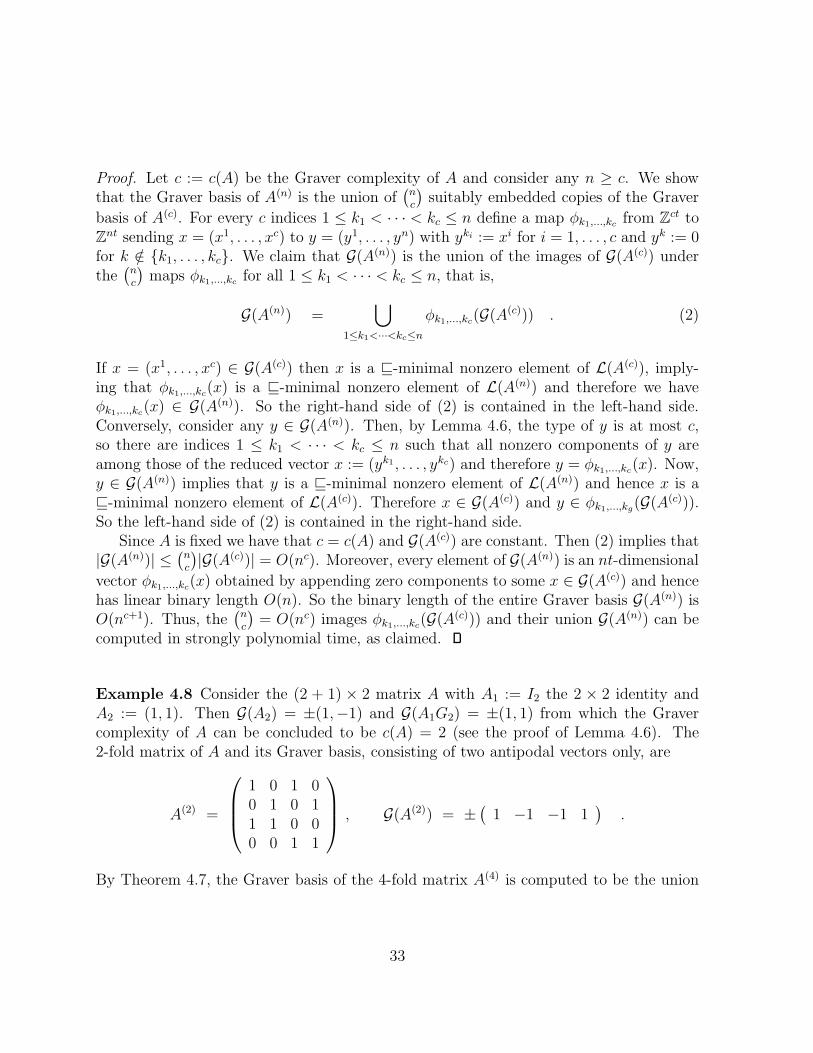
Proof. Let c := c(A) be the Graver complexity of A and consider any n ≥ c. We showthat the Graver basis of A(n) is the union of

(

n

c

)

suitably embedded copies of the Graver

basis of A(c). For every c indices 1 ≤ k1 < · · · < kc ≤ n define a map φk1,...,kcfrom Z

ct toZ

nt sending x = (x1, . . . , xc) to y = (y1, . . . , yn) with yki := xi for i = 1, . . . , c and yk := 0for k /∈ {k1, . . . , kc}. We claim that G(A(n)) is the union of the images of G(A(c)) underthe

(

n

c

)

maps φk1,...,kcfor all 1 ≤ k1 < · · · < kc ≤ n, that is,

G(A(n)) =⋃

1≤k1<···<kc≤n

φk1,...,kc(G(A(c))) . (2)

If x = (x1, . . . , xc) ∈ G(A(c)) then x is a ⊑-minimal nonzero element of L(A(c)), imply-ing that φk1,...,kc

(x) is a ⊑-minimal nonzero element of L(A(n)) and therefore we haveφk1,...,kc

(x) ∈ G(A(n)). So the right-hand side of (2) is contained in the left-hand side.Conversely, consider any y ∈ G(A(n)). Then, by Lemma 4.6, the type of y is at most c,so there are indices 1 ≤ k1 < · · · < kc ≤ n such that all nonzero components of y areamong those of the reduced vector x := (yk1, . . . , ykc) and therefore y = φk1,...,kc

(x). Now,y ∈ G(A(n)) implies that y is a ⊑-minimal nonzero element of L(A(n)) and hence x is a⊑-minimal nonzero element of L(A(c)). Therefore x ∈ G(A(c)) and y ∈ φk1,...,kg

(G(A(c))).So the left-hand side of (2) is contained in the right-hand side.

Since A is fixed we have that c = c(A) and G(A(c)) are constant. Then (2) implies that|G(A(n))| ≤

(

n

c

)

|G(A(c))| = O(nc). Moreover, every element of G(A(n)) is an nt-dimensional

vector φk1,...,kc(x) obtained by appending zero components to some x ∈ G(A(c)) and hence

has linear binary length O(n). So the binary length of the entire Graver basis G(A(n)) isO(nc+1). Thus, the

(

n

c

)

= O(nc) images φk1,...,kc(G(A(c))) and their union G(A(n)) can be

computed in strongly polynomial time, as claimed.

Example 4.8 Consider the (2 + 1) × 2 matrix A with A1 := I2 the 2 × 2 identity andA2 := (1, 1). Then G(A2) = ±(1,−1) and G(A1G2) = ±(1, 1) from which the Gravercomplexity of A can be concluded to be c(A) = 2 (see the proof of Lemma 4.6). The2-fold matrix of A and its Graver basis, consisting of two antipodal vectors only, are

A(2) =

1 0 1 00 1 0 11 1 0 00 0 1 1

, G(A(2)) = ±(

1 −1 −1 1)

.

By Theorem 4.7, the Graver basis of the 4-fold matrix A(4) is computed to be the union

33

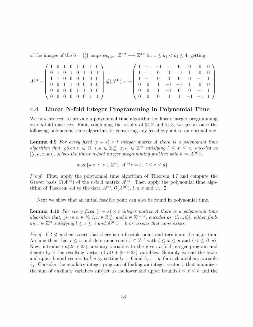
of the images of the 6 =(

42

)

maps φk1,k2: Z

2·2 −→ Z4·2 for 1 ≤ k1 < k2 ≤ 4, getting

A(4) =

1 0 1 0 1 0 1 00 1 0 1 0 1 0 11 1 0 0 0 0 0 00 0 1 1 0 0 0 00 0 0 0 1 1 0 00 0 0 0 0 0 1 1

,G(A(4)) = ±

1 −1 −1 1 0 0 0 01 −1 0 0 −1 1 0 01 −1 0 0 0 0 −1 10 0 1 −1 −1 1 0 00 0 1 −1 0 0 −1 10 0 0 0 1 −1 −1 1

.

4.4 Linear N-fold Integer Programming in Polynomial Time

We now proceed to provide a polynomial time algorithm for linear integer programmingover n-fold matrices. First, combining the results of §4.2 and §4.3, we get at once thefollowing polynomial time algorithm for converting any feasible point to an optimal one.

Lemma 4.9 For every fixed (r + s) × t integer matrix A there is a polynomial timealgorithm that, given n ∈ N, l, u ∈ Z

nt∞, x, w ∈ Z

nt satisfying l ≤ x ≤ u, encoded as[〈l, u, x, w〉], solves the linear n-fold integer programming problem with b := A(n)x,

max {wz : z ∈ Znt, A(n)z = b, l ≤ z ≤ u} .

Proof. First, apply the polynomial time algorithm of Theorem 4.7 and compute theGraver basis G(A(n)) of the n-fold matrix A(n). Then apply the polynomial time algo-rithm of Theorem 4.4 to the data A(n), G(A(n)), l, u, x and w.

Next we show that an initial feasible point can also be found in polynomial time.

Lemma 4.10 For every fixed (r + s) × t integer matrix A there is a polynomial timealgorithm that, given n ∈ N, l, u ∈ Z

nt∞, and b ∈ Z

r+ns, encoded as [〈l, u, b〉], either findsan x ∈ Z

nt satisfying l ≤ x ≤ u and A(n)x = b or asserts that none exists.

Proof. If l 6≤ u then assert that there is no feasible point and terminate the algorithm.Assume then that l ≤ u and determine some x ∈ Z

nt with l ≤ x ≤ u and 〈x〉 ≤ 〈l, u〉.Now, introduce n(2r + 2s) auxiliary variables to the given n-fold integer program anddenote by x the resulting vector of n(t + 2r + 2s) variables. Suitably extend the lowerand upper bound vectors to l, u by setting lj := 0 and uj := ∞ for each auxiliary variablexj . Consider the auxiliary integer program of finding an integer vector x that minimizes

the sum of auxiliary variables subject to the lower and upper bounds l ≤ x ≤ u and the

34

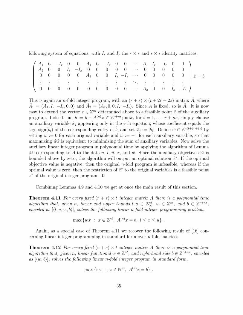
following system of equations, with Ir and Is the r × r and s × s identity matrices,

A1 Ir −Ir 0 0 A1 Ir −Ir 0 0 · · · A1 Ir −Ir 0 0A2 0 0 Is −Is 0 0 0 0 0 · · · 0 0 0 0 00 0 0 0 0 A2 0 0 Is −Is · · · 0 0 0 0 0...

......

......

......

......

.... . .

......

......

...0 0 0 0 0 0 0 0 0 0 · · · A2 0 0 Is −Is

x = b.

This is again an n-fold integer program, with an (r + s) × (t + 2r + 2s) matrix A, whereA1 = (A1, Ir,−Ir, 0, 0) and A2 = (A2, 0, 0, Is,−Is). Since A is fixed, so is A. It is noweasy to extend the vector x ∈ Z

nt determined above to a feasible point x of the auxiliaryprogram. Indeed, put b := b − A(n)x ∈ Z

r+ns; now, for i = 1, . . . , r + ns, simply choosean auxiliary variable xj appearing only in the i-th equation, whose coefficient equals the

sign sign(bi) of the corresponding entry of b, and set xj := |bi|. Define w ∈ Zn(t+2r+2s) by

setting w := 0 for each original variable and w := −1 for each auxiliary variable, so thatmaximizing wx is equivalent to minimizing the sum of auxiliary variables. Now solve theauxiliary linear integer program in polynomial time by applying the algorithm of Lemma4.9 corresponding to A to the data n, l, u, x, and w. Since the auxiliary objective wx isbounded above by zero, the algorithm will output an optimal solution x∗. If the optimalobjective value is negative, then the original n-fold program is infeasible, whereas if theoptimal value is zero, then the restriction of x∗ to the original variables is a feasible pointx∗ of the original integer program.

Combining Lemmas 4.9 and 4.10 we get at once the main result of this section.

Theorem 4.11 For every fixed (r + s) × t integer matrix A there is a polynomial timealgorithm that, given n, lower and upper bounds l, u ∈ Z

nt∞, w ∈ Z

nt, and b ∈ Zr+ns,

encoded as [〈l, u, w, b〉], solves the following linear n-fold integer programming problem,

max {wx : x ∈ Znt, A(n)x = b, l ≤ x ≤ u} .

Again, as a special case of Theorem 4.11 we recover the following result of [16] con-cerning linear integer programming in standard form over n-fold matrices.

Theorem 4.12 For every fixed (r + s) × t integer matrix A there is a polynomial timealgorithm that, given n, linear functional w ∈ Z

nt, and right-hand side b ∈ Zr+ns, encoded

as [〈w, b〉], solves the following linear n-fold integer program in standard form,

max {wx : x ∈ Nnt, A(n)x = b} .

35

4.5 Some Applications

4.5.1 Three-Way Line-Sum Transportation Problems

Transportation problems form a very important class of discrete optimization problemsstudied extensively in the operations research and mathematical programming literature,see e.g. [6, 42, 43, 53, 60, 62] and the references therein. We will discuss this class ofproblem and its applications to secure statistical data disclosure in more detail in §6.

It is well known that 2-way transportation problems are polynomial time solvable,since they can be encoded as linear integer programs over totally unimodular systems.However, already 3-way transportation problem are much more complicated. Considerthe following 3-way transportation problem over p× q × n tables with all line-sums fixed,

max{wx : x ∈ Np×q×n ,

∑

i

xi,j,k = zj,k ,∑

j

xi,j,k = vi,k ,∑

k

xi,j,k = ui,j } .

The data for the problem consist of given integer numbers (lines-sums) ui,j, vi,k, zj,k fori = 1, . . . , p, j = 1, . . . , q, k = 1, . . . , n, and a linear functional given by a p× q×n integerarray w representing the transportation profit per unit on each cell. The problem is tofind a transportation, that is, a p × q × n nonnegative integer table x satisfying the linesum constraints, which attains maximum profit wx =

∑p

i=1

∑q

j=1

∑n

k=1 wi,j,kxi,j,k.When at least two of the table sides, say p, q, are variable part of the input, and even

when the third side is fixed and as small as n = 3, this problem is already universal forinteger programming in a very strong sense [13, 15], and in particular is NP-hard [12];this will be discussed in detail and proved in §6. We now show that in contrast, whentwo sides, say p, q, are fixed (but arbitrary), and one side n is variable, then the 3-waytransportation problem over such long tables is an n-fold integer programming problemand therefore, as a consequence of Theorem 4.12, can be solved is polynomial time.

Corollary 4.13 For every fixed p and q there is a polynomial time algorithm that, givenn, integer profit array w ∈ Z

p×q×n, and line-sums u ∈ Zp×q, v ∈ Z

p×n and z ∈ Zq×n,

encoded as [〈w, u, v, z〉], solves the integer 3-way line-sum transportation problem

max{wx : x ∈ Np×q×n ,

∑

i

xi,j,k = zj,k ,∑

j

xi,j,k = vi,k ,∑

k

xi,j,k = ui,j } .

Proof. Re-index p × q × n arrays as x = (x1, . . . , xn) with each component indexed asxk := (xk

i,j) := (x1,1,k, . . . , xp,q,k) suitably indexed as a pq vector representing the k-thlayer of x. Put r := t := pq and s := p + q, and let A be the (r + s) × t matrix withA1 := Ipq the pq×pq identity and with A2 the (p+q)×pq matrix of equations of the usual2-way transportation problem for p× q arrays. Re-arrange the given line-sums in a vectorb := (b0, b1, . . . , bn) ∈ Z

r+ns with b0 := (ui,j) and bk := ((vi,k), (zj,k)) for k = 1, . . . , n.

36

This translates the given 3-way transportation problem into an n-fold integer pro-gramming problem in standard form,

max {wx : x ∈ Nnt, A(n)x = b} ,

where the equations A1(∑n

k=1 xk) = b0 represent the constraints∑

k xi,j,k = ui,j of allline-sums where summation over layers occurs, and the equations A2x

k = bk for k =1, . . . , n represent the constraints

∑

i xi,j,k = zj,k and∑

j xi,j,k = vi,k of all line-sumswhere summations are within a single layer at a time.

Using the algorithm of Theorem 4.12, this n-fold integer program, and hence the given3-way transportation problem, can be solved in polynomial time.

Example 4.14 We demonstrate the encoding of the p× q×n transportation problem asan n-fold integer program as in the proof of Corollary 4.13 for p = q = 3 (smallest casewhere the problem is genuinely 3-dimensional). Here we put r := t := 9, s := 6, write

xk := (x1,1,k, x1,2,k, x1,3,k, x2,1,k, x2,2,k, x2,3,k, x3,1,k, x3,2,k, x3,3,k) , k = 1, . . . , n ,

and let the (9 + 6) × 9 matrix A consist of A1 = I9 the 9 × 9 identity matrix and

A2 :=

1 1 1 0 0 0 0 0 00 0 0 1 1 1 0 0 00 0 0 0 0 0 1 1 11 0 0 1 0 0 1 0 00 1 0 0 1 0 0 1 00 0 1 0 0 1 0 0 1

.

Then the corresponding n-fold integer program encodes the 3 × 3 × n transportationproblem as desired. Already for this case, of 3× 3× n tables, the only known polynomialtime algorithm for the transportation problem is the one underlying Corollary 4.13.

Corollary 4.13 has a very broad generalization to multiway transportation problemsover long k-way tables of any dimension k; this will be discussed in detail in §6.

4.5.2 Packing Problems and Cutting-Stock

We consider the following rather general class of packing problems which concern max-imum utility packing of many items of several types in various bins subject to weightconstraints. More precisely, the data is as follows. There are t types of items. Each itemof type j has integer weight vj . There are nj items of type j to be packed. There are

37

n bins. The weight capacity of bin k is an integer uk. Finally, there is a utility matrixw ∈ Z

t×n where wj,k is the utility of packing one item of type j in bin k. The problem is tofind a feasible packing of maximum total utility. By incrementing the number t of typesby 1 and suitably augmenting the data, we may assume that the last type t represents“slack items” which occupy the unused capacity in each bin, where the weight of eachslack item is 1, the utility of packing any slack item in any bin is 0, and the number ofslack items is the total residual weight capacity nt :=

∑n

k=1 uk −∑t−1

j=1 njvj. Let x ∈ Nt×n

be a variable matrix where xj,k represents the number of items of type j to be packed inbin k. Then the packing problem becomes the following linear integer program,

max{wx : x ∈ Nt×n ,

∑

j

vjxj,k = uk ,∑

k

xj,k = nj } .

We now show that this is in fact an n-fold integer programming problem and therefore,as a consequence of Theorem 4.12, can be solved is polynomial time. While the number tof types and type weights vj are fixed, which is natural in many bin packing applications,the numbers nj of items of each type and the bin capacities uk may be very large.

Corollary 4.15 For every fixed number t of types and integer type weights v1, . . . , vt,there is a polynomial time algorithm that, given n bins, integer item numbers n1, . . . , nt,integer bin capacities u1, . . . , un, and t × n integer utility matrix w, encoded as[〈n1, . . . , nt, u1, . . . , un, w〉], solves the following integer bin packing problem,

max{wx : x ∈ Nt×n ,

∑

j

vjxj,k = uk ,∑

k

xj,k = nj } .

Proof. Re-index the variable matrix as x = (x1, . . . , xn) with xk := (xk1, . . . , x

kt ) where xk

j

represents the number of items of type j to be packed in bin k for al j and k. Let A be the(t+1)×t matrix with A1 := It the t×t identity and with A2 := (v1, . . . , vt) a single row. Re-arrange the given item numbers and bin capacities in a vector b := (b0, b1, . . . , bn) ∈ Z

t+n

with b0 := (n1, . . . , nt) and bk := uk for all k. This translates the bin packing probleminto an n-fold integer programming problem in standard form,

max {wx : x ∈ Nnt, A(n)x = b} ,

where the equations A1(∑n

k=1 xk) = b0 represent the constraints∑

k xj,k = nj assuringthat all items of each type are packed, and the equations A2x

k = bk for k = 1, . . . , nrepresent the constraints

∑

j vjxj,k = uk assuring that the weight capacity of each bin isnot exceeded (in fact, the slack items make sure each bin is perfectly packed).

Using the algorithm of Theorem 4.12, this n-fold integer program, and hence the giveninteger bin packing problem, can be solved in polynomial time.

38

Example 4.16 (cutting-stock problem). This is a classical manufacturing problem[27], where the usual setup is as follows: a manufacturer produces rolls of material (such asscotch-tape or band-aid) in one of t different widths v1, . . . , vt. The rolls are cut out fromstandard rolls of common large width u. Given orders by customers for nj rolls of widthvj , the problem facing the manufacturer is to meet the orders using the smallest possiblenumber of standard rolls. This can be cast as a bin packing problem as follows. Rollsof width vj become items of type j to be packed. Standard rolls become identical bins,of capacity uk := u each, where the number of bins is set to be n :=

∑t

j=1⌈nj/⌊u/vj⌋⌉which is sufficient to accommodate all orders. The utility of each roll of width vj is setto be its width negated wj,k := −vj regardless of the standard roll k from which it is cut(paying for the width it takes). Introduce a new roll width v0 := 1, where rolls of thatwidth represent “slack rolls” which occupy the unused width of each standard roll, withutility w0,k := −1 regardless of the standard roll k from which it is cut (paying for theunused width it represents), with the number of slack rolls set to be the total residualwidth n0 := nu −

∑t

j=1 njvj . Then the cutting-stock problem becomes a bin packingproblem and therefore, by Corollary 4.15, for every fixed t and fixed roll widths v1, . . . , vt,it is solvable in time polynomial in

∑t

j=1⌈nj/⌊u/vj⌋⌉ and 〈n1, . . . , nt, u〉.One common approach to the cutting-stock problem uses so-called cutting patterns,

which are feasible solutions of the knapsack problem {y ∈ Nt :∑t

j=1 vjyj ≤ u}. This isuseful when the common width u of the standard rolls is of the same order of magnitudeas the demand role widths vj . However, when u is much larger than the vj , the numberof cutting patterns becomes prohibitively large to handle. But then the values ⌊u/vj⌋ arelarge and hence n :=

∑t

j=1⌈nj/⌊u/vj⌋⌉ is small, in which case the solution through thealgorithm of Corollary 4.15 becomes particularly appealing.

39

5 Convex Integer Programming

In this section we discuss convex integer programming. In particular, we extend the theoryof §4 and show that convex n-fold integer programming is polynomial time solvable aswell. In §5.1 we discuss convex integer programming over totally unimodular matrices.In §5.2 we show the applicability of Graver bases to convex integer programming. In §5.3we combine Theorem 2.4, the results of §4, and the preparatory facts from §§5.2, andprove the main result of this section, asserting that convex n-fold integer programming ispolynomial time solvable. We conclude with some applications in §5.4.

As in §4, the feasible set S is presented as the set of integer points satisfying anexplicitly given system of linear inequalities, given in one of the forms

S := {x ∈ Nn : Ax = b} or S := {x ∈ Z

n : Ax = b, l ≤ x ≤ u} ,

with matrix A ∈ Zm×n, right-hand side b ∈ Z

m, and lower and upper bounds l, u ∈ Zn∞.

As demonstrated in §1.1, if the polyhedron P := {x ∈ Rn : Ax = b, l ≤ x ≤ u}

is unbounded then the convex integer programming problem with an oracle presentedconvex functional is rather hopeless. Therefore, an algorithm that solves the convexinteger programming problem should either return an optimal solution, or assert that theprogram is infeasible, or assert that the underlying polyhedron is unbounded.

Nonetheless, we do allow the lower and upper bounds l, u to lie in Zn∞ rather than

Zn, since often the polyhedron is bounded even though the variables are not bounded

explicitly (for instance, if each variable is bounded below only, and appears in some equa-tion all of whose coefficients are positive). This results in broader formulation flexibility.Furthermore, in the next subsections we prove auxiliary lemmas asserting that certainsets cover all edge-directions of relevant polyhedra, which do hold also in the unboundedcase. So we now extend the notion of edge-directions, defined in §2.1 for polytopes, topolyhedra. A direction of an edge (1-dimensional face) e of a polyhedron P is any nonzeroscalar multiple of y−x where x, y are any two distinct points in e. As before, a set coversall edge-directions of P if it contains a direction of each edge of P .

5.1 Convex Integer Programming over Totally Unimodular Sys-tems

A matrix A is totally unimodular if the determinant of every square submatrix of A lies in{−1, 0, 1}. Such matrices arise naturally in network flows, ordinary (2-way) transportationproblems, and many other situations. A fundamental result in integer programming [37]asserts that polyhedra defined by totally unimodular matrices are integer. More precisely,if A is an m × n totally unimodular matrix, l, u ∈ Z

n∞, and b ∈ Z

m, then

PI := conv{x ∈ Zn : Ax = b, l ≤ x ≤ u} = {x ∈ R

n : Ax = b, l ≤ x ≤ u} := P ,

40

that is, the underlying polyhedron P coincides with its integer hull PI . This has twoconsequences useful in facilitating the solution of the corresponding convex integer pro-gramming problem via the algorithm of Theorem 2.4. First, the corresponding linearinteger programming problem can be solved by linear programming over P in polynomialtime. Second, a set covering all edge-directions of the implicitly given integer hull PI ,which is typically very hard to determine, is obtained here as a set covering all edge-directions of P which is explicitly given and hence easier to determine.

We now describe a well known property of polyhedra of the above form. A circuit ofa matrix A ∈ Z

m×n is a nonzero primitive minimal support element of L(A). So a circuitis a nonzero c ∈ Z

n satisfying Ac = 0, whose entries are relatively prime integers, suchthat no nonzero c′ with Ac′ = 0 has support strictly contained in the support of c.

Lemma 5.1 For every A ∈ Zm×n, l, u ∈ Z

n∞, and b ∈ Z

m, the set of circuits of A coversall edge-directions of the polyhedron P := {x ∈ R

n : Ax = b, l ≤ x ≤ u}.

Proof. Consider any edge e of P . Pick two distinct points x, y ∈ e and set g := y − x.Then Ag = 0 and therefore, as can be easily proved by induction on |supp(g)|, there isa finite decomposition g =

∑

i αici with αi positive real number and ci circuit of A suchthat αici ⊑ g for all i, where ⊑ is the natural extension from Z

n to Rn of the partial order

defined in §4.2. We claim that x + αici ∈ P for all i. Indeed, ci being a circuit impliesA(x + αici) = Ax = b; and l ≤ x, x + g ≤ u and αici ⊑ g imply l ≤ x + αici ≤ u.

Now let w ∈ Rn be a linear functional uniquely maximized over P at the edge e. Then

wαici = w(x + αici) − wx ≤ 0 for all i. But∑

(wαici) = wg = wy − wx = 0, implyingthat in fact wαici = 0 and hence x + αici ∈ e for all i. This implies that each ci is adirection of e (in fact, all ci are the same and g is a multiple of some circuit).

Combining Theorem 2.4 and Lemma 5.1 we obtain the following statement.

Theorem 5.2 For every fixed d there is a polynomial time algorithm that, given m × ntotally unimodular matrix A, set C ⊂ Z

n containing all circuits of A, vectors l, u ∈ Zn∞,

b ∈ Zm, and w1, . . . , wd ∈ Z

n, and convex c : Rd −→ R presented by a comparison oracle,

encoded as [〈A, C, l, u, b, w1, . . . , wd〉], solves the convex integer program

max {c(w1x, . . . , wdx) : x ∈ Zn, Ax = b, l ≤ x ≤ u} .

Proof. First, check in polynomial time using linear programming whether the objectivefunction of any of the following 2n linear programs is unbounded,

max {±yi : y ∈ P}, i = 1, . . . , n, P := {y ∈ Rn : Ay = b, l ≤ y ≤ u} .

41

If any is unbounded then terminate, asserting that P is unbounded. Otherwise, let ρ bethe least integer upper bound on the absolute value of all optimal objective values. ThenP ⊆ [−ρ, ρ]n and S := {y ∈ Z

n : Ay = b, l ≤ y ≤ u} ⊂ P is finite of radius ρ(S) ≤ ρ. Infact, since A is totally unimodular, PI = P = conv(S) and hence ρ(S) = ρ. Moreover, byCramer’s rule, 〈ρ〉 is polynomially bounded in 〈A, l, u, x〉.

Now, since A is totally unimodular, using linear programming over PI = P we cansimulate in polynomial time a linear discrete optimization oracle for S. By Lemma5.1, the given set C, which contains all circuits of A, also covers all edge-directions ofconv(S) = PI = P . Therefore we can apply the algorithm of Theorem 2.4 and solve thegiven convex n-fold integer programming problem in polynomial time.

While the number of circuits of an m × n matrix A can be as large as 2(

n

m+1

)

andhence exponential in general, it is nonetheless relatively small in that it is bounded interms of m and n only and is independent of the matrix A itself. Furthermore, it mayhappen that the number of circuits is much smaller than the upper bound 2

(

n

m+1

)

. Also,if in a class of matrices, m grows slowly in terms of n, say m = O(log n), then this boundis subexponential. In such situations, the above theorem may provide a good strategy forsolving convex integer programming over totally unimodular systems.

5.2 Graver Bases and Convex Integer Programming

We now extend the statements of §5.1 about totally unimodular matrices to arbitraryinteger matrices. The next lemma shows that the Graver basis of any integer matrixcovers all edge-directions of the integer hulls of polyhedra defined by that matrix.

Lemma 5.3 For every A ∈ Zm×n, l, u ∈ Z

n∞, and b ∈ Z

m, the Graver basis G(A) of Acovers all edge-directions of the polyhedron PI := conv{x ∈ Z

n : Ax = b, l ≤ x ≤ u}.

Proof. Consider any edge e of PI and pick two distinct points x, y ∈ e ∩ Zn. Then

g := y−x is in L(A) \ {0}. Therefore, by Lemma 4.2, there is a conformal sum g =∑

i hi

with hi ∈ G(A) for all i. We claim that x + hi ∈ PI for all i. Indeed, first note thathi ∈ G(A) ⊂ L(A) implies Ahi = 0 and hence A(x + hi) = Ax = b; and second note thatl ≤ x, x + g ≤ u and hi ⊑ g imply that l ≤ x + hi ≤ u.

Now let w ∈ Zn be a linear functional uniquely maximized over PI at the edge e. Then

whi = w(x + hi) − wx ≤ 0 for all i. But∑

(whi) = wg = wy − wx = 0, implying that infact whi = 0 and hence x + hi ∈ e for all i. Therefore each hi is a direction of e (in fact,all hi are the same and g is a multiple of some Graver basis element).

Combining Theorems 2.4 and 4.4 and Lemma 5.3 we obtain the following statement.

42

Theorem 5.4 For every fixed d there is a polynomial time algorithm that, given in-teger m × n matrix A, its Graver basis G(A), l, u ∈ Z

n∞, x ∈ Z

n with l ≤ x ≤ u,w1, . . . , wd ∈ Z

n, and convex c : Rd −→ R presented by a comparison oracle, encoded as

[〈A,G(A), l, u, x, w1, . . . , wd〉], solves the convex integer program with b := Ax,

max {c(w1z, . . . , wdz) : z ∈ Zn, Az = b, l ≤ z ≤ u} .

Proof. First, check in polynomial time using linear programming whether the objectivefunction of any of the following 2n linear programs is unbounded,

max {±yi : y ∈ P}, i = 1, . . . , n, P := {y ∈ Rn : Ay = b, l ≤ y ≤ u} .

If any is unbounded then terminate, asserting that P is unbounded. Otherwise, let ρ bethe least integer upper bound on the absolute value of all optimal objective values. ThenP ⊆ [−ρ, ρ]n and S := {y ∈ Z

n : Ay = b, l ≤ y ≤ u} ⊂ P is finite of radius ρ(S) ≤ ρ.Moreover, by Cramer’s rule, 〈ρ〉 is polynomially bounded in 〈A, l, u, x〉.

Using the given Graver basis and applying the algorithm of Theorem 4.4 we cansimulate in polynomial time a linear discrete optimization oracle for S. Furthermore,by Lemma 5.3, the given Graver basis covers all edge-directions of the integer hullPI := conv{y ∈ Z

n : Ay = b, l ≤ y ≤ u} = conv(S). Therefore we can apply the al-gorithm of Theorem 2.4 and solve the given convex program in polynomial time.

5.3 Convex N-fold Integer Programming in Polynomial Time

We now extend the result of Theorem 4.11 and show that convex integer programmingproblems over n-fold systems can be solved in polynomial time as well. As explained inthe beginning of this section, the algorithm either returns an optimal solution, or assertsthat the program is infeasible, or asserts that the underlying polyhedron is unbounded.

Theorem 5.5 For every fixed d and fixed (r + s)× t integer matrix A there is a polyno-mial time algorithm that, given n, lower and upper bounds l, u ∈ Z

nt∞, w1, . . . , wd ∈ Z

nt,b ∈ Z

r+ns, and convex functional c : Rd −→ R presented by a comparison oracle, encoded

as [〈l, u, w1, . . . , wd, b〉], solves the convex n-fold integer programming problem

max {c(w1x, . . . , wdx) : x ∈ Znt, A(n)x = b, l ≤ x ≤ u} .

Proof. First, check in polynomial time using linear programming whether the objectivefunction of any of the following 2nt linear programs is unbounded,

max {±yi : y ∈ P}, i = 1, . . . , nt, P := {y ∈ Rnt : A(n)y = b, l ≤ y ≤ u} .

43

If any is unbounded then terminate, asserting that P is unbounded. Otherwise, let ρ bethe least integer upper bound on the absolute value of all optimal objective values. ThenP ⊆ [−ρ, ρ]nt and S := {y ∈ Z

nt : A(n)y = b, l ≤ y ≤ u} ⊂ P is finite of radius ρ(S) ≤ ρ.Moreover, by Cramer’s rule, 〈ρ〉 is polynomially bounded in n and 〈l, u, b〉.

Using the algorithm of Theorem 4.11 we can simulate in polynomial time a lineardiscrete optimization oracle for S. Also, using the algorithm of Theorem 4.7 we cancompute in polynomial time the Graver basis G(A(n)) which, by Lemma 5.3, covers alledge-directions of PI := conv{y ∈ Z

nt : A(n)y = b, l ≤ y ≤ u} = conv(S). Thereforewe can apply the algorithm of Theorem 2.4 and solve the given convex n-fold integerprogramming problem in polynomial time.

Again, as a special case of Theorem 5.5 we recover the following result of [17] concern-ing convex integer programming in standard form over n-fold matrices.

Theorem 5.6 For every fixed d and fixed (r + s) × t integer matrix A there is a poly-nomial time algorithm that, given n, linear functionals w1, . . . , wd ∈ Z

nt, right-hand sideb ∈ Z

r+ns, and convex functional c : Rd −→ R presented by a comparison oracle, encoded

as [〈w1, . . . , wd, b〉], solves the convex n-fold integer program in standard form

max {c(w1x, . . . , wdx) : x ∈ Nnt, A(n)x = b} .

5.4 Some Applications

5.4.1 Transportation Problems and Packing Problems

Theorems 5.5 and 5.6 generalize Theorems 4.11 and 4.12 by broadly extending the classof objective functions that can be maximized in polynomial time over n-fold systems.Therefore all applications discussed in §4.5 automatically extend accordingly.

First, we have the following analog of Corollary 4.13 for the convex integer trans-portation problem over long 3-way tables. This has a very broad further generalization tomultiway transportation problems over long k-way tables of any dimension k, see §6.

Corollary 5.7 For every fixed d, p, q there is a polynomial time algorithm that, givenn, arrays w1, . . . , wd ∈ Z

p×q×n, line-sums u ∈ Zp×q, v ∈ Z

p×n and z ∈ Zq×n, and convex

functional c : Rd −→ R presented by a comparison oracle, encoded as [〈w1, . . . , wd, u, v, z〉],

solves the convex integer 3-way line-sum transportation problem

max{ c(w1x, . . . , wdx) : x ∈ Np×q×n ,

∑

i

xi,j,k = zj,k ,∑

j

xi,j,k = vi,k ,∑

k

xi,j,k = ui,j } .

44

Second, we have the following analog of Corollary 4.15 for convex bin packing.

Corollary 5.8 For every fixed d, number of types t, and type weights v1, . . . , vt ∈ Z, thereis a polynomial time algorithm that, given n bins, item numbers n1, . . . , nt ∈ Z, bin capaci-ties u1, . . . , un ∈ Z, utility matrices w1, . . . , wd ∈ Z

t×n, and convex functional c : Rd −→ R

presented by a comparison oracle, encoded as [〈n1, . . . , nt, u1, . . . , un, w1, . . . , wd〉], solvesthe convex integer bin packing problem,

max{ c(w1x, . . . , wdx) : x ∈ Nt×n ,

∑

j

vjxj,k = uk ,∑

k

xj,k = nj } .

5.4.2 Vector Partitioning and Clustering

The vector partition problem concerns the partitioning of n items among p players tomaximize social value subject to constraints on the number of items each player canreceive. More precisely, the data is as follows. With each item i is associated a vectorvi ∈ Z

k representing its utility under k criteria. The utility of player h under orderedpartition π = (π1, . . . , πp) of the set of items {1, . . . , n} is the sum vπ

h :=∑

i∈πhvi of

utility vectors of items assigned to h under π. The social value of π is the balancingc(vπ

1,1, . . . , vπ1,k, . . . , v

πp,1, . . . , v

πp,k) of the player utilities, where c is a convex functional on

Rpk. In the constrained version, the partition must be of a given shape, i.e. the number

|πh| of items that player h gets is required to be a given number λh (with∑

λh = n). Inthe unconstrained version, there is no restriction on the number of items per player.

Vector partition problems have applications in diverse areas such as load balancing,circuit layout, ranking, cluster analysis, inventory, and reliability, see e.g. [7, 9, 25, 39, 50]and the references therein. Here is a typical example.

Example 5.9 (minimal variance clustering). This problem has numerous applica-tions in the analysis of statistical data: given n observed points v1, . . . , vn in k-space,group them into p clusters π1, . . . , πp that minimize the sum of cluster variances given by

p∑

h=1

1

|πh|

∑

i∈πh

||vi − (1

|πh|

∑

i∈πh

vi)||2 .

Consider instances where there are n = pm points and the desired clustering is balanced,that is, the clusters should have equal size m. Suitable manipulation of the sum ofvariances expression above shows that the problem is equivalent to a constrained vectorpartition problem, where λh = m for all h, and where the convex functional c : R

pk −→ R

(to be maximized) is the Euclidean norm squared, given by

c(z) = ||z||2 =

p∑

h=1

k∑

i=1

|zh,i|2 .

45

If either the number of criteria k or the number of players p is variable, the partitionproblem is intractable since it instantly captures NP-hard problems [39]. When both k, pare fixed, both the constrained and unconstrained versions of the vector partition problemare polynomial time solvable [39, 50]. We now show that vector partition problems (eitherconstrained or unconstrained) are in fact convex n-fold integer programming problems andtherefore, as a consequence of Theorem 5.6, can be solved is polynomial time.

Corollary 5.10 For every fixed number p of players and number k of criteria, there is apolynomial time algorithm that, given n, item vectors v1, . . . , vn ∈ Z

k, λ1, . . . , λp ∈ N,and convex functional c : R

pk −→ R presented by a comparison oracle, encoded as[〈v1, . . . , vn, λ1, . . . , λp〉], solves the constrained and unconstrained partitioning problems.

Proof. There is an obvious one-to-one correspondence between partitions and matricesx ∈ {0, 1}p×n with all column-sums equal to one, where partition π corresponds to thematrix x with xh,i = 1 if i ∈ πh and xh,i = 0 otherwise. Let d := pk and define d matriceswh,j ∈ Z

p×n by setting (wh,j)h,i := vi,j for all h = 1, . . . , p, i = 1, . . . , n and j = 1, . . . , k,and setting all other entries to zero. Then for any partition π and its corresponding matrixx we have vπ

h,j = wh,jx for all h = 1, . . . , p and j = 1, . . . , k. Therefore, the unconstrainedvector partition problem is the convex integer program

max{ c(w1,1x, . . . , wp,kx) : x ∈ Np×n ,

∑

h

xh,i = 1 } .

Suitably arranging the variables in a vector, this becomes a convex n-fold integer programwith a (0 + 1) × p defining matrix A, where A1 is empty and A2 := (1, . . . , 1).

Similarly, the constrained vector partition problem is the convex integer program

max{ c(w1,1x, . . . , wp,kx) : x ∈ Np×n ,

∑

h

xh,i = 1 ,∑

i

xh,i = λh } .

This again is a convex n-fold integer program, now with a (p + 1)× p defining matrix A,where now A1 := Ip is the p × p identity matrix and A2 := (1, . . . , 1) as before.

Using the algorithm of Theorem 5.6, this convex n-fold integer program, and hencethe given vector partition problem, can be solved in polynomial time.

46

6 Multiway Transportation Problems and Privacy in

Statistical Databases

Transportation problems form a very important class of discrete optimization problems.The feasible points in a transportation problem are the multiway tables (“contingencytables” in statistics) such that the sums of entries over some of their lower dimensionalsub-tables such as lines or planes (“margins” in statistics) are specified. Transportationproblems and their corresponding transportation polytopes have been used and studiedextensively in the operations research and mathematical programming literature, as wellas in the statistics literature in the context of secure statistical data disclosure and man-agement by public agencies, see [4, 6, 11, 18, 19, 42, 43, 53, 60, 62] and references therein.

In this section we completely settle the algorithmic complexity of treating multiwaytables and discuss the applications to transportation problems and secure statistical datadisclosure, as follows. After introducing some terminology in §6.1, we go on to describe,in §6.2, a universality result that shows that “short” 3-way r× c× 3 tables, with variablenumber r of rows and variable number c of columns but fixed small number 3 of layers(hence “short”), are universal in a very strong sense. In §6.3 we discuss the generalmultiway transportation problem. Using the results of §6.2 and the results on linearand convex n-fold integer programming from §4 and §5, we show that the transportationproblem is intractable for short 3-way r × c × 3 tables but polynomial time treatable for“long” (k + 1)-way m1 × · · · ×mk × n tables, with k and the sides m1, . . . , mk fixed (butarbitrary), and the number n of layers variable (hence “long”). In §6.4 we turn to discussdata privacy and security and consider the central problem of detecting entry uniquenessin tables with disclosed margins. We show that as a consequence of the results of §6.2and §6.3, and in analogy to the complexity of the transportation problem established in§6.3, the entry uniqueness problem is intractable for short 3-way r × c × 3 tables butpolynomial time decidable for long (k + 1)-way m1 × · · · × mk × n tables.

6.1 Tables and Margins

We start with some terminology on tables, margins and transportation polytopes.A k-way table is an m1 × · · · × mk array x = (xi1,...,ik) of nonnegative integers. A k-waytransportation polytope (or simply k-way polytope for brevity) is the set of all m1×· · ·×mk

nonnegative arrays x = (xi1,...,ik) such that the sums of the entries over some of their lowerdimensional sub-arrays (margins) are specified. More precisely, for any tuple (i1, . . . , ik)with ij ∈ {1, . . . , mj} ∪ {+}, the corresponding margin xi1,...,ik is the sum of entriesof x over all coordinates j with ij = +. The support of (i1, . . . , ik) and of xi1,...,ik isthe set supp(i1, . . . , ik) := {j : ij 6= +} of non-summed coordinates. For instance, ifx is a 4 × 5 × 3 × 2 array then it has 12 margins with support F = {1, 3} such as

47

x3,+,2,+ =∑5

i2=1

∑2i4=1 x3,i2,2,i4. A collection of margins is hierarchical if, for some family

F of subsets of {1, . . . , k}, it consists of all margins ui1,...,ik with support in F . In par-ticular, for any 0 ≤ h ≤ k, the collection of all h-margins of k-tables is the hierarchicalcollection with F the family of all h-subsets of {1, . . . , k}. Given a hierarchical collectionof margins ui1,...,ik supported on a family F of subsets of {1, . . . , k}, the correspondingk-way polytope is the set of nonnegative arrays with these margins,

TF :={

x ∈ Rm1×···×mk

+ : xi1,...,ik = ui1,...,ik , supp(i1, . . . , ik) ∈ F}

.

The integer points in this polytope are precisely the k-way tables with the given margins.

6.2 The Universality Theorem

We now describe the following universality result of [13, 15] which shows that, quiteremarkably, any rational polytope is a short 3-way r × c × 3 polytope with all line-sumsspecified. (In the terminology of §6.1 this is the r × c × 3 polytope TF of all 2-marginsfixed, supported on the family F = {{1, 2}, {1, 3}, {2, 3}}.) By saying that a polytopeP ⊂ R

p is representable as a polytope Q ⊂ Rq we mean in the strong sense that there is

an injection σ : {1, . . . , p} −→ {1, . . . , q} such that the coordinate-erasing projection

π : Rq −→ R

p : x = (x1, . . . , xq) 7→ π(x) = (xσ(1), . . . , xσ(p))

provides a bijection between Q and P and between the sets of integer points Q ∩ Zq and

P ∩ Zp. In particular, if P is representable as Q then P and Q are isomorphic in any

reasonable sense: they are linearly equivalent and hence all linear programming relatedproblems over the two are polynomial time equivalent; they are combinatorially equivalentand hence they have the same face numbers and facial structure; and they are integerequivalent and therefore all integer programming and integer counting related problemsover the two are polynomial time equivalent as well.

We provide only an outline of the proof of the following statement; complete detailsand more consequences of this theorem can be found in [13, 15].

Theorem 6.1 There is a polynomial time algorithm that, given A ∈ Zm×n and b ∈ Z

m,encoded as [〈A, b〉], produces r, c and line-sums u ∈ Z

r×c, v ∈ Zr×3 and z ∈ Z

c×3 such thatthe polytope P := {y ∈ R

n+ : Ay = b} is representable as the 3-way polytope

T := {x ∈ Rr×c×3+ :

∑

i

xi,j,k = zj,k ,∑

j

xi,j,k = vi,k ,∑

k

xi,j,k = ui,j } .

Proof. The construction proving the theorem consists of three polynomial time steps,each representing a polytope of a given format as a polytope of another given format.

48

First, we show that any P := {y ≥ 0 : Ay = b} with A, b integer can be representedin polynomial time as Q := {x ≥ 0 : Cx = d} with C matrix all entries of which arein {−1, 0, 1, 2}. This reduction of coefficients will enable the rest of the steps to run inpolynomial time. For each variable yj let kj := max{⌊log2 |ai,j|⌋ : i = 1, . . .m} be themaximum number of bits in the binary representation of the absolute value of any entry ai,j

of A. Introduce variables xj,0, . . . , xj,kj, and relate them by the equations 2xj,i−xj,i+1 = 0.

The representing injection σ is defined by σ(j) := (j, 0), embedding yj as xj,0. Consider

any term ai,j yj of the original system. Using the binary expansion |ai,j| =∑kj

s=0 ts2s with

all ts ∈ {0, 1}, we rewrite this term as ±∑kj

s=0 tsxj,s. It is not hard to verify that thisrepresents P as Q with defining {−1, 0, 1, 2}-matrix.

Second, we show that any Q := {y ≥ 0 : Ay = b} with A, b integer can be representedas a face F of a 3-way polytope with all plane-sums fixed, that is, a face of a 3-waypolytope TF of all 1-margins fixed, supported on the family F = {{1}, {2}, {3}}.

Since Q is a polytope and hence bounded, we can compute (using Cramer’s rule) aninteger upper bound U on the value of any coordinate yj of any y ∈ Q. Note also that aface of a 3-way polytope TF is the set of all x = (xi,j,k) with some entries forced to zero;these entries are termed “forbidden”, and the other entries are termed “enabled”.

For each variable yj, let rj be the largest between the sum of positive coefficients ofyj and the sum of absolute values of negative coefficients of yj over all equations,

rj := max

(

∑

k

{ak,j : ak,j > 0} ,∑

k

{|ak,j| : ak,j < 0}

)

.

Assume that A is of size m × n. Let r :=∑n

j=1 rj , R := {1, . . . , r}, h := m + 1 and

H := {1, . . . , h}. We now describe how to construct vectors u, v ∈ Zr, z ∈ Z

h, and a setE ⊂ R × R × H of triples - the enabled, non-forbidden, entries - such that the polytopeQ is represented as the face F of the corresponding 3-way polytope of r × r × h arrayswith plane-sums u, v, z and only entries indexed by E enabled,

F := { x ∈ Rr×r×h+ : xi,j,k = 0 for all (i, j, k) /∈ E , and

∑

i,j

xi,j,k = zk ,∑

i,k

xi,j,k = vj ,∑

j,k

xi,j,k = ui } .

We also indicate the injection σ : {1, . . . , n} −→ R×R×H giving the desired embeddingof coordinates yj as coordinates xi,j,k and the representation of Q as F .

Roughly, each equation k = 1, . . . , m is encoded in a “horizontal plane” R × R × {k}(the last plane R × R × {h} is included for consistency with its entries being “slacks”);and each variable yj, j = 1, . . . , n is encoded in a “vertical box” Rj × Rj × H , whereR =

⊎n

j=1 Rj is the natural partition of R with |Rj | = rj for all j = 1, . . . , n, that is, withRj := {1 +

∑

l<j rl, . . . ,∑

l≤j rl}.

49

Now, all “vertical” plane-sums are set to the same value U , that is, uj := vj := Ufor j = 1, . . . , r. All entries not in the union

⊎n

j=1 Rj × Rj × H of the variable boxeswill be forbidden. We now describe the enabled entries in the boxes; for simplicity wediscuss the box R1 × R1 × H , the others being similar. We distinguish between the twocases r1 = 1 and r1 ≥ 2. In the first case, R1 = {1}; the box, which is just the singleline {1} × {1} × H , will have exactly two enabled entries (1, 1, k+), (1, 1, k−) for suitablek+, k− to be defined later. We set σ(1) := (1, 1, k+), namely embed y1 = x1,1,k+ . We definethe complement of the variable y1 to be y1 := U −y1 (and likewise for the other variables).The vertical sums u, v then force y1 = U − y1 = U − x1,1,k+ = x1,1,k−, so the complementof y1 is also embedded. Next, consider the case r1 ≥ 2. For each s = 1, . . . , r1, the line{s}× {s}×H (respectively, {s}× {1 + (s mod r1)}×H) will contain one enabled entry(s, s, k+(s)) (respectively, (s, 1 + (s mod r1), k

−(s)). All other entries of R1 × R1 × Hwill be forbidden. Again, we set σ(1) := (1, 1, k+(1)), namely embed y1 = x1,1,k+(1); it isthen not hard to see that, again, the vertical sums u, v force xs,s,k+(s) = x1,1,k+(1) = y1 andxs,1+(s mod r1),k−(s) = U − x1,1,k+(1) = y1 for each s = 1, . . . , r1. Therefore, both y1 and y1

are each embedded in r1 distinct entries.We now encode the equations by defining the horizontal plane-sums z and the indices

k+(s), k−(s) above as follows. For k = 1, . . . , m, consider the k-th equation∑

j ak,jyj = bk. Define the index sets J+ := {j : ak,j > 0} and J− := {j : ak,j < 0}, andset zk := bk + U ·

∑

j∈J− |ak,j|. The last coordinate of z is set for consistency with u, v tobe zh = zm+1 := r · U −

∑m

k=1 zk. Now, with yj := U − yj the complement of variable yj

as above, the k-th equation can be rewritten as

∑

j∈J+

ak,jyj +∑

j∈J−

|ak,j|yj =n∑

j=1

ak,jyj + U ·∑

j∈J−

|ak,j| = bk + U ·∑

j∈J−

|ak,j| = zk.

To encode this equation, we simply “pull down” to the corresponding k-th horizontal planeas many copies of each variable yj or yj by suitably setting k+(s) := k or k−(s) := k. Bythe choice of rj there are sufficiently many, possibly with a few redundant copies whichare absorbed in the last hyperplane by setting k+(s) := m + 1 or k−(s) := m + 1. Thiscompletes the encoding and provides the desired representation.

Third, we show that any 3-way polytope with plane-sums fixed and entry bounds,

F := { y ∈ Rl×m×n+ :

∑

i,j

yi,j,k = ck ,∑

i,k

yi,j,k = bj ,∑

j,k

yi,j,k = ai , yi,j,k ≤ ei,j,k} ,

can be represented as a 3-way polytope with line-sums fixed (and no entry bounds),

T := { x ∈ Rr×c×3+ :

∑

I

xI,J,K = zJ,K ,∑

J

xI,J,K = vI,K ,∑

K

xI,J,K = uI,J } .

50

In particular, this implies that any face F of a 3-way polytope with plane-sums fixed canbe represented as a 3-way polytope T with line-sums fixed: forbidden entries are encodedby setting a “forbidding” upper-bound ei,j,k := 0 on all forbidden entries (i, j, k) /∈ E andan “enabling” upper-bound ei,j,k := U on all enabled entries (i, j, k) ∈ E. We describe thepresentation, but omit the proof that it is indeed valid; further details on this step canbe found in [12, 13, 15]. We give explicit formulas for uI,J , vI,K , zJ,K in terms of ai, bj , ck

and ei,j,k as follows. Put r := l · m and c := n + l + m. The first index I of each entryxI,J,K will be a pair I = (i, j) in the r-set

{(1, 1), . . . , (1, m), (2, 1), . . . , (2, m), . . . , (l, 1), . . . , (l, m)} .

The second index J of each entry xI,J,K will be a pair J = (s, t) in the c-set

{(1, 1), . . . , (1, n), (2, 1), . . . , (2, l), (3, 1), . . . , (3, m)} .

The last index K will simply range in the 3-set {1, 2, 3}. We represent F as T viathe injection σ given explicitly by σ(i, j, k) := ((i, j), (1, k), 1), embedding each variableyi,j,k as the entry x(i,j),(1,k),1. Let U now denote the minimal between the two valuesmax{a1, . . . , al} and max{b1, . . . , bm}. The line-sums (2-margins) are set to be

u(i,j),(1,t) = ei,j,t, u(i,j),(2,t) =

{

U if t = i,0 otherwise.

, u(i,j),(3,t) =

{

U if t = j,0 otherwise.

v(i,j),t =

U if t = 1,ei,j,+ if t = 2,U if t = 3.

, z(i,j),1 =

cj if i = 1,m · U − aj if i = 2,0 if i = 3.

z(i,j),2 =

e+,+,j − cj if i = 1,0 if i = 2,bj if i = 3.

, z(i,j),3 =

0 if i = 1,aj if i = 2,l · U − bj if i = 3.

.

Applying the first step to the given rational polytope P , applying the second step tothe resulting Q, and applying the third step to the resulting F , we get in polynomial timea 3-way r × c × 3 polytope T of all line-sums fixed representing P as claimed.

6.3 The Complexity of the Multiway Transportation Problem

We are now finally in position to settle the complexity of the general multiway transporta-tion problem. The data for the problem consists of: positive integers k (table dimension)and m1, . . . , mk (table sides); family F of subsets of {1, . . . , k} (supporting the hierar-chical collection of margins to be fixed); integer values ui1,...,ik for all margins supported

51

on F ; and integer “profit” m1 × · · · × mk array w. The transportation problem is tofind an m1 × · · · × mk table having the given margins and attaining maximum profit, orassert than none exists. Equivalently, it is the linear integer programming problem ofmaximizing the linear functional defined by w over the transportation polytope TF ,

max{

wx : x ∈ Nm1×···×mk : xi1,...,ik = ui1,...,ik , supp(i1, . . . , ik) ∈ F

}

.

The following result of [12] is an immediate consequence of Theorem 6.1. It assertsthat if two sides of the table are variable part of the input then the transportation problemis intractable already for short 3-way tables with F = {{1, 2}, {1, 3}, {2, 3}} supportingall 2-margins (line-sums). This result can be easily extended to k-way tables of anydimension k ≥ 3 and F the collection of all h-subsets of {1, . . . , k} for any 1 < h < k aslong as two sides of the table are variable; we omit the proof of this extended result.

Corollary 6.2 It is NP-complete to decide, given r, c, and line-sums u ∈ Zr×c,

v ∈ Zr×3, and z ∈ Z

c×3, encoded as [〈u, v, z〉], if the following set of tables is nonempty,

S := {x ∈ Nr×c×3 :

∑

i

xi,j,k = zj,k ,∑

j

xi,j,k = vi,k ,∑

k

xi,j,k = ui,j } .

Proof. The integer programming feasibility problem is to decide, given A ∈ Zm×n and

b ∈ Zm, if {y ∈ N

n : Ay = b} is nonempty. Given such A and b, the polynomial timealgorithm of Theorem 6.1 produces r, c and u ∈ Z

r×c, v ∈ Zr×3, and z ∈ Z

c×3, such that{y ∈ N

n : Ay = b} is nonempty if and only if the set S above is nonempty. This reducesinteger programming feasibility to short 3-way line-sum transportation feasibility. Sincethe former is NP-complete (see e.g. [55]), so turns out to be the latter.

We now show that in contrast, when all sides but one are fixed (but arbitrary), andone side n is variable, then the corresponding long k-way transportation problem for anyhierarchical collection of margins is an n-fold integer programming problem and there-fore, as a consequence of Theorem 4.12, can be solved is polynomial time. This extendsCorollary 4.13 established in §4.5.1 for 3-way line-sum transportation.

Corollary 6.3 For every fixed k, table sides m1, . . . , mk, and family F of subsets of{1, . . . , k + 1}, there is a polynomial time algorithm that, given n, integer valuesu = (ui1,...,ik+1

) for all margins supported on F , and integer m1 × · · · × mk × n arrayw, encoded as [〈u, w〉], solves the linear integer multiway transportation problem

max{

wx : x ∈ Nm1×···×mk×n, xi1,...,ik+1

= ui1,...,ik+1, supp(i1, . . . , ik+1) ∈ F

}

.

52

Proof. Re-index the arrays as x = (x1, . . . , xn) with each xj = (xi1,...,ik,j) a suitablyindexed m1m2 · · ·mk vector representing the j-th layer of x. Then the transportationproblem can be encoded as an n-fold integer programming problem in standard form,

max {wx : x ∈ Nnt, A(n)x = b} ,

with an (r + s) × t defining matrix A where t := m1m2 · · ·mk and r, s, A1 and A2 aredetermined from F , and with right-hand side b := (b0, b1, . . . , bn) ∈ Z

r+ns determinedfrom the margins u = (ui1,...,ik+1

), in such a way that the equations A1(∑n

j=1 xj) = b0

represent the constraints of all margins xi1,...,ik,+ (where summation over layers occurs),whereas the equations A2x

j = bj for j = 1, . . . , n represent the constraints of all marginsxi1,...,ik,j with j 6= + (where summations are within a single layer at a time).

Using the algorithm of Theorem 4.12, this n-fold integer program, and hence the givenmultiway transportation problem, can be solved in polynomial time.

The proof of Corollary 6.3 shows that the set of feasible points of any long k-waytransportation problem, with all sides but one fixed and one side n variable, for anyhierarchical collection of margins, is an n-fold integer programming problem. Therefore,as a consequence of Theorem 5.6, we also have the following extension of Corollary 6.3for the convex integer multiway transportation problem over long k-way tables.

Corollary 6.4 For every fixed d, k, table sides m1, . . . , mk, and family F of subsetsof {1, . . . , k + 1}, there is a polynomial time algorithm that, given n, integer valuesu = (ui1,...,ik+1

) for all margins supported on F , integer m1 × · · · × mk × n arraysw1, . . . , wd, and convex functional c : R

d −→ R presented by a comparison oracle, en-coded as [〈u, w1, . . . , wd〉], solves the convex integer multiway transportation problem

max { c(w1x, . . . , wdx) : x ∈ Nm1×···×mk×n ,

xi1,...,ik+1= ui1,...,ik+1

, supp(i1, . . . , ik+1) ∈ F } .

6.4 Privacy and Entry-Uniqueness

A common practice in the disclosure of a multiway table containing sensitive data is torelease some of the table margins rather than the table itself, see e.g. [11, 18, 19] andthe references therein. Once the margins are released, the security of any specific entry ofthe table is related to the set of possible values that can occur in that entry in any tablehaving the same margins as those of the source table in the data base. In particular, if thisset consists of a unique value, that of the source table, then this entry can be exposed andprivacy can be violated. This raises the following fundamental entry-uniqueness problem:given a consistent disclosed (hierarchical) collection of margin values, and a specific entry

53

index, is the value that can occur in that entry in any table having these margins unique?We now describe the results of [48] that settle the complexity of this problem, and interpretthe consequences for secure statistical data disclosure.

First, we show that if two sides of the table are variable part of the input then theentry-uniqueness problem is intractable already for short 3-way tables with all 2-margins(line-sums) disclosed (corresponding to F = {{1, 2}, {1, 3}, {2, 3}}). This can be easilyextended to k-way tables of any dimension k ≥ 3 and F the collection of all h-subsetsof {1, . . . , k} for any 1 < h < k as long as two sides of the table are variable; we omitthe proof of this extended result. While this result indicates that the disclosing agencymay not be able to check for uniqueness, in this situation, some consolation is in that anadversary will be computationally unable to identify and retrieve a unique entry either.

Corollary 6.5 It is coNP-complete to decide, given r, c, and line-sums u ∈ Zr×c,

v ∈ Zr×3, z ∈ Z

c×3, encoded as [〈u, v, z〉], if the entry x1,1,1 is the same in all tables in

{x ∈ Nr×c×3 :

∑

i

xi,j,k = zj,k ,∑

j

xi,j,k = vi,k ,∑

k

xi,j,k = ui,j } .

Proof. The subset-sum problem, well known to be NP-complete, is the following: givenpositive integers a0, a1, . . . , am, decide if there is an I ⊆ {1, . . . , m} with a0 =

∑

i∈I ai. Wereduce the complement of subset-sum to entry-uniqueness. Given a0, a1, . . . , am, considerthe polytope in 2(m + 1) variables y0, y1 . . . , ym, z0, z1, . . . , zm,

P := {(y, z) ∈ R2(m+1)+ : a0y0 −

m∑

i=1

aiyi = 0 , yi + zi = 1 , i = 0, 1 . . . , m } .

First, note that it always has one integer point with y0 = 0, given by yi = 0 and zi = 1for all i. Second, note that it has an integer point with y0 6= 0 if and only if there isan I ⊆ {1, . . . , m} with a0 =

∑

i∈I ai, given by y0 = 1, yi = 1 for i ∈ I, yi = 0 fori ∈ {1, . . . , m} \ I, and zi = 1 − yi for all i. Lifting P to a suitable r × c × 3 line-sumpolytope T with the coordinate y0 embedded in the entry x1,1,1 using Theorem 6.1, wefind that T has a table with x1,1,1 = 0, and this value is unique among the tables in T ifand only if there is no solution to the subset-sum problem with a0, a1, . . . , am.

Next we show that, in contrast, when all table sides but one are fixed (but arbitrary),and one side n is variable, then, as a consequence of Corollary 6.3, the correspondinglong k-way entry-uniqueness problem for any hierarchical collection of margins can besolved is polynomial time. In this situation, the algorithm of Corollary 6.6 below allowsdisclosing agencies to efficiently check possible collections of margins before disclosure: ifan entry value is not unique then disclosure may be assumed secure, whereas if the value

54

is unique then disclosure may be risky and fewer margins should be released. Note thatthis situation, of long multiway tables, where one category is significantly richer thanthe others, that is, when each sample point can take many values in one category andonly few values in the other categories, occurs often in practical applications, e.g., whenone category is the individuals age and the other categories are binary (“yes-no”). Insuch situations, our polynomial time algorithm below allows disclosing agencies to checkentry-uniqueness and make learned decisions on secure disclosure.

Corollary 6.6 For every fixed k, table sides m1, . . . , mk, and family F of subsets of{1, . . . , k + 1}, there is a polynomial time algorithm that, given n, integer valuesu = (uj1,...,jk+1

) for all margins supported on F , and entry index (i1, . . . , ik+1),encoded as [n, 〈u〉], decides if the entry xi1,...,ik+1

is the same in all tables in the set

{x ∈ Nm1×···×mk×n : xj1,...,jk+1

= uj1,...,jk+1, supp(j1, . . . , jk+1) ∈ F } .

Proof. By Theorem 6.3 we can solve in polynomial time both transportation problems

l := min{

xi1,...,ik+1: x ∈ N

m1×···×mk×n , x ∈ TF

}

,

u := max{

xi1,...,ik+1: x ∈ N

m1×···×mk×n , x ∈ TF

}

,

over the corresponding k-way transportation polytope

TF :={

x ∈ Rm1×···×mk×n+ : xj1,...,jk+1

= uj1,...,jk+1, supp(j1, . . . , jk+1) ∈ F

}

.

Clearly, entry xi1,...,ik+1has the same value in all tables with the given (disclosed) margins

if and only if l = u, completing the description of the algorithm and the proof.

55

References

[1] Aho, A.V., Hopcroft, J.E., Ullman, J.D.: The Design and Analysis of ComputerAlgorithms. Addison-Wesley, Reading (1975)

[2] Allemand, K., Fukuda, K., Liebling, T.M., Steiner, E.: A polynomial case of uncon-strained zero-one quadratic optimization. Math. Prog. Ser. A 91 (2001) 49–52

[3] Alon, N., Onn, S.: Separable partitions. Disc. App. Math. 91 (1999) 39–51

[4] Aoki, S., Takemura, A.: Minimal basis for connected Markov chain over 3 × 3 × Kcontingency tables with fixed two-dimensional marginals. Austr. New Zeal. J. Stat.45 (2003) 229–249

[5] Babson, E., Onn, S., Thomas, R.: The Hilbert zonotope and a polynomial timealgorithm for universal Grobner bases. Adv. App. Math. 30 (2003) 529–544

[6] Balinski, M.L., Rispoli, F.J.: Signature classes of transportation polytopes. Math.Prog. Ser. A 60 (1993) 127–144

[7] Barnes, E.R., Hoffman, A.J., Rothblum, U.G.: Optimal partitions having disjointconvex and conic hulls. Math. Prog. 54 (1992) 69–86

[8] Berstein, Y., Onn, S.: Nonlinear Bipartite Matching.E-print: arXiv:math.OC/0605610. Submitted

[9] Boros, E., Hammer, P.L.: On clustering problems with connected optima in Eu-clidean spaces. Disc. Math. 75 (1989) 81–88

[10] Chvatal, V.: Edmonds polytopes and a hierarchy of combinatorial problems. Disc.Math. 4 (1973) 305–337

[11] Cox L.H.: On properties of multi-dimensional statistical tables. J. Stat. Plan. Infer.117 (2003) 251–273

[12] De Loera, J., Onn, S.: The complexity of three-way statistical tables. SIAM J. Comp.33 (2004) 819–836

[13] De Loera, J., Onn, S.: All rational polytopes are transportation polytopes and allpolytopal integer sets are contingency tables. In: Proc. IPCO 10 – Symp. on IntegerProgramming and Combinatoral Optimization (Columbia University, New York).Lec. Not. Comp. Sci., Springer 3064 (2004) 338–351

56

[14] De Loera, J., Onn, S.: Markov bases of three-way tables are arbitrarily complicated.J. Symb. Comp. 41 (2006) 173–181

[15] De Loera, J., Onn, S.: All linear and integer programs are slim 3-way transportationprograms. SIAM J. Optim. 17 (2006) 806–821

[16] De Loera, J., Hemmecke, R., Onn, S., Weismantel, R.: N-fold integer programming.Disc. Optim. To appear

[17] De Loera, J., Hemmecke, R., Onn, S., Rothblum, U.G., Weismantel, R.: Integerconvex maximization. E-print: arXiv:math.CO/0609019. Submitted

[18] Domingo-Ferrer, J., Torra, V. (eds.): Privacy in Statistical Databases. Proc. PSD2004 – Int. Symp. Privacy in Statistical Databases (Barcelona, Spain). Lec. Not.Comp. Sci., Springer 3050 (2004)

[19] Doyle, P., Lane, J., Theeuwes, J., Zayatz, L. (eds.): Confidentiality, Disclosure andData Access: Theory and Practical Applications for Statistical Agencies. North-Holland (2001)

[20] Edelsbrunner, H., O’Rourke, J., Seidel, R.: Constructing arrangements of lines andhyperplanes with applications. SIAM J. Comp. 15 (1986) 341–363

[21] Edelsbrunner, H., Seidel, R., Sharir, M.: On the zone theorem for hyperplane ar-rangements. In: New Results and Trends in Computer Science. Lec. Not. Comp.Sci., Springer 555 (1991) 108–123

[22] Edmonds, J.: Matroids and the greedy algorithm. Math. Prog. 1 (1971) 127–136

[23] Edmonds, J., Karp, R.M.: Theoretical improvements in algorithmic efficiency ofnetwork flow problems. J. Ass. Comp. Mach. 19 (1972) 248–264

[24] Frank, A., Tardos, E.: An application of simultaneous Diophantine approximationin combinatorial optimization. Combinatorica 7 (1987) 49–65

[25] Fukuda, F., Onn, S., Rosta, V.: An adaptive algorithm for vector partitioning. J.Global Optim. 25 (2003) 305–319

[26] Garey, M.R., Johnson, D.S.: Computers and Intractability. Freeman, San Francisco(1979)

[27] Gilmore, P.C., Gomory, R.E.: A linear programming approach to the cutting-stockproblem. Oper. Res. 9 (1961) 849–859

57

[28] Graver, J.E.: On the foundation of linear and integer programming I. Math. Prog. 9(1975) 207–226

[29] Gritzmann, P., Sturmfels, B.: Minkowski addition of polytopes: complexity andapplications to Grobner bases. SIAM J. Disc. Math. 6 (1993) 246–269

[30] Grotschel, M., Lovasz, L.: Combinatorial optimization. In: Handbook of Combina-torics. North-Holland, Amsterdam (1995) 1541–1597

[31] Grotschel, M., Lovasz, L., Schrijver, A.: Geometric Algorithms and CombinatorialOptimization. Springer, 2nd ed., Berlin (1993)

[32] Grunbaum, B.: Convex Polytopes. Springer, 2nd ed., New York (2003)

[33] Harding, E.F.: The number of partitions of a set of n points in k dimensions inducedby hyperplanes. Proc. Edinburgh. Math. Soc. 15 (1967) 285–289

[34] Hassin, R., Tamir, A.: Maximizing classes of two-parameter objectives over matroids.Math. Oper. Res. 14 (1989) 362–375

[35] Hemmecke, R.: On the positive sum property and the computation of Graver testsets. Math. Prog. 96 (2003) 247–269

[36] Hemmecke, R., Hemmecke, R., Malkin, P.: 4ti2 Version 1.2–Computationof Hilbert bases, Graver bases, toric Grobner bases, and more. Available athttp://www.4ti2.de/. September 2005

[37] Hoffman, A.J., Kruskal, J.B.: Integral boundary points of convex polyhedra. In:Linear inequalities and Related Systems, Ann. Math. Stud. 38 223–246, PrincetonUniversity Press, Princeton, NJ (1956)

[38] Hosten, S., Sullivant, S.: A finiteness theorem for Markov bases of hierarchical mod-els. J. Comb. Theory Ser. A. To appear

[39] Hwang, F.K., Onn, S., Rothblum, U.G.: A polynomial time algorithm for shapedpartition problems. SIAM J. Optim. 10 (1999) 70–81

[40] Khachiyan, L.G.: A polynomial algorithm in linear programming. Sov. Math. Dok.20 (1979) 191–194

[41] Klee, V., Kleinschmidt, P.: The d-step conjecture and its relatives. Math. Oper. Res.12 (1987) 718–755

58

[42] Klee, V., Witzgall, C.: Facets and vertices of transportation polytopes. In: Mathe-matics of the Decision Sciences, Part I (Stanford, CA, 1967). AMS, Providence, RI(1968) 257–282

[43] Kleinschmidt, P., Lee, C.W., Schannath, H.: Transportation problems which canbe solved by the use of Hirsch-paths for the dual problems. Math. Prog. 37 (1987)153–168

[44] Lenstra, A.K., Lenstra, H.W., Jr., Lovasz, L.: Factoring polynomials with rationalcoefficients. Math. Ann. 261 (1982) 515–534

[45] Lovasz, L.: An Algorithmic Theory of Numbers, Graphs, and Convexity. CBMS-NSFSer. App. Math, SIAM 50 (1986)

[46] Onn, S.: Convex discrete optimization.Lecture Series, Le Seminaire de Mathematiques Superieures, Combinatorial Opti-mization: Methods and Applications, Universite de Montreal, Canada, June 2006.Slides available at http://ie.technion.ac.il/∼onn/Talks/Lecture Series.pdf

and at http://www.dms.umontreal.ca/sms/ONN Lecture Series.pdf

[47] Onn, S.: Convex matroid optimization. SIAM J. Disc. Math. 17 (2003) 249–253

[48] Onn, S.: Entry uniqueness in margined tables. In: Proc. PSD 2006 – Symp. onPrivacy in Statistical Databses (Rome, Italy). Lec. Not. Comp. Sci., Springer 4302(2006) 94–101

[49] Onn, S., Rothblum, U.G.: Convex combinatorial optimization. Disc. Comp. Geom.32 (2004) 549–566

[50] Onn, S., Schulman, L.J.: The vector partition problem for convex objective functions.Math. Oper. Res. 26 (2001) 583–590

[51] Onn, S., Sturmfels, B.: Cutting Corners. Adv. App. Math. 23 (1999) 29–48

[52] Pistone, G., Riccomagno, E.M., Wynn, H.P.: Algebraic Statistics. Chapman andHall, London (2001)

[53] Queyranne, M., Spieksma, F.C.R.: Approximation algorithms for multi-index trans-portation problems with decomposable costs. Disc. App. Math. 76 (1997) 239–253

[54] Santos, F., Sturmfels, B.: Higher Lawrence configurations. J. Comb. Theory Ser. A103 (2003) 151–164

59

[55] Schrijver, A.: Theory of Linear and Integer Programming. Wiley, New York (1986)

[56] Schulz, A., Weismantel, R.: The complexity of generic primal algorithms for solvinggeneral integral programs. Math. Oper. Res. 27 (2002) 681–692

[57] Schulz, A., Weismantel, R., Ziegler, G.M.: (0, 1)-integer programming: optimizationand augmentation are equivalent. In: Proc. 3rd Ann. Euro. Symp. Alg.. Lec. Not.Comp. Sci., Springer 979 (1995) 473–483

[58] Sturmfels, B.: Grobner Bases and Convex Polytopes. Univ. Lec. Ser. 8, AMS, Prov-idence (1996)

[59] Tardos, E.: A strongly polynomial algorithm to solve combinatorial linear programs.Oper. Res. 34 (1986) 250–256

[60] Vlach, M.: Conditions for the existence of solutions of the three-dimensional planartransportation problem. Disc. App. Math. 13 (1986) 61–78

[61] Wallacher, C., Zimmermann, U.: A combinatorial interior point method for networkflow problems. Math. Prog. 56 (1992) 321–335

[62] Yemelichev, V.A., Kovalev, M.M., Kravtsov, M.K.: Polytopes, Graphs and Optimi-sation. Cambridge University Press, Cambridge (1984)

[63] Yudin, D.B., Nemirovskii, A.S.: Informational complexity and efficient methods forthe solution of convex extremal problems. Matekon 13 (1977) 25–45

[64] Zaslavsky, T.: Facing up to arrangements: face count formulas for partitions of spaceby hyperplanes. Memoirs Amer. Math. Soc. 154 (1975)

[65] Ziegler, G.M.: Lectures on Polytopes. Springer, New York (1995)

60