DIPARTIMENTO DI MATEMATICA Complesso Universitario, Via Vivaldi 43 - 81100 Caserta

EFFICIENT PRECONDITIONER UPDATES

FOR SHIFTED LINEAR SYSTEMS

Stefania Bellavia1, Valentina De Simone2,

Daniela di Serafino2,3 and Benedetta Morini1

PREPRINT n. 5, impaginato nel mese di luglio 2010. 2010 Mathematics Subject Classification: primary - 65F08, 65F50; secondary - 65K05, 65M22

1 Dipartimento di Energetica "S. Stecco", Università degli Studi di Firenze, via C. Lombroso 6/17, 50134 Firenze, Italy, stefania.bellavia@unifi.it, benedetta.morini@unifi.it.

2 Dipartimento di Matematica, Seconda Università degli Studi di Napoli, via Vivaldi 43, 81100 Caserta, Italy, valentina.desimone@unina2.it, daniela.diserafino@unina2.it.

3 Istituto di Calcolo e Reti ad Alte Prestazioni, CNR, via P. Castellino 111, 80131 Napoli, Italy.

EFFICIENT PRECONDITIONER UPDATESFOR SHIFTED LINEAR SYSTEMS ∗

STEFANIA BELLAVIA † , VALENTINA DE SIMONE ‡ , DANIELA DI SERAFINO ‡§ , AND

BENEDETTA MORINI †

Abstract. We present a new technique for building effective and low cost preconditionersfor sequences of shifted linear systems (A + αI)xα = b, where A is symmetric positive definiteand α > 0. This technique updates a preconditioner for A, available in the form of an LDLT

factorization, by modifying only the nonzero entries of the L factor in such a way that the resultingpreconditioner mimics the diagonal of the shifted matrix and reproduces its overall behaviour. Theproposed approach is supported by a theoretical analysis as well as by numerical experiments, showingthat it works efficiently for a broad range of values of α.

Key words. Shifted linear systems, preconditioner updates, incomplete LDLT factorization.

AMS subject classifications. Primary: 65F08, 65F50. Secondary: 65K05, 65M22.

1. Introduction. We are concerned with the problem of building efficient pre-conditioners for the solution, by Krylov methods, of shifted linear systems of theform

(A+ αI)xα = b,(1.1)

where A ∈ �n×n is a symmetric positive definite matrix, I ∈ �n×n is the identitymatrix and α > 0. Sequences of such linear systems arise in various fields, e.g. intrust-region and regularization techniques for nonlinear least-squares and other opti-mization problems, as well as in the application of implicit methods for the numericalsolution of partial differential equations (PDEs).

The spectrum of the matrix A + αI may considerably change as α varies; thus,reusing the same preconditioner for different matrices is likely to work well for smallvalues of α, but may be inappropriate as α increases. On the other hand, recomputingthe preconditioner from scratch for each shifted matrix may result too expensive,either when α is small or when it is large and the spectral properties of A+αI resultmore favourable.

In this paper we are interested in building efficient and low-cost preconditionersfor the shifted matrices, through a suitable update of a seed preconditioner, i.e. of apreconditioner built for the matrix A. Specifically, we assume that the seed precondi-tioner is available in the form of an LDLT factorization, with L unit lower triangularand D diagonal positive definite. We note that in case the matrix A is not explicitlyavailable, but can be accessed by evaluating matrix-vector products, it is possible

∗Work supported in part by INdAM-GNCS, under grant Progetti 2010 - Analisi e risoluzione

iterativa di sistemi lineari di grandi dimensioni in problemi di ottimizzazione, and by MIUR, underPRIN grants no. 20079PLLN7 - Nonlinear Optimization, Variational Inequalities and Equilibrium

Problems, and no. 20074TZWNJ - Development and analysis of mathematical models and of nu-

merical methods for partial differential equations for applications to environmental and industrial

problems.†Dipartimento di Energetica “S. Stecco”, Universita degli Studi di Firenze, via C. Lombroso 6/17,

50134 Firenze, Italy, stefania.bellavia@unifi.it, benedetta.morini@unifi.it.‡Dipartimento di Matematica, Seconda Universita degli Studi di Napoli, via Vivaldi 43, 81100

Caserta, Italy, valentina.desimone@unina2.it, daniela.diserafino@unina2.it.§Istituto di Calcolo e Reti ad Alte Prestazioni, CNR, via P. Castellino 111, 80131 Napoli, Italy.

1

to obtain an incomplete LDLT factorization of A through matrix-free procedures,without explicitly forming A [8, 20].

Techniques for updating factorized preconditioners were proposed in [3, 6, 9, 15,16, 23]. More precisely, sequences of systems of the form (1.1) are specifically ad-dressed in [6, 23], while complex matrices which differ for a diagonal matrix areconsidered in [9]; finally, the algorithms presented in [3, 15, 16] apply to sequencesof general nonsymmetric matrices. We outline these preconditioning techniques tobetter illustrate the contribution given by this paper.

The above techniques are based on the availability of an incomplete factorizationof either A or A−1. The algorithm proposed in [23] builds a preconditioner for A+αIby updating an incomplete Cholesky factorization of A. Since the differences betweenthe entries of the Cholesky factor of A and those of A+ αI depend on α, asymptoticexpansions of order 0 or 1 of the latter entries in terms of α are used to approximatelyupdate the incomplete Cholesky factor of A; furthermore, the recursiveness of themodifications undergone by the matrix entries during the Cholesky factorization isneglected. No theoretical results on the quality of the preconditioner are provided.

The algorithms in [3, 6, 9, 15, 16] share a common ground, since they update afactorized preconditioner P = LDLT , or P−1 = L−TD−1L−1, by leaving the factor Lunchanged and modifying the factor D. The updating technique in [3, 6, 9] exploitsthe stabilized AINV preconditioner [5], which provides an approximation of A−1:

A−1 ≈ ZD−1ZT = L−TD−1L−1.

It follows that

(A+ αI)−1 ≈ Z(D + αZTZ)−1ZT ,

and a preconditioner for A+ αI can be obtained as

(Pα)−1 = Z(D + αE)−1ZT ,

where E is a symmetric approximation of ZTZ. This can be formed by extractinga certain number of upper diagonals from Z. If only the main diagonal of Z istaken, the matrix D + αE results to be diagonal and the updated preconditionercan be trivially applied. More generally, the solution of a banded system is required.This updating strategy is supported by a theoretical justification which ensures goodspectral properties of the preconditioned matrices if the entries of Z decay fast enoughfrom the main diagonal [6].

The approach presented in [15, 16] has been developed for the general case ofpreconditioning a sequence of nonsymmetric matrices which differ by a non-diagonalmatrix, but we specialize it to the problems of interest in this paper. From

A ≈ LDLT ,

it follows that

A+ αI ≈ L(D + αL−1L−T )LT .(1.2)

Therefore, a preconditioner Pα for A+ αI can be defined as

Pα = LHLT ,

2

where H is an easily invertible approximation to D + αL−1L−T that preserves thesymmetry. Obtaining such an approximation may be quite expensive as it involvesthe computation of entries of L−1. In the general case of a nonsymmetric matrixfor which an incomplete factorization LDU is available, it is tacitly assumed that Land U more or less approximate the identity matrix and one of the two matrices L−1

and U−1, or both of them, are neglected [15]. Then, procedures for building a sparseapproximation of the resulting mid factor are proposed and theoretically analyzed.However, in our case the previous assumption implies that A+αI is almost diagonalfor any α ≥ 0, thus making the updating strategy little significant.

We propose a different update technique which modifies only the nonzero entriesof the L factor of the incomplete LDLT factorization of A, while leavingD unchanged.Specifically, the modifications applied to L force the preconditioner to mimic the di-agonal of the shifted matrix and to reproduce its overall qualitative behaviour. Ourprocedure preserves the sparsity pattern of L and has a low computational overhead.Furthermore, it does not require tuning any algorithmic parameters, apart those pos-sibly used in the construction of a preconditioner of A. The proposed technique issupported by a theoretical analysis of the updated preconditioners and by numericalexperiments, showing that it has the ability of working well for a broad range of valuesof α.

The remainder of this paper is organized as follows. In Section 2 we provide someexamples of problems requiring the solution of sequences of shifted linear systems,which provide motivations for our work. In Section 3 we present our procedure,while in Section 4 we analyze the quality of the resulting preconditioner, by providingan estimate of its distance from A + αI, as well as results on the clustering of theeigenvalues of the preconditioned matrix for small and large values of α. In Section 5we discuss numerical experiments showing the effectiveness of the proposed technique.Finally, in Section 6, we give some concluding remarks and outline future work.

In the following, � ·� denotes the vector or matrix 2-norm. For any square matrixB, diag(B) is the diagonal matrix with the same diagonal entries as B, off (B) is thematrix with null diagonal and the same the off-diagonal entries of B, i.e. off (B) =B − diag(B), [B]ij represents the (i, j)-th entry of B, and λmin(B) and λmax(B)denote the minimum and the maximum eigenvalue of B.

2. Motivating applications. We briefly describe some problems requiring thesolution of sequences of shifted linear systems, which arise in numerical optimizationand in the numerical solution of PDEs.

2.1. Trust-region and regularized subproblems in optimization. Let usconsider the following problems which arise, e.g., as subproblems in unconstrainednonlinear least squares [13, Chapter 10]:

minp

m(p) =1

2�F + Jp�22, �p�2 ≤ ∆,(2.1)

and

minp

m(p) =1

h�F + Jp�h2 +

σ

k||p||k2 ,(2.2)

where F ∈ IRm, J ∈ IRm×n is full rank, m ≥ n, ∆ > 0, σ > 0, and h and k areintegers such that h > 0 and k > 1. Specifically, the solution of (2.1) is required toobtain the trial step in trust-region methods [24], while the solution of (2.2) is needed

3

to compute the trial step in recent regularization approaches where h = 1, k = 2, orh = 2, k = 3 [4, 11, 25]. Subproblems of the previous type may also arise in numericalmethods for constrained optimization, when computing a “normal step” with the aimof reducing the constraint infeasibility (see, e.g., [26, Chapter 18]).

The solution of (2.1) and (2.2) can be accomplished by solving a so-called secularequation, that is by finding the unique positive root λ∗ of a secular function φ : IR →IR, whose form depends on the method used. For example, it is well known that anyglobal minimizer p∗ of (2.1) satisfies, for a certain λ∗ ≥ 0,

(JTJ + λ∗I)p∗ = −JTF, λ∗(�p∗�2 −∆) = 0(2.3)

(see [24, Lemma 2.1]). Letting p(λ) : IR → IRn be such that

(JTJ + λI)p(λ) = −JTF, λ ≥ 0,(2.4)

it follows that either λ∗ = 0, p∗ = −(JTJ)−1JTF and �p∗�2 ≤ ∆, or p∗ = p(λ∗),where λ∗ is the positive solution of the secular equation

φ(λ) = �p(λ)�22 −∆2 = 0.(2.5)

The Newton method or the secant method applied to (2.5) produce a sequence {λl}of scalars and require the evalutation of φ at each iterate. This amounts to solve asequence of shifted linear systems of the form (2.4).

Similarly, the characterization of the minimizer of (2.2) leads to the solution of asecular equation, which in turn requires the solution of a sequence of linear systemsof the form (2.4) [4, 11, 25].

When the dimension n of the problem is large, the linear systems (2.4) can besolved by the LSQRmethod [27] and our preconditioning update technique. It is worthmentioning that, alternatively, LSQR can be used to find constrained minimizers of(2.1) and (2.2) over a sequence of expanding subspaces associated with the Lanczosprocess for reducing J to bi-diagonal form [11].

We conclude this section noting that shifted matrices of the form JTJ + λI arisealso in the very recent method presented in [18]. This method solves the inequalityconstrained problem (2.1) over a sequence of evolving low-dimensional subspaces andemploys preconditioners for a sequence of shifted matrices in the calculation of one ofthe vectors spanning the subspaces [18, §3.4].

2.2. Solution of PDEs by implicit methods. Let us consider the well-knownheat equation:

∂u

∂t(t, x)− β∆u(t, x) = f(t, x),(2.6)

where t ≥ 0, x ∈ [a, b]× [c, d] and β is a constant, with Dirichlet boundary conditionsand an initial condition u(0, x) = u0(x). By discretizing (2.6) in space by centraldifferences on a Cartesian grid and in time by the backward Euler method, we obtaina sequence of linear systems of the form:

�I +

∆t

(∆x)2A

�uk+1 = uk +∆t fk,(2.7)

where A is a symmetric definite positive matrix, ∆t and ∆x are the grid spacingand the time stepsize, respectively, and k denotes the current time step. A simple

4

multiplication by α = (∆x)2/∆t, yields a sequence of systems of the form (1.1). Sincethe stepsize is usually chosen adaptively at each time step by estimating the accuracyin the computed solution, the value of α changes during the integration process.

More generally, sequences of systems of type (2.7) arise in the solution of initial-boundary value problems for diffusion equations, when implicit methods such as, e.g.,BDF and SDIRK are applied [1]. The involved matrices are usually very large andsparse, thus requiring the application of Krylov solvers with suitable preconditioners.

3. A strategy for updating the preconditioner. In this section we introducea preconditioner Pα for the matrix A+αI, α > 0, which is an update of an incompletefactorization of A. More precisely, we assume that an incomplete LDLT factorizationof A is available, where L is a unit lower triangular matrix and D is a diagonalmatrix with positive entries, i.e. LDLT is an incomplete square root - free Choleskyfactorization of A.

We define Pα as follows:

Pα = (L+G)D(L+G)T ,(3.1)

where G is the sum of two matrices:

G = E + F,(3.2)

with E diagonal and F strictly lower triangular. The matrix E = diag(e11, . . . , enn)is defined by

eii =

�1 +

α

dii− 1, 1 ≤ i ≤ n,(3.3)

while the nonzero entries of the matrix F = (fij) are given by

fij = γj lij , 2 ≤ i ≤ n, 1 ≤ j < i(3.4)

γj =1�

1 +α

djj

− 1 =1

ejj + 1− 1.(3.5)

Here and in the following the dependence of eii, fij and γj on α is neglected forsimplicity. Furthermore, we extend the definition of γj in (3.5) to j = n. It isimmediate to see that the entries of E are positive, γj is a decreasing function of ejj ,for ejj ∈ (0,+∞), and γj ∈ (−1, 0) for α > 0. We note also that, for all i,

limα→0

eii = 0, limα→+∞

eii = +∞,(3.6)

limα→0

γi = 0, limα→+∞

γi = −1.(3.7)

In practice, the update of the LDLT factorization of A consists in adding theterm eii to the i-th unit diagonal entry of L and scaling the subdiagonal entries ofthe i-th columns of L with the scalar γi + 1. Remarkably, the sparsity pattern of thefactors of Pα in (3.1) is the same of the factors of the incomplete LDLT factorizationof A.

The construction of the matrix G is inspired by the following observations. Sup-pose that LDLT is the exact factorization of A. The shift by αI modifies only thediagonal entries of A; furthermore, the larger is α the stronger is the effect of this

5

modification on the matrix A. Therefore, we would like to have a preconditioner �Pα

such that

[ �Pα]ii = aii + α.

This can be achieved by modifying the diagonal of L, i.e. by considering �Pα = (L +E)D(L+ E)T , with E diagonal, and imposing that

i−1�

j=1

l2ijdjj + (lii + eii)2dii =

i−1�

j=1

l2ijdjj + l2iidii + α, i = 1, . . . , n.(3.8)

From (3.8) and lii = 1 we obtain

(1 + eii)2dii = dii + α,(3.9)

which is equivalent to (3.3). On the other hand, the off-diagonal entries of �Pα takethe following form

[ �Pα]ij = [ �Pα]ji

j−1�

k=1

likdkkljk + lijdjj(1 + ejj), i > j,(3.10)

and, by using the second limit in (3.6), it results that

limα→+∞

[ �Pα]ij = +∞.(3.11)

In other words, the off-diagonal entries of �Pα increase with α, and hence they departfrom the corresponding entries of A + αI, which are independent of α. This meansthat �Pα cannot be a good approximation of A+ αI when α is large.

To overcome the previous drawback, we relax the requirement that the precondi-tioner has the same diagonal as A + αI. By defining the preconditioner as in (3.1),we have that its off-diagonal entries are kept bounded, while the diagonal ones satisfy

[Pα]ii − (aii + α) = µ,(3.12)

where

µ =i−1�

j=1

(1− (1 + γj)2) l2ij djj .

By using (3.6) and (3.7), it is immediate to verify that the magnitude of µ is smallcompared to aii + α as α tends to zero or infinity. Furthermore, the stricly lowertriangle of L + F tends to L when α tends to zero, and vanishes when α tends toinfinity, thus preserving the qualitative behaviour of the off-diagonal part of A+ αI.We note also that the first row and column of Pα are equal to the corresponding rowand column of A + αI. A rigorous analysis of the behaviour of Pα, showing that itcan be effective for a broad range of values of α, is carried out in the next section.

4. Analysis of the preconditioner. For the sake of simplicity, we assume thatLDLT is the exact factorization of A, i.e.

A = LDLT ;(4.1)

6

however, the following analysis can be easily extended to the case that the factorizationof A is incomplete.

We provide first an estimate of �Pα − (A + αI)�, i.e. of the accuracy of thepreconditioner as an approximation of A + αI, for all values of α, showing that thedistance between Pα and (A+αI) is bounded independently of α. We study also thebehaviour of the preconditioner as α tends to zero or infinity, demonstrating that thepreconditioner behaves particularly well in these limiting cases. Finally, we analysethe spectrum of P−1

α (A+ αI), showing that a certain number of eigenvalues may beequal to 1, depending on the rank of Pα − (A+ αI), and that all the eigenvalues areclustered in a neighbourhood of 1 when α is sufficiently small or large.

Letting

S = diag(γ1, ..., γn),(4.2)

we can write F as

F = off (L)S.(4.3)

Furthermore, it is easy to see that

S = (I + E)−1 − I, and E + SE + S = 0.(4.4)

The following Lemma provides an expression of the difference between Pα and A+αI.

Lemma 4.1. The preconditioner Pα given in (3.1) satisfies

Pα = A+ αI + Z,(4.5)

where

Z = diag(B1) + off (B2),(4.6)

and the diagonal entries of B1 and the off-diagonal entries of B2 are given by

[B1]ii =i−1�

k=1

l2ik dkk γk(γk + 2), 1 ≤ i ≤ n,(4.7)

[B2]ij = [B2]ji =j−1�

k=1

lik ljk dkk γk(γk + 2), 2 ≤ i ≤ n, 1 ≤ j < i.(4.8)

Proof. We start noting that

Pα = (L+G)D(L+G)T

= LDLT + αI +GDLT + LDGT +GDGT − αI

= A+ αI +GDLT + LDGT +GDGT − αI.

Then, letting

Z = GDLT + LDGT +GDGT − αI,(4.9)

we have

Pα = A+ αI + diag(Z) + off (Z).

7

We first prove that diag(Z) = diag(B1) with B1 given by

B1 = FDLT + LDFT + FDFT .(4.10)

From the definition of E in (3.3) it follows that

diag(E2D + LDE + EDLT − αI) = 0;

then, using (3.2) we have

diag(Z) = diag(EDLT + FDLT + LDET + LDFT + E2D

+EDFT + FDE + FDFT − αI)

= diag(FDLT + LDFT + EDFT + FDE + FDFT )

= diag(FDLT + LDFT + FDFT ),

where the last equality depends on the fact that FDE and EDFT are strictly lowerand upper triangular matrices, respectively. Hence, diag(Z) = diag(B1) and from(4.10) it is easy to see that the diagonal entries of B1 have the form given in (4.7).

Now we show that off (Z) = off (B2) where B2 is given by

B2 = off (L)(2DS +DS2)off (L)T .(4.11)

Using (3.2) we have

GDGT = (E + F )D(E + F )T = E2D + FDE + EDFT + FDFT ,

and, since E2D is diagonal, (4.9) yields

off (Z) = off (GDLT + LDGT + FDE + EDFT + FDFT ).

From (3.2) and (4.3) it follows that G = E + off (L)S, and, using L = I + off (L), weobtain

GDLT + LDGT + FDE + EDFT + FDFT = 2DE + (E + S + ES)Doff (L)T

+off (L)D(E + S + ES) + 2off (L)SDoff (L)T

+off (L)SDSoff (L)T .

By taking into account that DE is diagonal and by (4.4), we get

off (Z) = off (off (L)(2DS + SDS)off (L)T ) = off (B2).

From the previous expression it follows that B2 is symmetric and its off-diagonalentries have the form given in (4.8), which completes the proof. �

Note that the equalities (4.7) and (4.8) include also [B1]11 = 0 and [B2]i1 =[B2]1i = 0, 2 ≤ i ≤ n, which, by (4.5), means that the first row and column of Pα areequal to those of (A+ αI).

Next, we provide technical results.

Lemma 4.2. The matrices L and D in (4.1) satisfy

�off (L)Doff (L)T � ≤ 4�LDLT �.(4.12)

8

Also, if W is a positive semidefinite matrix, then

�off (W )� ≤ �W�.(4.13)

Proof. The matrix R = LD12 is the Cholesky factor of A and hence satisfies

�A� = �R�2. Furthermore,

�off (L)Doff (L)T � = �off (L)D12D

12 off (L)T � = �off (R)off (R)T � = �off (R)�2.

Then, (4.12) follows from

�off (R)� = �R− diag(R)� ≤ �R�+ �diag(R)� ≤ �A� 12 +max

ia

12ii ≤ 2�A� 1

2 .(4.14)

Now we prove (4.13). Since W is positive semidefinite, we have W = off (W ) +diag(W ), where off (W ) is indefinite with null trace and diag(W ) is positive semidef-inite. From [19, Theorem 8.1.5] we have

λmax(W ) ≥ λmax(off (W )) + λmin(diag(W )),

which implies

λmax(W ) ≥ λmax(off (W )).

Furthermore, it is easy to see that (�W�I − diag(W )) is positive semidefinite andhence �W�I + off (W ) = �W�I − diag(W ) + W is positive semidefinite too. Thus,λmin(�W�I + off (W )) ≥ 0, i.e.

|λmin(off (W )))| = −λmin(off (W )) ≤ �W�,

which completes the proof. �

The quality of Pα as a preconditioner of A+ αI is studied in the following theo-rems. Let us introduce the quantities

ωk = γk(γk + 2) = − α

α+ dkk, k = 1, . . . , n,(4.15)

where γk is defined in (3.5). For k = 1, . . . , n, ωk is a monotonically decreasingfunction of α such that

limα→0

ωk = 0, limα→∞

ωk = −1,(4.16)

and

maxk

|ωk| =α

α+mink dkk.(4.17)

Theorem 4.1. For all α > 0, the matrix Z given in (4.6) satisfies

�Z� = �Pα − (A+ αI)� ≤ maxk

|ωk| (maxi

(aii − dii) + �off (L)D12 �2)(4.18)

≤ maxk

|ωk|(5λmax(A)− λmin(A))(4.19)

9

and

�Pα − (A+ αI)��A+ αI� ≤ max

k|ωk|

5λmax(A)− λmin(A)

λmax(A) + α(4.20)

Proof. Let us derive the inequality (4.18). By (4.7),

[B1]ii =i−1�

k=1

l2ik dkkωk, |l2ik dkkωk| = l2ik dkk|ωk|;

then, since aii − dii =�i−1

k=1 l2ik dkk, we have

�diag(B1)� ≤ maxk

|ωk| maxi

(aii − dii).(4.21)

Using (4.11) and (4.13) we obtain

�off (B2)�= �off (off (L)D12 (2S + S2)D

12 off (L)T )�

≤ �off (L)D12 (2S + S2)D

12 off (L)T �

≤ �2S + S2� �off (L)D12 �2.

Hence, we can conclude that

�off (B2)� ≤ maxk

|ωk| �off (L)D12 �2.(4.22)

The definition (4.6) of Z, along with (4.21) and (4.22), yields (4.18). Furthermore,from the equality dii = (L−1)iA(L−1)Ti , where (L−1)i is the i-th row of L, and theproperties of the Rayleigh quotient it follows that

maxi

(aii − dii) ≤ maxi

aii −mini

dii ≤ λmax(A)− λmin(A).

This inequality and (4.14) provide (4.19) and (4.20). �

The previous theorem shows that �Pα − (A+ αI)� remains bounded for all values ofα. Moreover, from (4.17) it follows that the absolute distance �Pα−(A+αI)� goes tozero with α, while the relative distance �Pα − (A+αI)�/�A+αI� tends to zero as αincreases. A componentwise analysis of the behaviour of Pα for α → 0 and α → +∞is carried out in the theorem below.

Theorem 4.2. The matrix Pα satisfies

limα→0

[Pα]ij = aij , 1 ≤ i, j ≤ n,(4.23)

limα→+∞

[Pα]ii = limα→+∞

(α+ dii), 1 ≤ i ≤ n,(4.24)

limα→+∞

[Pα]ij = lijdjj , 2 ≤ i ≤ n, 1 ≤ j < i.(4.25)

Proof. Let us consider (4.5) along with (4.6). From (4.7) and (3.7) we get

limα→0

[B1]ii = 0,(4.26)

limα→+∞

[B1]ii =i−1�

j=1

−djj l2ij = −aii + dii.(4.27)

10

Thus, equality (4.5) implies (4.23), for i = j, and (4.24).From the expression of the off-diagonal entries of B2 in (4.8), by using (3.7), for

i > j we get

limα→0

[off (B2)]ij = 0,(4.28)

limα→+∞

[off (B2)]ij = −aij + lijdjj .(4.29)

The above equalities, along with (4.5), yield (4.23), for i �= j, and (4.25). �

The previous theorem shows that for α → 0 the preconditioner Pα behaves like A+αI,since both approach the matrix A; furthermore, for α → +∞ the diagonal of Pα

behaves like the diagonal of A + αI, which, in turn, dominates over the remainingentries, while the off-diagonal part of Pα is kept bounded.

The analysis of the eigenvalues of P−1α (A + αI) is performed in the following

theorem.Theorem 4.3. For all α > 0, if the matrix Z has rank n− k, then k eigenvalues

of P−1α (A + αI) are equal to 1. Furthermore, for sufficiently small values of α, any

eigenvalue λ of P−1α (A+ αI) satisfies

|λ− 1| = O(α)

λmin(A)−O(α),(4.30)

while, for sufficiently large values of α, it satisfies

|λ− 1| ≤ ||A−1Z||1 +

α

λmax(A)− �A−1Z�

.(4.31)

Proof. By using (4.5) we get

P−1α (A+ αI) = (A+ αI + Z)−1(A+ αI) = (I + αA−1 +A−1Z)−1(I + αA−1).

Then, if λ is an eigenvalue of P−1α (A+ αI), we have

(I + αA−1)v = λ(I + αA−1 +A−1Z)v,(4.32)

where v is an eigenvector corresponding to λ. Without loss of generality, we assume�v� = 1. From (4.32) it follows that λ = 1 if and only if A−1Zv = 0, i.e. v belongs tothe null space of Z. So, if rank(Z) = n − k, it follows that there are at least k uniteigenvalues.

Now suppose that A−1Zv �= 0 and multiply (4.32) by vT , obtaining

1 + αvTA−1v = λ(1 + αvTA−1v + vTA−1Zv),(4.33)

and hence

|λ− 1| =����

vTA−1Zv

1 + αvTA−1v + vTA−1Zv

���� ≤�A−1Z�

|1 + αvTA−1v + vTA−1Zv| ,(4.34)

where 1 + αvTA−1v + vTA−1Zv �= 0 by (4.33). First, we focus on the case where αis small. We observe that

|αvTA−1v + vTA−1Zv| ≤ �αA−1�+ �A−1Z�≤ �A−1�(α+ �Z�)

=α+ �Z�λmin(A)

.

11

From (4.26) and (4.28), it easily follows that Z = O(α), therefore, for sufficientlysmall values of α we get

|1 + αvTA−1v + vTA−1Zv| ≥ 1− |αvTA−1v + vTA−1Zv|

≥ 1− α+ �Z�λmin(A)

> 0.

Then, inequality (4.34) yields

|λ− 1| ≤ �A−1Z�

1− α+ �Z�λmin(A)

,(4.35)

which implies (4.30), since �Z� = O(α) and �A−1� = 1/λmin(A).Let us consider now the case where α is large. From (4.18)-(4.19) we know

that �Z� is bounded for all α > 0; therefore, for sufficiently large values of α, thedenominator in (4.34) is bounded as follows:

|1 + αvTA−1v + vTA−1Zv| ≥ |1 + αvTA−1v|− |vTA−1Zv|≥ λmin(I + αA−1)− |vTA−1Zv|

≥ 1 +α

λmax(A)− �A−1Z� > 0,

where the second inequality follows from the fact that 1 + αvTA−1v is a Rayleighquotient of I + αA−1. Then, (4.31) follows from (4.34). �

We note that Z has rank at most n − 1, since the first row and column of Z arenull; then, P−1

α (A+αI) has at least one unit eigenvalue. We observe also that (4.30)means that for small values of α the eigenvalues of P−1

α (A + αI) are clustered in aneighbourhood of 1. Analogously, from (4.31) it follows that for large values of αthe eigenvalues are again clustered in a neighbourhood of 1, since �Z� is boundedindependently of α.

The previous theorems hold under the assumption that we have the exact LDLT

factorization of A, but the results can be easily extended to an incomplete factoriza-tion, i.e. LDLT = A + B, with B ∈ �n×n symmetric. In particular, in this casea term depending on �B� must be added to the upper bound on �Pα − (A + αI)�;furthermore, for large values of α the eigenvalues of P−1

α (A + αI) are still clusteredaround 1, while for small values of α the distance of the eigenvalues from 1 basicallydepends on the accuracy of the incomplete factorization, i.e. the more accurate suchfactorization is, the smaller the distance is expected to be.

5. Numerical experiments. Numerical experiments were carried out on sev-eral sequences of shifted linear systems to evaluate the behaviour of our preconditionerupdate technique, as well as to compare it with other commonly used preconditioningstrategies.

The systems of each sequence were solved by using the Conjugate Gradient (CG)method with null initial guess. The CG method was terminated when the 2-norm ofthe residual was a factor 10−6 smaller than the initial residual, or when a maximumof 1000 iterations was reached; in the latter case a failure was declared if the residualdid not achieve the required reduction. Three preconditioning strategies were cou-pled with CG: updating the incomplete LDLT factorization of A as proposed (UP);

12

recomputing the incomplete LDLT factorization for each value of α (RP); “freezing”the incomplete LDLT factorization of A for all values of α (FP). The CG method wasrun also without preconditioning (NP).

All the experiments were performed using Matlab 7.10 on an Intel Core 2 DuoE8500 processor, with clock frequency of 3.16 GHz, 4 GB of RAM and 6 MB of cachememory. The preconditioned CG method was applied through the pcg function. Theincomplete LDLT factorizations were obtained using the cholinc function and re-covering the L and D matrices from the Cholesky factor. For each sequence, the droptolerance drop used in the incomplete factorizations was fixed by trial on the systemAx = b. Specifically, a first attemp was made to solve this system using CG precondi-tioned by an incomplete LDLT factorization with drop = 10−1; if the computation ofthe incomplete factorization failed or CG did not terminate successfully within 1000iterations, then drop was reduced by a factor 10. This procedure was repeated untilthe preconditioned CG achieved the required accuracy in solving Ax = b. We remarkthat in the UP and FP strategies one incomplete LDLT factorization was performedfor each sequence, while in the RP strategy an LDLT factorization was computed fromscratch for each matrix A + αI. The elapsed times required by the preconditionedCG were measured, in seconds, using the tic and toc Matlab commands.

A comparison among the four CG implementations was made using the perfor-mance profile proposed by Dolan and More [14]. Let sT,A ≥ 0 be a statistic corre-sponding to the solution of the test problem T by the algorithm A and suppose thatthe smaller this value is, the better the algorithm is considered. If sT denotes thesmallest value attained on the test T by one of the algorithms under analysis, theperformance profile of the algorithm A, in logarithmic scale, is defined as

π(χ) =number of tests such that log2(sT,A/sT ) ≤ χ

number of tests, χ ≥ 0.

5.1. Test sets. A first set of test sequences was built by shifting twenty sparsesymmetric positive definite matrices from the University of Florida Sparse MatrixCollection [12]. In Table 5.1 we report the dimension n of each matrix, the density dAof its lower triangular part, the drop tolerance drop used to compute its incompleteLDLT factorization, and the density dL of the corresponding factor L. The densityof a triangular matrix is defined as the ratio between the number of nonzero entriesand the total number of entries in the triangular part. We remark that dL is also thedensity of the preconditioners used by the UP and FP procedures for a whole sequenceof shifted systems.

Each matrix was normalized dividing it by the maximum diagonal entry, to havea largest entry equal to 1. Eleven values of α were used for all the matrices, i.e. α =10−i, i = 0, 1, . . . , 5, and α = 5 · 10−i, i = 1, . . . , 5, for a total of 220 linear systems.We point out that, because of the normalization of the matrices, preconditioning wasno longer beneficial as soon as α was of order 10−1 (see also [6]). The right-hand sidesof the systems were built to obtain the solution vector (1, . . . , 1)T .

A second set of test sequences was obtained by applying the Regularized Eu-clidean Residual (RER) algorithm described in [4] to three systems of nonlinear equa-tions arising from the discretization of PDEs. Specifically, the RER algorithm wasimplemented using h = 1 and k = 2 in (2.2), fixing σ = 1 as initial parameter andupdating σ along the iterations as in [4]. Eight sequences of shifted linear systemswere picked up, that arose in the computation of trial steps. All the matrices of thesequences have dimension n = 104.

13

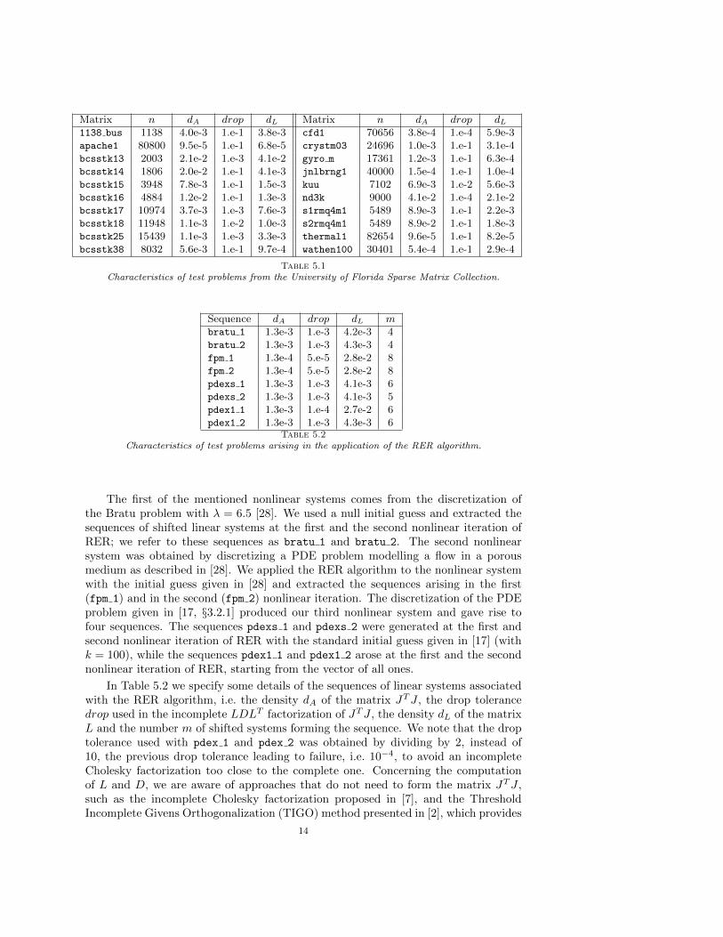
Matrix n dA drop dL Matrix n dA drop dL1138 bus 1138 4.0e-3 1.e-1 3.8e-3 cfd1 70656 3.8e-4 1.e-4 5.9e-3apache1 80800 9.5e-5 1.e-1 6.8e-5 crystm03 24696 1.0e-3 1.e-1 3.1e-4bcsstk13 2003 2.1e-2 1.e-3 4.1e-2 gyro m 17361 1.2e-3 1.e-1 6.3e-4bcsstk14 1806 2.0e-2 1.e-1 4.1e-3 jnlbrng1 40000 1.5e-4 1.e-1 1.0e-4bcsstk15 3948 7.8e-3 1.e-1 1.5e-3 kuu 7102 6.9e-3 1.e-2 5.6e-3bcsstk16 4884 1.2e-2 1.e-1 1.3e-3 nd3k 9000 4.1e-2 1.e-4 2.1e-2bcsstk17 10974 3.7e-3 1.e-3 7.6e-3 s1rmq4m1 5489 8.9e-3 1.e-1 2.2e-3bcsstk18 11948 1.1e-3 1.e-2 1.0e-3 s2rmq4m1 5489 8.9e-2 1.e-1 1.8e-3bcsstk25 15439 1.1e-3 1.e-3 3.3e-3 thermal1 82654 9.6e-5 1.e-1 8.2e-5bcsstk38 8032 5.6e-3 1.e-1 9.7e-4 wathen100 30401 5.4e-4 1.e-1 2.9e-4

Table 5.1

Characteristics of test problems from the University of Florida Sparse Matrix Collection.

Sequence dA drop dL mbratu 1 1.3e-3 1.e-3 4.2e-3 4bratu 2 1.3e-3 1.e-3 4.3e-3 4fpm 1 1.3e-4 5.e-5 2.8e-2 8fpm 2 1.3e-4 5.e-5 2.8e-2 8pdexs 1 1.3e-3 1.e-3 4.1e-3 6pdexs 2 1.3e-3 1.e-3 4.1e-3 5pdex1 1 1.3e-3 1.e-4 2.7e-2 6pdex1 2 1.3e-3 1.e-3 4.3e-3 6

Table 5.2

Characteristics of test problems arising in the application of the RER algorithm.

The first of the mentioned nonlinear systems comes from the discretization ofthe Bratu problem with λ = 6.5 [28]. We used a null initial guess and extracted thesequences of shifted linear systems at the first and the second nonlinear iteration ofRER; we refer to these sequences as bratu 1 and bratu 2. The second nonlinearsystem was obtained by discretizing a PDE problem modelling a flow in a porousmedium as described in [28]. We applied the RER algorithm to the nonlinear systemwith the initial guess given in [28] and extracted the sequences arising in the first(fpm 1) and in the second (fpm 2) nonlinear iteration. The discretization of the PDEproblem given in [17, §3.2.1] produced our third nonlinear system and gave rise tofour sequences. The sequences pdexs 1 and pdexs 2 were generated at the first andsecond nonlinear iteration of RER with the standard initial guess given in [17] (withk = 100), while the sequences pdex1 1 and pdex1 2 arose at the first and the secondnonlinear iteration of RER, starting from the vector of all ones.

In Table 5.2 we specify some details of the sequences of linear systems associatedwith the RER algorithm, i.e. the density dA of the matrix JTJ , the drop tolerancedrop used in the incomplete LDLT factorization of JTJ , the density dL of the matrixL and the number m of shifted systems forming the sequence. We note that the droptolerance used with pdex 1 and pdex 2 was obtained by dividing by 2, instead of10, the previous drop tolerance leading to failure, i.e. 10−4, to avoid an incompleteCholesky factorization too close to the complete one. Concerning the computationof L and D, we are aware of approaches that do not need to form the matrix JTJ ,such as the incomplete Cholesky factorization proposed in [7], and the ThresholdIncomplete Givens Orthogonalization (TIGO) method presented in [2], which provides

14

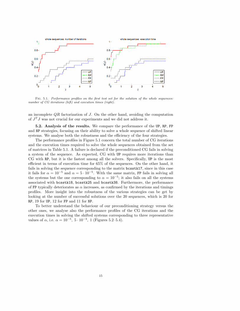
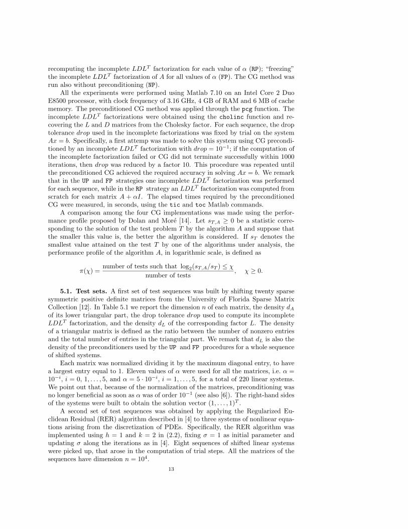
Fig. 5.1. Performance profiles on the first test set for the solution of the whole sequences:

number of CG iterations (left) and execution times (right).

an incomplete QR factorization of J . On the other hand, avoiding the computationof JTJ was not crucial for our experiments and we did not address it.

5.2. Analysis of the results. We compare the performance of the UP, RP, FPand NP strategies, focusing on their ability to solve a whole sequence of shifted linearsystems. We analyse both the robustness and the efficiency of the four strategies.

The performance profiles in Figure 5.1 concern the total number of CG iterationsand the execution times required to solve the whole sequences obtained from the setof matrices in Table 5.1. A failure is declared if the preconditioned CG fails in solvinga system of the sequence. As expected, CG with UP requires more iterations thanCG with RP, but it is the fastest among all the solvers. Specifically, UP is the mostefficient in terms of execution time for 65% of the sequences. On the other hand, itfails in solving the sequence corresponding to the matrix bcsstk17, since in this caseit fails for α = 10−5 and α = 5 · 10−5. With the same matrix, FP fails in solving allthe systems but the one corresponding to α = 10−5; it also fails on all the systemsassociated with bcsstk18, bcsstk25 and bcsstk38. Furthermore, the performanceof FP typically deteriorates as α increases, as confirmed by the iterations and timingsprofiles. More insight into the robustness of the various strategies can be get bylooking at the number of successful solutions over the 20 sequences, which is 20 forRP, 19 for UP, 12 for FP and 11 for NP.

To better understand the behaviour of our preconditioning strategy versus theother ones, we analyse also the performance profiles of the CG iterations and theexecution times in solving the shifted systems corresponding to three representativevalues of α, i.e. α = 10−5, 5 · 10−3, 1 (Figures 5.2–5.4).

15

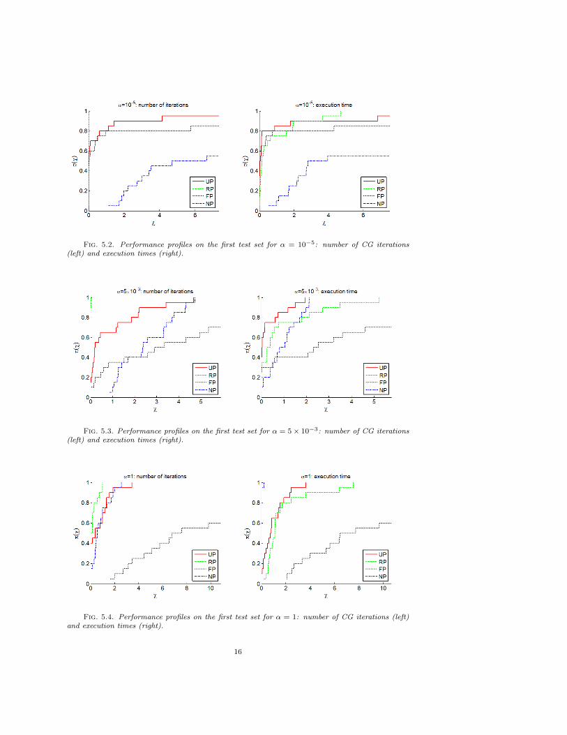
Fig. 5.2. Performance profiles on the first test set for α = 10−5: number of CG iterations

(left) and execution times (right).

Fig. 5.3. Performance profiles on the first test set for α = 5× 10−3: number of CG iterations

(left) and execution times (right).

Fig. 5.4. Performance profiles on the first test set for α = 1: number of CG iterations (left)

and execution times (right).

16

As expected, for each value of α, RP is the most efficient in terms of CG itera-tions, but not in terms of time. The performance of FP steadily deteriorates whileα increases and, for some tests, it already gives poor results with the small valueα = 10−5; more precisely, FP fails in solving 3, 6, 8 systems for α = 10−5, 5 · 10−3, 1,respectively. The NP strategy results in the slowest convergence rate and the largestexecution time until α becomes sufficiently large, i.e. when preconditioning is no longerneeded. Remarkably, the UP strategy is very effective in reducing the number of CGiterations and provides a good tradeoff between the cost of the linear solver and ofthe construction of the preconditioner. In particular, our strategy is the clear winnerin terms of execution time for α = 10−5 and α = 5 · 10−3, and shows a gain over RPand FP when α = 1.

In summary, we see that FP and NP work well for specific values of α, RP isexpensive in terms of time to solution, while the UP strategy shows a remarkablereliability and efficiency in solving sequences of shifted systems for a fairly broadrange of values of α.

We conclude the analysis of the first set of experiments reporting, in Tables 5.3and 5.4, the results for the sequences of systems built from the matrices nd3k ands1rmq4m1 (* denotes a CG failure). The test problem nd3k is representative of theconvergence history of CG with the various preconditioning techniques on several testproblems. In this case, NP fails for the first value of α, while it gains in iteration count(and time) as α increases; on the contrary, FP deteriorates for increasing values of α.The UP strategy generally behaves well for all values of α and is considerably fasterthan RP; in fact, the time for computing the preconditioner from scratch is relativelyhigh. In terms of execution time, the UP strategy outperforms the unpreconditionedCG as long as α ≤ 10−3. Concerning the sequence associated with s1rmq4m1, thetime for building the preconditioner from scratch for each matrix A+ αI is small, sothe RP strategy is fast. However, UP yields a number of CG iterations comparablewith that of RP and hence has a smaller execution time. More precisely, the relativetime saving of UP vs RP vary bewtween 9% and 46%. Finally, the execution times ofUP and RP compare favourably with the times of FP and NP for all values of α.

The results of our experiments on the second set of sequences are summarizedin Table 5.5, where the total number of CG iterations and the total execution timesfor solving all the systems of each sequence are reported. As for the first test set,we declare a failure (denoted by * in the table) when the preconditioned CG failsin solving at least one system of the sequence. We note that these sequences reallyneed a preconditioning strategy; in fact, the unpreconditioned CG fails in solving thefirst linear system of each sequence, corresponding to the smallest value of α. Forfive of the eight sequences, the UP strategy results to be the most efficient. Actually,for these sequences RP is the most effective in terms of CG iterations, but it requiresa significantly larger execution time than UP, because of the computation of the in-complete LDLT factorization for each value of α. The sequence pdex1 1 results hardto be solved, as only the RP strategy succeeds in its solution; our update strategyfails in solving the first linear system of the sequence. We observe also that on thefpm 1 and fpm 2 sequences the UP strategy requires a large number of CG iterationscompared to the RP one. Moreover, the small drop tolerance 5 · 10−5 that is neededfor computing an effective incomplete Cholesky preconditioner, produces a relativelydense factor L, hence the time required for applying the preconditioner, i.e. for solv-ing the related triangular systems at each CG iteration, is significant. Therefore, forthese two sequences, the considerable gain in terms of iterations obtained by the RP

17

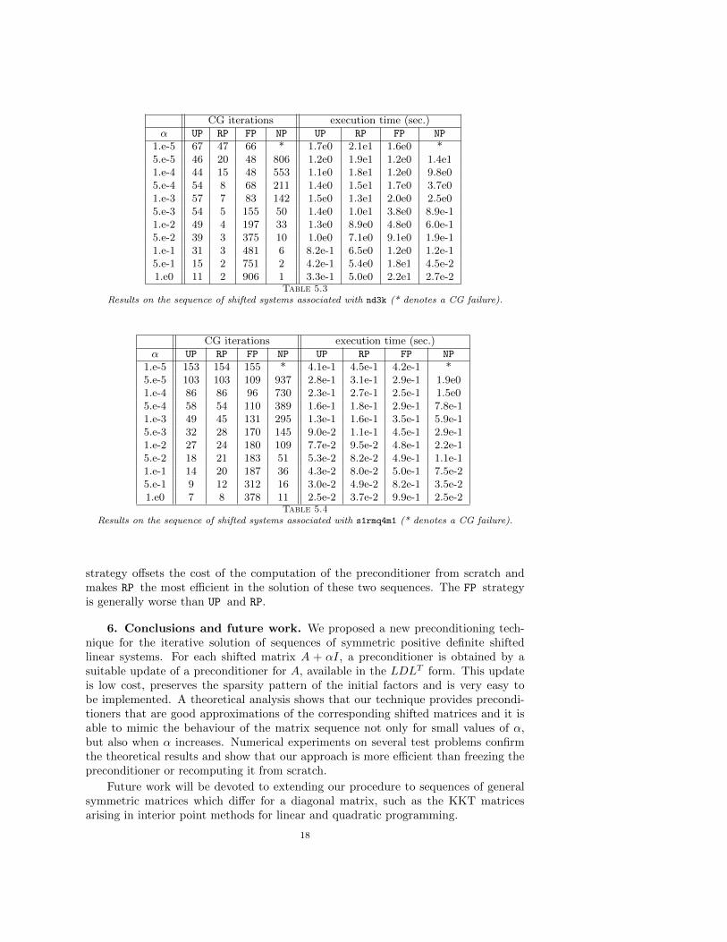
CG iterations execution time (sec.)α UP RP FP NP UP RP FP NP

1.e-5 67 47 66 * 1.7e0 2.1e1 1.6e0 *5.e-5 46 20 48 806 1.2e0 1.9e1 1.2e0 1.4e11.e-4 44 15 48 553 1.1e0 1.8e1 1.2e0 9.8e05.e-4 54 8 68 211 1.4e0 1.5e1 1.7e0 3.7e01.e-3 57 7 83 142 1.5e0 1.3e1 2.0e0 2.5e05.e-3 54 5 155 50 1.4e0 1.0e1 3.8e0 8.9e-11.e-2 49 4 197 33 1.3e0 8.9e0 4.8e0 6.0e-15.e-2 39 3 375 10 1.0e0 7.1e0 9.1e0 1.9e-11.e-1 31 3 481 6 8.2e-1 6.5e0 1.2e0 1.2e-15.e-1 15 2 751 2 4.2e-1 5.4e0 1.8e1 4.5e-21.e0 11 2 906 1 3.3e-1 5.0e0 2.2e1 2.7e-2

Table 5.3

Results on the sequence of shifted systems associated with nd3k (* denotes a CG failure).

CG iterations execution time (sec.)α UP RP FP NP UP RP FP NP

1.e-5 153 154 155 * 4.1e-1 4.5e-1 4.2e-1 *5.e-5 103 103 109 937 2.8e-1 3.1e-1 2.9e-1 1.9e01.e-4 86 86 96 730 2.3e-1 2.7e-1 2.5e-1 1.5e05.e-4 58 54 110 389 1.6e-1 1.8e-1 2.9e-1 7.8e-11.e-3 49 45 131 295 1.3e-1 1.6e-1 3.5e-1 5.9e-15.e-3 32 28 170 145 9.0e-2 1.1e-1 4.5e-1 2.9e-11.e-2 27 24 180 109 7.7e-2 9.5e-2 4.8e-1 2.2e-15.e-2 18 21 183 51 5.3e-2 8.2e-2 4.9e-1 1.1e-11.e-1 14 20 187 36 4.3e-2 8.0e-2 5.0e-1 7.5e-25.e-1 9 12 312 16 3.0e-2 4.9e-2 8.2e-1 3.5e-21.e0 7 8 378 11 2.5e-2 3.7e-2 9.9e-1 2.5e-2

Table 5.4

Results on the sequence of shifted systems associated with s1rmq4m1 (* denotes a CG failure).

strategy offsets the cost of the computation of the preconditioner from scratch andmakes RP the most efficient in the solution of these two sequences. The FP strategyis generally worse than UP and RP.

6. Conclusions and future work. We proposed a new preconditioning tech-nique for the iterative solution of sequences of symmetric positive definite shiftedlinear systems. For each shifted matrix A + αI, a preconditioner is obtained by asuitable update of a preconditioner for A, available in the LDLT form. This updateis low cost, preserves the sparsity pattern of the initial factors and is very easy tobe implemented. A theoretical analysis shows that our technique provides precondi-tioners that are good approximations of the corresponding shifted matrices and it isable to mimic the behaviour of the matrix sequence not only for small values of α,but also when α increases. Numerical experiments on several test problems confirmthe theoretical results and show that our approach is more efficient than freezing thepreconditioner or recomputing it from scratch.

Future work will be devoted to extending our procedure to sequences of generalsymmetric matrices which differ for a diagonal matrix, such as the KKT matricesarising in interior point methods for linear and quadratic programming.

18

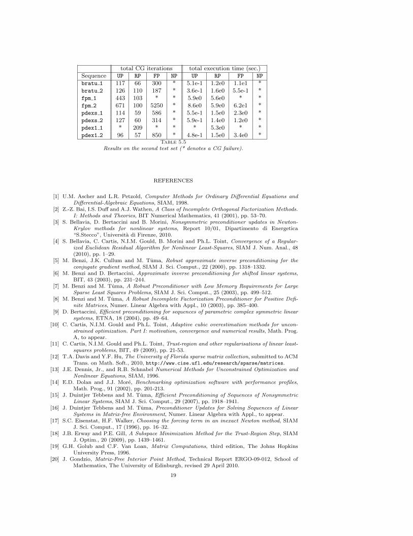
total CG iterations total execution time (sec.)Sequence UP RP FP NP UP RP FP NPbratu 1 117 66 300 * 5.1e-1 1.2e0 1.1e1 *bratu 2 126 110 187 * 3.6e-1 1.6e0 5.5e-1 *fpm 1 443 103 * * 5.9e0 5.6e0 * *fpm 2 671 100 5250 * 8.6e0 5.9e0 6.2e1 *pdexs 1 114 59 586 * 5.5e-1 1.5e0 2.3e0 *pdexs 2 127 60 314 * 5.9e-1 1.4e0 1.2e0 *pdex1 1 * 209 * * * 5.3e0 * *pdex1 2 96 57 850 * 4.8e-1 1.5e0 3.4e0 *

Table 5.5

Results on the second test set (* denotes a CG failure).

REFERENCES

[1] U.M. Ascher and L.R. Petzold, Computer Methods for Ordinary Differential Equations and

Differential-Algebraic Equations, SIAM, 1998.[2] Z.-Z. Bai, I.S. Duff and A.J. Wathen, A Class of Incomplete Orthogonal Factorization Methods.

I: Methods and Theories, BIT Numerical Mathematics, 41 (2001), pp. 53–70.[3] S. Bellavia, D. Bertaccini and B. Morini, Nonsymmetric preconditioner updates in Newton-

Krylov methods for nonlinear systems, Report 10/01, Dipartimento di Energetica“S.Stecco”, Universita di Firenze, 2010.

[4] S. Bellavia, C. Cartis, N.I.M. Gould, B. Morini and Ph.L. Toint, Convergence of a Regular-

ized Euclidean Residual Algorithm for Nonlinear Least-Squares, SIAM J. Num. Anal., 48(2010), pp. 1–29.

[5] M. Benzi, J.K. Cullum and M. Tuma, Robust approximate inverse preconditioning for the

conjugate gradient method, SIAM J. Sci. Comput., 22 (2000), pp. 1318–1332.[6] M. Benzi and D. Bertaccini, Approximate inverse preconditioning for shifted linear systems,

BIT, 43 (2003), pp. 231–244.[7] M. Benzi and M. Tuma, A Robust Preconditioner with Low Memory Requirements for Large

Sparse Least Squares Problems, SIAM J. Sci. Comput., 25 (2003), pp. 499–512.[8] M. Benzi and M. Tuma, A Robust Incomplete Factorization Preconditioner for Positive Defi-

nite Matrices, Numer. Linear Algebra with Appl., 10 (2003), pp. 385–400.[9] D. Bertaccini, Efficient preconditioning for sequences of parametric complex symmetric linear

systems, ETNA, 18 (2004), pp. 49–64.[10] C. Cartis, N.I.M. Gould and Ph.L. Toint, Adaptive cubic overestimation methods for uncon-

strained optimization. Part I: motivation, convergence and numerical results, Math. Prog.A, to appear.

[11] C. Cartis, N.I.M. Gould and Ph.L. Toint, Trust-region and other regularisations of linear least-

squares problems, BIT, 49 (2009), pp. 21-53.[12] T.A. Davis and Y.F. Hu, The University of Florida sparse matrix collection, submitted to ACM

Trans. on Math. Soft., 2010, http://www.cise.ufl.edu/research/sparse/matrices.[13] J.E. Dennis, Jr., and R.B. Schnabel Numerical Methods for Unconstrained Optimization and

Nonlinear Equations, SIAM, 1996.[14] E.D. Dolan and J.J. More, Benchmarking optimization software with performance profiles,

Math. Prog., 91 (2002), pp. 201-213.[15] J. Duintjer Tebbens and M. Tuma, Efficient Preconditioning of Sequences of Nonsymmetric

Linear Systems, SIAM J. Sci. Comput., 29 (2007), pp. 1918–1941.[16] J. Duintjer Tebbens and M. Tuma, Preconditioner Updates for Solving Sequences of Linear

Systems in Matrix-free Environment, Numer. Linear Algebra with Appl., to appear.[17] S.C. Eisenstat, H.F. Walker, Choosing the forcing term in an inexact Newton method, SIAM

J. Sci. Comput., 17 (1996), pp. 16–32.[18] J.B. Erway and P.E. Gill, A Subspace Minimization Method for the Trust-Region Step, SIAM

J. Optim., 20 (2009), pp. 1439–1461.[19] G.H. Golub and C.F. Van Loan, Matrix Computations, third edition, The Johns Hopkins

University Press, 1996.[20] J. Gondzio, Matrix-Free Interior Point Method, Technical Report ERGO-09-012, School of

Mathematics, The University of Edinburgh, revised 29 April 2010.

19

[21] N.I.M. Gould, D.P. Robinson and H.S. Thorne, On solving trust-region and other regularised

subproblems in optimization, Math. Program. Comput., 2 (2010), pp. 21–57.[22] R.A. Horn and C.R. Johnson, Topics in Matrix Analysis, Cambridge University Press, 1991.[23] G. Meurant, On the incomplete Cholesky decomposition of a class of perturbed matrices, SIAM

J. Sci. Comput., 23 (2001), pp. 419–429.[24] J. J. More and D.C. Sorensen, Computing a trust-region step, SIAM J. Sci. Stat. Comput., 4

(1983), pp. 553–572.[25] Y. Nesterov, Modified Gauss-Newton scheme with worst-case guarantees for global performance,

Optim. Methods Softw., 22 (2007), pp.469–483.[26] J. Nocedal and S.J. Wright, Numerical Optimization, Springer Series in Operation Research,

Springer-Verlag, 1999.[27] C.C. Paige and M.A. Saunders, LSQR: An algorithm for sparse linear equations and sparse

least squares, ACM Trans. Math. Soft. 8 (1982), pp. 43–71.[28] M. Pernice and H.F. Walker, NITSOL: a new iterative solver for nonlinear systems, SIAM

J. Sci. Comput., 19 (1998), pp. 302–318.

20