Veronica Felli Dipartimento di Matematica ed Applicazioni ...felli/talks/sem_dottorato_2011.pdf ·...
81
Elliptic and parabolic equations with singular potentials Veronica Felli Dipartimento di Matematica ed Applicazioni University of Milano–Bicocca [email protected] – p. 1
Transcript of Veronica Felli Dipartimento di Matematica ed Applicazioni ...felli/talks/sem_dottorato_2011.pdf ·...

Elliptic and parabolic equations with singular potentials
Veronica Felli
Dipartimento di Matematica ed Applicazioni
University of Milano–Bicocca
– p. 1

Problem:describe the behavior at the singularity of solutions to equationsassociated to Schrodinger operators with singular homogeneouspotentials (with the same order of homogeneity of the operator)
La := −∆− a(x/|x|)|x|2 , x ∈ R
N , a : SN−1 → R, N > 3
– p. 2

Problem:describe the behavior at the singularity of solutions to equationsassociated to Schrodinger operators with singular homogeneouspotentials (with the same order of homogeneity of the operator)
La := −∆− a(x/|x|)|x|2 , x ∈ R
N , a : SN−1 → R, N > 3
Examples
Dipole-potential : −~2
2m∆+ e
x ·D
|x|3 a(θ) = λθ ·D
Quantummany-body :
M∑
j=1
−∆j
2mj+
M∑
j,m=1j<m
λjλm
|xj − xm|2 a(θ) =∑ λjλm
|θj − θm|2
xj ∈ Rd, N =Md, θj = xj/|x|, x = (x1, . . . , xM ) ∈ RN
– p. 2

Problem: describe the asymptotic behavior at the singularity of solutionsto equations associated to Schrodinger operators with singularhomogeneous electromagnetic potentials
LA,a :=
(
−i∇+A(x|x|
)
|x|
)2
−a(x|x|
)
|x|2 , A ∈ C1(SN−1,RN )
– p. 3

Problem: describe the asymptotic behavior at the singularity of solutionsto equations associated to Schrodinger operators with singularhomogeneous electromagnetic potentials
LA,a :=
(
−i∇+A(x|x|
)
|x|
)2
−a(x|x|
)
|x|2 , A ∈ C1(SN−1,RN )
Example: Aharonov-Bohm magnetic potentials associated to thinsolenoids; if the radius of the solenoid tends to zero while theflux through it remains constant, then the particle is subject to aδ-type magnetic field, which is called Aharonov-Bohm field.
A( x|x|
)
|x|= α
(
−x2
|x|2,x1
|x|2
)
, x = (x1, x2) ∈ R2
A(θ1, θ2) = α(−θ2, θ1), (θ1, θ2) ∈ S1,
with α = circulation around the solenoid.
– p. 3

Motivation
• regularity theory for elliptic operators with singularities of Fuchsian type[Mazzeo, Comm. PDE’s(1991)], [Pinchover , Ann. IHP(1994)]
– p. 4

Motivation
• regularity theory for elliptic operators with singularities of Fuchsian type[Mazzeo, Comm. PDE’s(1991)], [Pinchover , Ann. IHP(1994)]
• asymptotics at singular sets is expected to provide informations about the“critical dimension” for existence of solutions to problems with criticalgrowth (Brezis-Nirenberg type results)[Jannelli , J. Diff. Eq.(1999)], [Ferrero-Gazzola , J. Diff. Eq.(2001)]
• the asymptotic analysis is also a tool for the construction of solutions toSchrodinger equations with singular potentials[F.-Terracini , Comm. PDE’s(2006)][Abdellaoui-F.-Peral , Calc. Var. PDE’s(2009)]
• the knowledge of exact asymptotics of solutions at the poles is crucial inthe study of spectral properties (essential self-adjointness)[F.-Marchini-Terracini , J. Funct. Anal.(2007)][F.-Marchini-Terracini , Indiana Univ. Math. J.(2009)]
– p. 4

References
[F.-Schneider, Adv. Nonl. Studies (2003)] : Holder continuity results fordegenerate elliptic equations with singular weights; include asymptotics of
solutions near the pole for potentials λ|x|2 (a(θ) constant).
– p. 5

References
[F.-Schneider, Adv. Nonl. Studies (2003)] : Holder continuity results fordegenerate elliptic equations with singular weights; include asymptotics of
solutions near the pole for potentials λ|x|2 (a(θ) constant).
[F.-Marchini-Terracini, Discrete Contin. Dynam. Systems (20 08)]: exactasymptotics of solutions near the pole for anisotropic inverse-square singular
potentialsa(x/|x|)
|x|2 (a(θ) bounded), through separation of variables and
comparison methods.
[F.-Ferrero-Terracini, J. Europ. Math. Soc. (2011)] : singular homogeneouselectromagnetic potentials of Aharonov-Bohm type, by an Almgren typemonotonicity formula and blow-up methods.
[F.-Ferrero-Terracini, Preprint 2010] : behavior at collisions of solutions toSchrodinger equations with many-particle and cylindrical potentials by anonlinear Almgren type formula and blow-up.
– p. 5

Outline of the talk
1. Elliptic monotonicity formula
– p. 6

Outline of the talk
1. Elliptic monotonicity formula
2. Asymptotics at singularities (elliptic case)
– p. 6

Outline of the talk
1. Elliptic monotonicity formula
2. Asymptotics at singularities (elliptic case)
3. Parabolic monotonicity formula
– p. 6

Outline of the talk
1. Elliptic monotonicity formula
2. Asymptotics at singularities (elliptic case)
3. Parabolic monotonicity formula
4. Asymptotics at singularities (parabolic case)
– p. 6

1. Elliptic monotonicity formula
Studying regularity of area-minimizing surfaces of codimension> 1, in 1979 F. Almgren introduced the frequency function
N (r) =r2−N
∫
Br|∇u|2 dx
r1−N∫
∂Bru2
and observed that, if u is harmonic, then N ր in r .
– p. 7

1. Elliptic monotonicity formula
Studying regularity of area-minimizing surfaces of codimension> 1, in 1979 F. Almgren introduced the frequency function
N (r) =r2−N
∫
Br|∇u|2 dx
r1−N∫
∂Bru2
and observed that, if u is harmonic, then N ր in r .
Proof:
N ′(r) =
2r
[(∫
∂Br
∣∣∂u∂ν
∣∣2dS)(∫
∂Br|u|2dS
)
−(∫
∂Bru∂u∂ν dS
)2]
(∫
∂Br|u|2dS
)2
Schwarz’s>
inequality0
– p. 7

Why frequency?
If N ≡ γ is constant, then N ′(r) = 0, i.e.
(∫
∂Br
∣∣∣∣
∂u
∂ν
∣∣∣∣
2
dS
)
·(∫
∂Br
u2dS
)
−(∫
∂Br
u∂u
∂νdS
)2
= 0
=⇒ u and ∂u∂ν are parallel as vectors in L2(∂Br), i.e. ∃ η(r) s. t.
∂u
∂ν(r, θ) = η(r)u(r, θ), i.e.
d
drlog |u(r, θ)| = η(r).
– p. 8

Why frequency?
If N ≡ γ is constant, then N ′(r) = 0, i.e.
(∫
∂Br
∣∣∣∣
∂u
∂ν
∣∣∣∣
2
dS
)
·(∫
∂Br
u2dS
)
−(∫
∂Br
u∂u
∂νdS
)2
= 0
=⇒ u and ∂u∂ν are parallel as vectors in L2(∂Br), i.e. ∃ η(r) s. t.
∂u
∂ν(r, θ) = η(r)u(r, θ), i.e.
d
drlog |u(r, θ)| = η(r).
After integration we obtain
u(r, θ)= e∫ r
1η(s)dsu(1, θ) = ϕ(r)ψ(θ).
– p. 8

Why frequency? u(r, θ) = ϕ(r)ψ(θ) and ∆u = 0
⇓(ϕ′′(r) + N−1
r ϕ′(r))ψ(θ) + r−2ϕ(r)∆SN−1ψ(θ) = 0.
– p. 9

Why frequency? u(r, θ) = ϕ(r)ψ(θ) and ∆u = 0
⇓(ϕ′′(r) + N−1
r ϕ′(r))ψ(θ) + r−2ϕ(r)∆SN−1ψ(θ) = 0.
ψ is a spherical harmonic ⇒ ∃ k ∈ N s.t. −∆SN−1ψ = k(N − 2 + k)ψ
−ϕ′′(r)− N−1r ϕ(r) + r−2k(N − 2 + k)ϕ(r) = 0.
– p. 9

Why frequency? u(r, θ) = ϕ(r)ψ(θ) and ∆u = 0
⇓(ϕ′′(r) + N−1
r ϕ′(r))ψ(θ) + r−2ϕ(r)∆SN−1ψ(θ) = 0.
ψ is a spherical harmonic ⇒ ∃ k ∈ N s.t. −∆SN−1ψ = k(N − 2 + k)ψ
−ϕ′′(r)− N−1r ϕ(r) + r−2k(N − 2 + k)ϕ(r) = 0.
ϕ(r) = c1rσ+
+ c2rσ−
with σ± = −N−22 ± 1
2 (2k +N − 2)
σ+ = k, σ− = −(N − 2)− k
|x|σ−
ψ( x|x| ) /∈ H1(B1) ; c2 = 0, ϕ(1) = 1 ; c1 = 1
⇓u(r, θ) = rkψ(θ)
From N (r) ≡ γ, we deduce that γ = k.
– p. 9

Applications to elliptic PDE’s
The Almgren monotonicity formula was used in• [Garofalo-Lin, Indiana Univ. Math. J. (1986)] :
generalization to variable coefficient elliptic operators indivergence form (unique continuation)
• [Athanasopoulos-Caffarelli-Salsa, Amer. J. Math. (2008)] :regularity of the free boundary in obstacle problems.
• [Caffarelli-Lin, J. AMS (2008)] regularity of free boundary of thelimit components of singularly perturbed elliptic systems.
– p. 10

Perturbed monotonicity
Example (Garofalo-Lin). Let u ∈ H1loc(B1) be a weak solution to
−∆u(x) + V (x)u = 0 in B1,
with V ∈ L∞loc(B1). Define
D(r) = 1rN−2
∫
Br
[∣∣∇u
∣∣2+ V |u|2
]
dx
H(r) = 1rN−1
∫
∂Br
|u|2 dS
Almgren type function
N (r) =D(r)
H(r)
– p. 11

Perturbed monotonicity
Example (Garofalo-Lin). Let u ∈ H1loc(B1) be a weak solution to
−∆u(x) + V (x)u = 0 in B1,
with V ∈ L∞loc(B1). Define
D(r) = 1rN−2
∫
Br
[∣∣∇u
∣∣2+ V |u|2
]
dx
H(r) = 1rN−1
∫
∂Br
|u|2 dS
Almgren type function
N (r) =D(r)
H(r)
N ′(r) =
2r
[(∫
∂Br
∣∣∂u∂ν
∣∣2dS)(∫
∂Br|u|2dS
)
−(∫
∂Bru∂u
∂ν dS)2]
(∫
∂Br|u|2dS
)2 +R(r)
6
0– p. 11

Perturbed monotonicity
R(r) = −2[ ∫
BrV u (x · ∇u) dx+ N−2
2
∫
BrV u2 dx− r
2
∫
∂BrV u2 dS
]
∫
∂Br|u|2dS
– p. 12

Perturbed monotonicity
R(r) = −2[ ∫
BrV u (x · ∇u) dx+ N−2
2
∫
BrV u2 dx− r
2
∫
∂BrV u2 dS
]
∫
∂Br|u|2dS
|R(r)| 6 C1 r(N (r) + C2)
– p. 12

Perturbed monotonicity
R(r) = −2[ ∫
BrV u (x · ∇u) dx+ N−2
2
∫
BrV u2 dx− r
2
∫
∂BrV u2 dS
]
∫
∂Br|u|2dS
|R(r)| 6 C1 r(N (r) + C2)
N ′(r) > −C1r(N (r) + C2) i.e.d
drlog(N (r) + C2) > −C1r
– p. 12

Perturbed monotonicity
R(r) = −2[ ∫
BrV u (x · ∇u) dx+ N−2
2
∫
BrV u2 dx− r
2
∫
∂BrV u2 dS
]
∫
∂Br|u|2dS
|R(r)| 6 C1 r(N (r) + C2)
N ′(r) > −C1r(N (r) + C2) i.e.d
drlog(N (r) + C2) > −C1r
integrate between r and r N (r) + C2 6 (N (r) + C2)eC1
2r2 6 const
In particular, N is bounded.
– p. 12

Perturbed monotonicity
H(r) =1
rN−1
∫
∂Br
|u|2 dS =⇒ H ′(r) =2
rN−1
∫
∂Br
u∂u
∂νdS
– p. 13

Perturbed monotonicity
H(r) =1
rN−1
∫
∂Br
|u|2 dS =⇒ H ′(r) =2
rN−1
∫
∂Br
u∂u
∂νdS
Test −∆u(x) + V (x)u = 0 with u =⇒∫
Br
[∣∣∇u
∣∣2 + V |u|2
]
dx =
∫
∂Br
u∂u
∂νdS
– p. 13

Perturbed monotonicity
H(r) =1
rN−1
∫
∂Br
|u|2 dS =⇒ H ′(r) =2
rN−1
∫
∂Br
u∂u
∂νdS
Test −∆u(x) + V (x)u = 0 with u =⇒
rN−2D(r) =
∫
Br
[∣∣∇u
∣∣2+V |u|2
]
dx =
∫
∂Br
u∂u
∂νdS =
rN−1
2H ′(r)
– p. 13

Perturbed monotonicity
H(r) =1
rN−1
∫
∂Br
|u|2 dS =⇒ H ′(r) =2
rN−1
∫
∂Br
u∂u
∂νdS
Test −∆u(x) + V (x)u = 0 with u =⇒
rN−2D(r) =
∫
Br
[∣∣∇u
∣∣2+V |u|2
]
dx =
∫
∂Br
u∂u
∂νdS =
rN−1
2H ′(r)
Hence H′(r)H(r) = 2
rN (r) 6 constr , i.e. d
dr logH(r) 6 Cr .
Integrating between R and 2R
logH(2R)
H(R)6 C log 2 i.e.
∫
∂B2R
u2 dS 6 const
∫
∂BR
u2 dS
– p. 13

Doubling and unique continuation
Doubling condition
∫
B2R
u2 dx 6 Cdoub
∫
BR
u2 dx
with Cdoub independent of R
– p. 14

Doubling and unique continuation
Doubling condition
∫
B2R
u2 dx 6 Cdoub
∫
BR
u2 dx
with Cdoub independent of R
⇓
Strong unique continuation property
If u vanishes of infinite order at 0, i.e.∫
BR
u2 dx = O(Rm) as R→ 0 ∀m ∈ N,
then u ≡ 0 in B1.
– p. 14

Doubling and unique continuation
Proof. Let m0 s.t.Cdoub
2m0
< 1.
Hence∫
B1
u2dx 6 Cdoub
∫
B1/2
u2dx 6 · · · 6
6 Cndoub
∫
B2−n
u2dx 6n large
CndoubC(m0)(2−n)m0
= C(m0)(Cdoub
2m0
)n n→∞−→ 0
Hence∫
B1u2dx = 0, i.e. u ≡ 0 in B1.
– p. 15
2. Asymptotics at singularities (elliptic case)
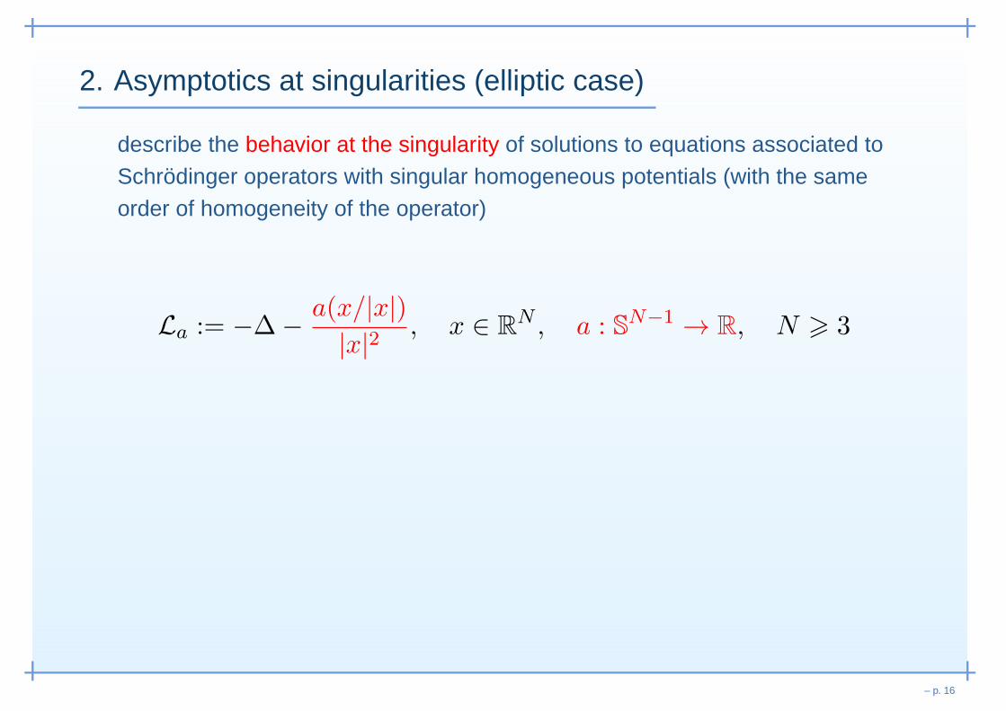
describe the behavior at the singularity of solutions to equations associated toSchrodinger operators with singular homogeneous potentials (with the sameorder of homogeneity of the operator)
La := −∆− a(x/|x|)|x|2 , x ∈ R
N , a : SN−1 → R, N > 3
– p. 16

Hardy type inequalities
Λ(a) := supu∈D1,2\0
∫
RN
|x|−2a(x/|x|)u2(x) dx∫
RN
|∇u(x)|2 dx
• Classical Hardy’s inequality: Λ(1) =(
2N−2
)2.
• If a ∈ L∞(SN−1), classical Hardy’s inequality ⇒ Λ(a) < +∞.
• For many body potentials a(x/|x|)|x|2 =
∑Mj<m
λjλm
|xj−xm|2 ,
Maz’ja and Badiale-Tarantello inequalities ⇒ Λ(a) < +∞.
– p. 17

Hardy type inequalities
Λ(a) := supu∈D1,2\0
∫
RN
|x|−2a(x/|x|)u2(x) dx∫
RN
|∇u(x)|2 dx
• Classical Hardy’s inequality: Λ(1) =(
2N−2
)2.
• If a ∈ L∞(SN−1), classical Hardy’s inequality ⇒ Λ(a) < +∞.
• For many body potentials a(x/|x|)|x|2 =
∑Mj<m
λjλm
|xj−xm|2 ,
Maz’ja and Badiale-Tarantello inequalities ⇒ Λ(a) < +∞.
The quadratic form associated to
La = −∆− a(x/|x|)|x|2 is positive definite in D1,2 ⇐⇒ Λ(a) < 1
– p. 17

Perturbations of La
linear /semilinear perturbations of La: Lau = h(x)u(x) + f(x,u(x))
– p. 18

Perturbations of La
linear /semilinear perturbations of La: Lau = h(x)u(x) + f(x,u(x))
(H) h “negligible” with respect toa(x/|x|)
|x|2 at singularity:
limr→0+
η0(r) = 0,η0(r)
r∈ L1,
1
r
∫ r
0
η0(s)
sds ∈ L1,
η1(r)
r∈ L1,
1
r
∫ r
0
η1(s)
sds ∈ L1,
where η0(r) = supu∈H1(Br)
u 6≡0
∫
Br|h(x)|u2dx
∫
Br(|∇u|2 −
a(x/|x|)
|x|2u2)dx+ N−2
2r
∫
∂Bru2dS
,
η1(r) = supu∈H1(Br)
u 6≡0
∫
Br|∇h · x|u2dx
∫
Br(|∇u|2 −
a(x/|x|)
|x|2u2)dx+ N−2
2r
∫
∂Bru2dS
– p. 18

Perturbations of La
linear /semilinear perturbations of La: Lau = h(x)u(x) + f(x,u(x))
(H) h “negligible” with respect toa(x/|x|)
|x|2 at singularity:
limr→0+
η0(r) = 0,η0(r)
r∈ L1,
1
r
∫ r
0
η0(s)
sds ∈ L1,
η1(r)
r∈ L1,
1
r
∫ r
0
η1(s)
sds ∈ L1,
Examples: • h, (x · ∇h) ∈ Ls for some s > N/2
• a ∈ L∞(SN−1) ; h(x) = O(|x|−2+ε)
•a(x/|x|)
|x|2=
∑
j,m
λjλm
|xj − xm|2; |h(x)|+ |∇h · x| = O
(
∑
|xj − xm|−2+ε)
(F) f at most critical: |f(x, s)s|+ |f ′s(x, s)s2|+ |∇xF (x, s) · x|6Cf (|s|
2 + |s|2∗
)
where F (x, s) =∫ s0 f(x, t) dt, 2∗ = 2N
N−2.
– p. 18

The angular operatorWe aim to describe the rate and the shape ofthe singularity of solutions, by relating them to theeigenvalues and the eigenfunctions of a
Schrodinger operator on SN−1 corresponding to the angular part of La:
La := −∆SN−1 − a
– p. 19

The angular operatorWe aim to describe the rate and the shape ofthe singularity of solutions, by relating them to theeigenvalues and the eigenfunctions of a
Schrodinger operator on SN−1 corresponding to the angular part of La:
La := −∆SN−1 − a
If Λ(a) < 1, La admits a diverging sequence of real eigenvalues
µ1(a) < µ2(a) 6 · · · 6 µk(a) 6 · · ·
Positivity of the quadratic formassociated to La
Λ(a) < 1
⇐⇒ µ1(a) > −(N−22
)2(PD)
– p. 19

The Almgren type frequency function
In an open bounded Ω ∋ 0, let u be a H1(Ω)-weak solution to
Lau = h(x)u(x) + f(x, u(x))
For small r > 0 define
D(r) =1
rN−2
∫
Br
(
|∇u(x)|2 −a( x
|x| )
|x|2 u2(x)− h(x)u2(x)− f(x, u(x))u(x)
)
dx,
H(r) =1
rN−1
∫
∂Br
|u|2 dS.
– p. 20

The Almgren type frequency function
In an open bounded Ω ∋ 0, let u be a H1(Ω)-weak solution to
Lau = h(x)u(x) + f(x, u(x))
For small r > 0 define
D(r) =1
rN−2
∫
Br
(
|∇u(x)|2 −a( x
|x| )
|x|2 u2(x)− h(x)u2(x)− f(x, u(x))u(x)
)
dx,
H(r) =1
rN−1
∫
∂Br
|u|2 dS.
If (PD) holds and u 6≡ 0,⇒ H(r) > 0 for small r > 0
;
Almgren type frequency function
N (r) = Nu,h,f (r) =D(r)
H(r)
is well defined in a suitably small interval (0, r0).
– p. 20

“Perturbed monotonicity” N ′ is an integrable perturbation of anonnegative function: enough to provethe existence of limr→0+ N (r)
– p. 21

“Perturbed monotonicity” N ′ is an integrable perturbation of anonnegative function: enough to provethe existence of limr→0+ N (r)
N ∈W 1,1loc (0, r0) and, in a distributional sense and for a.e. r ∈ (0, r0),
N ′(r) =
2r
[(∫
∂Br
∣∣∂u∂ν
∣∣2dS)(∫
∂Br|u|2dS
)
−(∫
∂Bru∂u
∂ν dS)2]
(∫
∂Br|u|2dS
)2 + (Rh +R1f +R2
f )(r)
Rh(r) = −
∫
Br(2h(x) +∇h(x) · x)|u|2 dx
∫
∂Br|u|2 dS
, R1f (r) =
r∫
∂Br
(
2F (x, u)− f(x, u)u)
dS∫
∂Br|u|2 dS
R2f (r) =
∫
Br
(
(N − 2)f(x, u)u− 2NF (x, u)− 2∇xF (x, u) · x)
dx∫
∂Br|u|2 dS
.
– p. 21

“Perturbed monotonicity” N ′ is an integrable perturbation of anonnegative function: enough to provethe existence of limr→0+ N (r)
N ∈W 1,1loc (0, r0) and, in a distributional sense and for a.e. r ∈ (0, r0),
N ′(r) =
2r
[(∫
∂Br
∣∣∂u∂ν
∣∣2dS)(∫
∂Br|u|2dS
)
−(∫
∂Bru∂u
∂ν dS)2]
(∫
∂Br|u|2dS
)2 + (Rh +R1f +R2
f )(r)
︸ ︷︷ ︸
Schwarz’s inequality6
0
Rh(r) = −
∫
Br(2h(x) +∇h(x) · x)|u|2 dx
∫
∂Br|u|2 dS
, R1f (r) =
r∫
∂Br
(
2F (x, u)− f(x, u)u)
dS∫
∂Br|u|2 dS
R2f (r) =
∫
Br
(
(N − 2)f(x, u)u− 2NF (x, u)− 2∇xF (x, u) · x)
dx∫
∂Br|u|2 dS
.
︸ ︷︷ ︸
integrable
– p. 21

“Perturbed monotonicity” N ′ is an integrable perturbation of anonnegative function: enough to provethe existence of limr→0+ N (r)
N ∈W 1,1loc (0, r0) and, in a distributional sense and for a.e. r ∈ (0, r0),
N ′(r) =
2r
[(∫
∂Br
∣∣∂u∂ν
∣∣2dS)(∫
∂Br|u|2dS
)
−(∫
∂Bru∂u
∂ν dS)2]
(∫
∂Br|u|2dS
)2 + (Rh +R1f +R2
f )(r)
︸ ︷︷ ︸
Schwarz’s inequality6
0
N ′ = nonnegative function + L1-function on (0, r) =⇒
N (r) = N (r)−∫ r
rN ′(s) ds
admits a limit γ as r → 0+
which is necessarily finite
︸ ︷︷ ︸
integrable
– p. 22

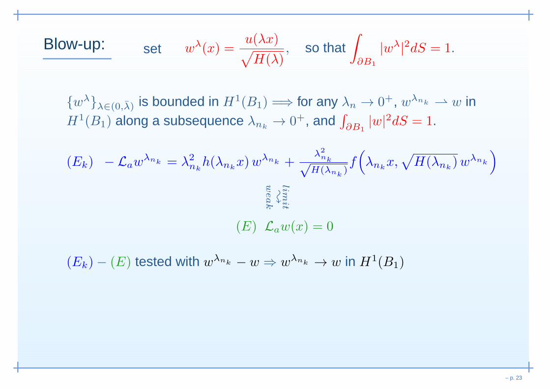
Blow-up: set wλ(x) =u(λx)√
H(λ), so that
∫
∂B1
|wλ|2dS = 1.
wλλ∈(0,λ) is bounded in H1(B1) =⇒ for any λn → 0+, wλnk w inH1(B1) along a subsequence λnk
→ 0+, and∫
∂B1|w|2dS = 1.
– p. 23
Blow-up: set wλ(x) =u(λx)√
H(λ), so that
∫
∂B1
|wλ|2dS = 1.
wλλ∈(0,λ) is bounded in H1(B1) =⇒ for any λn → 0+, wλnk w inH1(B1) along a subsequence λnk
→ 0+, and∫
∂B1|w|2dS = 1.
(Ek) − Lawλnk = λ2nk
h(λnkx)wλnk +
λ2nk√
H(λnk)f(
λnkx,√
H(λnk)wλnk
)
limit
;
weak
(E) Law(x) = 0
(Ek)− (E) tested with wλnk − w ⇒ wλnk → w in H1(B1)
– p. 23

Blow-up: set wλ(x) =u(λx)√
H(λ), so that
∫
∂B1
|wλ|2dS = 1.
wλλ∈(0,λ) is bounded in H1(B1) =⇒ for any λn → 0+, wλnk w inH1(B1) along a subsequence λnk
→ 0+, and∫
∂B1|w|2dS = 1.
(Ek) − Lawλnk = λ2nk
h(λnkx)wλnk +
λ2nk√
H(λnk)f(
λnkx,√
H(λnk)wλnk
)
limit
;
weak
(E) Law(x) = 0
(Ek)− (E) tested with wλnk − w ⇒ wλnk → w in H1(B1)
If Nk(r) the Almgren frequency function associated to (Ek) andNw(r) is the Almgren frequency function associated to (E), then
limk→∞
Nk(r) = Nw(r) for all r ∈ (0, 1).
– p. 23

Blow-up: By scaling Nk(r) = N (λnkr)
⇓Nw(r) = lim
k→∞N (λnk
r)= γ ∀r ∈ (0, 1)
– p. 24

Blow-up: By scaling Nk(r) = N (λnkr)
⇓Nw(r) = lim
k→∞N (λnk
r)= γ ∀r ∈ (0, 1)
Then Nw is constant in (0, 1) and hence N ′w(r) = 0 for any r ∈ (0, 1)
⇓(∫
∂Br
∣∣∣∣
∂w
∂ν
∣∣∣∣
2
dS
)
·(∫
∂Br
|w|2dS)
−(∫
∂Br
w∂w
∂νdS
)2
= 0
Therefore w and ∂w∂ν are parallel as vectors in L2(∂Br), i.e. ∃ a real
valued function η = η(r) such that ∂w∂ν (r, θ) = η(r)w(r, θ) for r ∈ (0, 1).
After integration we obtain
w(r, θ)= e∫ r1η(s)dsw(1, θ) = ϕ(r)ψ(θ).
– p. 24

Blow-up: w(r, θ) = ϕ(r)ψ(θ)
Rewriting equation (E) Law(x) = 0 in polar coordinates we obtain(−ϕ′′(r)− N−1
r ϕ′(r))ψ(θ) + r−2ϕ(r)Laψ(θ) = 0.
– p. 25

Blow-up: w(r, θ) = ϕ(r)ψ(θ)
Rewriting equation (E) Law(x) = 0 in polar coordinates we obtain(−ϕ′′(r)− N−1
r ϕ′(r))ψ(θ) + r−2ϕ(r)Laψ(θ) = 0.
Then ψ is an eigenfunction of the operator La.Let µk0
(a) be the corresponding eigenvalue =⇒ ϕ(r) solves
−ϕ′′(r)− N−1r ϕ(r) + r−2µk0
(a)ϕ(r) = 0.
– p. 25

Blow-up: w(r, θ) = ϕ(r)ψ(θ)
Rewriting equation (E) Law(x) = 0 in polar coordinates we obtain(−ϕ′′(r)− N−1
r ϕ′(r))ψ(θ) + r−2ϕ(r)Laψ(θ) = 0.
Then ψ is an eigenfunction of the operator La.Let µk0
(a) be the corresponding eigenvalue =⇒ ϕ(r) solves
−ϕ′′(r)− N−1r ϕ(r) + r−2µk0
(a)ϕ(r) = 0.
Then ϕ(r) = rσ+
with σ+ = −N−22 +
√(N−22
)2+ µk0
(a).
⇓
w(r, θ) = rσ+
ψ(θ)
From Nw(r) ≡ γ, we deduce that γ = σ+.
– p. 25

Asymptotics at the singularity
Step 1: any λn → 0+ admits a subsequence λnkk∈N s.t.
u(λnkx)
√
H(λnk)→ |x|γψ
( x
|x|)
strongly in H1(B1)
γ = −N−22 +
√(N−22
)2+ µk0
(a), ψ eigenfunction associated to µk0.
– p. 26

Asymptotics at the singularity
Step 1: any λn → 0+ admits a subsequence λnkk∈N s.t.
u(λnkx)
√
H(λnk)→ |x|γψ
( x
|x|)
strongly in H1(B1)
γ = −N−22 +
√(N−22
)2+ µk0
(a), ψ eigenfunction associated to µk0.
Step 2: limr→0+H(r)r2γ is finite and > 0 (Step 1 + separation of variables)
– p. 26

Asymptotics at the singularity
Step 1: any λn → 0+ admits a subsequence λnkk∈N s.t.
u(λnkx)
√
H(λnk)→ |x|γψ
( x
|x|)
strongly in H1(B1)
γ = −N−22 +
√(N−22
)2+ µk0
(a), ψ eigenfunction associated to µk0.
Step 2: limr→0+H(r)r2γ is finite and > 0 (Step 1 + separation of variables)
Step 3: So λ−γnku(λnk
θ) →j0+m−1∑
i=j0
βiψi(θ) in L2(SN−1)
where ψij0+m−1i=j0
is an L2(SN−1)-orthonormal basis for theeigenspace associated to µk0
.
Expanding u(λ θ) =∞∑
k=1
ϕk(λ)ψk(θ), we compute the βi’s.
– p. 26

Asymptotics at the singularity
βi = limk→∞
λ−γnkϕi(λnk )
=
∫
SN−1
[
R−γu(Rθ) +
∫ R
0
h(sθ)u(sθ) + f(
sθ, u(sθ))
2γ +N − 2
(
s1−γ −sγ+N−1
R2γ+N−2
)
ds
]
ψi(θ) dS(θ)
depends neither on the sequence λnn∈N nor on its subsequence λnkk∈N
=⇒ the convergences actually hold as λ → 0+.
– p. 27

Asymptotics at the singularity
βi = limk→∞
λ−γnkϕi(λnk )
=
∫
SN−1
[
R−γu(Rθ) +
∫ R
0
h(sθ)u(sθ) + f(
sθ, u(sθ))
2γ +N − 2
(
s1−γ −sγ+N−1
R2γ+N−2
)
ds
]
ψi(θ) dS(θ)
Theorem [F.-Ferrero-Terracini (2010)]
Let Ω ∋ 0 be a bounded open set in RN , N > 3, (PD), (H), (F) hold. If u 6≡ 0
weakly solves Lau = h(x)u+ f(x, u(x)) in Ω, then ∃ k0 ∈ N, k0 > 1, s. t.
γ = limr→0+ Nu,h,f (r) = −N−22 +
√(N−22
)2+ µk0
(a).
Furthermore, as λ→ 0+,
λ−γu(λx) → |x|γj0+m−1∑
i=j0
βiψi
(x
|x|
)
in H1(B1).
– p. 27

3. Parabolic monotonicity formula
[Poon, Comm. PDE’s(1996)]
For u solving ut +∆u = 0 in RN × (0, T ), define
D(t) = t
∫
RN
|∇u(x, t)|2G(x, t) dx
H(t) =
∫
RN
u2(x, t)G(x, t) dx
Parabolic Almgren frequency
N (t) =D(t)
H(t)
where
G(x, t) = t−N/2 exp(
− |x|24t
)
is the heat kernel satisfying
Gt −∆G = 0 and ∇G(x, t) = − x
2tG(x, t).
– p. 28

3. Parabolic monotonicity formula N ր in t
– p. 29

3. Parabolic monotonicity formula N ր in t
Proof.
N ′(t) =
2t
[( ∫
RN
∣∣ut +
∇u·x2t
∣∣2Gdx
)( ∫
RN u2Gdx
)
−( ∫
RN
(ut +
∇u·x2t
)uGdx
)2]
H2(t)︸ ︷︷ ︸
Schwarz’s inequality
6
0
– p. 29

3. Parabolic monotonicity formula N ր in t
Proof.
N ′(t) =
2t
[( ∫
RN
∣∣ut +
∇u·x2t
∣∣2Gdx
)( ∫
RN u2Gdx
)
−( ∫
RN
(ut +
∇u·x2t
)uGdx
)2]
H2(t)︸ ︷︷ ︸
Schwarz’s inequality
6
0
Doubling properties and unique continuation:[Escauriaza-Fern andez, Ark. Mat. (2003)]
[Fern andez, Comm. PDEs (2003)]
[Escauriaza-Fern andez-Vessella, Appl. Analysis (2006)]
[Escauriaza-Kenig-Ponce-Vega, Math. Res. Lett. (2006)]
See also [Caffarelli-Karakhanyan-Lin, J. Fixed Point Theory Appl. (2009)]
– p. 29

4. Asymptotics at singularities (parabolic case)
ut +∆u+a(x/|x|)|x|2 u+ h(x, t)u = 0, in R
N × (0, T )
where T > 0, N > 3, a ∈ L∞(SN−1), and
(H)
|h(x, t)| 6 Ch(1 + |x|−2+ε) for all t ∈ (0, T ), a.e. x ∈ RN
h, ht ∈ Lr((0, T ), LN/2
), r > 1, ht ∈ L∞
loc
((0, T ), LN/2
).
– p. 30

4. Asymptotics at singularities (parabolic case)
ut +∆u+a(x/|x|)|x|2 u+ h(x, t)u = 0, in R
N × (0, T )
where T > 0, N > 3, a ∈ L∞(SN−1), and
(H)
|h(x, t)| 6 Ch(1 + |x|−2+ε) for all t ∈ (0, T ), a.e. x ∈ RN
h, ht ∈ Lr((0, T ), LN/2
), r > 1, ht ∈ L∞
loc
((0, T ), LN/2
).
Remark: also subcritical semilinear perturbationsf(x, t, s) can be treated
– p. 30

4. Asymptotics at singularities (parabolic case)
ut +∆u+a(x/|x|)|x|2 u+ h(x, t)u = 0, in R
N × (0, T )
where T > 0, N > 3, a ∈ L∞(SN−1), and
(H)
|h(x, t)| 6 Ch(1 + |x|−2+ε) for all t ∈ (0, T ), a.e. x ∈ RN
h, ht ∈ Lr((0, T ), LN/2
), r > 1, ht ∈ L∞
loc
((0, T ), LN/2
).
Parabolic Almgren type frequency function
N (t) =t∫
RN
(|∇u(x, t)|2 − a(x/|x|)
|x|2 u2(x, t)− h(x, t)u2(x, t))G(x, t) dx
∫
RN u2(x, t)G(x, t) dx
where G(x, t) = t−N/2 exp(− |x|2
4t
)
– p. 30

“Perturbed monotonicity”
N ′ is an L1-perturbation of a nonnegative function as t→ 0+
⇓∃ limt→0+
N (t) = γ.
– p. 31

“Perturbed monotonicity”
N ′ is an L1-perturbation of a nonnegative function as t→ 0+
⇓∃ limt→0+
N (t) = γ.
Blow-up for scaling uλ(x, t) = u(λx, λ2t)
;
γ is an eigenvalue ofOrnstein-Uhlenbeck type operator
La = −∆+ x2 · ∇ − a(x/|x|)
|x|2
i.e.
γ = γm,k = m− αk
2 , αk =N−22 −
√(N−22
)2+ µk(a),
for some k,m ∈ N, k > 1.
– p. 31

Asymptotics at the singularity
Theorem [F.-Primo, to appear in DCDS-A]
Let u 6≡ 0 be a weak solution to ut + ∆u + a(x/|x|)|x|2 u + h(x, t)u = 0, with
h satisfying (H) and a ∈ L∞(SN−1
)satisfying (PD). Then ∃ m0, k0 ∈ N,
k0 > 1, such that limt→0+ N (t) = γm0,k0. Furthermore ∀ τ ∈ (0, 1)
limλ→0+
∫ 1
τ
∥∥∥∥λ−2γm0,k0u(λx, λ2t)− tγm0,k0V (x/
√t)
∥∥∥∥
2
Ht
dt = 0,
limλ→0+
supt∈[τ,1]
∥∥∥∥λ−2γm0,k0u(λx, λ2t)− tγm0,k0V (x/
√t)
∥∥∥∥Lt
= 0,
where V is an eigenfunction of La associated to the eigenvalue γm0,k0.
‖u‖Ht =
(∫
RN
(
t|∇u(x)|2+|u(x)|2)
G(x, t) dx
)12
, ‖u‖Lt =
(∫
RN|u(x)|2G(x, t) dx
)12
– p. 32

Eigenfunctions of La
A basis of the eigenspace corresponding to γm,k = m− αk
2 is
Vn,j : j, n ∈ N, j > 1, γm,k = n− αj2
,
where
Vn,j(x) = |x|−αjPj,n
( |x|24
)
ψj
( x
|x|)
,
ψj is an eigenfunction of the operator La = −∆SN−1 − a(θ)
associated to the j-th eigenvalue µj(a), and
Pj,n(t) =
n∑
i=0
(−n)i(N2 − αj
)
i
ti
i!,
(s)i =∏i−1j=0(s+ j), (s)0 = 1.
– p. 33