DIPARTIMENTO DI MATEMATICA “Francesco Brioschi ...

DIPARTIMENTO DI MATEMATICA“Francesco Brioschi”

POLITECNICO DI MILANO

A partially hinged rectangular plate

as a model for suspension bridges

Ferrero, A.; Gazzola, F.

Collezione dei Quaderni di Dipartimento, numero QDD 160

Inserito negli Archivi Digitali di Dipartimento in data 29-7-2013

Piazza Leonardo da Vinci, 32 - 20133 Milano (Italy)

A PARTIALLY HINGED RECTANGULAR PLATE

AS A MODEL FOR SUSPENSION BRIDGES

ALBERTO FERRERO AND FILIPPO GAZZOLA

Abstract. A plate model describing the statics and dynamics of a suspension bridge is suggested. A

partially hinged plate subject to nonlinear restoring hangers is considered. The whole theory from linear

problems, through nonlinear stationary equations, ending with the full hyperbolic evolution equation is

studied. This paper aims to be the starting point for more refined models.

1. Introduction

Due to the videos available on the web [34], the Tacoma Narrows Bridge collapse is certainly themost impressive failure of the history of bridges. But, unfortunately, it is not an isolated event, manyother bridges collapsed in the past, see [3, 15]. According to [14], around 400 recorded bridges failed forseveral different reasons and the ones who failed after year 2000 are more than 70. Strong aerodynamicinstability is manifested, in particular, in suspension bridges which usually have fairly long spans. Hencereliable mathematical models appear necessary for a precise description of the instability and of thestructural behavior of suspension bridges under the action of dead and live loads.On one hand, realistic models appear too complicated to give helpful hints when making plans. On

the other hand, simplified models do not describe with sufficient accuracy the complex behavior ofactual bridges. We refer to [10] for a survey of some existing models.A one-dimensional simply supported beam suspended by hangers was suggested as a model for sus-

pension bridges in [19, 27, 28]. It is assumed that when the hangers are stretched there is a restoringforce which is proportional to the amount of stretching but when the beam moves in the oppositedirection, the hangers slacken and there is no restoring force exerted on it. If u = u(x, t) denotes thevertical displacement of the beam (of length L) in the downward direction, the following fourth ordernonlinear equation is derived

(1) utt + uxxxx + γu+ = f(x, t) , x ∈ (0, L) , t > 0 ,

where u+ = maxu, 0, γu+ represents the force due to the hangers, and f represents the forcing termacting on the bridge, including its own weight per unit length. For time periodic f , McKenna-Walter[27] prove the existence of multiple periodic solutions of (1). Moreover, in [28] they normalize (1) bytaking γ = 1 and f ≡ 1: then by seeking traveling waves u(x, t) = 1 + w(x− ct) they end up with theODE

w′′′′(s) + kw′′(s) + ψ(w(s)) = 0 (s ∈ R, k = c2) ,

where

(2) ψ(w) = [w + 1]+ − 1 ,

a term which takes into account both the restoring force due to the hangers and external forces includinggravity.Soon after the Tacoma Narrows Bridge collapse [32, 34], three engineers were assigned to investigate

and report to the Public Works Administration. The Report [4] considers ...the crucial event in thecollapse to be the sudden change from a vertical to a torsional mode of oscillation, see [32, p.63]. Butif one views the bridge as a beam as in (1), there is no way to highlight torsional oscillations. A model

Date: July 25, 2013.

2010 Mathematics Subject Classification. 35A15, 35C10, 35G31, 74B20, 74K20.

Key words and phrases. Higher order equations, Boundary value problems, Nonlinear evolution equations.

1

2 ALBERTO FERRERO AND FILIPPO GAZZOLA

suggested by McKenna [25] considers the cross section of the bridge as a rod, free to rotate about itscenter which behaves as a forced oscillator subject to the forces exerted by the two lateral hangers.After normalization, the force is taken again as in (2). In order to smoothen the force by maintainingthe asymptotically linear behavior at 0, McKenna-Tuama [26] also consider ψ(w) = c(eaw−1) for somea, c > 0. Then, after adding some damping and forcing, [25, 26] were able to numerically replicate in across section the sudden transition from standard and expected vertical oscillations to destructive andunexpected torsional oscillations. More recently, Arioli-Gazzola [5] reconsidered this model and studiedits isolated version (energy conservation) with nonlinear restoring forces due to the hangers: they wereable to display a sudden appearance of torsional oscillations. This phenomenon was explained usingthe stability of a fixed point of a suitable Poincare map. The full bridge was then modeled in [5] byconsidering a finite number of parallel rods linked to the two nearest neighbors rods with attractivelinear forces representing resistance to longitudinal and torsional stretching; this discretization of asuspension bridge is justified by the positive distance between hangers. The sudden appearance oftorsional oscillations was highlighted also within the multiple rods model.The nonlinear behavior of suspension bridges is by now well established, see e.g. [7, 10, 17, 31]. After

replacing the nonlinear term ψ(w) in (2) by a fairly general superlinear term h(w), traveling waves of(1) display self-excited oscillations, see [6, 12, 13]: the solution may blow up in finite time with wideoscillations. So, a reliable model for suspension bridges should be nonlinear and it should have enoughdegrees of freedom to display torsional oscillations. In this respect, Lazer-McKenna [20, Problem 11]suggest to study the following equation

(3) ∆2u+ c2∆u+ h(u) = 0 in Rn

where h is “like” ψ in (2). The purpose of the present paper is to set up the full theory for (3) in abounded domain (representing the roadway) and to study the corresponding evolution problem similarto (1).A long narrow rectangular thin plate hinged at two opposite edges and free on the remaining two

edges well describes the roadway of a suspension bridge which, at the short edges, is supported by theground. Let L denote its length and 2ℓ denote its width; a realistic assumption is that 2ℓ ∼= L

100 . Forsimplicity, we take L = π so that, in the sequel,

Ω = (0, π)× (−ℓ, ℓ) ⊂ R2 .

Our purpose is to provide a reliable model and to study the corresponding Euler-Lagrange equations.Since several energies are involved, we reach this task in several steps. We first recall the derivation ofthe bending elastic energy of a deflected plate, according to the Kirchhoff-Love [16, 22] theory. Thenwe consider the action of both dead and live loads described by some forcing term f ; the equilibriumposition of the plate u is then the minimum of a convex energy functional and is the unique solution of

(4) ∆2u = f(x, y) in Ω

under suitable boundary conditions. We set up the correct variational formulation of (4) (Theorem 1)and when f depends only on the longitude, f = f(x), we are able to determine the explicit form of uby separating variables (Theorem 2). In order to analyze the oscillating modes of the bridge, we alsoconsider the eigenvalue problem

(5) ∆2w = λw in Ω

where λ is the eigenvalue and w = w(x, y) is the eigenfunction. We characterize in detail the spectrumand the corresponding eigenfunctions (Theorem 4). The eigenvalues exhibit some weakness on the longedges and manifest a tendency to display a torsional component, see Figure 3.Then we introduce into the model the elastic restoring force due to the hangers which is confined in

a proper subset ω of Ω such as two small rectangles close to the horizontal edges, see Figure 1. Therestoring force h = h(x, y, u) is superlinear with respect to u, which yields a superquadratic potentialenergy

∫ωH(x, y, u). A particular form of h is suggested to describe the precise behavior of hangers,

3

Figure 1. The plate Ω and its subset ω (dark grey) where the hangers act.

see (15) below. The equilibrium position is then given by the unique solution of

(6) ∆2u+ h(x, y, u) = f(x, y) in Ω .

Finally, if the force f is variable in time, so is the the equilibrium position and also the kinetic energyof the structure comes into the energy balance. This leads to the fourth order wave equation

(7) utt +∆2u+ h(x, y, u) = f(x, y, t) in Ω× (0, T )

where (0, T ) is an interval of time. Well-posedness of an initial-boundary-value-problem is shown inTheorem 6. Our future target is to reproduce within our plate model the same oscillating behaviorvisible at the Tacoma Bridge [34]. This paper should be considered as a first necessary step in order toreach more challenging results.This paper is organized as follows. In Section 2 we describe the physical model and we derive the

PDE’s which have to be solved. In Section 3 we state our main results: existence, uniqueness, andqualitative behavior of the solutions of the PDE’s. The remaining sections of the paper are devoted tothe proofs of these results.

2. The physical model

2.1. A linear model for a partially hinged plate. The bending energy of the plate Ω involvescurvatures of the surface. Let κ1 and κ2 denote the principal curvatures of the graph of a smoothfunction u representing the vertical displacement of the plate in the downward direction, then a simplemodel for the bending energy of the deformed plate Ω is

(8) EB(u) =E d3

12(1− σ2)

∫

Ω

(κ212

+κ222

+ σκ1κ2

)dxdy

where d denotes the thickness of the plate, σ the Poisson ratio defined by σ = λ2(λ+µ) and E the Young

modulus defined by E = 2µ(1+σ), with the so-called Lame constants λ, µ that depend on the material.For physical reasons it holds that µ > 0 and usually λ > 0 so that

(9) 0 < σ <1

2.

Moreover, it always holds true that σ > −1 although some exotic materials have a negative Poissonratio, see [18]. For metals the value of σ lies around 0.3, see [22, p.105], while for concrete 0.1 < σ < 0.2.For small deformations the terms in (8) are taken as approximations being purely quadratic with

respect to the second order derivatives of u. More precisely, for small deformations u, one has

(κ1 + κ2)2 ≈ (∆u)2 , κ1κ2 ≈ det(D2u) = uxxuyy − u2xy ,

and thereforeκ212

+κ222

+ σκ1κ2 ≈1

2(∆u)2 + (σ − 1) det(D2u).


Then, if f denotes the external vertical load acting on the plate Ω and if u is the corresponding (small)deflection of the plate in the vertical direction, by (8) we have that the total energy ET of the platebecomes

(10) ET (u) = EB(u)−∫

Ωfu dxdy =

E d3

12(1− σ2)

∫

Ω

(1

2(∆u)2 + (σ − 1) det(D2u)

)dxdy−

∫

Ωfu dxdy.

By replacing the load f with Ed3

12(1−σ2)f and up to a constant multiplier, the energy ET may be written

as

(11) ET (u) =

∫

Ω

(1

2(∆u)2 + (1− σ)(u2xy − uxxuyy)− fu

)dxdy .

Note that for σ > −1 the quadratic part of the functional (11) is positive. This variational formulationappears in [8], while a discussion for a boundary value problem for a thin elastic plate in a somehow oldfashioned notation is made by Kirchhoff [16], see also [11, Section 1.1.2] for more details and references.The unique minimizer u of ET , satisfies the Euler-Lagrange equation (4). We now turn to the

boundary conditions to be associated to (4). We seek the ones representing the physical situation of aplate modeling a bridge. Due to the connection with the ground, the plate Ω is assumed to be hingedon its vertical edges and hence

(12) u(0, y) = uxx(0, y) = u(π, y) = uxx(π, y) = 0 ∀y ∈ (−ℓ, ℓ) .The deflection of the fully hinged rectangular plate Ω (that is u = uνν = 0 on ∂Ω) under the action of adistributed load has been solved by Navier [30] in 1823, see also [23, Section 2.1]. The general problemof a load on the rectangular plate Ω with two opposite hinged edges was considered by Levy [21],Zanaboni [35], and Nadai [29], see also [23, Section 2.2] for the analysis of different kinds of boundaryconditions on the remaining two edges y = ±ℓ. In the plate Ω, representing the roadway of a suspensionbridge, the horizontal edges y = ±ℓ are free and the boundary conditions there become (see e.g. [33,(2.40)])

(13) uyy(x,±ℓ) + σuxx(x,±ℓ) = 0 , uyyy(x,±ℓ) + (2− σ)uxxy(x,±ℓ) = 0 ∀x ∈ (0, π) .

In Section 1 we show how these boundary conditions arise. Note that free boundaries yield smallstretching energy for the plate; this is the reason why we take c = 0 in (3).Summarizing, the whole set of boundary conditions for a rectangular plate Ω = (0, π) × (−ℓ, ℓ)

modeling a suspension bridge is (12)-(13) and the boundary value problem reads

(14)

∆2u = f in Ω

u(0, y) = uxx(0, y) = u(π, y) = uxx(π, y) = 0 for y ∈ (−ℓ, ℓ)uyy(x,±ℓ) + σuxx(x,±ℓ) = uyyy(x,±ℓ) + (2− σ)uxxy(x,±ℓ) = 0 for x ∈ (0, π) .

2.2. A nonlinear model for a dynamic suspension bridge. Assume that the bridge is suspendedby hangers whose action is concentrated in the union of two thin strips parallel to the two horizontaledges of the plate Ω, i.e. in a set of the type ω := (0, π)× [(−ℓ,−ℓ+ ε) ∪ (ℓ− ε, ℓ)] with ε > 0 small.In order to describe the action of the hangers we introduce a continuous function g : R → R satisfying

g ∈ C1(0,+∞), g(s) = 0 for any s 6 0, g′(0+) > 0, g′(s) > 0 for any s > 0 .

Then, the restoring force due to the hangers takes the form

(15) h(x, y, u) = Υ(y)g(u+ γx(π − x))

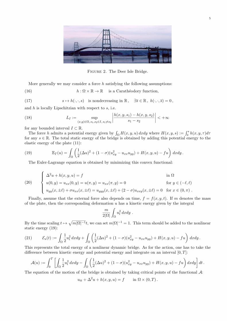
where Υ is the characteristic function of (−ℓ,−ℓ+ε)∪(ℓ−ε, ℓ) and γ > 0. This choice of h is motivatedby the fact that the action of the hangers is larger around the central part of the bridge x = π/2, thanon its sides x = 0 and x = π where the bridge is supported. This parabolic behavior is a consequenceof the prestressing procedure and appears quite visible in certain bridges such as the Deer Isle Bridge,see Figure 2.

5

Figure 2. The Deer Isle Bridge.

More generally we may consider a force h satisfying the following assumptions:

(16) h : Ω× R → R is a Caratheodory function,

(17) s 7→ h(·, ·, s) is nondecreasing in R , ∃s ∈ R , h(·, ·, s) = 0 ,

and h is locally Lipschitzian with respect to s, i.e.

(18) LI := sup(x,y)∈Ω, s1,s2∈I, s1 6=s2

∣∣∣∣h(x, y, s1)− h(x, y, s2)

s1 − s2

∣∣∣∣ < +∞

for any bounded interval I ⊂ R.The force h admits a potential energy given by

∫ΩH(x, y, u) dxdy where H(x, y, s) :=

∫ ss h(x, y, τ)dτ

for any s ∈ R. The total static energy of the bridge is obtained by adding this potential energy to theelastic energy of the plate (11):

(19) ET (u) =

∫

Ω

(1

2(∆u)2 + (1− σ)(u2xy − uxxuyy) +H(x, y, u)− fu

)dxdy .

The Euler-Lagrange equation is obtained by minimizing this convex functional:

(20)

∆2u+ h(x, y, u) = f in Ω

u(0, y) = uxx(0, y) = u(π, y) = uxx(π, y) = 0 for y ∈ (−ℓ, ℓ)uyy(x,±ℓ) + σuxx(x,±ℓ) = uyyy(x,±ℓ) + (2− σ)uxxy(x,±ℓ) = 0 for x ∈ (0, π) .

Finally, assume that the external force also depends on time, f = f(x, y, t). If m denotes the massof the plate, then the corresponding deformation u has a kinetic energy given by the integral

m

2|Ω|

∫

Ωu2t dxdy .

By the time scaling t 7→√m|Ω|−1t, we can set m|Ω|−1 = 1. This term should be added to the nonlinear

static energy (19):

(21) Eu(t) :=∫

Ω

1

2u2t dxdy +

∫

Ω

(1


)dxdy .

This represents the total energy of a nonlinear dynamic bridge. As for the action, one has to take thedifference between kinetic energy and potential energy and integrate on an interval [0, T ]:

A(u) :=

∫ T

0

[∫

Ω

1

2u2t dxdy −

∫

Ω

(1


)dxdy

]dt .

The equation of the motion of the bridge is obtained by taking critical points of the functional A:

utt +∆2u+ h(x, y, u) = f in Ω× (0, T ) .


Due to internal friction, we add a damping term and obtain(22)

utt+δut+∆2u+h(x, y, u)=f in Ω×(0, T )u(0, y, t)=uxx(0, y, t)=u(π, y, t)=uxx(π, y, t)=0 for (y, t)∈(−ℓ, ℓ)×(0, T )uyy(x,±ℓ, t)+σuxx(x,±ℓ, t)=uyyy(x,±ℓ, t)+(2− σ)uxxy(x,±ℓ, t)=0 for (x, t)∈(0, π)×(0, T )u(x, y, 0)=u0(x, y) , ut(x, y, 0)=u1(x, y) for (x, y)∈Ω

where δ is a positive constant. Notice that this equation also arises in different contexts, see e.g. [9,(17)], and is sometimes called the Swift-Hohenberg equation.

3. Main results

Our first purpose is to minimize the energy functional ET , defined in (11), on the space

H2∗ (Ω) :=

w ∈ H2(Ω); w = 0 on 0, π × (−ℓ, ℓ)

.

We also define

H(Ω) := the dual space of H2∗ (Ω)

and we denote by 〈·, ·〉 the corresponding duality. Since we are in the plane, H2(Ω) ⊂ C0(Ω) so thatthe condition on 0, π × (−ℓ, ℓ) introduced in the definition of H2

∗ (Ω) is satisfied pointwise and

(23) Lp(Ω) ⊂ H(Ω) ∀1 6 p 6 ∞ .

If f ∈ L1(Ω) then the functional ET is well-defined in H2∗ (Ω), while if f ∈ H(Ω) we need to replace∫

Ω fu with 〈f, u〉 although we will not mention this in the sequel. The first somehow standard statementis the connection between minimizers of the energy function ET and solutions of (14). It shows thatthe variational setting is correct and it allows to derive the boundary conditions.

Theorem 1. Assume (9) and let f ∈ H(Ω). Then there exists a unique u ∈ H2∗ (Ω) such that

(24)

∫

Ω[∆u∆v + (1− σ)(2uxyvxy − uxxvyy − uyyvxx)] dxdy = 〈f, v〉 ∀v ∈ H2

∗ (Ω) ;

moreover, u is the minimum point of the convex functional ET . Finally, if f ∈ L2(Ω) then u ∈ H4(Ω),and if u ∈ C4(Ω) then u is a classical solution of (14).

Since we have in mind a long narrow rectangle, that is ℓ ≪ π, it is reasonable to assume that theforcing term does not depend on y. So, we now assume that

(25) f = f(x) , f ∈ L2(0, π).

In this case, we may solve (14) following [23, Section 2.2] although the boundary conditions (13) requiresome additional effort. A similar procedure can be used also for some forcing terms depending on ysuch as e±yf(x) or yf(x), see [23]. We extend the source f as an odd 2π-periodic function over R andwe expand it in Fourier series

(26) f(x) =

+∞∑

m=1

βm sin(mx) , βm =2

π

∫ π

0f(x) sin(mx) dx ,

so that βm ∈ ℓ2 and the series converges in L2(0, π) to f . Then we define the constants

(27) A = A(m, ℓ) :=σ

1− σ

βmm4

(1 + σ) sinh(mℓ)− (1− σ)mℓ cosh(mℓ)

(3 + σ) sinh(mℓ) cosh(mℓ)− (1− σ)mℓ,

(28) B = B(m, ℓ) := σβmm4

sinh(mℓ)

(3 + σ) sinh(mℓ) cosh(mℓ)− (1− σ)mℓ,

and we prove

7

Theorem 2. Assume (9) and that f satisfies (25)-(26). Then the unique solution of (14) is given by

u(x, y) =

+∞∑

m=1

[βmm4

+A cosh(my) +Bmy sinh(my)

]sin(mx)

where the constants A and B are defined in (27) and (28).

When ℓ → 0, the plate Ω tends to become a one dimensional beam of length π. We wish to analyzethe behavior of the solution and of the energy in this limit situation. To this end, we re-introduce theconstants appearing in (10) that were normalized in (11). Let f ∈ L2(Ω) be as in (25) and let uℓ be asolution of the problem

(29)

E d3

12(1−σ2)∆2uℓ = f in Ω

uℓ(0, y) = uℓxx(0, y) = uℓ(π, y) = uℓxx(π, y) = 0 for y ∈ (−ℓ, ℓ)uℓyy(x,±ℓ) + σuℓxx(x,±ℓ) = uℓyyy(x,±ℓ) + (2− σ)uℓxxy(x,±ℓ) = 0 for x ∈ (0, π)

whose total energy is given by (10). Obviously, uℓ = 12(1−σ2)Ed3

u, where u is the unique solution of (14)found in Theorem 2. If we view the plate as a parallelepiped-shaped beam (0, π)× (ℓ, ℓ)× (−d/2, d/2)we are led to the problem

(30) EIψ′′′′ = 2ℓf in (0, π) , ψ(0) = ψ′′(0) = ψ(π) = ψ′′(π) = 0 .

Here the forcing term 2ℓf represents a force per unit of length and I = d3ℓ6 =

∫(−ℓ,ℓ)×(−d/2,d/2) z

2dydz is

the moment of inertia of the section of the beam with respect to its middle line parallel to the y-axis.

Then (30) reduces to Ed3

12 ψ′′′′ = f , the function ψ is independent of ℓ but the corresponding total energy

of the beam depends on ℓ:

ET (ψ) =E d3ℓ

12

∫ π

0(ψ′′(x))2dx− 2ℓ

∫ π

0f(x)ψ(x) dx = −

(6π

E d3

+∞∑

m=1

β2mm4

)ℓ .

Then we prove

Theorem 3. Assume (9) and let f ∈ L2(Ω) be a vertical load per unit of surface depending only on x,see (25)-(26). Let uℓ and ψ be respectively as in (29) and (30). Then

(31) limℓ→0

sup(x,y)∈Ω

∣∣∣uℓ(x, y)− ψ(x)∣∣∣ = 0 and ET (u

ℓ) = ET (ψ) + o(ℓ) as ℓ→ 0 .

Theorem 3 states that, when ℓ→ 0, the solution and the energy of the plate are “almost the same” asfor the beam. However, one cannot neglect the o(ℓ) term if one wishes to display torsional oscillations.Next, we study the oscillating modes of the rectangular plate; we consider the eigenvalue problem

(32)

∆2w = λw in Ω

w(0, y) = wxx(0, y) = w(π, y) = wxx(π, y) = 0 for y ∈ (−ℓ, ℓ)wyy(x,±ℓ) + σwxx(x,±ℓ) = wyyy(x,±ℓ) + (2− σ)wxxy(x,±ℓ) = 0 for x ∈ (0, π) .

Similar to (24), problem (32) admits the following variational formulation: a nontrivial function w ∈H2

∗ (Ω) is an eigenfunction of (32) if∫

Ω[∆w∆v + (1− σ)(2wxyvxy − wxxvyy − wyyvxx)− λwv] dxdy = 0 for all v ∈ H2

∗ (Ω) .

In such a case we say that λ is an eigenvalue for problem (32).In Section 7 we prove that for all ℓ > 0 and σ ∈ (0, 12) there exists a unique µ1 ∈ (1− σ, 1) such that

(33)√1− µ1

(µ1 + 1− σ

)2tanh(ℓ

√1− µ1) =

√1 + µ1

(µ1 − 1 + σ

)2tanh(ℓ

√1 + µ1) .

The number λ = µ21 is the least eigenvalue.


Theorem 4. Assume (9). Then the set of eigenvalues of (32) may be ordered in an increasing sequenceλk of strictly positive numbers diverging to +∞ and any eigenfunction belongs to C∞(Ω). The set ofeigenfunctions of (32) is a complete system in H2

∗ (Ω).Moreover, the least eigenvalue of (32) is λ1 = µ21, where µ1 ∈ (1 − σ, 1) is the unique solution of

(33); the least eigenvalue µ21 is simple and the corresponding eigenspace is generated by the positiveeigenfunction[µ1 + 1− σ] cosh(

√1 + µ1ℓ) cosh(

√1− µ1y) + [µ1 − 1 + σ] cosh(

√1− µ1ℓ) cosh(

√1 + µ1y)

sinx

defined for any (x, y) ∈ Ω.

In fact, we obtain a stronger statement describing the whole spectrum and characterizing the eigen-functions, see Theorem 15 in Section 7. In Proposition 16 we also show that if ℓ is small enough(ℓ 6 0.44), then the first two eigenvalues are simple. In Figure 3 we display the qualitative behavior ofthe first two ”longitudinal” eigenfunctions and of the first two ”torsional” eigenfunctions. It appears

Figure 3. Qualitative behavior of some eigenfunctions of (32).

that the maximum and minimum of these eigenfunctions are attained on the boundary and that everymode has a tendency to display a torsional behavior: as expected, the “weak” part of the plate arethe two long free edges. Note also that in the limit case σ = 0, excluded by assumption (9), the firsteigenvalue is λ1 = 1 and the first eigenfunction is sinx.We now turn to the nonlinear model. With a simple minimization argument one can prove

Theorem 5. Assume (9), (16)-(18) and let f ∈ H(Ω); then there exists a unique weak solution u ∈H2

∗ (Ω) of (20). This solution is the unique minimizer of the problem

minv∈H2

∗(Ω)

ET (v)

where ET is the nonlinear static energy defined in (19).

Since the proof of Theorem 5 is standard, we omit it.Our last result proves well-posedness for the evolution problem (22). If T > 0 we say that

(34) u ∈ C0([0, T ];H2∗ (Ω)) ∩ C1([0, T ];L2(Ω)) ∩ C2([0, T ];H(Ω))

is a solution of (22) if it satisfies the initial conditions and if

(35)〈u′′(t), v〉+ δ(u′(t), v)L2 + (u(t), v)H2

∗

+ (h(·, ·, u(t)), v)L2 = (f(t), v)L2

∀v ∈ H2∗ (Ω) , ∀t ∈ (0, T ) .

If T = +∞ then the interval [0, T ] should be read as [0,+∞). Then we have

Theorem 6. Assume (9), (16)-(18). Let T > 0 (including the case T = +∞), let f ∈ C0([0, T ];L2(Ω))and let δ > 0; let u0 ∈ H2

∗ (Ω) and u1 ∈ L2(Ω). Then

(i) there exists a unique solution of (22);(ii) if f ∈ L2(Ω) is independent of t, then T = +∞ and the unique solution u of (22) satisfies

u(t) → u in H2∗ (Ω) and u′(t) → 0 in L2(Ω) as t→ +∞

where u is the unique solution of the stationary problem (20).

9

4. Proof of Theorem 1

Let D2w denote the Hessian matrix of a function w ∈ H2(Ω). Thanks to the Intermediate DerivativesTheorem, see [1, Theorem 4.15], the space H2(Ω) is a Hilbert space if endowed with the scalar product

(u, v)H2 :=

∫

Ω

(D2u ·D2v + uv

)dxdy for all u, v ∈ H2(Ω) .

On the closed subspace H2∗ (Ω) we may also define a different scalar product.

Lemma 7. Assume (9). On the space H2∗ (Ω) the two norms

u 7→ ‖u‖H2 , u 7→ ‖u‖H2∗

:=

[∫

Ω

[(∆u)2 + 2(1− σ)(u2xy − uxxuyy)

]dxdy

]1/2

are equivalent. Therefore, H2∗ (Ω) is a Hilbert space when endowed with the scalar product

(36) (u, v)H2∗

:=

∫

Ω[∆u∆v + (1− σ)(2uxyvxy − uxxvyy − uyyvxx)] dxdy .

Proof. We first get rid of the L2-norm. Take any u ∈ H2∗ (Ω) so that u ∈ C0(Ω) and for all (x, y) ∈ Ω

we have

|u(x, y)| =

∣∣∣∣∫ x

0ux(t, y)dt

∣∣∣∣ 6∫ π

0|ux(t, y)|dt 6

√π

[∫ π

0(ux(t, y))

2dt

]1/2

6√π

[−∫ π

0uxx(t, y)u(t, y)dt

]1/26

√π

[∫ π

0(uxx(t, y))

2dt

]1/4 [∫ π

0(u(t, y))2dt

]1/4

where we used an integration by parts and twice Holder’s inequality. This inequality, readily yields‖u‖L2 6 C‖D2u‖L2 for some C > 0 and proves that the H2(Ω)-norm is equivalent to the normu 7→ ‖D2u‖L2 on the space H2

∗ (Ω). Next, we notice that

(1− σ)‖D2u‖2L2 6 ‖u‖2H2∗

=

∫

Ω[u2xx + u2yy + 2(1− σ)u2xy + 2σuxxuyy]dxdy 6 (1 + σ)‖D2u‖2L2

so that the norms u 7→ ‖D2u‖L2 andH2∗ (Ω) are equivalent. These two equivalences prove the lemma.

By combining Lemma 7 with the Lax-Milgram Theorem, we infer that for any f ∈ H(Ω) there existsa unique u ∈ H2

∗ (Ω) satisfying (24). This proves the first part of Theorem 1.

Our next purpose is to study the regularity of the just found solution of (24).

Lemma 8. Assume (9) and 1 < p <∞; let f ∈ Lp(Ω) and let u ∈ H2∗ (Ω) be a (weak) solution of (14).

Then u ∈W 4,p(Ω) and there exists a constant C(ℓ, σ, p) depending only on ℓ, σ and p such that

(37) ‖u‖W 4,p 6 C(ℓ, σ, p)‖f‖Lp .

Proof. By (23) and Lemma 7, the assumptions make sense. The next step is to show that the boundaryconditions satisfy the complementing conditions, see [2, p.633] for the definition. On the vertical edgeswe have Navier boundary conditions for which this property is well-known, see [11, Section 2.3]. On thehorizontal edges, the polynomials R2 → R in the variables α, β associated to the boundary conditions(13) are independent of x and y and read B1(α, β) = σα2 + β2 and B2(α, β) = (2 − σ)α2β + β3. Letν = (ν1, ν2) denote the unit normal to ∂Ω and let τ = (τ1, τ2) be any vector tangent to ∂Ω so thatν1 = τ2 = 0 and ν2 = sign y while τ1 is arbitrary. Then B1(τ + tν) = t2 + στ21 and B2(τ + tν) =(sign y)t[t2 + (2− σ)τ21 ]; therefore

B1(x, y, τ + tν) = 2i|τ1|t+ (σ + 1)τ21 mod (t− i|τ |)2 ,B2(x, y, τ + tν) = (sign y)

[−(σ + 1)τ21 t+ 2i|τ1|3

]mod (t− i|τ |)2 .

Since σ 6= 1, the polynomials

B1(t) := 2i|τ1|t+ (σ + 1)τ21 and B2(t) := (sign y)[−(σ + 1)τ21 t+ 2i|τ1|3

]


are linearly independent: indeed,

−(sign y)(σ + 1)|τ1|2i

B1(t) = (sign y)

[−(σ + 1)τ21 t+ i

(σ + 1)2|τ1|32

]

with (σ+1)2

2 6= 2. This proves that also (13) satisfies the complementing conditions.The lack of smoothness of ∂Ω is not a serious difficulty. By odd extension, we can view the problem

in Ω as the restriction of a problem in (−π, 2π)× (−ℓ, ℓ). Then classical elliptic local regularity results[2, Theorem 15.1] yield (37). We also refer to [24] for more general regularity results in nonsmoothdomains.

Finally, we show that smooth weak solutions and classical solutions coincide. Note first that, for allu ∈ H2

∗ (Ω) we have

(38) u(0, y) = u(π, y) = uy(0, y) = uy(π, y) = uyy(0, y) = uyy(π, y) = 0 for y ∈ (−ℓ, ℓ) .Then, by adapting the Gauss-Green formula

∫

Ω∆u∆v dx dy =

∫

Ω∆2uv dx dy +

∫

∂Ω

[∆u vν − v (∆u)ν

]ds

to our situation, and with some integration by parts, we obtain that if u ∈ C4(Ω) ∩ H2∗ (Ω) satisfies

(24), then∫

Ω(∆2u− f)v dxdy +

∫ ℓ

−ℓ[uxx(π, y)vx(π, y)− uxx(0, y)vx(0, y)] dy(39)

+

∫ π

0

[uyyy(x,−ℓ) + (2− σ)uxxy(x,−ℓ)] v(x,−ℓ)− [uyy(x,−ℓ) + σuxx(x,−ℓ)] vy(x,−ℓ)

dx

+

∫ π

0

[uyy(x, ℓ) + σuxx(x, ℓ)] vy(x, ℓ)− [uyyy(x, ℓ) + (2− σ)uxxy(x, ℓ)] v(x, ℓ)

dx = 0

for any v ∈ H2∗ (Ω). If we choose v ∈ C2

c (Ω) in (39), then all the boundary terms vanish and we deducethat ∆2u = f in Ω. Hence we may drop the double integral in (39). By arbitrariness of v, the coefficientsof the terms vx(π, y), vx(0, y), v(x,−ℓ), vy(x,−ℓ), vy(x, ℓ), and v(x, ℓ) must vanish identically and weobtain (12)-(13); this conclusion may also be reached with particular choices of v but we omit here thetedious computations.We have so proved that if u ∈ C4(Ω)∩H2

∗ (Ω) satisfies (24) then it is a classical solution of (14). Forthe converse implication let u ∈ C4(Ω) be a classical solution of (14) and let v ∈ H2

∗ (Ω). Then (39)holds true and moreover exploiting (38) and integrating by parts we also recover the validity of (24)for all v ∈ H2

∗ (Ω).


Consider the function

(40) φ(x) :=+∞∑

m=1

βmm4

sin(mx)

and note that it solves the ODE

φ′′′′(x) = f(x) in (0, π) , φ(0) = φ′′(0) = φ(π) = φ′′(π) = 0 .

Moreover, φ′′ ∈ H2(0, π) is given by

(41) φ′′(x) = −+∞∑

m=1

βmm2

sin(mx)

and the series (41) converges in H2(0, π) and, hence, uniformly.

11

We now introduce the auxiliary function v(x, y) := u(x, y)− φ(x); if u solves (14), then v satisfies

(42)

∆2v = 0 in Ω

v = vxx = 0 on 0, π × (−ℓ, ℓ)vyy + σvxx = −σφ′′ on (0, π)× −ℓ, ℓvyyy + (2− σ)vxxy = 0 on (0, π)× −ℓ, ℓ .

We seek solutions of (42) by separating variables, namely we seek functions Ym = Ym(y) such that

v(x, y) =

+∞∑

m=1

Ym(y) sin(mx)

solves (42). Then

∆2v(x, y) =

+∞∑

m=1

[Y ′′′′m (y)− 2m2Y ′′

m(y) +m4Ym(y)] sin(mx)

and the equation in (42) yields

(43) Y ′′′′m (y)− 2m2Y ′′

m(y) +m4Ym(y) = 0 for y ∈ (−ℓ, ℓ) .

The solutions of (43) are linear combinations of cosh(my), sinh(my), y cosh(my), y sinh(my) but, dueto the symmetry of Ω and to the uniqueness of the solution v to (42), we know that Ym is even withrespect to y. Hence, we seek functions Ym of the form

(44) Ym(y) = A cosh(my) +Bmy sinh(my)

where A = A(m, ℓ) and B = B(m, ℓ) are constants to be determined by imposing the boundaryconditions in (42) and the coefficient m is highlighted on the term y sinh(my) for later simplifications.By differentiating we obtain

Y ′m(y) = m[(A+B) sinh(my) +Bmy cosh(my)] , Y ′′

m(y) = m2[(A+ 2B) cosh(my) +Bmy sinh(my)] ,

(45) Y ′′′m (y) = m3[(A+ 3B) sinh(my) +Bmy cosh(my)] .

The two boundary conditions on (0, π)× −ℓ, ℓ, see (42), become respectively

+∞∑

m=1

[Y ′′m(±ℓ)− σm2Ym(±ℓ)] sin(mx) = −σφ′′(x) ,

+∞∑

m=1

[Y ′′′m (±ℓ)− (2− σ)m2Y ′

m(±ℓ)] sin(mx) = 0 ,

for all x ∈ (0, π), and, by (41),

Y ′′m(ℓ)− σm2Ym(ℓ) = σ

βmm2

, Y ′′′m (ℓ)− (2− σ)m2Y ′

m(ℓ) = 0 ,

the condition for y = −ℓ being automatically fulfilled since Ym is even. By plugging these informationinto the explicit form (45) of the derivatives we find the system

(1− σ) cosh(mℓ)A+(2 cosh(ml) + (1− σ)mℓ sinh(mℓ)

)B = σ βm

m4

(1− σ) sinh(mℓ)A+((1− σ)mℓ cosh(mℓ)− (1 + σ) sinh(mℓ)

)B = 0 ,

and we finally obtain (27)-(28).



Let u ∈ H2∗ (Ω) be the solution of (14), see Theorem 2. By (27)-(28) we have

|A cosh(my)| 6 Cβmm3

and Bmy sinh(my) 6 Cβmm3

for any y ∈ (−ℓ, ℓ), ℓ ∈ (0, 1) and m > 1 for some constant C > 0 depending on σ but independent ofy, ℓ and m. Moreover we also have

(46) limℓ→0

A(m, ℓ) =σ2

1− σ2βmm4

, limℓ→0

B(m, ℓ) =σ

2(1 + σ)

βmm4

for any m ∈ N .

This implies that for any N ∈ N

lim supℓ→0

sup(x,y)∈Ω

∣∣∣∣u(x, y)−1

1− σ2φ(x)

∣∣∣∣6lim supℓ→0

supy∈(−ℓ,ℓ)

+∞∑

m=1

∣∣∣∣A cosh(my)− σ2

1− σ2βmm4

+Bmy sinh(my)

∣∣∣∣

6 limℓ→0

N∑

m=1

[∣∣∣∣A− σ2

1− σ2βmm4

∣∣∣∣ cosh(mℓ) +σ2

1− σ2βmm4

(cosh(mℓ)− 1) +Bmℓ sinh(mℓ)

]+ C

+∞∑

m=N+1

βmm3

6 C+∞∑

m=N+1

βmm3

.

Letting N → +∞, we obtain

(47) limℓ→0

sup(x,y)∈Ω

∣∣∣∣u(x, y)−1

1− σ2φ(x)

∣∣∣∣ = 0 .

Let us now recall a well-known result about Fourier series which will be repeatedly used in the sequel.

Lemma 9. Let am, bm ∈ ℓ2 and let

a(x) =

+∞∑

m=1

am sin(mx) , b(x) =

+∞∑

m=1

bm sin(mx) .

Then a, b ∈ L2(0, π) and

∫ π

0a(x)b(x) dx =

π

2

+∞∑

m=1

ambm ,

∫ π

0a(x)2 dx =

π

2

+∞∑

m=1

a2m .

By differentiating the solution u we find

uxx(x, y) = −+∞∑

m=1

[βmm2

+Am2 cosh(my) +Bm3y sinh(my)

]sin(mx) ,

uyy(x, y) =

+∞∑

m=1

m2[(A+ 2B) cosh(my) +Bmy sinh(my)] sin(mx) ,

uxy(x, y) =+∞∑

m=1

m2[(A+B) sinh(my) +Bmy cosh(my)] cos(mx) ,

and therefore

∆u(x, y) =+∞∑

m=1

[−βmm2

+ 2Bm2 cosh(my)

]sin(mx) .

13

Then, by Lemma 9, we obtain

∫

Ω|∆u|2 =

π

2

+∞∑

m=1

∫ ℓ

−ℓ

[−βmm2

+ 2Bm2 cosh(my)

]2dy(48)

= π+∞∑

m=1

[β2mm4

ℓ+ 2B2m4ℓ− 4Bβmm

sinh(mℓ) +B2m3 sinh(2mℓ)

].

Moreover, Lemma 9 also yields

∫

Ωuxxuyy = −π

2

+∞∑

m=1

∫ ℓ

−ℓ[βm +Am4 cosh(my) +Bm5y sinh(my)](49)

×[(A+ 2B) cosh(my) +Bmy sinh(my)] dy

= −π+∞∑

m=1

[βm

m [(A+B) sinh(mℓ) +Bmℓ cosh(mℓ)] + B(2A+B)m3

4 mℓ cosh(2mℓ)

+(2A2+2AB−B2

8 + B2

4 m2ℓ2)m3 sinh(2mℓ) + A(A+2B)

2 m4ℓ− B2

6 m6ℓ3]

and∫

Ωu2xy =

π

2

+∞∑

m=1

m4

∫ ℓ

−ℓ[(A+B) sinh(my) +Bmy cosh(my)]2 dy(50)

= π+∞∑

m=1

m3[2A2+2AB+B2

8 sinh(2mℓ) + B(2A+B)4 mℓ cosh(2mℓ) + B2

4 m2ℓ2 sinh(2mℓ)

+B2

6 m3ℓ3 − (A+B)2

2 mℓ].

Finally, by (26) and a further application of Lemma 9,

∫

Ωfu =

π

2

+∞∑

m=1

βm

∫ ℓ

−ℓ

[βm

m4 +A cosh(my) +Bmy sinh(my)]dy(51)

= π+∞∑

m=1

βm

[βm

m4 ℓ+A−Bm sinh(mℓ) +Bℓ cosh(mℓ)

].

Collecting (48)-(51) we obtain

ET (u)=π

+∞∑

m=1

−β

2mℓ

2m4+σ + 1

2B2m4ℓ−σβm(A+B)

msinh(mℓ) +

B2m3

2sinh(2mℓ)− σβmBℓ cosh(mℓ)

+1− σ

2

[A(A+B)m3 sinh(2mℓ)+B2m5ℓ2 sinh(2mℓ)+B(2A+B)m4ℓ cosh(2mℓ)

]=:

+∞∑

m=1

a(m, ℓ) .

With a direct computation one can see that by (27) and (28) we get

|a(m, ℓ)|ℓ

6 Cβ2mm3

for any ℓ ∈ (0, 1) and m > 1

for some constant C > 0 depending on σ but independent of ℓ and m.This implies that for any N ∈ N we have

N∑

m=1

a(m, ℓ)

ℓ−

+∞∑

m=N+1

Cβ2mm3

6

+∞∑

m=1

a(m, ℓ)

ℓ6

N∑

m=1

a(m, ℓ)

ℓ+

+∞∑

m=N+1

Cβ2mm3

.


Letting ℓ→ 0 we obtain

N∑

m=1

limℓ→0

(a(m, ℓ)

ℓ

)−

+∞∑

m=N+1

Cβ2mm3

6 lim infℓ→0

+∞∑

m=1

a(m, ℓ)

ℓ

6 lim supℓ→0

+∞∑

m=1

a(m, ℓ)

ℓ6

N∑

m=1

limℓ→0

(a(m, ℓ)

ℓ

)+

+∞∑

m=N+1

Cβ2mm3

.

Letting N → +∞, by (46), we deduce that

limℓ→0

ET (u)

ℓ= lim

ℓ→0

+∞∑

m=1

a(m, ℓ)

ℓ=

+∞∑

m=1

limℓ→0

a(m, ℓ)

ℓ= − π

2(1− σ2)

+∞∑

m=1

β2mm4

and, in turn,

(52) ET (u) = −(

π

2(1− σ2)

+∞∑

m=1

β2mm4

)ℓ+ o(ℓ) as ℓ→ 0 .

Consider now uℓ and ψ as in (29) and (30); recall that uℓ = 12(1−σ2)Ed3

u where u solves (14) and that

ψ = 12Ed3

φ. Then, from (47) we deduce the first of (31). Moreover, from (52) we obtain

ET (uℓ) =

12(1− σ2)

E d3

∫

Ω

[1

2(∆uℓ)2 + (σ − 1)det(D2uℓ)− fuℓ

]dxdy

=12(1− σ2)

E d3

[−(

π

2(1− σ2)

+∞∑

m=1

β2mm4

)ℓ+ o(ℓ)

]

and the second of (31) follows.


By Lemma 7 the bilinear form (36) is continuous and coercive; standard spectral theory then showsthat the eigenvalues of (32) may be ordered in an increasing sequence of strictly positive numbersdiverging to +∞ and that the corresponding eigenfunctions form a complete system in H2

∗ (Ω). Theeigenfunctions are smooth in Ω: this may be obtained by making an odd extension as in Lemma 8 andwith a bootstrap argument. This proves the first part of Theorem 4.Take an eigenfunction w of (32) and consider its Fourier expansion with respect to the variable x:

(53) w(x, y) =

+∞∑

m=1

hm(y) sin(mx) for (x, y) ∈ (0, π)× (−ℓ, ℓ) .

Since w ∈ C∞(Ω), the Fourier coefficients hm = hm(y) are smooth functions and solve the ordinarydifferential equation

(54) h′′′′m (y)− 2m2h′′m(y) + (m4 − λ)hm(y) = 0

for some λ > 0. The eigenfunction w in (53) satisfies (12), while by imposing (13) we obtain theboundary conditions on hm

(55) h′′m(±ℓ)− σm2hm(±ℓ) = 0 , h′′′m(±ℓ) + (σ − 2)m2h′m(±ℓ) = 0 .

Put µ =√λ > 0 and consider the characteristic equation α4 − 2m2α2 +m4 − µ2 = 0 related to (54).

By solving this algebraic equation we find

(56) α2 = m2 ± µ .

Three cases have to be distinguished.• The case 0 < µ < m2. By (56) we infer

(57) α = ±β or α = ±γ with√m2 − µ =: γ < β :=

√m2 + µ .

15

Hence, possible nontrivial solutions of (54)-(55) have the form

(58) hm(y) = a cosh(βy) + b sinh(βy) + c cosh(γy) + d sinh(γy) (a, b, c, d ∈ R) .

By computing the derivatives of hm and imposing the conditions (55) we find the two systems

(59)

(β2 −m2σ) cosh(βℓ)a+ (γ2 −m2σ) cosh(γℓ)c = 0

(β3 −m2(2− σ)β) sinh(βℓ)a+ (γ3 −m2(2− σ)γ) sinh(γℓ)c = 0 ,

(β2 −m2σ) sinh(βℓ)b+ (γ2 −m2σ) sinh(γℓ)d = 0

(β3 −m2(2− σ)β) cosh(βℓ)b+ (γ3 −m2(2− σ)γ) cosh(γℓ)d = 0 .

There exists a nontrivial solution hm of (54) of the form (58) if and only if there exists a nontrivialsolution of at least one of the two systems (59). The first system in (59) admits a nontrivial solution(a, c) if and only if

(β2 −m2σ)(γ3 −m2(2− σ)γ) cosh(βℓ) sinh(γℓ) = (γ2 −m2σ)(β3 −m2(2− σ)β) sinh(βℓ) cosh(γℓ) .

By (57), this is equivalent to

(60)γ

(γ2 −m2σ)2tanh(ℓγ) =

β

(β2 −m2σ)2tanh(ℓβ) .

Recalling that both β and γ depend on µ, we prove

Lemma 10. Assume (9). For any m > 1 there exists a unique µ = µm ∈ (0,m2) such that (60) holds;moreover we also have µm ∈ ((1− σ)m2,m2).

Proof. Consider the function ηm(t) := t(t2−m2σ)2

· tanh(ℓt) for any t ∈ [0,+∞) \ √σm. Then

η′m(t) =(−3t2 −m2σ) sinh(ℓt) cosh(ℓt) + ℓt(t2 −m2σ)

(t2 −m2σ)3 cosh2(ℓt)∀t ∈ [0,+∞) \

√σm .

For any t >√σm we have

η′m(t) <−3t2 sinh(ℓt) cosh(ℓt) + ℓt3

(t2 −m2σ)3 cosh2(ℓt)< − 2ℓt3

(t2 −m2σ)3 cosh2(ℓt)< 0 .

This shows that ηm is decreasing in (√σm,+∞) and, if β > γ >

√σm then ηm(β) < ηm(γ) so that

(60) cannot hold. We have proved that if γ and β satisfy (60) then necessarily γ ∈ [0,√σm).

Since β =√

2m2 − γ2, identity (60) is equivalent to

(61)

√2m2 − γ2 (γ2 −m2σ)2

[(2− σ)m2 − γ2]2tanh(ℓ

√2m2 − γ2) = γ tanh(ℓγ) .

Then we define

gm(t) :=

√2m2 − t2 (m2σ − t2)2

[(2− σ)m2 − t2]2tanh(ℓ

√2m2 − t2) ∀t ∈ [0,

√σm] .

The function t 7→ [m2σ − t2]/[(2− σ)m2 − t2] is nonnegative and decreasing and hence so is its square.It then follows that gm is decreasing in [0,

√σm] and gm(

√σm) = 0. On the other hand, the map

t 7→ t tanh(ℓt) is increasing in [0,√σm] and vanishes at t = 0. This proves that there exists a unique

γm ∈ (0,√σm) satisfying (61). The statements of the lemma now follow by putting µm = m2−γ2m.

In the next result we prove that the sequence µm found in Lemma 10 is increasing.

Lemma 11. Assume (9). For any m > 1, let µm be as in Lemma 10. Then µm < µm+1 for all m > 1.


Proof. By (57), the equation (60) reduces to

(62) Φ(m,µ) :=

√m2 − µ

m2 + µ

(µ+ (1− σ)m2

µ− (1− σ)m2

)2tanh(ℓ

√m2 − µ)

tanh(ℓ√m2 + µ)

= 1 .

We consider Φ as a function defined in the region of the plane (m,µ) ∈ R2; (1− σ)m2 < µ < m2. In

this region, the three maps

(m,µ) 7→√m2 − µ

m2 + µ, (m,µ) 7→

(µ+ (1− σ)m2

µ− (1− σ)m2

)2

, (m,µ) 7→ tanh(ℓ√m2 − µ)

tanh(ℓ√m2 + µ)

,

are all positive, strictly increasing with respect to m, and strictly decreasing with respect to µ. There-fore, the function m 7→ µm, implicitly defined by Φ(m,µm) = 1, is strictly increasing.

Similarly, the second system in (59) has nontrivial solutions (b, d) if and only if

(β2 −m2σ)(γ3 −m2(2− σ)γ) sinh(βℓ) cosh(γℓ) = (γ2 −m2σ)(β3 −m2(2− σ)β) cosh(βℓ) sinh(γℓ) .

By (57), this is equivalent to

(63)β

(β2 −m2σ)2coth(ℓβ) =

γ

(γ2 −m2σ)2coth(ℓγ) .

Recalling that both β and γ depend on µ, we prove

Lemma 12. Assume (9). Then there exists a unique µ = µm ∈ (0,m2) satisfying (63) if and only if

(64) ℓm√2 coth(ℓm

√2) >

(2− σ

σ

)2

.

Moreover in such a case we have µm ∈ ((1− σ)m2,m2).

Proof. The function ηm(t) := t(t2−m2σ)2

· coth(ℓt) is strictly decreasing for t ∈ (√σm,+∞) because it

is the product of two positive and strictly decreasing functions. In particular, if β > γ >√σm then

ηm(β) < ηm(γ) so that (63) cannot hold. This proves that if γ and β satisfy (63) then necessarilyγ ∈ (0,

√σm).

By (57) identity (63) is equivalent to

(65)

√2m2 − γ2 (γ2 −m2σ)2

[(2− σ)m2 − γ2]2coth(ℓ

√2m2 − γ2) = γ coth(ℓγ) .

Then we define

(66) gm(t) =

√2m2 − t2 (m2σ − t2)2

[(2− σ)m2 − t2]2coth(ℓ

√2m2 − t2) ∀t ∈ [0,

√σm] .

We have

g′m(t) =ℓt(m2σ − t2)2

[(2− σ)m2 − t2]2 sinh2(ℓ√2m2 − t2)

(67)

− 8(1− σ)m2(2m2 − t2) + (m2σ − t2)[(2− σ)m2 − t2]√2m2 − t2 [(2− σ)m2 − t2]3

(m2σ − t2) t coth(ℓ√

2m2 − t2)

<t(m2σ − t2)2 [(2− σ)m2 − t2][ℓ

√2m2 − t2 − sinh(ℓ

√2m2 − t2) cosh(ℓ

√2m2 − t2)]√

2m2 − t2[(2− σ)m2 − t2]3 sinh2(ℓ√2m2 − t2)

< 0

for any t ∈ (0,√σm). Therefore gm is decreasing in (0,

√σm) with gm(0) =

√2m( σ

2−σ )2 coth(ℓm

√2)

and gm(√σm) = 0. On the other hand, the map t 7→ t coth(ℓt) is increasing in (0,

√σm) and tends to

1/ℓ as t→ 0+. This proves that there exists a unique γm ∈ (0,√σm) satisfying (65) if and only if (64)

holds. The proof of the lemma now follows by putting µm = m2 − (γm)2.

17

Note also that (64) holds if and only if m is large enough, that is,

(68) ∃mσ > 1 such that (64) holds if and only if m > mσ .

In particular, if ℓ√2 coth(ℓ

√2) > ( σ

2−σ )2 then mσ = 1. We now prove that the sequence µm, found

in Lemma 12, is increasing.

Lemma 13. Assume (9). For any m > 1, let µm as in the statement of Lemma 12. Then µm < µm+1

for any m > mσ, see (68).

Proof. Let m > mσ; by Lemma 12 we know that µm < m2 and µm+1 > (1− σ)(m+1)2. Therefore, wemay restrict our attention to the case where (1−σ)(m+1)2 < m2 and µm, µm+1 ∈ ((1−σ)(m+1)2,m2)since otherwise the statement follows immediately. For

(m,µ) ∈ A := (m,µ) ∈ R2; m > mσ, (1− σ)(m+ 1)2 < µ < m2 ,

consider the functions

Γ(m,µ) :=

√µ+m2 [µ− (1− σ)m2]2

[µ+ (1− σ)m2]2coth(ℓ

√µ+m2) , K(m,µ) :=

√m2 − µ coth(ℓ

√m2 − µ) .

On the interval µ < s < µ1−σ , both the positive maps

s 7→√µ+ s [µ− (1− σ)s]2

[µ+ (1− σ)s]2and s 7→ coth(ℓ

√µ+ s)

have strictly negative derivatives. Moreover, if gm is as in (66), then Γ(m,µ) = gm(√m2 − µ) and (67)

proves that µ 7→ Γ(m,µ) has strictly positive derivative. Summarizing,

(69)∂Γ

∂m(m,µ) < 0 and

∂Γ

∂µ(m,µ) > 0 ∀(m,µ) ∈ A .

It is also straightforward to verify that

(70)∂K

∂m(m,µ) > 0 and

∂K

∂µ(m,µ) < 0 ∀(m,µ) ∈ A .

Finally, put

(71) Ψ(m,µ) :=K(m,µ)

Γ(m,µ)∀(m,µ) ∈ A .

The function m 7→ µm is implicitly defined by Ψ(m,µm) = 1, see (63) and (57). By (69)-(70) we infer

∂Ψ

∂m(m,µ) > 0 and

∂Ψ

∂µ(m,µ) < 0 ∀(m,µ) ∈ A .

This proves that the map m 7→ µm is strictly increasing.

We finally compare µm with µm.

Lemma 14. Assume (9). Let µm and µm be, respectively, as in Lemmas 10 and 12. Then for anym > mσ we have µm < µm.

Proof. Let Φ and Ψ be as in (62) and (71); then Φ(m,µ) < Ψ(m,µ) for all (m,µ) ∈ A. Since µm

is implicitly defined by Ψ(m,µm) = 1, we have Φ(m,µm) < 1. Moreover, in Lemma 11 we saw thatµ 7→ Φ(m,µ) is strictly decreasing. Hence, Φ(m,µm) < 1 = Φ(m,µm) implies µm < µm.

• The case µ = m2. By (56) we infer that possible nontrivial solutions of (54)-(55) have the form

hm(y) = a cosh(√2my) + b sinh(

√2my) + c+ dy (a, b, c, d ∈ R) .


By differentiating hm and by imposing the boundary conditions (55) we get

(72)

(2− σ) cosh(√2mℓ)a− σc = 0

σ sinh(√2mℓ)a = 0 ,

(2− σ) sinh(√2mℓ)b− σℓd = 0

√2mσ cosh(

√2mℓ)b+ (σ − 2)d = 0 .

The first system in (72) has the unique solution a = c = 0 under the assumption (9). The secondsystem in (72) admits a nontrivial solution (b, d) if and only if

(73) tanh(√2mℓ) =

(σ

2− σ

)2 √2mℓ .

By (9) the equation tanh(s) =(

σ2−σ

)2s admits a unique solution s > 0. But if m∗ := s/ℓ

√2 is not an

integer, then (73) admits no solution. If m∗ ∈ N, then the second system in (72) admits a nontrivialsolution (b, d) 6= (0, 0) whenever m = m∗. If m ∈ N does not satisfy (73), then the second system in(72) only admits the trivial solution b = d = 0.• The case µ > m2. By (56) we infer that

(74) α = ±β or α = ±iγ with√µ−m2 = γ < β =

√µ+m2 .

Therefore, possible nontrivial solutions of (54) have the form

hm(y) = a cosh(βy) + b sinh(βy) + c cos(γy) + d sin(γy) (a, b, c, d ∈ R) .

Differentiating hm and imposing the boundary conditions (55) yields the two systems:

(75)

(β2 −m2σ) cosh(βℓ)a− (γ2 +m2σ) cos(γℓ)c = 0

(β3 −m2(2− σ)β) sinh(βℓ)a+ (γ3 +m2(2− σ)γ) sin(γℓ)c = 0 ,

(76)

(β2 −m2σ) sinh(βℓ)b− (γ2 +m2σ) sin(γℓ)d = 0

(β3 −m2(2− σ)β) cosh(βℓ)b− (γ3 +m2(2− σ)γ) cos(γℓ)d = 0 .

Due to the presence of trigonometric sine and cosine, for any integer m there exists a sequenceζmk ↑ +∞ such that ζmk > m2 for all k ∈ N and such that if µ = ζmk for some k then one of the abovesystems admits a nontrivial solution.

Not only the above arguments prove all the statements of Theorem 4, but they also prove the followingresult.

Theorem 15. Assume (9) and consider the eigenvalue problem (32). Then:(i) for any m > 1 there exists a sequence of eigenvalues λk,m ↑ +∞ such that λk,m > m4 for all

k > 1; the corresponding eigenfunctions are of the kind[a cosh

(y

√λ1/2k,m +m2

)+b sinh

(y

√λ1/2k,m +m2

)+c cos

(y

√λ1/2k,m −m2

)+d sin

(y

√λ1/2k,m −m2

)]sin(mx)

for suitable constants a, b, c, d, depending on m and k;(ii) if the unique positive solution m of (73) is an integer m∗ ∈ N, then λ = m4

∗ is an eigenvalue withcorresponding eigenfunction

[σℓ sinh(

√2m∗y) + (2− σ) sinh(

√2m∗ℓ) y

]sin(m∗x) ;

19

(iii) for any m > 1, there exists an eigenvalue λm ∈ ((1−σ)2m4,m4) with corresponding eigenfunction(√λm − (1− σ)m2

) cosh(y√m2 +

√λm

)

cosh(ℓ√m2 +

√λm

) +(√

λm + (1− σ)m2) cosh

(y√m2 −

√λm

)

cosh(ℓ√m2 −

√λm

)

sin(mx) ;

(iv) for any m > 1, satisfying (64), there exists an eigenvalue λm ∈ (λm,m4) with corresponding

eigenfunction(√λm − (1− σ)m2

) sinh(y√m2 +

√λm)

sinh(ℓ√m2 +

√λm) +

(√λm + (1− σ)m2

) sinh(y√m2 −

√λm)

sinh(ℓ√m2 −

√λm)

sin(mx) ;

(v) There are no eigenvalues other than the ones characterized in (i)− (iv).

Note that the eigenfunctions in (iii) are even with respect to y whereas the eigenfunctions in (iv) areodd. In the next result we give a precise description of the first two eigenvalues when ℓ is small enough.

Proposition 16. Assume (9) and consider the eigenvalue problem (32). If ℓ 6 15 then the first two

eigenvalues are simple and they coincide with the numbers λ1, λ2 defined by Lemma 10. Therefore,

(77) (1− σ)2 < λ1 < 1 < 16(1− σ)2 < λ2 < 16 .

Proof. By (9) we know that (64) may hold only if ℓm√2 coth(ℓm

√2) > 9. In turn, since ℓ 6 1

5 , thisnecessarily yields m > 31. From Theorem 15 we readily obtain (77). In order to prove the statementit is therefore enough to show that all the other eigenvalues found in Theorem 15 are larger than orequal to 16 for ℓ 6 1

5 .

We start by showing that for ℓ 6 15 the numbers µ corresponding to the case µ > m2 are larger than

or equal to 4. We take m = 1 since if m > 2 we immediately obtain µ > 4 and we are done.When m = 1 system (75) admits a nontrivial solution if and only if

(β2 − σ)(γ3 + (2− σ)γ) cosh(βℓ) sin(γℓ) + (γ2 + σ)(β3 − (2− σ)β) sinh(βℓ) cos(γℓ) = 0 .

This may happen only if the two terms sin(γℓ) and cos(γℓ) have opposite sign: this yields

γ

5> γℓ >

π

2=⇒ γ >

5π

2=⇒ µ > 1 +

(5π

2

)2

> 4 .

Consider now the system (76) with m = 1. Put

h(µ, σ, ℓ) :=

(µ+ 1− σ)2√µ− 1 sinh(ℓ

√µ+ 1) cos(ℓ

√µ− 1)− (µ− 1 + σ)2

√µ+ 1 sin(ℓ

√µ− 1) cosh(ℓ

√µ+ 1)

so that, by (74), (76) admits a nontrivial solution if and only if

(78) h(µ, σ, ℓ) = 0.

We prove that µ > 4 by showing that

(79) h(µ, σ, ℓ) > 0 ∀µ ∈ (1, 4) , σ ∈(0,

1

2

), ℓ ∈

(0,

1

5

].

It is readily verified that hσ(µ, σ, ℓ) < 0 so that (79) is satisfied provided that

(80) h

(µ,

1

2, ℓ

)> 0 ∀µ ∈ (1, 4) , ℓ ∈

(0,

1

5

].

By differentiating we obtain

hℓ

(µ,

1

2, ℓ

)=µ

2

[4√µ2 − 1 cosh(ℓ

√µ+ 1) cos(ℓ

√µ− 1)− (4µ2 − 3) sinh(ℓ

√µ+ 1) sin(ℓ

√µ− 1)

]


and by the inequality s cosh s > sinh s, valid for any s > 0, we get

hℓ

(µ,

1

2, ℓ

)>µ

2ℓ√µ− 1 cos(ℓ

√µ− 1) sinh(ℓ

√µ+ 1)

[4

ℓ2− (4µ2 − 3)

tan(ℓ√µ− 1)

ℓ√µ− 1

].

Since the map x 7→ tanxx is increasing in (0, π/2) and ℓ

√µ− 1 <

√3/5, we have that

hℓ

(µ,

1

2, ℓ

)>µ

2ℓ√µ− 1 cos(ℓ

√µ− 1) sinh(ℓ

√µ+ 1)

(100− 61 · tan(

√3/5)√

3/5

)> 0

for 1 < µ < 4 and ℓ 6 15 so that (80) follows and completes the proof in the case µ > m2.

By (9) the equation tanh(s) =(

σ2−σ

)2s admits a unique positive solution s > 8. Hence, if µ = m2

is the square root of an eigenvalue, then by (73) we have

m =s

ℓ√2> 20

√2 =⇒ µ > 800 .

We have so shown that, in any case, µ > 4; hence, λ > 16.

If ℓ 6 0.44, (64) implies m > 14. Moreover, numerical computations show that (79), and henceProposition 16, are true for all ℓ 6 0.44.


In order to prove existence of solutions of (22), we perform a Galerkin-type procedure directly onthe nonlinear problem (22). Uniqueness of solutions of (22) is obtained from suitable estimates comingfrom an energy identity. We start by proving global existence for solutions of (22).

Lemma 17. Assume (9), let T ∈ (0,+∞), δ > 0, f ∈ C0([0, T ];L2(Ω)) and let h satisfy (16)-(18); letu0 ∈ H2

∗ (Ω) and u1 ∈ L2(Ω). Then (22) admits a solution.

Proof. We divide the proof in several steps.Step 1. We construct a sequence of solutions of approximated problems in finite dimensional spaces.

By Theorem 4 we may consider an orthogonal complete system wkk>1 ⊂ H2∗ (Ω) of eigenfunctions

of (32) such that ‖wk‖L2 = 1. Let λkk>1 be the corresponding eigenvalues and, for any k > 1, putWk := spanw1, . . . , wk. For any k > 1 let

uk0 :=k∑

i=1

(u0, wi)L2wi =k∑

i=1

λ−1i (u0, wi)H2

∗

wi and uk1 =k∑

i=1

(u1, wi)L2 wi

so that uk0 → u0 in H2∗ (Ω) and uk1 → u1 in L2(Ω) as k → +∞. For any k > 1 we seek a solution

uk ∈ C2([0, T ];Wk) of the variational problem

(81)

(u′′(t), v)L2 + δ(u′(t), v)L2 + (u(t), v)H2

∗

+ (h(·, ·, u(t)), v)L2 = (f(t), v)L2

u(0) = uk0 , u′(0) = uk1 .

for any v ∈Wk and t ∈ (0, T ). If we put uk(t) =∑k

i=1 gki (t)wi and g

k(t) := (gk1 (t), . . . , gkk(t))

T then the

vector valued function gk solves

(82)

(gk(t))′′ + δ(gk(t))′ + Λkg

k(t) + Φk(gk(t)) = Fk(t) ∀t ∈ (0, T )

gk(0) = ((u0, w1)L2 , . . . , (u0, wk)L2)T , (gk)′(0) = ((u1, w1)L2 , . . . , (u1, wk)L2)T

where Λk := diag(λ1, . . . , λk), Φk : Rk → Rk is the map defined by

Φk(y1, . . . , yk) :=

(h(·, ·,

k∑

j=1

yjwj

), w1

)

L2

, . . . ,(h(·, ·,

k∑

j=1

yjwj

), wk

)

L2

T

and Fk(t) := ((f(t), w1)L2 , . . . , (f(t), wk)L2)T ∈ C0([0, T ];Rk).

21

From (18) we deduce that Φk ∈ Liploc(Rk;Rk) and hence (82) admits a unique local solution. We

have shown that the function uk(t) =∑k

j=1 gkj (t)wj ∈ C2([0, τk);H

2∗ (Ω)) is a local solution in some

maximal interval of continuation [0, τk), τk ∈ (0, T ], of the problem

(83)

u′′k(t) + δu′k(t) + Luk(t) + Pk(h(·, ·, uk(t))) = Pk(f(t)) for any t ∈ [0, τk)

uk(0) = uk0 , u′k(0) = uk1

where L : H2∗ (Ω) → H(Ω) is implicitly defined by 〈Lu, v〉 := (u, v)H2

∗

for any u, v ∈ H2∗ (Ω) and

Pk : H2∗ (Ω) →Wk is the orthogonal projection onto Wk.

Step 2. In this step we prove a uniform bound on the sequence uk.Testing (83) with u′k(t) and integrating over (0, t) we obtain

‖uk(t)‖2H2∗

+ ‖u′k(t)‖2L2 + 2

∫

ΩH(x, y, uk(x, y, t)) dxdy = ‖uk0‖2H2

∗

+ ‖uk1‖2L2

(84)

+ 2

∫

ΩH(x, y, uk0(x, y)) dxdy − 2δ

∫ t

0‖u′k(s)‖2L2ds+ 2

∫ t

0(f(s), u′k(s))L2ds for any t ∈ [0, τk) .

The embedding H2∗ (Ω) ⊂ C0(Ω) yields a constant C > 0 such that

(85) ‖v‖C0(Ω) 6 C‖v‖H2∗(Ω) for any v ∈ H2

∗ (Ω) .

Since ‖uk0‖H2∗

6 ‖u0‖H2∗

, by (17) and (85) we deduce that∫ΩH(x, y, uk0(x, y)) dxdy is bounded with

respect to k. Hence, by Holder and Young inequalities and the fact that δ > 0, we obtain

‖uk(t)‖2H2∗

+ ‖u′k(t)‖2L2 6 C for any t ∈ [0, τk) and k > 1(86)

for some constant C independent of k > 1 and t ∈ (0, τk). This uniform estimate shows that thesolution uk is globally defined in [0, T ] and that the sequence uk is bounded in C0([0, T ];H2

∗ (Ω)) ∩C1([0, T ];L2(Ω)).Step 3. We prove that uk admits a strongly convergent subsequence in C0([0, T ];H2

∗ (Ω)) ∩C1([0, T ];L2(Ω)).In what follows, any subsequence of uk will be denoted in the same way. By (86) we deduce that

uk is bounded and equicontinuous in C0([0, T ];L2(Ω)) and moreover for any t ∈ [0, T ], uk(t) isprecompact in L2(Ω) thanks to the compact embedding H2

∗ (Ω) ⋐ L2(Ω).By applying the Ascoli-Arzela Theorem to the sequence uk we deduce that, up to subsequences,

there exists u ∈ C0([0, T ];L2(Ω)) such that uk → u strongly in C0([0, T ];L2(Ω)).For any n > m > 1 define un,m := un − um, un,m0 = un0 − um0 , un,m1 := un1 − um1 so that

(87)

u′′n,m(t) + δu′n,m(t) + Lun,m(t) + Pn

(h(·, ·, un(t))

)− Pm

(h(·, ·, um(t))

)= (Pn − Pm)(f(t))

un,m(0) = un,m0 , u′n,m(0) = un,m1 .

By compactness it follows that, up to subsequences, Pn

(h(·, ·, un)

)→ h(·, ·, u) in C0([0, T ];L2(Ω)) as

n→ +∞. Moreover we also have that Pnf → f in C0([0, T ];L2(Ω)) as n→ +∞. Hence, as n,m→ ∞,

Ψn,m := −Pn

(h(·, ·, un)

)+ Pm

(h(·, ·, um)

)+ (Pn − Pm)f → 0 in C0([0, T ];L2(Ω)) .

Testing (87) with u′n,m and integrating over (0, t), up to enlarging n, we obtain

‖u′n,m(t)‖2L2 + ‖un,m(t)‖2H2∗

= ‖un,m1 ‖2L2 + ‖un,m0 ‖2H2∗

− 2δ

∫ t

0‖u′n,m(s)‖2L2ds+ 2

∫ t

0(Ψn,m(s), u′n,m(s))L2ds

6 ‖un,m1 ‖2L2 + ‖un,m0 ‖2H2∗

+ T2δ‖Ψn,m‖2C0([0,T ];L2) → 0 as n,m→ ∞


for any t ∈ [0, T ]. This shows that uk is a Cauchy sequence in C0([0, T ];H2∗ (Ω)) ∩ C1([0, T ];L2(Ω)).

But we have seen before that uk → u in C0([0, T ];L2(Ω)) so that u belongs to the same space and, upto subsequences,

uk → u in C0([0, T ];H2∗ (Ω)) ∩ C1([0, T ];L2(Ω)) as k → +∞ ,

thus completing the proof of the claim.Step 4. We take the limit in (83) and we prove the existence of a solution of (22).

Let ϕ ∈ C∞c (0, T ), let v ∈ H2

∗ (Ω) and let vk = Pkv. Then by (83) we have that for any k > 1

−∫ T

0(u′k(t), vk)L2 ϕ′(t) dt

=

∫ T

0

[−δ(u′k(t), vk)L2 − (uk(t), vk)H2

∗

− (h(·, ·, uk(t)), vk)L2 + (f(t), vk)L2

]ϕ(t) dt .

Letting k → +∞ we obtain that u′′ ∈ C0([0, T ];H(Ω)) and u′′ = −Lu − δu′ − h(·, ·, u) + f . Moreoveruk0 = uk(0) → u(0) in H2

∗ (Ω) and uk1 = u′k(0) → u′(0) in L2(Ω) so that u(0) = u0 and u′(0) = u1. We

proved that u is a solution of (22).

In the next lemma we provide an energy identity for the nonlinear problem (22) and, by exploitingit, we show uniqueness of the solution.

Lemma 18. Assume (9), let T ∈ (0,+∞), δ > 0, f ∈ C0([0, T ];L2(Ω)) and let h satisfy (16)-(18);let u0 ∈ H2

∗ (Ω) and u1 ∈ L2(Ω). Then (22) admits a unique solution u which, moreover, satisfies thefollowing identity

‖u′(t)‖2L2 + ‖u(t)‖2H2∗

+ 2δ

∫ t

0‖u′(s)‖2L2ds+ 2

∫

ΩH(x, y, u(x, y, t)) dxdy(88)

= ‖u1‖2L2 + ‖u0‖2H2∗

+ 2

∫

ΩH(x, y, u0(x, y)) dxdy + 2

∫ t

0(f(s), u′(s))L2ds

for any t ∈ [0, T ].

Proof. We first consider the case where h ≡ 0: the existence of a solution of (22) is a consequence ofLemma 17. Let us prove uniqueness. Take two solutions u1, u2 of (22) and their difference v = u1−u2.Consider the function v(t) =

∫ t0 v(s) ds so that v ∈W 1,∞(0, T ;H2

∗ (Ω)) ∩W 2,∞(0, T ;L2(Ω)) andv′′(t) + δv′(t) + Lv = 0

v(0) = v′(0) = 0 .

We use v′ ∈ L∞(0, T ;H2∗ (Ω)) as a test function to obtain after integration over (0, t)

‖v′(t)‖2L2 + ‖v(t)‖2H2∗

= −2δ

∫ t

0‖v′(s)‖2L2ds 6 0 .

from which it immediately follows that v = 0 and hence v = 0. This proves uniqueness of the solutionof (22) under the assumption h ≡ 0: let u be the unique solution of (22). By the proof of Lemma 17 weinfer that the sequence uk introduced in the Galerkin procedure, converges itself, without extractinga subsequence, strongly to u in C0([0, T ];H2

∗ (Ω))∩C1([0, T ];L2(Ω)). Applying (84) in our situation weobtain

‖uk(t)‖2H2∗

+ ‖u′k(t)‖2L2 + 2δ

∫ t

0‖u′k(s)‖2L2ds = ‖uk0‖2H2

∗

+ ‖uk1‖2L2 + 2

∫ t

0(f(s), u′k(s))L2ds

for any t ∈ [0, T ]. Letting k → +∞ and exploiting the strong convergence of uk, we infer that

‖u′(t)‖2L2 + ‖u(t)‖2H2∗

+ 2δ

∫ t

0‖u′(s)‖2L2ds = ‖u1‖2L2 + ‖u0‖2H2

∗

+ 2

∫ t

0(f(s), u′(s))L2ds(89)

for all t ∈ [0, T ].

23

Consider now the case where h 6≡ 0 and let us first prove (88). Since u ∈ C0([0, T ];H2∗ (Ω)) by the

embedding H2∗ (Ω) ⊂ C0(Ω) we know that u ∈ C0(Ω × [0, T ]) and hence by (16)-(18) we deduce that

h(·, ·, u) ∈ C0([0, T ];L2(Ω)). Then by (89) we obtain

‖u′(t)‖2L2 + ‖u(t)‖2H2∗

+ 2δ

∫ t

0‖u′(s)‖2L2ds(90)

= ‖u1‖2L2 + ‖u0‖2H2∗

+ 2

∫ t

0(h(·, ·, u(s)), u′(s))L2ds+ 2

∫ t

0(f(s), u′(s))L2ds

It remains to show that

(91)

∫ t

0(h(·, ·, u(s)), u′(s))L2ds =

∫

ΩH(x, y, u(x, y, t)) dxdy −

∫

ΩH(x, y, u0(x, y)) dxdy .

For proving this it is sufficient to construct the sequence uk(t) :=∑k

j=1(u(t), wj)L2wj where wj isthe orthogonal complete system introduced in the proof of Lemma 17. For any k > 1 we have thatuk ∈ C2([0, T ];H2

∗ (Ω)) and hence (91) trivially holds with uk in place of u. Letting k → +∞ andexploiting the fact that uk → u in C0([0, T ];H2

∗ (Ω)) ∩C1([0, T ];L2(Ω)) the identity (91) also holds foru.Finally we prove uniqueness of solutions of (22). Let u, v two solutions of (22) and define w := u− v.

Then w solves the problemw′′(t) + δw′(t) + Lw(t) = h(·, ·, v(t))− h(·, ·, u(t)) in [0, T ]

w(0) = 0 , w′(0) = 0 .

Let I ⊂ R be an interval satisfying ‖u‖C0(Ω×[0,T ]), ‖v‖C0(Ω×[0,T ]) ∈ I. Applying (90) to w and using

(18) we obtain

‖w′(t)‖2L2 + ‖w(t)‖2H2∗

6√2ℓπLIC

(∫ t

0‖w(s)‖2H2

∗

ds+

∫ t

0‖w′(s)‖2L2ds

)

where C is the constant defined in (85). Standard Gronwall estimates then implies w ≡ 0 thus com-pleting the proof of the lemma.

In the last part of this section we consider problem (22) with f ∈ L2(Ω) independent of t. We wantto study the behavior of the solution u(·, t) of (22) as t → +∞: its global existence and uniqueness isan easy consequence of Lemmas 17 and 18. Consider the energy function

Eu(t) :=1

2‖u′(t)‖2L2 +

1

2‖u(t)‖2H2

∗

− (f, u(t))L2 +

∫

ΩH(x, y, u(x, y, t)) dxdy .

By (88) we have that

Eu(t) =1

2‖u1‖2L2 +

1

2‖u0‖2H2

∗

+

∫

ΩH(x, y, u0(x, y)) dxdy − (f, u0)L2 − δ

∫ t

0‖u′(s)‖2L2ds

so that Eu is nonincreasing in [0,+∞) and in particular it is bounded from above.On the other hand by Holder and Young inequalities, continuous embedding H2

∗ (Ω) ⊂ L2(Ω), (17) itfollows the existence of two constants C1, C2 > 0 such that

C1(‖u′(t)‖2L2 + ‖u(t)‖2H2∗

) 6 Eu(t) + C2‖f‖2L2 for any t > 0 .

Then

(92) supt>0

(‖u(t)‖H2

∗

+ ‖u′(t)‖L2 + ‖u′′(t)‖H)< +∞ .

This bound allows us to study the long-time behavior of the global solution.


Lemma 19. Assume (9), let f ∈ L2(Ω), h satisfy (16)-(18) and δ > 0; let u0 ∈ H2∗ (Ω) and u1 ∈ L2(Ω).

Then the unique global solution u of (22) satisfies:

u(t) → u in H2∗ (Ω) and u′(t) → 0 in L2(Ω) as t→ +∞

where u is the unique solution of the stationary problem (20).

Proof. By (90) and boundedness of Eu we have that∫ +∞

0 ‖u′(s)‖2L2ds < +∞ and hence there exists asequence tn ↑ +∞ such that

limn→+∞

∫ tn+1

tn

‖u′(s)‖2L2ds = 0 and limn→+∞

(‖u′(tn)‖L2 + ‖u′(tn + 1)‖L2

)= 0 .(93)

For any v ∈ H2∗ (Ω) we then have

(94) limn→+∞

∫ tn+1

tn

〈u′′(s), v〉 ds = limn→+∞

[(u′(tn + 1), v)L2 − (u′(tn), v)L2

]= 0 .

Note that (93) and (94) yield

limn→+∞

∫ tn+1

tn

[〈u′′(s), v〉+ δ(u′(s), v)L2

]ds = 0 ∀v ∈ H2

∗ (Ω)

which, in turn, implies that

∀v ∈ H2∗ (Ω) ∃tvn ∈ (tn, tn + 1) such that lim

n→+∞

[〈u′′(tvn), v〉+ δ(u′(tvn), v)L2

]= 0 .

Fix v ∈ H2∗ (Ω) and note that, by (92), the sequence u(tvn) is bounded in H2

∗ (Ω) so that

u(tvn) uv ∈ H2∗ (Ω)

up to a subsequence. In turn, by compact embedding, u(tvn) → uv in L2(Ω). Take a function w ∈ H2

∗ (Ω)such that w 6= v and consider the corresponding sequence twn . Then u(twn ) uw in H2

∗ (Ω) andu(twn ) → uw in L2(Ω). By (90), Holder inequality and Fubini-Tonelli Theorem, we obtain

‖u(tvn)− u(twn )‖2L2 =

∫

Ω

∣∣∣∣∣

∫ twn

tvn

u′(s)ds

∣∣∣∣∣

2

6 (twn − tvn)

∫ twn

tvn

‖u′(s)‖2L2ds 61

δ|Eu(tvn)− Eu(twn )| → 0

as n→ +∞, showing that the limit uv is independent of v, let us simply denote it by u. Summarizing,we have proved that

∀v ∈ H2∗ (Ω) (u, v)H2

∗

+ (h(·, ·, u), v)L2 − (f, v)L2

= limn→+∞

[〈u′′(tvn), v〉+ δ(u′(tvn), v)L2 + (u(tvn), v)H2

∗

+ (h(·, ·, u(tvn)), v)L2 − (f, v)L2

]= 0 .

This shows that u is the unique solution to (20).By subtracting the weak form of (20) from (35) we obtain

〈u′′(t), v〉+ δ(u′(t), v)L2 + (u(t)− u, v)H2∗

+ (h(·, ·, u(t))− h(·, ·, u), v)L2 = 0

for all v ∈ H2∗ (Ω). In fact, (92) enables us to take v = v(t) := u(t)−u as test function; then, integrating

by parts over (tn, tn + 1) and using (17) and (93), we infer that

limn→+∞

∫ tn+1

tn

‖u(s)− u‖2H2∗

ds = 0 .

By combining this fact with (93) we infer that there exists tn ∈ [tn, tn + 1] such that

u(tn) → u in H2∗ (Ω) , u′(tn) → 0 in L2(Ω)

and therefore

limn→+∞

Eu(tn) = ET (u) = I := minv∈H2

∗(Ω)

ET (v) .

But t 7→ Eu(t) is decreasing so that, in fact, we also have limt→+∞ Eu(t) = I.

25

Moreover Eu(t) = 12‖u′(t)‖2L2 + ET (u(t)) > 1

2‖u′(t)‖2L2 + I and passing to the limit as t → +∞ weinfer

I = limt→+∞

Eu(t) > I + lim supt→+∞

1

2‖u′(t)‖2L2 .

This proves that u′(t) → 0 in L2(Ω) as t→ +∞. In turn, this implies that

limt→+∞

ET (u(t)) = limt→+∞

Eu(t)− limt→+∞

1

2‖u′(t)‖2L2 = I = ET (u) .

Direct methods of calculus of variations then allow to conclude that u(t) → u in H2∗ (Ω), on the whole

flow.

The proof of Theorem 6 follows from Lemmas 17, 18, 19.

References

[1] R. A. Adams, Sobolev Spaces, Academic Press, New York (1975)[2] S. Agmon, A. Douglis, L. Nirenberg, Estimates near the boundary for solutions of elliptic partial differential

equations satisfying general boundary value conditions I, Comm. Pure Appl. Math. 12, 623-727 (1959)[3] B. Akesson, Understanding bridges collapses, CRC Press, Taylor & Francis Group, London (2008)[4] O.H. Ammann, T. von Karman, G.B. Woodruff, The failure of the Tacoma Narrows Bridge, Federal Works

Agency (1941)[5] G. Arioli, F. Gazzola, A new mathematical explanation of the Tacoma Narrows Bridge collapse, preprint[6] E. Berchio, A. Ferrero, F. Gazzola, P. Karageorgis, Qualitative behavior of global solutions to some nonlinear

fourth order differential equations, J. Diff. Eq. 251, 2696-2727 (2011)[7] J.M.W. Brownjohn, Observations on non-linear dynamic characteristics of suspension bridges, Earthquake

Engineering & Structural Dynamics 23, 1351-1367 (1994)[8] K. Friedrichs, Die randwert und eigenwertprobleme aus der theorie der elastischen platten (anwendung der

direkten methoden der variationsrechnung), Math. Ann. 98, 205-247 (1927)[9] P. Galenko, D. Danilov, V. Lebedev, Phase-field-crystal and Swift-Hohenberg equations with fast dynamics,

Phys. Rev. E 79, 051110 (11 pp.) (2009)[10] F. Gazzola, Nonlinearity in oscillating bridges, preprint[11] F. Gazzola, H.-Ch. Grunau, G. Sweers, Polyharmonic boundary value problems, LNM 1991, Springer (2010)[12] F. Gazzola, R. Pavani, Blow up oscillating solutions to some nonlinear fourth order differential equations,

Nonlinear Analysis 74, 6696-6711 (2011)[13] F. Gazzola, R. Pavani, Wide oscillations finite time blow up for solutions to nonlinear fourth order differential

equations, Arch. Rat. Mech. Anal. 207, 717-752 (2013)[14] D. Imhof, Risk assessment of existing bridge structure, PhD Dissertation, University of Cambridge (2004).

See also http://www.bridgeforum.org/dir/collapse/type/ for the update of the Bridge failure database[15] T. Kawada, History of the modern suspension bridge: solving the dilemma between economy and stiffness,

ASCE Press (2010)

[16] G.R. Kirchhoff, Uber das gleichgewicht und die bewegung einer elastischen scheibe, J. Reine Angew. Math.40, 51-88 (1850)

[17] W. Lacarbonara, Nonlinear structural mechanics, Springer (2013)[18] R.S. Lakes, Foam structures with a negative Poisson’s ratio, Science 235, 1038-1040 (1987)[19] A.C. Lazer, P.J. McKenna, Large scale oscillatory behaviour in loaded asymmetric systems, Ann. Inst. H.

Poincare Anal. non Lin. 4, 243-274 (1987)[20] A.C. Lazer, P.J. McKenna, Large-amplitude periodic oscillations in suspension bridges: some new connec-

tions with nonlinear analysis, SIAM Rev. 32, 537-578 (1990)[21] M. Levy, Sur l’equilibre elastique d’une plaque rectangulaire, Comptes Rendus Acad. Sci. Paris 129, 535-539

(1899)[22] A.E.H. Love, A treatise on the mathematical theory of elasticity (Fourth edition), Cambridge Univ. Press

(1927)[23] E.H. Mansfield, The bending and stretching of plates, 2nd edition, Cambridge Univ. Press (2005)[24] V. Maz’ya, J. Rossmann, Elliptic equations in polyhedral domains, Mathematical Surveys and Monographs

162, American Mathematical Society (2010)[25] P.J. McKenna, Torsional oscillations in suspension bridges revisited: fixing an old approximation, Amer.

Math. Monthly 106, 1-18 (1999)


[26] P.J. McKenna, C.O Tuama, Large torsional oscillations in suspension bridges visited again: vertical forcingcreates torsional response, Amer. Math. Monthly 108, 738-745 (2001)

[27] P.J. McKenna, W. Walter, Nonlinear oscillations in a suspension bridge, Arch. Rat. Mech. Anal. 98, 167-177(1987)

[28] P.J. McKenna, W. Walter, Travelling waves in a suspension bridge, SIAM J. Appl. Math. 50, 703-715 (1990)[29] A. Nadai, Die elastischen platten, Springer-Verlag, Berlin (1968) (first edition in 1925)[30] C.L. Navier, Extraits des recherches sur la flexion des plans elastiques, Bulletin des Science de la Societe

Philomathique de Paris, 92-102 (1823)[31] R.H. Plaut, F.M. Davis, Sudden lateral asymmetry and torsional oscillations of section models of suspension

bridges, J. Sound and Vibration 307, 894-905 (2007)[32] R. Scott, In the wake of Tacoma. Suspension bridges and the quest for aerodynamic stability, ASCE Press

(2001)[33] E. Ventsel, T. Krauthammer, Thin plates and shells: theory, analysis, and applications, Marcel Dekker inc.,

New York (2001)[34] Tacoma Narrows Bridge collapse, http://www.youtube.com/watch?v=3mclp9QmCGs (1940)[35] O. Zanaboni, Risoluzione, in serie semplice, della lastra rettangolare appoggiata, sottoposta all’azione di un

carico concentrato comunque disposto, Annali Mat. Pura Appl. 19, 107-124 (1940)

Dipartimento di Scienze e Innovazione Tecnologica,

Universita del Piemonte Orientale “Amedeo Avogadro”,

Viale Teresa Michel 11, 15121 Alessandria, Italy.

E-mail address: [email protected]

Dipartimento di Matematica,

Politecnico di Milano,

Piazza Leonardo da Vinci 32, 20133 Milano, Italy.

E-mail addresses: [email protected]

DIPARTIMENTO DI MATEMATICA “Francesco Brioschi ...

Documents

Transcript of DIPARTIMENTO DI MATEMATICA “Francesco Brioschi ...