Dieter Jaeger, Ph.D. Department of Biology Emory University Atlanta, GA [email protected]...
55
Dieter Jaeger, Ph.D. Department of Biology Emory University Atlanta, GA [email protected] WAM-BAMM*05 San Antonio, TX
-
Upload
hester-norman -
Category
Documents
-
view
214 -
download
0
Transcript of Dieter Jaeger, Ph.D. Department of Biology Emory University Atlanta, GA [email protected]...

Dieter Jaeger, Ph.D.
Department of Biology
Emory University
Atlanta, GA
WAM-BAMM*05
San Antonio, TX

Cajal, 1901

Cajal, 1901

~100 m
100 m
Purkinje cell
• surface area: 261,000 m2
• number of synapses (ex/in): 175,000 / 5,000
• number of inputs / s 350,000 / 10,000
DCN neuron
• surface area: 11,056 m2
• number of synapses (ex/in): 5,000 / 15,000
• number of inputs / s 25,000 / 750,000
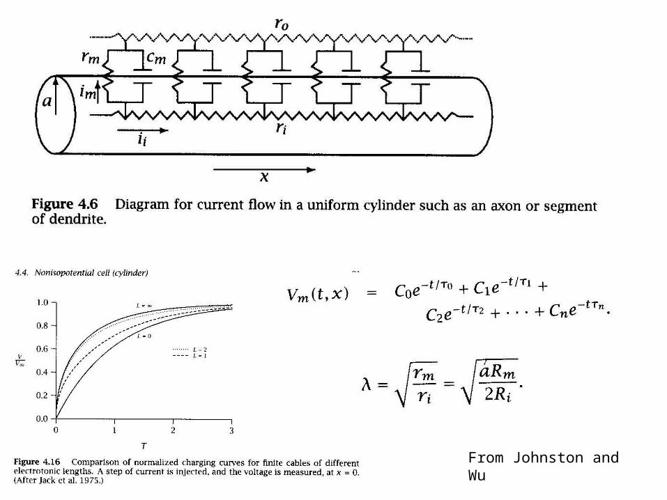
From Johnston and Wu


From Johnston and Wu

From Johnston
and Wu
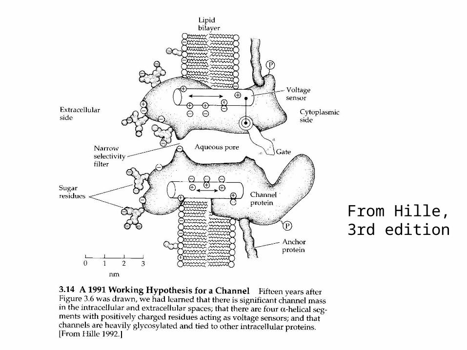
From Hille, 3rd edition


From
DeSchutter and Bower, 1994

Potential Features of Single Cell Processing
•Spatially inhomogenous processing
•signal decay
•signal delay
•shunting
•local amplification
•filtering
•Memory
•Calcium concentration changes integrative properties
•Channel phosphorylation as well
•Time scales: multiple from ms to min to hours/years
•Signal Generation
•plateau potentials
•oscillations
•bursting

1. Create an Accurate Morphological Reconstruction
2. Create an Accurate Passive Model
3. Match active properties with physiological data
Three steps to make a single neuron model

1. Create an Accurate Morphological Reconstruction
2. Create an Accurate Passive Model
3. Match active properties with physiological data
Three steps to make a single neuron model


Rec. A Rec. B Rec. C Rec. D
Length Dendrite 1 m) 1160 1226.3 1378.1 1307.1Surface Area Dendrite 1 (m)2 4829.09 5230.72 4963.62 4344.62Branch Points Dendrite 1 8 8 11 15
Length Dendrite 2 (m) 540.6 508.4 481.3 650.6
Surface Area Dendrite 2 (m) 2 1899.23 1931.47 1057.34 2321.12Branch Points Dendrite 2 4 3 5 6
Length Dendrite 3 (m) 1107.5 1158.4 1133.1 1268.7
Surface Area Dendrite 3 (m) 2 3980.27 4204.36 2641.09 4147.13Branch Points Dendrite 3 7 7 8 9
Length Dendrite 4 (m) 1249.6 1251.9 1242.7 1385
Surface Area Dendrite 4 (m) 2 5352.67 5535.01 3723.33 5007.53Branch Points Dendrite 4 11 9 11 20
Neurolucida (MicroBrightField, Inc.)
Reconstructions
of GP neuron

CVAPP by
Robert Cannon

// Cell morphology file for GENESIS.// Written by cvapp (http://www.neuro.soton.ac.uk/cells/#software).
*absolute*asymmetric*cartesian
// End of cvapp-generated header file.
*origin 0.706 0.756 0
*compt /library/somasoma none 0.706 0.756 0 6.067
*compt /library/dendritep0[1] soma 1.28 9.45 0 1.4p0[2] p0[1] 2.09 12.56 0 1.4p0[3] p0[2] 2.67 15.9 0 1.4p0b1[0] p0[3] 10 21.77 0 1.16p0b1b1[0] p0b1[0] 20.35 22.12 0 0.93p0b1b2[0] p0b1[0] 11.39 29.37 0 0.7p0b2[0] p0[3] -5.93 27.42 0 1.05
p1[1] soma 22.09 -0.35 0 1.63p1b1[0] p1[1] 27.91 9.68 0 1.16p1b2[0] p1[1] 35.35 -7.83 0 0.93

1. Create an Accurate Morphological Reconstruction
2. Create an Accurate Passive Model
3. Match active properties with physiological data
Three steps to make a single neuron model

Task: Set Rm, Cm, and Ri correctly for each compartment
If assumption that parameters are uniform holds, need to fit 3 values.
Strategy: Obtain data from recordings, then optimize Rm, Cm, Ri to fit data.

Message: optimize recordings to get linear (passive) response.
Potential Problems:
• Incomplete Block of Active Properties
• Partial Block of Leak Channels
• Electrode Serial Resistance
• Electrode Shunt

From Major, 1994
Message:
Short current injection pulses have several advantages, obtain such measurements!
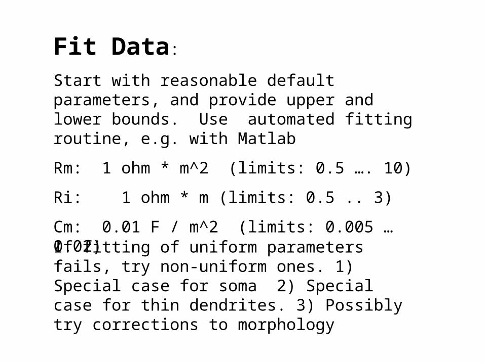
Fit Data:
Start with reasonable default parameters, and provide upper and lower bounds. Use automated fitting routine, e.g. with Matlab
Rm: 1 ohm * m^2 (limits: 0.5 …. 10)
Ri: 1 ohm * m (limits: 0.5 .. 3)
Cm: 0.01 F / m^2 (limits: 0.005 … 0.02)
If fitting of uniform parameters fails, try non-uniform ones. 1) Special case for soma 2) Special case for thin dendrites. 3) Possibly try corrections to morphology
1. Create an Accurate Morphological Reconstruction
2. Create an Accurate Passive Model
3. Match active properties with physiological data
Three steps to make a single neuron model

Tasks:
1) Construct set voltage-gated conductances with correct kinetics.
2) Incorporate intracellular calcium handling
3) Find needed densities of channels in each compartment
4) Add realistic synaptic input conductances

From Destexhe et al., J. Neurosci. (1998). 18:3574-3588

From Destexhe et al., 1998

From Destexhe et al., 1998

From Destexhe et al., 1998
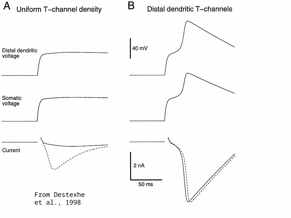
From Destexhe et al., 1998

From Destexhe et al., 1998

From Destexhe et al., 1998

From DeSchutter and Bower, 1994

Calcium Handling
• A Single diffusion shell is a simple solution that works reasonably well.
In this method, a thin (e.g. 0.2 micron) shell of volume below the membrane is taken as a reservoir for calcium with an influx proportional to membrane calcium currents, and an exponential decay to baseline. The baseline concentration is taken from physiological data (e.g. 40 nM).
• More complex solutions include binding to buffers, and intracellular stores. However, it is nearly impossible to get correct kinetic data for these processes.

Finally: Synapses!

From Kondo and Marty, 1998

11-17
Synaptic Potential
Synaptic Currentcapacitive current, resistive current

Potential Shortcomings of simplified synaptic modeling:
•Missing all or none release probability
•Missing minis
•Missing short-term plasticity
•change in release probability, e.g. due to residual Ca
•extrasynaptic receptor activation
•presynaptic receptor activation


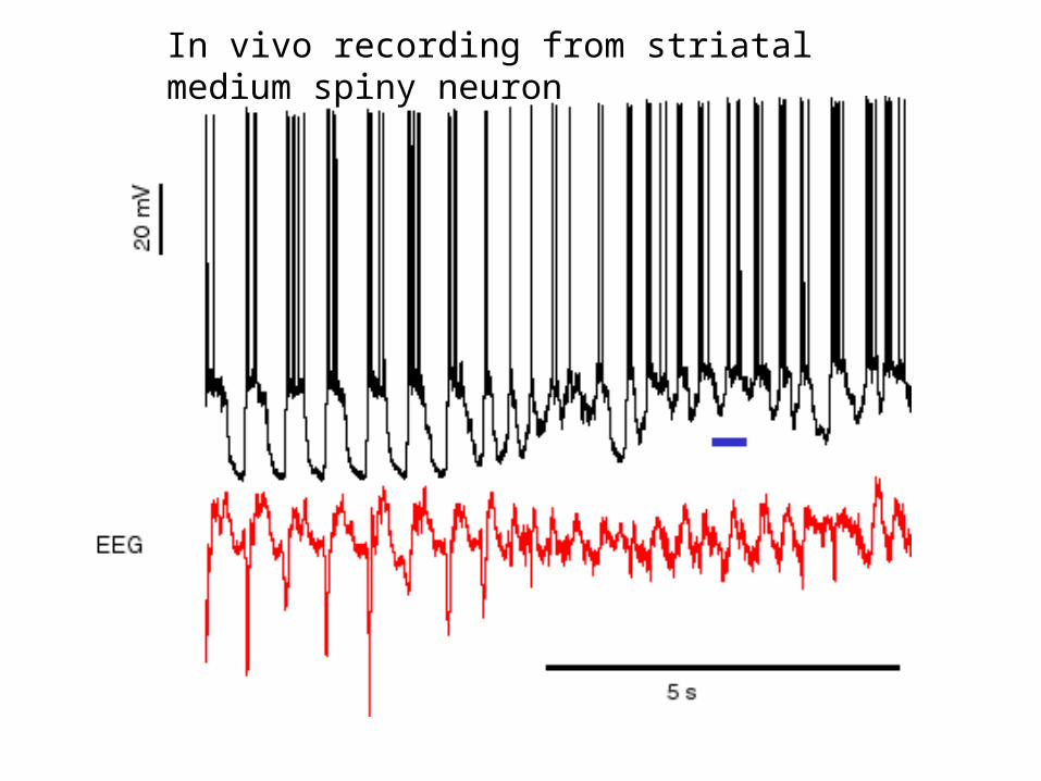
In vivo recording from striatal medium spiny neuron

In vivo recording from striatal medium spiny neuron

The big picture
•Realistic single cell models can be constructed, but it is a lot of work
•Even the best model is still not going to completely replicate biological single cell dynamics
•Each type of neuron is a separate modeling job
•Insight into the processing capabilities of neurons can be gained from realistic single cell modeling
•Experimental predictions can be made and tested
•Insights gained are invaluable for realistic network modeling
•Simplified single cell models are likely required for large network models

Vital References
• Johnston and Wu. Foundations of Cellular Neurophysiology, MIT Press, 1995
• Bertil Hille. Ion Channels of Excitable Membranes. Third Edition. Sinauer, 2001
• Erik De Schutter (editor) Computational Neuroscience: Realistic Modeling for Experimentalists. CRC Press, 2001
• Koch and Segev. Methods in Neuronal Modeling. From Ions to Networks. Second Edition. MIT Press, 1998
• For Beginners in Neuroscience: Kandel, Schwarz, Jessell. Principles of Neural Science, Fourth Edition, McGraw Hill, 2000

A brief primer on how to model complex single cells with Genesis
1. Create morphology file
2. Create channel and compartment prototypes
3. Create main simulation script
4. Create parameter search scheme to tune model
5. Include synapses
6. Enjoy

<genhome>/Scripts/Purkinje/Purk_chansave.g/* Make tabchannels */function make_chan(chan, Ec, Gc, Xp, XAA, XAB, XAC, XAD, XAF, XBA, XBB, \ XBC, XBD, XBF, Yp, YAA, YAB, YAC, YAD, YAF, YBA, YBB, YBC, YBD, YBF \ , Zp, ZAA, ZAB, ZAC, ZAD, ZAF, ZBA, ZBB, ZBC, ZBD, ZBF) str chan int Xp, Yp, Zp float Ec, Gc float XAA, XAB, XAC, XAD, XAF, XBA, XBB, XBC, XBD, XBF float YAA, YAB, YAC, YAD, YAF, YBA, YBB, YBC, YBD, YBF float ZAA, ZAB, ZAC, ZAD, ZAF, ZBA, ZBB, ZBC, ZBD, ZBF if ({exists {chan}}) return end create tabchannel {chan} setfield {chan} Ek {Ec} Gbar {Gc} Ik 0 Gk 0 Xpower {Xp} Ypower {Yp} \ Zpower {Zp} if (Xp > 0) setupalpha {chan} X {XAA} {XAB} {XAC} {XAD} {XAF} {XBA} {XBB} {XBC} \ {XBD} {XBF} -size {tab_xfills+1} -range {tab_xmin} {tab_xmax} end if (Yp > 0) setupalpha {chan} Y {YAA} {YAB} {YAC} {YAD} {YAF} {YBA} {YBB} {YBC} \ {YBD} {YBF} -size {tab_xfills+1} -range {tab_xmin} {tab_xmax} end if (Zp != 0) setupalpha {chan} Z {ZAA} {ZAB} {ZAC} {ZAD} {ZAF} {ZBA} {ZBB} {ZBC} \ {ZBD} {ZBF} -size {tab_xfills+1} -range {tab_xmin} {tab_xmax} endend

/* non-inactivating (muscarinic) type K current, eq#2 ** eq#2: corrected typo in Yamada equation for tau: 20 instead of 40 ** Refs: Yamada (his equations are also for 22C) */ if (!{exists Purk_KM}) create tabchannel Purk_KM setfield Purk_KM Ek {EK} Gbar {GK} Ik 0 Gk 0 Xpower 1 \ Ypower 0 Zpower 0
call Purk_KM TABCREATE X {tab_xdivs} {tab_xmin} {tab_xmax} x = {tab_xmin} dx = ({tab_xmax} - {tab_xmin})/{tab_xdivs}
for (i = 0; i <= ({tab_xdivs}); i = i + 1) y = 0.2/(3.3*({exp {(x + 0.035)/0.02}}) + {exp {-(x + 0.035)/0.02}}) setfield Purk_KM X_A->table[{i}] {y}
y = 1.0/(1.0 + {exp {-(x + 0.035)/0.01}}) setfield Purk_KM X_B->table[{i}] {y} x = x + dx end tau_tweak_tabchan Purk_KM X setfield Purk_KM X_A->calc_mode 0 X_B->calc_mode 0 call Purk_KM TABFILL X {tab_xfills + 1} 0 end call Purk_KM TABSAVE Purk_KM.tab
<genhome>/Scripts/Purkinje/Purk_chansave.g

<genhome>/Scripts/Purkinje/Purk_const.g
* cable parameters */float CM = 0.0164 // *9 relative to passivefloat RMs = 1.000 // /3.7 relative to passive compfloat RMd = 3.0float RA = 2.50/* preset constants */float ELEAK = -0.0800 // Ek value used for the leak conductancefloat EREST_ACT = -0.0680 // Vm value used for the RESET/* concentrations */float CCaO = 2.4000 //external Ca as in normal slice Ringerfloat CCaI = 0.000040 //internal Ca in mM//diameter of Ca_shellsfloat Shell_thick = 0.20e-6float CaTau = 0.00010 // Ca_concen tau
/* Currents: Reversal potentials in V and max conductances S/m^2 *//* Codes: s=soma, m=main dendrite, t=thick dendrite, d=spiny dendrite */float ENa = 0.045float GNaFs = 75000.0float GNaPs = 10.0float ECa = 0.0125*{log {CCaO/CCaI}} // 0.135 Vfloat GCaTs = 5.00float GCaTm = 5.00float GCaTt = 5.00float GCaTd = 5.00float GCaPm = 45.0float GCaPt = 45.0float GCaPd = 45.0float EK = -0.085float GKAs = 150.0float GKAm = 20.0float GKdrs = 6000.0float GKdrm = 600.0float GKMs = 0.400float GKMm = 0.100

if (!({exists Purk_soma}) create compartment Purk_somaend setfield Purk_soma Cm {{CM}*surf} Ra {8.0*{RA}/(dia*{PI})} \Em {ELEAK} initVm {EREST_ACT} Rm {{RMs}/surf} inject 0.0 dia {dia} len {len}
copy Purk_NaF Purk_soma/NaFaddmsg Purk_soma Purk_soma/NaF VOLTAGE Vmaddmsg Purk_soma/NaF Purk_soma CHANNEL Gk Eksetfield Purk_soma/NaF Gbar {{GNaFs}*surf} copy Purk_NaP Purk_soma/NaP addmsg Purk_soma Purk_soma/NaP VOLTAGE Vm addmsg Purk_soma/NaP Purk_soma CHANNEL Gk Ek setfield Purk_soma/NaP Gbar {{GNaPs}*surf} copy Purk_CaT Purk_soma/CaT addmsg Purk_soma Purk_soma/CaT VOLTAGE Vm addmsg Purk_soma/CaT Purk_soma CHANNEL Gk Ek setfield Purk_soma/CaT Gbar {{GCaTs}*surf} copy Purk_KA Purk_soma/KA addmsg Purk_soma Purk_soma/KA VOLTAGE Vm addmsg Purk_soma/KA Purk_soma CHANNEL Gk Ek setfield Purk_soma/KA Gbar {{GKAs}*surf}
copy Purk_Kdr Purk_soma/Kdraddmsg Purk_soma Purk_soma/Kdr VOLTAGE Vmaddmsg Purk_soma/Kdr Purk_soma CHANNEL Gk Eksetfield Purk_soma/Kdr Gbar {{GKdrs}*surf}copy Purk_KM Purk_soma/KMaddmsg Purk_soma Purk_soma/KM VOLTAGE Vmaddmsg Purk_soma/KM Purk_soma CHANNEL Gk Eksetfield Purk_soma/KM Gbar {{GKMs}*surf}
copy Purk_h1 Purk_soma/h1addmsg Purk_soma Purk_soma/h1 VOLTAGE Vmaddmsg Purk_soma/h1 Purk_soma CHANNEL Gk Eksetfield Purk_soma/h1 Gbar {{Ghs}*surf}copy Purk_h2 Purk_soma/h2addmsg Purk_soma Purk_soma/h2 VOLTAGE Vmaddmsg Purk_soma/h2 Purk_soma CHANNEL Gk Eksetfield Purk_soma/h2 Gbar {{Ghs}*surf}create Ca_concen Purk_soma/Ca_poolsetfield Purk_soma/Ca_pool tau {CaTau} \ B {1.0/(2.0*96494*shell_vol)} Ca_base {CCaI} \ thick {Shell_thick} addmsg Purk_soma/CaT Purk_soma/Ca_pool I_Ca Ikcopy GABA2 Purk_soma/basketsetfield Purk_soma/basket gmax {{GB_GABA}*surf}addmsg Purk_soma/basket Purk_soma CHANNEL Gk Ekaddmsg Purk_soma Purk_soma/basket VOLTAGE Vm
<genhome>/Scripts/Purkinje/Purk_cicomp.g

//- include scripts to create the prototypes
include Purk_chanloadinclude Purk_cicompinclude Purk_syn
include info.ginclude bounds.ginclude config.ginclude control.ginclude xgraph.ginclude xcell.g
//- ensure that all elements are made in the library
ce /library
//- make prototypes of channels and synapses
make_Purkinje_chans
<genhome>/Scripts/Purkinje/Purk_cicomp.g
readcell {cellfile} {cellpath}
echo preparing hines solver {getdate}ce {cellpath}create hsolve solve
//- We change to current element solve and then set the fields of the parent//- (solve) to get around a bug in the "." parsing of genesis
ce solve
setfield . \ path "../##[][TYPE=compartment]" \ comptmode 1 \ chanmode {iChanMode} \ calcmode 0
call /Purkinje/solve SETUP
//- Use method to Crank-Nicolson
setmethod 11

include cn_fileout16
outfilev = "data/cn0106c_" @ {simnum} @ "_v_"outfilei = "data/cn0106c_" @ {simnum} @ "_i_"outfilevc = "data/cn0106c_" @ {simnum} @ "_vc_"outfilechan = "data/cn0106c_" @ {simnum} @ "_chan_“
// set up messages to the output files write_voltage soma 0 write_currents_c soma 0 write_chan_activations soma 0 //write_voltage p0b2 0 //write_voltage p0b2b1b2 0 //write_voltage p0b2b1b2 4 write_voltage p0 1 write_voltage p1 1
File Saving System: from DCN simulation by vsteuber
function write_voltage(compt, comptnum)str compt, comptnumstr hinesloc, outfile, outelement, clampstr
outfile = {outfilev @ compt @ comptnum @ "_" @ clampstr @ ".dat"}outelement = "/output/v_" @ {compt} @ {comptnum}
if (!{exists {outelement}}) create asc_file {outelement} echo echo creating output element {outelement} useclock {outelement} 8 hinesloc = {findsolvefield {cellpath} {cellpath}/{compt} Vm} addmsg {cellpath} {outelement} SAVE {hinesloc} end
setfield {outelement} filename {outfile} \ initialize 1 \ leave_open 1 \ append 1
echo echo sending {cellpath}/{compt} Vm to {outfile}.
end

function p_cn6c_sc13(cip,n,fignum1,fignum2,eleak)
addpath('../data')
if (cip < 0.0) ifile = sprintf('cn0106c_%s_chan_soma0_m%spA.dat', num2str(n),num2str(-cip));else ifile = sprintf('cn0106c_%s_chan_soma0_%spA.dat', num2str(n),num2str(cip));endtemp = load(ifile);…
Start of Matlab function to read genesis output.
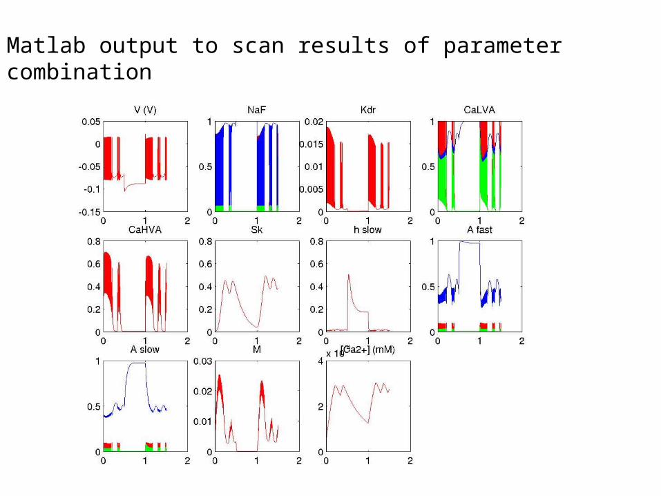
Matlab output to scan results of parameter combination