DEVELOPMENT OF SIMULATION TOOLS ON NANOHUB AS LEARNING MODULES

BY

JULIAN CHINONSO UMEH

A thesis submitted to the Graduate School

in partial fulfillment of the requirements

for the degree of

Master of Science in Chemical Engineering

NEW MEXICO STATE UNIVERSITY

LAS CRUCES, NEW MEXICO

DECEMBER 2019

ii

Copyright © 2019 by JULIAN CHINONSO UMEH B.Eng., M.S

iii

Julian Chinonso Umeh

Candidate

Chemical Engineering

Major This Thesis is approved on behalf of the faculty of New Mexico State University, and it is

acceptable in quality and form for publication:

Approved by the thesis Committee: Dr. Thomas A. Manz

Chairperson Dr. Hongmei Luo

Committee Member Dr. Marat Talipov

Committee Member

iv

ACKNOWLEDGEMENTS

Special thanks to the National Science Foundation (NSF) for funding this project through

CAREER Award DMR-1555376. All tests were performed using the computational clusters

provided by Extreme Science and Engineering Discovery Environment (XSEDE project grant

TG-CTS100027). XSEDE is funded by NSF grant ACI-1548562. I would like to express my

profound gratitude to my advisor Dr. Thomas Manz for his patience and tutelage; I could not

have asked for a better advisor. I would also like to thank members of my committee Dr.

Hongmei Luo and Dr. Marat Talipov, the administrative assistant for the Department of

Chemical & Materials Engineering Carol Dyer, the head of the Department of Chemical &

Materials Engineering Dr. David Rockstraw, as well as members of the nanoHUB support team

for all their help and contributions. Finally, I would like to thank God Almighty, my family, and

friends for their encouragement and support.

v

VITA

2012 Bachelor of Engineering in Chemical Engineering from Enugu State

University of Science and Technology

2017-2019 Research Assistant, Department of Chemical & Materials

Engineering, New Mexico State University

2017-2019 Teaching Assistant, Department of Chemical & Materials

Engineering, New Mexico State University

Field of Study

Major Field: Chemical Engineering

vi

ABSTRACT

DEVELOPMENT OF SIMULATION TOOLS ON NANOHUB AS LEARNING MODULES

BY

JULIAN CHINONSO UMEH

MASTERS OF SCIENCE

NEW MEXICO STATE UNIVERSITY

LAS CRUCES, NEW MEXICO

DECEMBER 2019

DR. THOMAS A. MANZ

Modeling and simulation are both debatably underutilized in teaching and research

institutions. Instructional simulations afford learners the ability to engage in "deep learning"

which enables comprehension as opposed to "surface learning" requiring memorization only and

as such, the importance of simulational learning modules cannot be overemphasized. This project

aims to aid users to better understand the use of the molecular simulation tool RASPA. The

project creates twelve learning modules on nanoHUB, these modules comprise of two integral

parts. The first part is a simulation tool that is a web-based applet linked to RASPA molecular

simulation software on the backend, and is designed to perform and output the results of certain

simulations on nanoHUB.1 The other part of these modules is a PowerPoint presentation

vii

explaining how to use the tool and also how to approach the calculation on RASPA along with

relevant citations.

These modules would engage users and help them understand the functionality of

RASPA. In the end, users should be able to perform certain calculations most especially gas

adsorption and diffusion in metal organic frameworks,2 vapor-liquid equilibrium calculations,

gas-phase properties, liquid-phase properties, metal organic framework surface area and pore

volume etc. using RASPA software. Additionally, it is expected these tools will inspire a new

generation of researchers to see the usefulness of molecular simulation software in the area of

material science.3

Keywords: learning module, nanoHUB, atomistic simulation, RASPA, diffusion, adsorption.

viii

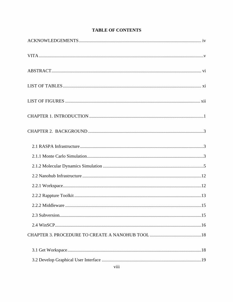
TABLE OF CONTENTS

ACKNOWLEDGEMENTS ........................................................................................................... iv

VITA ................................................................................................................................................v

ABSTRACT ................................................................................................................................... vi

LIST OF TABLES ......................................................................................................................... xi

LIST OF FIGURES ...................................................................................................................... xii

CHAPTER 1. INTRODUCTION ....................................................................................................1

CHAPTER 2. BACKGROUND .....................................................................................................3

2.1 RASPA Infrastructure ............................................................................................................3

2.1.1 Monte Carlo Simulation ......................................................................................................3

2.1.2 Molecular Dynamics Simulation ........................................................................................5

2.2 Nanohub Infrastructure ........................................................................................................12

2.2.1 Workspace.........................................................................................................................12

2.2.2 Rappture Toolkit ...............................................................................................................13

2.2.2 Middleware .......................................................................................................................15

2.3 Subversion............................................................................................................................15

2.4 WinSCP................................................................................................................................16

CHAPTER 3. PROCEDURE TO CREATE A NANOHUB TOOL .............................................18

3.1 Get Workspace .....................................................................................................................18

3.2 Develop Graphical User Interface .......................................................................................19

ix

3.3 Add Lines of Code to Tool Source Code .............................................................................20

3.4 Register Tool on NanoHUB.................................................................................................23

3.6 Edit Middleware File ...........................................................................................................25

3.7 Install Source Code and Approve Tool ................................................................................27

CHAPTER 4. DESCRIPTION OF TOOLS CREATED ..............................................................30

4.1 Gas Diffusion Coefficient in Metal Organic Frameworks ...................................................30

4.2 Gas Adsorption Calculator ...................................................................................................32

4.3 VLE Simulator .....................................................................................................................33

4.4 Mixed Gas Adsorption Calculator .......................................................................................34

4.5 Mixed Gas Diffusion Calculator ..........................................................................................35

4.6 Void Fraction Calculator ......................................................................................................36

4.7 Surface Area Calculator .......................................................................................................37

4.8 Radial Distribution Function Calculator ..............................................................................38

4.9 Adsorption Energy Calculator .............................................................................................39

4.10 NPT Simulator ...................................................................................................................40

4.11 Gibbs Adsorption Simulator ..............................................................................................41

4.12 Henry’s Coefficients Simulator .........................................................................................42

CHAPTER 5. SUMMARY AND OUTLOOK .............................................................................43

5.1 Summary ..............................................................................................................................43

5.2 Outlook ................................................................................................................................45

APPENDIX A ................................................................................................................................46

APPENDIX B ................................................................................................................................57

x

APPENDIX C ................................................................................................................................62

REFERENCES ..............................................................................................................................66

xi

LIST OF TABLES

Table 1. Helpful LINUX commands used to navigate workspace ............................................... 27

xii

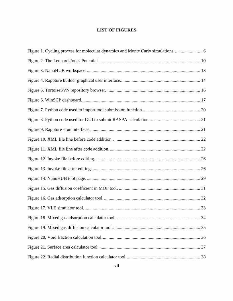
LIST OF FIGURES

Figure 1. Cycling process for molecular dynamics and Monte Carlo simulations. ........................ 6

Figure 2. The Lennard-Jones Potential. ........................................................................................ 10

Figure 3. NanoHUB workspace. ................................................................................................... 13

Figure 4. Rappture builder graphical user interface. ..................................................................... 14

Figure 5. TortoiseSVN repository browser. .................................................................................. 16

Figure 6. WinSCP dashboard. ....................................................................................................... 17

Figure 7. Python code used to import tool submission function................................................... 20

Figure 8. Python code used for GUI to submit RASPA calculation. ............................................ 21

Figure 9. Rappture –run interface. ................................................................................................ 21

Figure 10. XML file line before code addition. ............................................................................ 22

Figure 11. XML file line after code addition. ............................................................................... 22

Figure 12. Invoke file before editing. ........................................................................................... 26

Figure 13. Invoke file after editing. .............................................................................................. 26

Figure 14. NanoHUB tool page. ................................................................................................... 29

Figure 15. Gas diffusion coefficient in MOF tool. ....................................................................... 31

Figure 16. Gas adsorption calculator tool. .................................................................................... 32

Figure 17. VLE simulator tool. ..................................................................................................... 33

Figure 18. Mixed gas adsorption calculator tool. ......................................................................... 34

Figure 19. Mixed gas diffusion calculator tool. ............................................................................ 35

Figure 20. Void fraction calculation tool. ..................................................................................... 36

Figure 21. Surface area calculator tool. ........................................................................................ 37

Figure 22. Radial distribution function calculator tool. ................................................................ 38

xiii

Figure 23. Adsorption energy calculator tool ............................................................................... 39

Figure 24. NPT simulator tool. ..................................................................................................... 40

Figure 25. Gibbs adsorption tool. ................................................................................................. 41

Figure 26. Henry’s coefficient simulator tool. .............................................................................. 42

Figure 27. Sample RASPA input file for adsorption isotherm calculation................................... 46

Figure 28. Sample RASPA input file for diffusion constant calculation. ..................................... 47

Figure 29. Sample RASPA input file for VLE calculation. .......................................................... 48

Figure 30. Sample RASPA input file for mixed gas adsorption calculation. ............................... 49

Figure 31. Sample RASPA input file for mixed gas diffusion calculation. .................................. 50

Figure 32. Sample RASPA input file for void fraction calculation. ............................................. 51

Figure 33. Sample RASPA input file for surface area calculation for MOF. ............................... 51

Figure 34. Sample RASPA input file for radial distribution function calculation........................ 52

Figure 35. Sample RASPA input file for adsorption energy calculation. ..................................... 53

Figure 36. Sample RASPA input file for NPT simulation............................................................ 54

Figure 37. Sample RASPA input file for Gibbs adsorption calculation. ...................................... 55

Figure 38. Sample RASPA input file for Henry’s coefficient simulator. ..................................... 56

Figure 39. Sample skeleton file (main.py) generated by Rappture toolkit. .................................. 57

Figure 40. Sample main.py file for void fraction calculator tool for workspace. ......................... 58

Figure 41. Sample main.py file for void fraction calculator tool for nanoHUB repository. ........ 60

Figure 42. Sample tool.xml file for void fraction calculator tool for workspace. ........................ 62

Figure 43. Sample tool.xml file for void fraction calculator tool for nanoHUB repository. ........ 64

1

CHAPTER 1. INTRODUCTION

Simulation is the production of a computer model of something especially for the purpose

of study. It is a very powerful and important tool that provides a way to test different hypotheses,

try different experimental conditions and parameters, alternative concepts and designs without

having to carry out experiment on real systems which may be too expensive or time-consuming.

It is thus ingenious to utilize it in areas of materials research to study adsorption and diffusion of

gas molecules through nanoporous materials such as metal organic frameworks.

This project involves the development of twelve simulation modules on nanoHUB.

NanoHUB is an online platform for science and engineering originally funded by the National

Science Foundation (NSF). NanoHUB comprises of simulation tools and resources developed

and contributed by members of the community. It promotes the advancement of nanoscience and

nanotechnology and professional collaboration. NanoHUB is a product of the Network for

Computational Nanotechnology (NCN) which aids research efforts in the area of nanoscience

and nanotechnology. NanoHUB can be accessed through the web portal nanohub.org. It contains

over 500 simulation tools, about 5500 resources. It has over 2200 citations in scientific literature

with over 1.4 million yearly users worldwide. It allows users to run simulations on their web

browser as applets but these simulations are powered by sophisticated supercomputers. These

simulations run transparently in a scientific cloud that uses Purdue University and national grid

resources.

The primary objective of this project is to create twelve learning modules on nanoHUB

involving simulation tools and PowerPoint presentations that will:

2

1. Demonstrate basic inputs, outputs, and methods for classical molecular dynamics and

Monte Carlo simulations using RASPA software.

2. Foster the interest of new students and researchers to study diffusion constants,

adsorption isotherms, vapor-liquid equilibrium, gas-phase and liquid-phase properties by

educating them on the use of RASPA to perform these calculations.

3

CHAPTER 2. BACKGROUND

2.1 RASPA Infrastructure

RASPA is a molecular simulation software used for simulating adsorption and diffusion

of molecules in flexible nanoporous materials such as carbon nanotubes, metal organic

frameworks, and zeolites. It uses the most recent cutting edge algorithms to perform molecular

dynamics (MD) and Monte Carlo (MC) calculations in various ensembles.4 Monte Carlo and

molecular dynamics methods can be combined to form more advanced simulations for

specialized applications such as adsorption on a swelling material,5 protein studies,6 lipids

studies,7 etc.

2.1.1 Monte Carlo Simulation

The Monte Carlo method is an algorithm used to measure the value of an unknown

quantity using inferential statistics. It involves the repetition of random sampling to obtain a

numerical value and solve a problem that might be deterministic in principle.4 Monte Carlo relies

on equilibrium statistical mechanics, it generates the state of the system according to appropriate

Boltzmann probabilities. MC methods can be applied to a variety of molecular studies such as

adsorption calculations,8 vapor-liquid equilibrium calculations,9 chemical reactions,10 etc.

Each Monte Carlo move follows these steps. It first randomly selects the type of move to

perform (i.e., translation, rotation, reinsertion, etc.). Next it randomly picks a molecule on which

to perform the move (unless it’s a volume change move). It randomly decides how to perform

4

that move on that molecule (e.g., the magnitude of translation or the degree of rotation, etc.). It

performs the move and then it calculates the Boltzmann factor for that system configuration

(move). The Boltzmann factor is given by exp(-∆E/(kT)) and it expresses the probability of a

state of energy relative to another state of energy. ∆E is the change in energy of the system, k is

the Boltzmann constant, and T is the absolute temperature of the system. In this case, ∆E would

be the system energy after the move minus the system energy of the prior configuration. Finally,

it decides whether to accept or reject the configuration.11, 12 It achieves this by first generating a

random number from a uniform distribution between 0 and 1, and the value of the Boltzmann

factor calculated is compared to this number. If the Boltzmann factor is less than the random

number, the move is rejected. If it the Boltzmann factor is greater than the number generated, the

move is accepted. If the move is rejected, the new configuration retains the configuration of the

previous move.

Some common Monte Carlo moves made by RASPA include:

Translation: This move stochastically displaces (translates) a random molecule in the

allowed direction to a certain distance from its original position.

Rotation: This move randomly selects a molecule and rotates it about its axis.

Swap: This is an insertion or deletion move, it randomly decides whether to insert or

delete a molecule from the system. The probability of insertion and deletion is 50%.

Reinsertion: This move randomly selects a molecule, remove it from its position and

reinserts the molecules into a different position in the system.

5

In RASPA, every Monte Carlo simulation is first initialized at the beginning of the

simulation. The initialization cycle equilibrate the position of molecules in the system.11 Data is

collected during production cycle.

2.1.2 Molecular Dynamics Simulation

The molecular dynamics (MD) algorithm calculates the time-dependent behavior of

molecular systems like their atomic positions and velocities. The concept of MD is simple: it

takes advantage of the fact that Newton’s equation of motion links forces to acceleration.13 The

trajectories of atoms and molecules are calculated numerically by solving Newton’s equation for

interacting particles. The forces of interaction and the potential energy of the atoms and

molecules are calculated using the interatomic potentials or force fields. The simulation is started

with a configuration of the atoms and the force on each atom is computed. Then, the force is

turned into acceleration. Using a numerical time step algorithm the acceleration is combined with

information on the current and previous atomic positions and velocities to predict the position of

each atom a small time interval later (time step).13

In RASPA, just like with Monte Carlo (MC) simulations, molecular dynamics (MD)

simulations are first initialized at the beginning of the simulation (initialization cycle). As stated

earlier, initialization cycles use Monte Carlo moves to rapidly equilibrate the position of

molecules in the system.11 Next, the system is even further equilibrated during the equilibration

cycles. Equilibration cycles use MD moves to equilibrate the velocities in the systems.11 Figure 1

6

depicts the cycling process in a typical MC and MD simulation. It should be noted that Monte

Carlo simulations that use a single probe particle test insertion (not a thermodynamic ensemble)

do not need initialization cycles.

Figure 1. Cycling process for molecular dynamics and Monte Carlo simulations.

Common thermodynamic ensembles used for MD include:

Microcanonical ensemble (NVE) – This statistical ensemble holds the number of

particles N, the volume V, and the energy E constant during the course of the simulation

Canonical ensemble (NVT) – This ensemble holds the number of particles N, the

volume V, and the average temperature T constant.

Initialization

Cycles

Production

Cycles

Initialization

Cycles

Equilibration

Cycles

Production

Cycles

Monte Carlo MD Cycles

CcCycles

7

Isobaric-Isothermal ensemble (NPT) – With this ensemble, the number of particles N,

the average pressure P, and the average temperature T are held constant.

Isoenthalpic-Isobaric ensemble (NPH) – Here the number of particles N, the average

pressure P, and the enthalpy are held constant.

Some simulations performed using the molecular dynamics algorithm include: diffusion

coefficients (both self-diffusion and collective diffusion),14 molecular interaction,15 material

characteristics,16 chemical reactions,10 protein folding,17 etc. In this project, MD calculations for

diffusion constant is limited to self-diffusivity. Self-diffusion is the diffusive motion of a single

particle.18 It is mathematically given as:

N

2

i ix

s

i 1

1 dlim r t r 0

2dN dtD

(1)

where Nis number of molecules of component α, d is the number of spatial dimensions, ir

is

the center of mass of molecule i of component α, and t is time. In a molecular dynamics

simulation, it is computed by taking the slope of the mean squared displacement (MSD) at long

times. MSD accuracy rapidly decreases over increasing times therefore the slope is only fitted to

a few points in the middle where the MSD is linear.

On the other hand, collective diffusivity (also known as transport diffusivity) describes

transport of mass and the decay of density fluctuations in the system.18 It is the proportionality

constant relating a macroscopic flux to a spatial concentration gradient in Fick’s law,19 and is

given by the equation:

8

2

N

i ix

i 1

T dlim r t r 0

2dN dD

t

(2)

22T

Nln f

ln c N N

(3)

where is the thermodynamic factor, f is fugacity, c is the concentration (adsorbate loading in

the framework) which can be calculated using the adsorption isotherm, and T is absolute

temperature.

2.1.3 Forcefields

In a molecular simulation, forcefields are parameters used to calculate the potential

energy between atoms and molecules.20-22 The basic functional form of potential energy in

molecular mechanics involves the bonded and non-bonded interactions.23 This can be expressed

mathematically as:

E = Ebonded + Enonbonded (5)

Ebonded = ER + Eθ + Eφ + Eω (6)

Enonbonded = Evdw + Eel (7)

where ER is the bond stretch interaction, Eθ the bond angle bending, Eφ is the dihedral angle

torsion, Eω is the inversion term, Evdw is the van der Waal energy and Eel the electrostatic

energy.23 The bonded terms are used to specify interactions between atoms linked by a covalent

bond.24

9

The non-bonded interactions on the other hand consist of the electrostatic term and the

van der Waals interaction. The electrostatic term uses Coulomb’s law to account for the force felt

as a result of the particle charge.25 The van der Waals term includes a wide range of

intermolecular interactions all summed up, these include: exchange-repulsion, polarizabilities,

and dispersion. These interactions are distant dependent as they only occur when the molecules

are within a short distance. The exchange-repulsion energy is the repulsive energy felt as a result

of Pauli exclusion principle which prevents the collapse of molecules.26 Polarizability accounts

for the ability of molecules to form dipoles, it is an attractive interaction between a permanent

multipole on one molecule with an induced multipole on another.27-32 The dispersion term

(London dispersion) specifies the attraction interaction between nonpolar molecules which

occurs as a result of the interaction of instantaneous multipoles.33-38

The non-bonded parameters are the most computationally expensive parameters to

calculate, hence the popular choice to limit interactions to pairwise energies. This has also

prompted the use of the Lennard-Jones potential for the specification of the van der Waal

interactions. The Lennard-Jones potential is given by the equation:

12 6

LJV 4r r

(8)

ε is the depth of the potential well, σ is the finite distance at which the inter-particle potential is

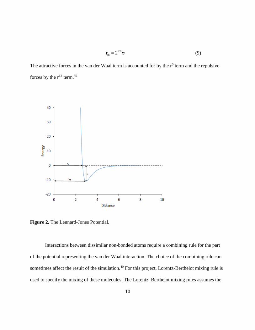
zero, and r is the distance between the molecules. Figure 2 shows a typical potential energy

curve for two interacting molecules. rm is the is the distance at which the potential reaches its

minimum. It is related to σ by:

10

1/6

mr 2 (9)

The attractive forces in the van der Waal term is accounted for by the r6 term and the repulsive

forces by the r12 term.39

Figure 2. The Lennard-Jones Potential.

Interactions between dissimilar non-bonded atoms require a combining rule for the part

of the potential representing the van der Waal interaction. The choice of the combining rule can

sometimes affect the result of the simulation.40 For this project, Lorentz-Berthelot mixing rule is

used to specify the mixing of these molecules. The Lorentz–Berthelot mixing rules assumes the

11

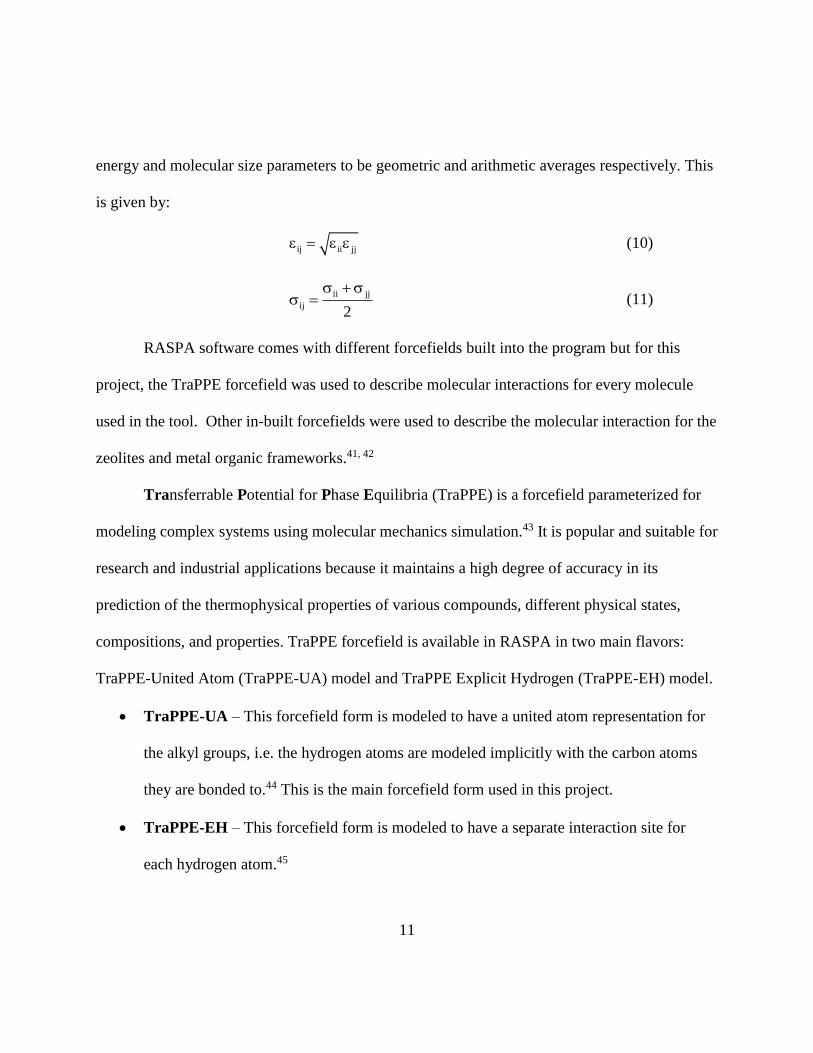
energy and molecular size parameters to be geometric and arithmetic averages respectively. This

is given by:

ij ii jj (10)

ii jj

ij2

(11)

RASPA software comes with different forcefields built into the program but for this

project, the TraPPE forcefield was used to describe molecular interactions for every molecule

used in the tool. Other in-built forcefields were used to describe the molecular interaction for the

zeolites and metal organic frameworks.41, 42

Transferrable Potential for Phase Equilibria (TraPPE) is a forcefield parameterized for

modeling complex systems using molecular mechanics simulation.43 It is popular and suitable for

research and industrial applications because it maintains a high degree of accuracy in its

prediction of the thermophysical properties of various compounds, different physical states,

compositions, and properties. TraPPE forcefield is available in RASPA in two main flavors:

TraPPE-United Atom (TraPPE-UA) model and TraPPE Explicit Hydrogen (TraPPE-EH) model.

TraPPE-UA – This forcefield form is modeled to have a united atom representation for

the alkyl groups, i.e. the hydrogen atoms are modeled implicitly with the carbon atoms

they are bonded to.44 This is the main forcefield form used in this project.

TraPPE-EH – This forcefield form is modeled to have a separate interaction site for

each hydrogen atom.45

12

2.2 Nanohub Infrastructure

Some nanoHUB infrastructure used in the development of the tools in this project

include: workspace, Rappture toolkit, middleware, and repository. Workspace is used to deploy

Rappture toolkit, Rappture toolkit is used to develop the graphical user interface (GUI), and

middleware is used to tie-in the GUI to RASPA.

2.2.1 Workspace

A workspace is an in-browser Linux desktop that provides access to computational

resources on NCN’s network. Workspace provides the platform on which Rappture toolkit used

for tool development is be deployed. The workspace can be used to develop (code), test, compile

and debug new simulation tools before they are ready to be deployed on nanohub46. Figure 3

depicts nanoHUB workspace.

13

Figure 3. NanoHUB workspace.

2.2.2 Rappture Toolkit

Rappture is an acronym for Rapid application infrastructure. As its name implies, it is a

tool to develop simulation tools on nanoHUB. It makes tool development a quick and easy

process by allowing users to drag and drop functionality from the “Object Type” as shown in

Figure 4 to the “Tool Interface” input and output. It generates two skeleton files. The first file

generated “tool.xml” is an extensible markup language (XML) file that contains all the input and

output selected and predefined in the Rappture builder. This file automatically generates a

graphical user interface (GUI)47. Developing a GUI is the first half of building a simulation tool,

the other half is writing code within the simulator to access inputs, run calculations and spit out

14

the results. For this Rappture has a variety of programming languages it can execute, these

include: Python, Fortran 77, C/C++, Octave, Java, Perl, Tcl, R, Ruby, etc. The other file

generated by Rappture builder is the main program in the simulator, this file contains the set of

command that retrieve the input data from the GUI, perform the calculations and finally send

back the result to the GUI. This file is named “main.ext”; where “ext” is the extension of the file

based on the chosen programming language (e.g., “main.py” for Python).

Figure 4. Rappture builder graphical user interface.

15

2.2.2 Middleware

Middleware is a webserver that dynamically relays incoming virtual network computing

connections to an execution host on which an application session is running. It is basically a

software that provides services to other software applications beyond those available from the

operating system, it is the software layer that lies between the operating system and the

applications on each side of a distributed computing system in a network. It links the web applet

(graphical user interface) and RASPA molecular simulation software using a set of commands in

a file named “invoke”.

2.3 Subversion

Subversion also known by its abbreviation SVN is a version control software developed by

Apache Software Foundation. Subversion is a centralized system for sharing information.

Software developers working on a project use subversion to maintain current and previous

versions of their files such as codes, web pages, and documentation. SVN tracks changes made

to each file and can revert to a previous version if they so desire, because subversion stores every

change ever made to the file. At its core, it is a repository which is basically a bank for data

storage. The repository stores information in the form of a file system tree48. Subversion works

on Win 32, MacOS X but is mostly used with Unix/Linux operating systems; instead for

Windows operating system, TortoiseSVN is used. TortoiseSVN depicted in Figure 5 is a

subversion client implemented as a Windows shell extension which makes it easy to use as it

16

does not require a subversion command line client49. For this project, a PC with Windows

operating system was used thus TortoiseSVN was utilized as the version control software.

Figure 5. TortoiseSVN repository browser.

2.4 WinSCP

WinSCP stands for windows secure copy, it is an open source Secure Shell File Transfer

Protocol (SFTP) client for Windows. It is used to transfer files securely between a local

computer and a remote computer. Other basic tasks performed by WinSCP include: navigating a

computer, uploading files, downloading files, synchronizing local and remote directory, editing

17

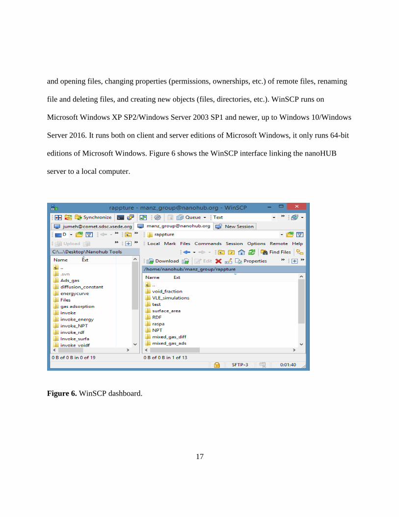
and opening files, changing properties (permissions, ownerships, etc.) of remote files, renaming

file and deleting files, and creating new objects (files, directories, etc.). WinSCP runs on

Microsoft Windows XP SP2/Windows Server 2003 SP1 and newer, up to Windows 10/Windows

Server 2016. It runs both on client and server editions of Microsoft Windows, it only runs 64-bit

editions of Microsoft Windows. Figure 6 shows the WinSCP interface linking the nanoHUB

server to a local computer.

Figure 6. WinSCP dashboard.

18

CHAPTER 3. PROCEDURE TO CREATE A NANOHUB TOOL

The procedures for creating a simulation tool on nanoHUB would vary slightly

depending on the programming language used in writing the code and the tool function. Listed

below are the steps taken to create the simulation tools for this project based on Python:

1. Get approved for workspace and install RASPA.

2. Develop graphical user interface (GUI).

3. Add lines of code to source code.

4. Register tool on nanoHUB.

5. Upload code to the repository.

6. Edit middleware invoke file and make executable.

7. Install source code and approve tool for publishing.

3.1 Get Workspace

To create a tool on nanoHUB, one has to first create an account and become a member of

the community. The next step is to get approved for workspace and install RASPA. A support

ticket has to be created to get approved for workspace. To create a ticket, the user would click on

“SUPPORT” found on the upper right-hand corner of the screen on the homepage and then click

on “Tickets”. In the ticket, the user would enter the name, description, use, and target audience

of the tool to be developed. A member of the support team would review and approve the

request. Similarly, to get RASPA installed, a separate ticket is created. This ticket contains a

19

description of the program to be installed (RASPA), as well as a link to the source code on

GitHub. This process only has to be done once for any account created on nanoHUB.

3.2 Develop Graphical User Interface

After the installation of RASPA and the approval of workspace, the next step is to

develop a graphical user interface (GUI) using Rappture toolkit which comes preinstalled in

workspace. To launch workspace, the user navigates to the dashboard by clicking on “Logged

in” on the right-hand corner of the homepage and then clicks on “Dashboard” from the drop-

down list. On the dashboard click “Workspace” which is on the lower-left corner of the

dashboard under “MY TOOLS”. After the workspace is opened, the user would then launch

Rappture toolkit by using the command into the UNIX shell “rappture –builder”, refer to Figure

4 to see Rappture builder interface. Using Rappture toolkit, a GUI could be developed. This is

done by adding various functionalities to the GUI by simply dragging object types over to tool

interface to populate the input and output section. Examples of some object types include:

Boolean, Label, String, Curve, Number, etc. After adding these functions to the input and output,

the next step involves the description of these functions by clicking on each of them and filling

the required information. The object type selected for the input and output both depend on the

tool being created and the design philosophy adopted. Finally, the “Tool” option under tool

interface needs to be filled. Here the tool title is filled in, the tool description is given, and the

20

programming language of choice chosen. Once all that is done and saved, Rappture develops two

files, a skeleton Python file named “main.py” and an XML file named “tool.xml”.

3.3 Add Lines of Code to Tool Source Code

At this stage of the project, several lines of codes are written to the skeleton file

“main.py” in Python programming language. The code written varies between developers; it

depends on the design philosophy adopted by the tool developer. However, for this project the

lines of code added to this file do the following;

1. Create an input file for RASPA simulation using data selected or inputted into GUI.

2. Submit calculation and update the user on the progress of the simulation.

3. Retrieve results of calculation performed and output result into GUI.

To open the skeleton file (main.py), the developer would have to install and log into their

nanoHUB account on WinSCP to ease the process of writing and editing the source code file.

The design philosophy adopted for this project involves writing scripts that open RASPA input

file named “simulation.input” and appends lines of instructions for the simulation based on user

input. For the GUI to run the RASPA simulation, the line of code written is shown in Figure 7

and Figure 8.

Figure 7. Python code used to import tool submission function.

21

Figure 8. Python code used for GUI to submit RASPA calculation.

After the addition of lines of code to the file, the tool can be tested and debugged. Similar

to the command used to open Rappture interface for building the tool, the command typed into

the workspace command prompt to test run the tool is “rappture –run”; this opens the tool GUI

and allows the developer to use (test) the tool. Figure 9 shows the GUI for a typical tool

developed using Rappture.

Figure 9. Rappture –run interface.

22

Once the tool is tested and confirmed to be working on workspace, additional lines of

code must be added to the source code and the XML file before being uploaded to the repository

as shown below in Figure 10 and Figure 11. In the XML file, this code word (@tool) is added in

the “<tool>” section under “<command>”. This is added to ensure that the tool works after it is

installed on the nanoHUB. Similarly, some lines of codes were edited in the “main.py” file and

changes were made to account for the design philosophy adopted. This is important because

without having the code written in that format, the tool would not run. Sample “main.py” and

“tool.xml” files from the same tool, (one for workspace and the other for repository) can be

found in Appendix B and Appendix C respectively with relevant changes highlighted to show the

difference.

Figure 10. XML file line before code addition.

Figure 11. XML file line after code addition.

23

3.4 Register Tool on NanoHUB

Once the tool is ready to be installed, the developer would have to first register the tool

and create a description page. To achieve this, the developer would have to click on the “Tools”

option in “RESOURCES” menu on the upper right corner on the homepage and then click “Start

a new Tool”. There the user can specify the desired tool name, title, repository host, access

options, publishing option, etc. Subversion should be selected as the repository host by checking

the radio button “Host subversion repository on HUB”. Right after the tool is registered on

nanoHUB, it automatically creates a repository for the tool. A page describing the tool can then

be created by clicking “Edit page description”, this page would usually contain the summary or

description of the tool, other details like citations, references, sponsors, screenshots, authors,

supporting documentation, tags, etc. are also included in the description page. After the tool is

registered and the description page created, the source code can then be uploaded to the

repository and installed for additional testing and debugging.

3.5 Upload Source Code to Repository

Before the source code can be uploaded on nanoHUB, TortoiseSVN first needs to be

installed on local computer for PC running on Windows operating system, or Subversion (SVN)

for Linux operating systems. SVN and TortoiseSVN are free and easy to install. To upload the

source code, a local repository must be created on the developer’s local computer, this is simply

a folder where files would be moved to from nanoHUB workspace. Files can be moved between

workspace and local computer using WinSCP. When the source code is in the designated folder,

24

that folder can be made to become the local repository for that tool and the source code can be

uploaded to the repository on nanoHUB. From the local repository, changes can be made to the

source code and updated so it would reflect on nanoHUB repository. As stated earlier, nanoHUB

automatically creates a repository for a tool when it is registered. This repository contains three

main folders named branches, tags, and trunks. The trunk folder is the main folder where the

source code is uploaded, it contains the following subfolders: bin, data, doc, examples,

middleware, rappture and src. The subfolder “rappture” is where the source code would be

uploaded. To upload the source code, navigate to the repository on the local computer where

source code is saved, then right-click and scroll down to “TortoiseSVN” option, then click on

“import”. Next, enter the URL path of the repository on nanoHUB. This can be obtained from

the wiki page found on the tool page, click on the hyperlink “GettingStarted” to find this

information. It should be noted that the URL path follows this convention:

https://nanohub.org/tools/toolname/svn/trunk/rappture

Where “toolname” is the name assigned to the tool when it was registered on nanoHUB. For

example, if the tool name is “chemsim”, the URL would be:

https://nanohub.org/tools/chemsim/svn/trunk/rappture

The last part of the URL path (/rappture) is not included in the URL on the wiki page but should

be included in the URL used in TortoiseSVN to move the source code to that folder.

25

3.6 Edit Middleware File

In the tool repository, there is a folder named middleware folder containing a file

“invoke” which connects the graphical user interface (GUI) to the RASPA software using

Python. This file is an executable file containing a few lines of code written in Linux shell

scripts. When nanoHUB generates the repository for the tool, it also writes the Linux shell

scripts for the middleware file (invoke) but the scripts are written as comments and the file made

nonexecutable. Hence the need to go into the file, uncomment and edit the script to suit the

programs used in developing and running the tool. To edit the file, a new folder is created and

from the folder, right-click and select “SVN Checkout…” then enter the URL path for the

middleware folder; this can be obtained from the repository browser. To navigate the repository

browser, right-click and select “TortoiseSVN” and then click “Repo-browser”. After the

middleware file has been checked out to the local computer repository, it can be edited and

recommitted to the repository by right-clicking and selecting “SVN commit…”. To make the file

executable, open the repository browser and navigate to the middleware folder, right-click on the

file (invoke) and select “show properties”, click on “New” and select “Executable”, check the

box “Executable” and then click “OK”. Figure 12 and Figure 13 are for the same tool (Radial

Distribution Function Calculator) with the alias “rdf” assigned to it during the registration of the

tool.

26

Figure 12. Invoke file before editing.

Figure 13. Invoke file after editing.

Table 1 shows some Linux commands used to navigate workspace, this is important

because for every tool developed, the source code is put in a new directory and as such, a new

folder is created every time.

27

Table 1. Helpful LINUX commands used to navigate workspace

Command Function

mkdir Creates a new directory/folder

ls Lists all existing files in a folder

nano Used to edit a file

pwd Shows current directory

cd Change directory

3.7 Install Source Code and Approve Tool

After the source code has been uploaded and the middleware file edited, the tool is ready

to be installed, tested and published. Clicking the hyperlink “I’ve committed new code. Please

install the latest version for testing and approval” on nanoHUB tool page depicted in Figure 14

alerts support and lets them know that the tool is ready for installation. It could take up to 72

hours for support to have the code installed, but it usually takes less than 12 hours. After the tool

is installed, tests should be performed to ensure it runs well. If there are issues with the tool that

the developer is unsure how to fix, the developer should reach out to support and ask for their

help by creating a ticket. If there are changes to the source code, the changes should be made to

the source code on the developer’s local repository on their PC and the source code should be

28

recommitted to the repository and the new code installed. This cycle should be repeated until the

developer is satisfied with the performance of the tool.

29

Fig

ure

14. N

anoH

UB

to

ol

pag

e.

30

CHAPTER 4. DESCRIPTION OF TOOLS CREATED

Below is list of the tools created and their description:

1. Gas Diffusion Coefficient in Metal Organic Frameworks

2. Gas Adsorption Calculator

3. VLE Simulator

4. Mixed Gas Adsorption Calculator

5. Mixed Gas Diffusion Calculator

6. Void Fraction Calculator

7. Surface Area Calculator

8. Radial Distribution Function Calculator

9. Adsorption Energy Calculator

10. NPT Simulator

11. Gibbs Adsorption Simulator

12. Henry’s coefficients simulator

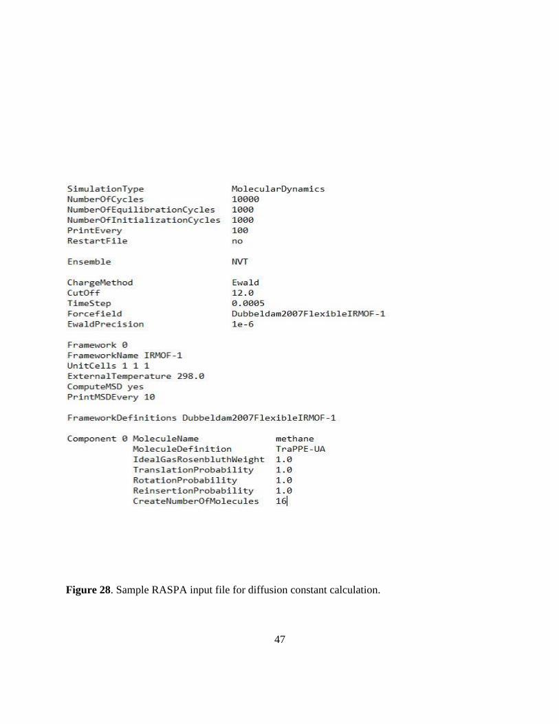
4.1 Gas Diffusion Coefficient in Metal Organic Frameworks

This tool calculates the self-diffusion constant of gas molecules through a metal organic

framework (MOF) using the molecular algorithm with the NVT ensemble. The gases used for

the simulation includes: helium, hydrogen, nitrogen, methane, and carbon dioxide. The user

selects the gas and metal-organic framework from drop lists. The MOFs used for the tool are

31

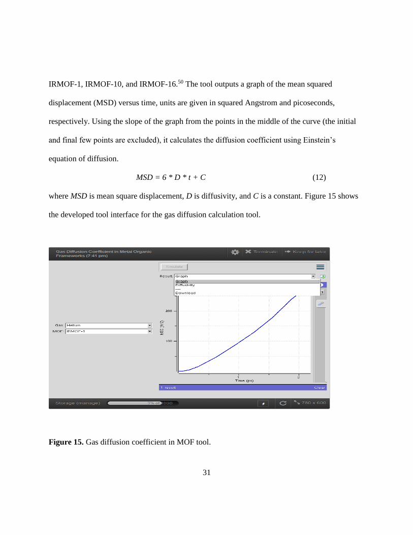
IRMOF-1, IRMOF-10, and IRMOF-16.50 The tool outputs a graph of the mean squared

displacement (MSD) versus time, units are given in squared Angstrom and picoseconds,

respectively. Using the slope of the graph from the points in the middle of the curve (the initial

and final few points are excluded), it calculates the diffusion coefficient using Einstein’s

equation of diffusion.

MSD = 6 * D * t + C (12)

where MSD is mean square displacement, D is diffusivity, and C is a constant. Figure 15 shows

the developed tool interface for the gas diffusion calculation tool.

Figure 15. Gas diffusion coefficient in MOF tool.

32

4.2 Gas Adsorption Calculator

This tool calculates the average absolute and excess adsorption of gas molecules onto a

metal organic framework using Monte Carlo algorithm with the grand canonical ensemble

(μVT). The gases used for the simulation include: helium, hydrogen, nitrogen, oxygen, methane,

and carbon dioxide. The frameworks used for the tool are IRMOF-1, IRMOF-10, and IRMOF-

16.51, 52 The user can select from drop lists, the type of gas as well as MOF for the simulation. It

also allows the user to enter the temperature and pressure for the simulation. The tool outputs the

average absolute adsorption and the average excess adsorption as shown in Figure 16.

Figure 16. Gas adsorption calculator tool.

33

4.3 VLE Simulator

VLE stands for vapor liquid equilibrium. Like the name implies, this tool simulates the

vapor-liquid equilibrium of gas molecules using Monte Carlo algorithm with Gibbs ensemble.53

The molecule choices are the first five alkanes: methane, ethane, propane, butane and pentane.

The tool requires the user to select the molecule, and enter the simulation temperature, then it

outputs the equilibrium pressure, gas density and liquid density as shown in Figure 17. The tool

has a limitation, it gets less accurate farther away from the boiling point. This is because the

simulation is setup with only 1000 cycles and does not allow enough time for the simulation to

equilibrate the liquid and the vapor phase. Therefore, it is suggested that the simulation

temperature is kept between - 50 Kelvin and +50 Kelvin from the boiling temperature at

atmospheric pressure.

Figure 17. VLE simulator tool.

34

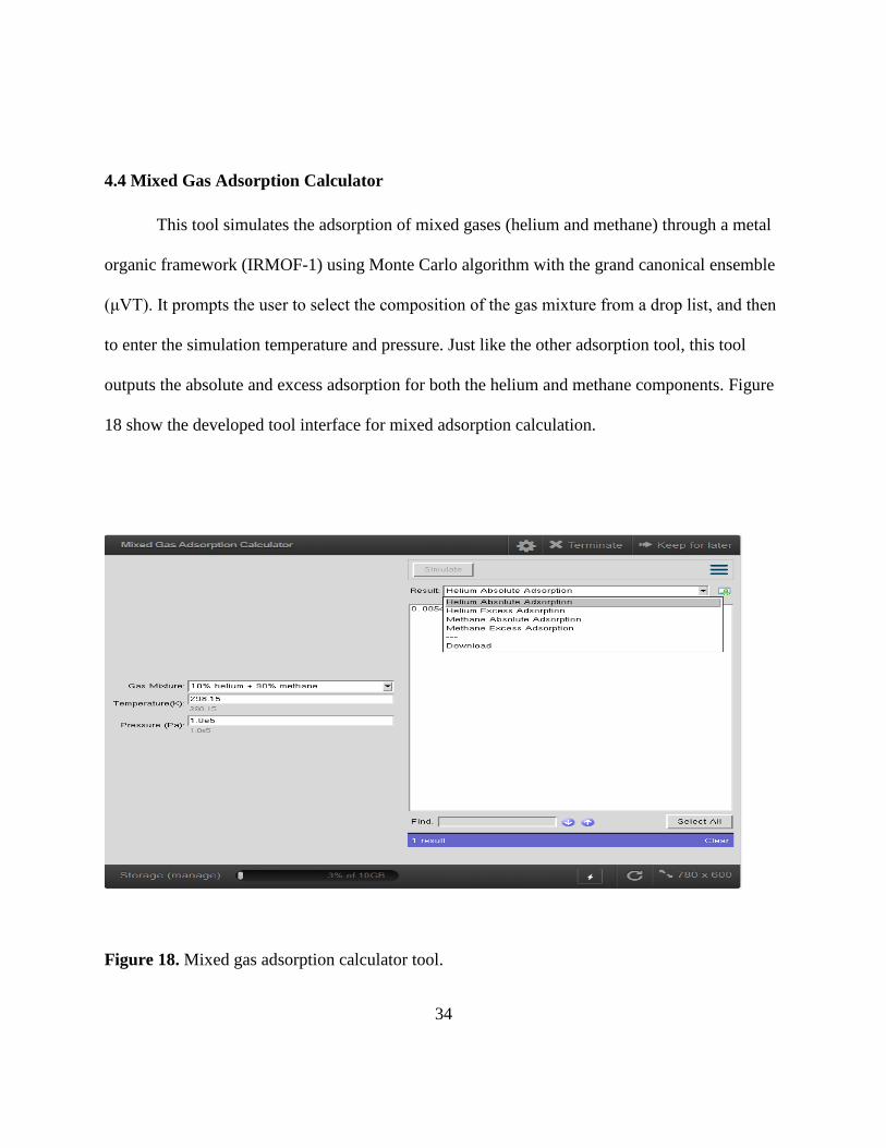
4.4 Mixed Gas Adsorption Calculator

This tool simulates the adsorption of mixed gases (helium and methane) through a metal

organic framework (IRMOF-1) using Monte Carlo algorithm with the grand canonical ensemble

(μVT). It prompts the user to select the composition of the gas mixture from a drop list, and then

to enter the simulation temperature and pressure. Just like the other adsorption tool, this tool

outputs the absolute and excess adsorption for both the helium and methane components. Figure

18 show the developed tool interface for mixed adsorption calculation.

Figure 18. Mixed gas adsorption calculator tool.

35

4.5 Mixed Gas Diffusion Calculator

This tool simulates the self-diffusion of gas mixtures through a metal organic framework

(MOF) using the molecular dynamics algorithm with the NVT ensemble. The gases used in this

tool are helium and methane, and the MOF used is IRMOF-1. The tool prompts the user to select

the composition of the gas mixture from a drop list, and then to enter the simulation temperature.

The tool outputs a graph of the mean squared displacement (MSD) versus time for both helium

and methane, and using the slope of the curve from the points in the middle of the curve (the

initial and final few points are excluded), it calculates the self-diffusivity and outputs the value.

Figure 19 depicts the developed tool interface for mixed gas diffusion calculation.

Figure 19. Mixed gas diffusion calculator tool.

36

4.6 Void Fraction Calculator

The void fraction calculator tool simulates the pore volume of nanoporous materials. The

nanoporous materials being calculated include both metal organic frameworks and zeolites such

as: IRMOF-1, IRMOF-10, IRMOF-16, ITQ-1, ITQ-3, ITQ-7, ITQ-12, ITQ-29, KFI, LTA4A,

and LTA5A. The tool is very simplistic in design: it requires the user to select (from a drop list)

the material for which they want to calculate the pore volume. Using Monte Carlo algorithm to

perform random particle insertion (Widom insertion) thereby probing the material, the tool

calculates the void fraction of the material. Figure 20 shows the developed tool interface for void

fraction calculation.

Figure 20. Void fraction calculation tool.

37

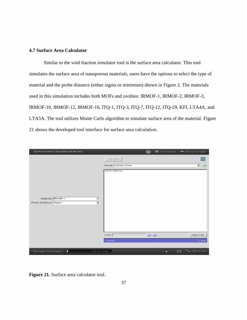
4.7 Surface Area Calculator

Similar to the void fraction simulator tool is the surface area calculator. This tool

simulates the surface area of nanoporous materials, users have the options to select the type of

material and the probe distance (either sigma or minimum) shown in Figure 2. The materials

used in this simulation includes both MOFs and zeolites: IRMOF-1, IRMOF-2, IRMOF-3,

IRMOF-10, IRMOF-12, IRMOF-16, ITQ-1, ITQ-3, ITQ-7, ITQ-12, ITQ-29, KFI, LTA4A, and

LTA5A. The tool utilizes Monte Carlo algorithm to simulate surface area of the material. Figure

21 shows the developed tool interface for surface area calculation.

Figure 21. Surface area calculator tool.

38

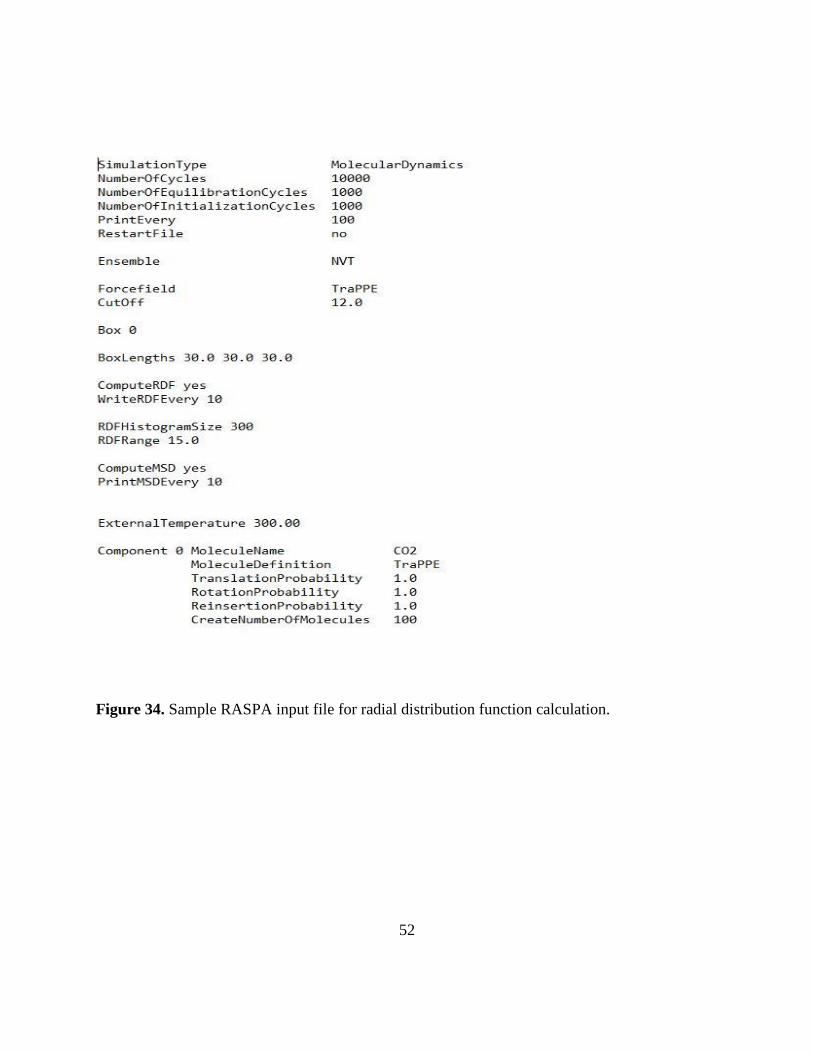
4.8 Radial Distribution Function Calculator

This tool simulates the radial distribution function of gases. The gases used for the

simulation include: methane, ethane, propane, butane, nitrogen, and carbon dioxide. The tool

allows the user to select (from a drop list) the type of gas to be used for the simulation. It also

allows the user to enter the simulation temperature. Using molecular dynamics with the NVT

ensemble, the tool performs the simulation and outputs a graph of the radial distribution function

versus distance in Angstroms. It also outputs density, self-diffusion graph and the self-diffusion

constant of the gas molecule. Figure 22 shows the developed tool interface for radial distribution

function calculation.

Figure 22. Radial distribution function calculator tool.

39

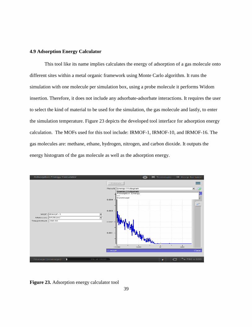
4.9 Adsorption Energy Calculator

This tool like its name implies calculates the energy of adsorption of a gas molecule onto

different sites within a metal organic framework using Monte Carlo algorithm. It runs the

simulation with one molecule per simulation box, using a probe molecule it performs Widom

insertion. Therefore, it does not include any adsorbate-adsorbate interactions. It requires the user

to select the kind of material to be used for the simulation, the gas molecule and lastly, to enter

the simulation temperature. Figure 23 depicts the developed tool interface for adsorption energy

calculation. The MOFs used for this tool include: IRMOF-1, IRMOF-10, and IRMOF-16. The

gas molecules are: methane, ethane, hydrogen, nitrogen, and carbon dioxide. It outputs the

energy histogram of the gas molecule as well as the adsorption energy.

Figure 23. Adsorption energy calculator tool

40

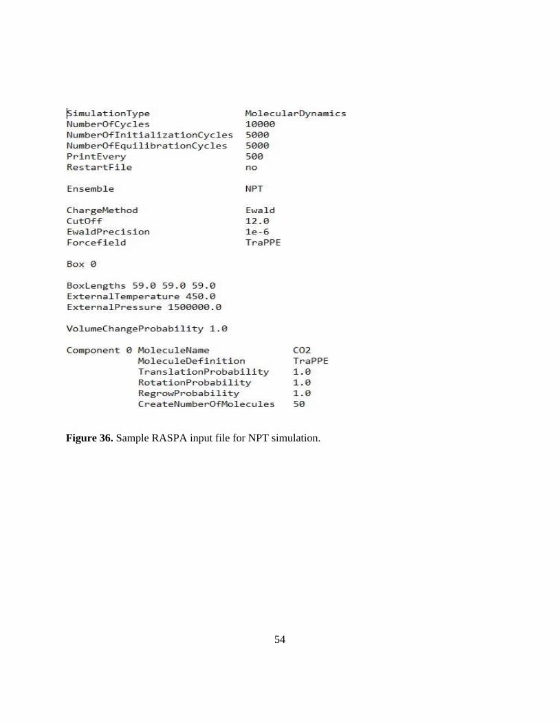
4.10 NPT Simulator

This tool utilizes molecular dynamic algorithm with the isobaric-isothermal ensemble

(NPT) to simulate the properties of gas molecules. To run a simulation, users are required to

select the molecule from a drop list, and enter the simulation temperature and pressure. The

molecules used in the tool include: methane, ethane, propane, and carbon dioxide. Figure 24

shows the developed tool interface for NPT simulation tool. The tool outputs the density and

total energy of the gas at the given conditions.

Figure 24. NPT simulator tool.

41

4.11 Gibbs Adsorption Simulator

This tool just like the previous adsorption tool simulates the adsorption of gas molecules

onto a metal organic framework. The difference between Gibbs ensemble adsorption simulation

and the adsorption simulation using grand canonical ensemble (μVT) is that Gibbs ensemble

adsorption uses two boxes for the simulation. The framework is contained in one box and a gas

phase in the other box. The simulation computes the adsorption using the forcefield without

requiring a fugacity coefficient or an equation of state. (Adsorption calculations using the grand

canonical ensemble require a fugacity coefficient that is not computed self-consistently from the

force field.) The MOFs used for this tool include: IRMOF-1, IRMOF-10, and IRMOF-16. The

gas molecules include: methane, helium, hydrogen, nitrogen, and carbon dioxide. This tool is

similar to the grand canonical adsorption tool in terms of input parameters. The tool outputs the

average absolute adsorption of the gas molecule as is shown in Figure 25.

Figure 25. Gibbs adsorption tool.

42

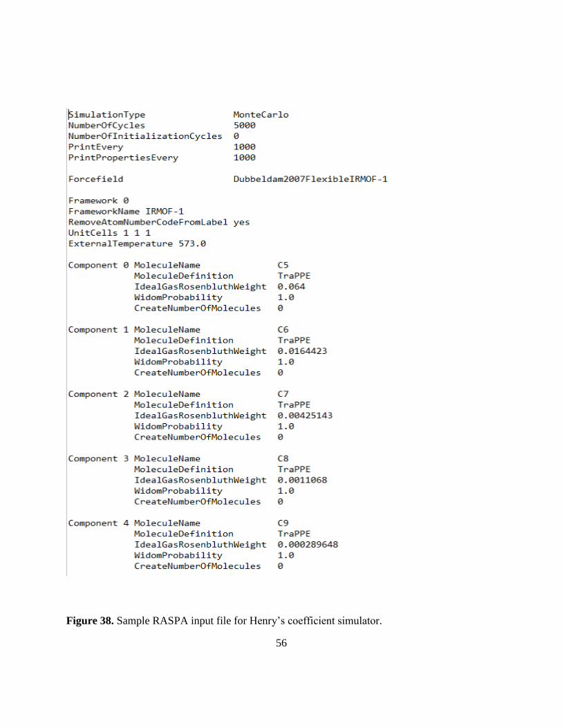
4.12 Henry’s Coefficients Simulator

This tool utilizes Monte Carlo algorithm with the Widom insertion to simulate henry

coefficients of n-alkane (n-pentane to n-nonane) for several nano porous materials. To run a

simulation, users are required to select the nanoporous material from a drop list. The nanoporous

material used in the tool include the metal organic frameworks IRMOF-1, IRMOF-10, IRMOF-

16, and the zeolite MFI_SI. Using a pre-calculated ideal gas Rosenbluth weight and temperature,

the tool outputs the Henry’s coefficients for the above mentioned normal alkanes as is depicted

in Figure 26.

Figure 26. Henry’s coefficient simulator tool.

43

CHAPTER 5. SUMMARY AND OUTLOOK

5.1 Summary

An approach to develop simulation tools on nanoHUB was presented here to show the

step-by-step method of tool development. The tools were developed in order to educate users on

how to successfully run molecular simulations most especially for diffusion and adsorption

calculations using RASPA. At the end of this project, twelve tools were successfully developed

and published alongside their pdf PowerPoint and description page explaining the highlights and

important concepts in the tool and the simulation in general. The tools developed include:

1. Gas Diffusion Coefficient in Metal Organic Frameworks

2. Gas Adsorption Calculator

3. VLE Simulator

4. Mixed Gas Adsorption Calculator

5. Mixed Gas Diffusion Calculator

6. Void Fraction Calculator

7. Surface Area Calculator

8. Radial Distribution Function Calculator

9. Adsorption Energy Calculator

10. NPT Simulator

11. Gibbs Adsorption Simulator

12. Henry’s Coefficients simulator

44

It is pertinent to state that the tools developed for this project are only to be used for

learning purposes. They are not to be used for research as the tools are setup to run and produce

results in a short timeframe thus making the simulations less rigorous. Each tool developed on

this project has no more than 5000 initialization cycles and 10000 production cycles. Increasing

the running cycles of the tool increases its accuracy but also increases the computational cost

(time). An increase in computational time is undesirable, because users would be less inclined to

run a simulation for more than a couple of minutes.

45

5.2 Outlook

The project documented in this thesis has shown how to develop tools on nanoHUB using

Python; for any tool that might be developed in the future, Jupyter notebook would be considered

as the tool development platform as this has advantages over the traditional Python developed

nanoHUB tools. Jupyter notebook has more functionality than and also serves as an integrated

development environment (IDE) which makes code writing and editing easier than writing on a

notepad.

Additionally, other tools that could be explored in the future include adsorption and

diffusion calculations using flexible metal organic frameworks. RASPA currently has the ability

to run simulations using flexible frameworks,18 but this was not treated here because RASPA

program is not parallelized and as such treating framework flexibility would be computationally

expensive. Similarly, none of the simulations here included the use of polarizable forcefields.

This is due to the fact that polarizability is not handled very well by the current RASPA code,

and is also computationally expensive. This could be included in future tools if the RASPA

software developers come up with an updated parallelized version of the software.

Finally, developing future tools with the ability to integrate visual aids such as iRASPA

which is a visualization package with editing capabilities54 would help users understand the

simulation tool and the different concepts the developer is trying to teach.

46

APPENDIX A

SCREENSHOT OF SAMPLE RASPA INPUT FILE FOR ALL TOOLS

This section contains sample RASPA input files for all tools developed. This is aimed at

showing users how to set up the calculations in RASPA.

Figure 27. Sample RASPA input file for adsorption isotherm calculation.

47

Figure 28. Sample RASPA input file for diffusion constant calculation.

48

Figure 29. Sample RASPA input file for VLE calculation.

49

Figure 30. Sample RASPA input file for mixed gas adsorption calculation.

50

Figure 31. Sample RASPA input file for mixed gas diffusion calculation.

51

Figure 32. Sample RASPA input file for void fraction calculation.

Figure 33. Sample RASPA input file for surface area calculation for MOF.

52

Figure 34. Sample RASPA input file for radial distribution function calculation.

53

Figure 35. Sample RASPA input file for adsorption energy calculation.

54

Figure 36. Sample RASPA input file for NPT simulation.

55

Figure 37. Sample RASPA input file for Gibbs adsorption calculation.

56

Figure 38. Sample RASPA input file for Henry’s coefficient simulator.

57

APPENDIX B

SAMPLE MAIN.PY FILES FROM WORKSPACE AND FROM REPOSITORY

This section compares the main.py file for the same tool (void fraction calculation) from

when the tool is developed on workspace using Rappture toolkit to when it is uploaded and

published on nanoHUB.

Figure 39. Sample skeleton file (main.py) generated by Rappture toolkit.

58

Figure 40. Sample main.py file for void fraction calculator tool for workspace.

59

Figure 40 continued.

60

Figure 41. Sample main.py file for void fraction calculator tool for nanoHUB repository.

61

Figure 41 continued.

62

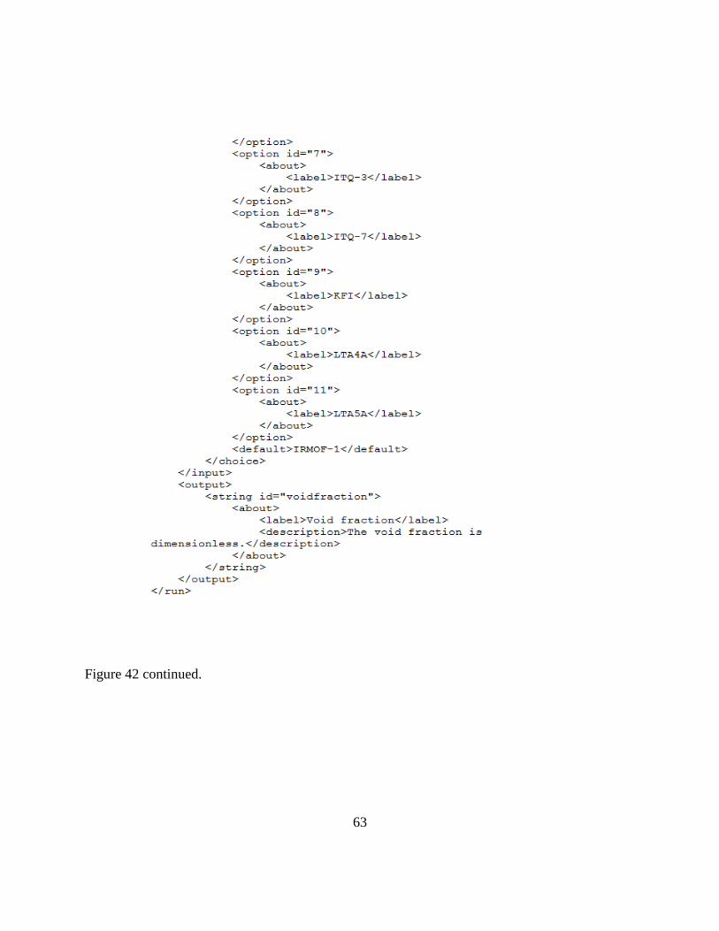
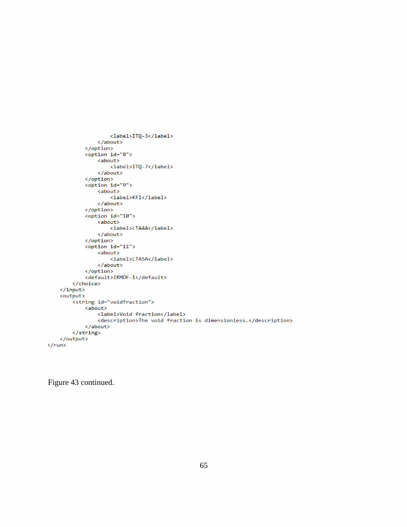
APPENDIX C

SAMPLE TOOL.XML FILES FROM WORKSPACE AND FROM REPOSITORY

Similar to the previous section, this section compares the tool.xml file for the same tool

(void fraction calculation) from when the tool is developed on workspace using Rappture toolkit

to when it is uploaded and published on nanoHUB.

Figure 42. Sample tool.xml file for void fraction calculator tool for workspace.

63

Figure 42 continued.

64

Figure 43. Sample tool.xml file for void fraction calculator tool for nanoHUB repository.

65

Figure 43 continued.

66

REFERENCES

1. Klimeck, G.; McLennan, M.; Brophy, S. P.; Adams III, G. B.; Lundstrom, M. S.,

nanoHUB.org: Advancing education and research in nanotechnology. Comput. Sci. Eng. 2008,

10, 17 - 23.

2. Kadioglu, O.; Keskin, S., Efficient separation of helium from methane using MOF

membranes. Sep. Purif. Technol. 2018, 191, 192 - 199.

3. Faltens, T. A.; Bermel, P.; Buckles, A.; Douglas, K. A.; Strachan, A.; Zentner, L. K.;

Klimeck, G., nanoHUB.org: A gateway to undergraduate simulation-based research in materials

science and related fields. Mater. Res. Soc Symp Proc. 2015, 1762.

4. Dubbeldam, D.; Calero, S.; Ellis, D. E.; Snurr, R. Q., RASPA: molecular simulation

software for adsorption and diffusion in flexible nanoporous materials. Mol. Simulat. 2016, 42,

81-101.

5. Zhang, J.; Clennell, M.; Dewhurst, D.; Liu, K., Combined Monte Carlo and molecular

dynamics simulation of methane adsorption on dry and moist coal. Fuel. 2014, 122, 186-197.

6. Bürgi, R.; Kollman, P. A.; van Gunsteren, W. F., Simulating proteins at constant pH: An

approach combining molecular dynamics and Monte Carlo simulation. Proteins. 2002, 47, 469-

480.

7. Chiu, S. W.; Jakobsson, E.; Scott, H. L., Combined Monte Carlo and molecular

dynamics simulation of hydrated lipid-cholesterol lipid bilayers at low cholesterol concentration.

Biophys. J. 2001, 80, 1104-14.

8. Hirotani, A.; Mizukami, K.; Miura, R.; Takaba, H.; Miya, T.; Fahmi, A.; Stirling, A.;

Kubo, M.; Miyamoto, A., Grand canonical Monte Carlo simulation of the adsorption of CO2 on

silicalite and NaZSM-5. Appl. Surf. Sci. 1997, 120, 81-84.

9. Gao, G.; Wang, W., Gibbs Ensemble Monte Carlo simulation of binary vapor-liquid

equilibria for CFC alternatives. Fluid Ph. Equilibria 1997, 130, 157-166.

10. Slepoy, A.; Thompson, A. P.; Plimpton, S. J., A constant-time kinetic Monte Carlo

algorithm for simulation of large biochemical reaction networks. J. of Chem. Phys. 2008, 128,

205101.

11. Dubbeldam, D.; Calero, S.; Vlugt, T. J. H.; Ellis, D. E.; Snurr, R. Q. RASPA: molecular

software package for adsorption and diffusion in (flexible) nanoporous materials.

https://github.com/numat/RASPA2 (accessed October 2019).

67

12. Dubbeldam, D.; Torres-Knoop, A.; Walton, K. S., On the inner workings of Monte Carlo

codes. Mol. Simul. 2013, 39, 1253-1292.

13. Dove, M. T., An introduction to atomistic simulation methods. Seminarios de la SEM

2008, 4, 7-37.

14. Abouelnasr, M. K. F.; Smit, B., Diffusion in confinement: kinetic simulations of self- and

collective diffusion behavior of adsorbed gases. Phys.Chem. Chem.Phys. 2012, 14, 11600-11609.

15. Werder, T.; Walther, J. H.; Jaffe, R. L.; Halicioglu, T.; Koumoutsakos, P., On the

water−carbon interaction for use in molecular dynamics simulations of graphite and carbon

nanotubes. J. Phys.Chem. B. 2003, 107, 1345-1352.

16. Henry, A. S.; Chen, G., Spectral phonon transport properties of silicon based on

molecular dynamics simulations and lattice dynamics. J. Comput. Theor. Nanos. 2008, 5, 141-

152.

17. Karplus, M.; McCammon, J. A., Molecular dynamics simulations of biomolecules. Nat.

Struct. Biol. 2002, 9, 646-652.

18. Dubbeldam, D.; Calero, S.; Ellis, D. E.; Snurr, R. Q., RASPA: molecular simulation

software for adsorption and diffusion in flexible nanoporous materials. Mol. Simul. 2016, 42, 81-

101.

19. Skoulidas, A. I.; Sholl, D. S., Self-diffusion and transport diffusion of light gases in

metal-organic framework materials assessed using molecular dynamics simulations. J. Phys.

Chem. B. 2005, 109, 15760-15768.

20. Greathouse, J. A.; Allendorf, M. D., Force field validation for molecular dynamics

simulations of IRMOF-1 and other isoreticular zinc carboxylate coordination polymers. J. Phys.

Chem. C. 2008, 112 , 5795-5802.

21. Bristow, J. K.; Tiana, D.; Walsh, A., Transferable force field for metal-organic

frameworks from first-principles: BTW-FF. J. Chem. Theory Comput. 2014, 10, 4644-4652.

22. Lin, L. C.; Lee, K.; Gagliardi, L.; Neaton, J. B.; Smit, B., Force-field development from

electronic structure calculations with periodic boundary conditions: applications to gaseous

adsorption and transport in metal-organic frameworks. J. Chem. Theory Comput. 2014, 10, 1477-

1488.

23. Rappe, A. K.; Casewit, C. J.; Colwell, K. S.; Goddard, W. A.; Skiff, W. M., UFF, a full

periodic-table force-field for molecular mechanics and molecular-dynamics simulations. J. Am.

Chem. Soc. 1992, 114, 10024-10035.

68

24. Vanommeslaeghe, K.; Raman, E. P.; MacKerell, A. D., Automation of the CHARMM

General Force Field (CGenFF) II: assignment of bonded parameters and partial atomic charges.

J. Chem. Inf Model. 2012, 52, 3155-3168.

25. Jorgensen, W. L.; McDonald, N. A., Development of an all-atom force field for

heterocycles. Properties of liquid pyridine and diazenes. J. Mol. Struc-Theochem. 1998, 424,

145-155.

26. Brdarski, S.; Karlström, G., Modeling of the Exchange Repulsion Energy. J. Phys. Chem.

A. 1998, 102, 8182-8192.

27. Halgren, T. A.; Damm, W., Polarizable force fields. Curr. Opin. Struct. Biol. 2001, 11,

236-242.

28. Shi, Y.; Xia, Z.; Zhang, J. J.; Best, R.; Wu, C. J.; Ponder, J. W.; Ren, P. Y.,

Polarizable atomic multipole-based AMOEBA force field for proteins. J. Chem. Theory Comput.

2013, 9, 4046-4063.

29. Wang, L. P.; Chen, J. H.; Van Voorhis, T., systematic parametrization of polarizable

force fields from quantum chemistry data. J. Chem. Theory Comput. 2013, 9, 452-460.

30. Borodin, O., Polarizable force field development and molecular dynamics simulations of

ionic liquids. J. Phys. Chem. B. 2009, 113, 11463-11478.

31. Cieplak, P.; Dupradeau, F. Y.; Duan, Y.; Wang, J. M., Polarization effects in molecular

mechanical force fields. J. Phys. Condens. Matter. 2009, 21, 1-21.

32. Warshel, A.; Kato, M.; Pisliakov, A. V., Polarizable force fields: history, test cases, and

prospects. J. Chem. Theory Comput. 2007, 3, 2034-2045.

33. Marques, M. A. L.; Castro, A.; Malloci, G.; Mulas, G.; Botti, S., Efficient calculation of

van der Waals dispersion coefficients with time-dependent density functional theory in real time:

Application to polycyclic aromatic hydrocarbons. J. Chem. Phys. 2007, 127, 014107.

34. Manz, T. A.; Chen, T.; Cole, D. J.; Gabaldon Limas, N.; Fiszbein, B., New scaling

relations to compute atom-in-material polarizabilities and dispersion coefficients : part 1. Theory

and accuracy. submitted to RSC Advances 2019.

35. Grimme, S.; Hansen, A.; Brandenburg, J. G.; Bannwarth, C., Dispersion-corrected

mean-field electronic structure methods. Chem. Rev. 2016, 116, 5105-5154.

36. Ambrosetti, A.; Ferri, N.; DiStasio, R. A.; Tkatchenko, A., Wavelike charge density

fluctuations and van der Waals interactions at the nanoscale. Science. 2016, 351, 1171-1176.

69

37. Hermann, J.; DiStasio, R.; Tkatchenko, A., First-Principles models for van der waals

interactions in molecules and materials: concepts, theory, and applications. Chem. Rev. 2017,

117 (6), 4714-4758.

38. Misquitta, A. J.; Stone, A. J., ISA-Pol: distributed polarizabilities and dispersion models

from a basis-space implementation of the iterated stockholder atoms procedure. Theor. Chem.

Acc. 2018, 137, 153.

39. Kaplan, I. G., Intertermolecular Interactions: Physical Picture, Computational Methods

and Model Potentials. John Wiley & Sons, Ltd: 2006; p 380.

40. Boda, D.; Henderson, D., The effects of deviations from Lorentz–Berthelot rules on the

properties of a simple mixture. Mol. Phys. 2008, 106, 2367-2370.

41. Garcia-Perez, E.; Serra-Crespo, P.; Hamad, S.; Kapteijn, F.; Gascon, J., Molecular

simulation of gas adsorption and diffusion in a breathing MOF using a rigid force field. Phys.

Chem. Chem. Phys. 2014, 16, 16060-6.

42. Ford, D. C.; Dubbeldam, D.; Snurr, R. Q.; Künzel, V.; Wehring, M.; Stallmach, F.;

Kärger, J.; Müller, U., Self-diffusion of chain molecules in the metal–organic framework

IRMOF-1: Simulation and experiment. J. Phys. Chem. Lett. 2012, 3, 930-933.

43. Eggimann, B. L.; Sunnarborg, A. J.; Stern, H. D.; Bliss, A. P.; Siepmann, J. I., An

online parameter and property database for the TraPPE force field. Mol. Simulat. 2014, 40 (1-3),

101-105.

44. Martin, M. G.; Siepmann, I. J., Transferable potentials for phase equilibria. 1. United-

atom description of n-Alkanes. Phys. Chem. 1998, 102, 2569-2577.

45. Chen, B.; Siepmann, I. J., Transferable potentials for phase equilibria. 3. Explicit-

hydrogen description of normal alkanes. J. Phys. Chem. 1999, 103, 5370-5379.

46. (2013)"Workspace,"https://nanohub.org/resources/workspace. (DOI:

10.4231/D3C24QN4W).

47. McLennan, M. "The Rappture Toolkit," http://rappture.org.

48. (2019) "Apache Subversion", https://subversion.apache.org.

49. (2019) "Tortoise SVN", https://tortoisesvn.net.

70

50. Dubbeldam, D.; Walton, K. S.; Ellis, D. E.; Snurr, R. Q., Exceptional negative thermal

expansion in isoreticular metal-organic frameworks. Angew. Chem.-Int. Ed. 2007, 46, 4496-

4499.

51. Keskin, S.; Sholl, D. S., Assessment of a metal-organic framework membrane for gas

separations using atomically detailed calculations: CO2, CH4, N2, H2 mixtures in MOF-5. Ind.

Eng. Chem. Res. 2009, 48, 914-922.

52. Liu, D. H.; Zheng, C. C.; Yang, Q. Y.; Zhong, C. L., Understanding the adsorption and

diffusion of carbon dioxide in zeolitic imidazolate frameworks: A molecular simulation study. J.

Phys. Chem. C 2009, 113, 5004-5009.

53. Potoff, J. J.; Siepmann, J. I., Vapor–liquid equilibria of mixtures containing alkanes,

carbon dioxide, and nitrogen. AIChE J. 2001, 47, 1676-1682.

54. Dubbeldam, D.; Calero, S.; Vlugt, T. J. H., iRASPA: GPU-accelerated visualization

software for materials scientists. Mol. Simulat. 2018, 44, 653-676.