1

Determinants of Food Security in Southern Ethiopia

By Shiferaw Feleke, Richard L. Kilmer and Christy Gladwin PO Box 110240

Food and Resource Economics Department Institute of Food and Agricultural Sciences

University of Florida Gainesville, Florida 32611-0240

Kilmer@UFL.EDU

May 12, 2003

A selected Paper Presented at the 2003 American Agricultural Economics Association Meetings in Montreal, Canada

Abstract: The study investigates the relative importance of supply-side and demand-side factors of household food security through a logistic regression analysis applied to data collected from 247 sample households in Southern Ethiopia. Among the nine factors included in the model, seven were identified as statistically significant determinants of household food security: technological adoption, farming system, farm size, land quality, household size, per capita aggregate production and access to market. Among these, technological adoption, farming system, farm size, and land quality are supply-side factors. Household size, per capita aggregate production, and access to market are demand-side factors. Based on the magnitude of their partial effects on the probability of food security, supply-side factors are more powerful than the demand-side factors in determining household food security, implying that interventions focused on these factors need to get priority attention by policy, research and extension.

Keywords: Development, Ethiopia, household, food security

Copyright 2003 by Shiferaw Feleke, Richard L. Kilmer and Christy Gladwin. All rights reserved. Readers may make verbatim copies of this document for non-commercial purposes by

any means, provided that this copyright notice appears on all such copies.

2

Determinants of Food Security in Southern Ethiopia

Introduction

In the early 1980s, a paradigm shift occurred in the field of food security, following

Amartya Sen (1981)’s claims that food security is more of a demand concern, affecting the poor’s

access to food, than a supply concern, affecting availability of food at the national level. Since

then, accepted wisdom has defined food security as being primarily a problem of access to food.

Farmers’ own production became viewed as a route to entitlement, either directly via their own

supplies of food, or indirectly via lower market prices for consumers (Maxwell S., 1996). At the

same time, the unit of analysis shifted from the global and national level to the household and

individual level. In 1986, the World Bank (1986:1) defined food security as “access by all people

at all times to enough food for an active and healthy life.”

Despite the wide acceptance of Sen’s thinking, early concerns about adequate supplies of

food and national food self-sufficiency live on today in the preoccupation of many governments, in

Africa in particular, with national food self-sufficiency (Harsch, 1992). Yet, food self-sufficiency

is neither a necessary nor a sufficient condition for food security (Cleaver, 1993). It is not a

necessary condition because food imports can be used to fill the gap between domestic production

and consumption. It is not a sufficient condition because even when a country is sufficient, there

may still be significant number of people facing food insecurity.

Recently, however, the entitlement approach has evoked many criticisms in academic

circles (Sijm, 1997). The most important criticism is that it underestimates the importance of

supply-side factors. Consequently, by focusing attention only on improving the distribution of

food via inappropriate institutional changes or depressed consumer prices, policy makers might

3

neglect to make necessary improvements in the food supply that would eventually drive prices of

food down for the poor and make food more affordable (Sijm, 1997).

This study attempts to investigate the relative importance of supply-side versus demand-

side factors in influencing food security in southern Ethiopia at the household level. Objectives

are to (1) identify the determinants of food security in southern Ethiopia at the household level, (2)

assess the relative importance of the determinants of food security, and (3) suggest entry points for

research, extension and policy interventions.

Food Insecurity in Ethiopia

Over the past three decades, Ethiopia has been challenged by lack of food security. In

Ethiopia, the trend in growth of domestic food production matched population growth only in the

1960s (Markos, 1997). The per capita domestic food production has steadily declined over the

last three decades. Between 1971 and 2000, a simple average of year-to-year growth of per

capita production was –1.15 percent with average growth rates during the 1970s, 1980s and

1990s estimated at -0.84, -1.98 and -0.64 percent, respectively (FAO, 2001).

Ethiopia is among the poorest and most food insecure countries of the world. On the

Human Development Index (HDI) of the United Nations Development Program (UNDP), it

ranks 171st out of 174 countries in the world, and about 60 percent of its population live below

the poverty line (FAO, 2001). In terms of food security, it is one of the seven African countries

that constitute half of the food insecure population in Sub-Saharan Africa (Sisay, 1995). Average

caloric intake in rural areas is 1,750 calories/person/day (FAO, 1998), which is far below the

medically recommended minimum daily intake of 2100 calories/person/day. As a result, about

51 percent of the population are undernourished (FAO, 2001). In 1994, infant and child

4

mortality rates were 118 and 173 per 1000, respectively; maternal mortality rate was 700 per

10,000; and life expectancy at birth during the same year was 50 years (MEDAC, 2000).

The mainstay of the Ethiopian economy is agriculture that generates 50 percent of the

GDP, 90 percent of the foreign exchange earnings, and provides 80 percent of employment.

Ethiopia is the second most populous nation in Sub-Saharan Africa with a population of about 67

million of which 85 percent are rural (FAO, 2002). By the definition of Tomich et al. (1995),

Ethiopia is a CARL (a country of abundant rural labor force), and at an early stage of structural

transformation.

Food insecurity and poverty in Ethiopia are attributed to the poor performance of the

agricultural sector, which in turn is attributed to both policy and non-policy factors (Wolday,

1995). Among the non-policy factors, recurrent drought is mentioned as the number one cause of

food shortage in Ethiopia. Among the non-policy factors are some ill-conceived development

policies that were implemented by past regimes in the years before 1991.

Theoretical Model

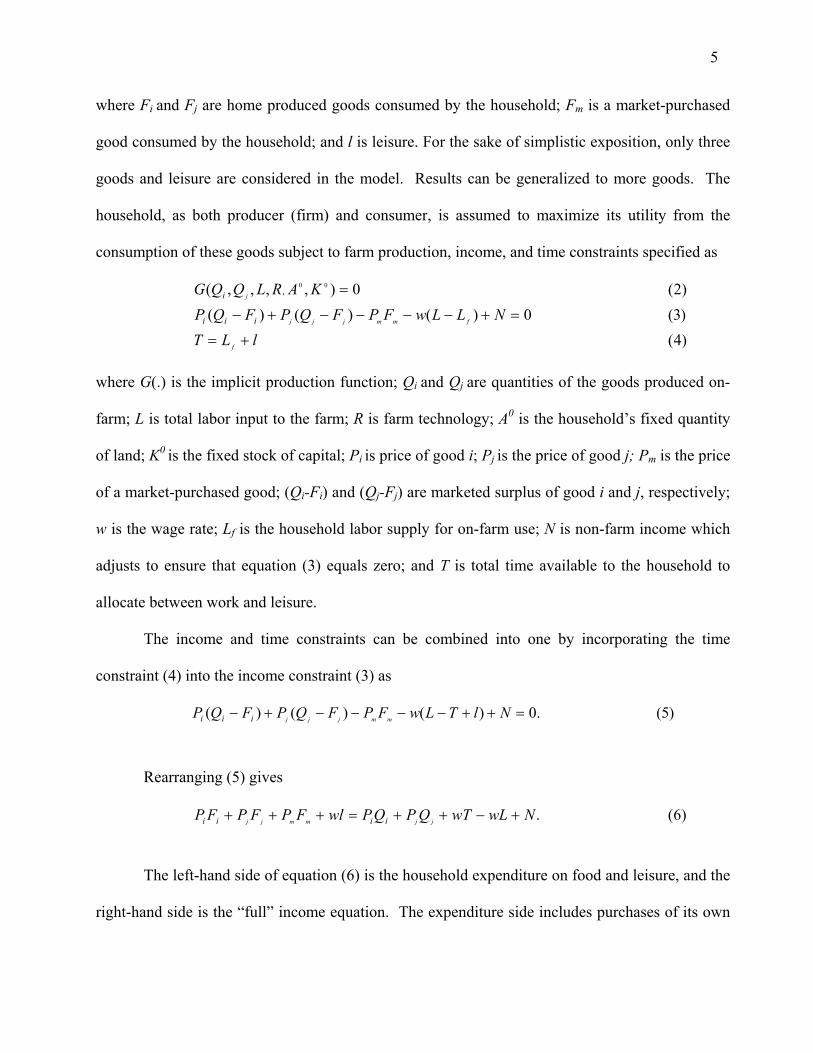
Following the modeling of production and consumption behaviors of a rural household by

Straus (1983), Barnum and Squire (1979), and Yotopoulos (1983), the extent of household food

security in this study is modeled within the framework of consumer demand and production

theories. Households derive utility from the consumption of foods through the satisfaction found

in a set of taste characteristics as well as the health effects of the nutrients consumed. Among the

various nutrients derived from the consumption of foods, only calories are considered in this study.

Following Strauss (1983), the household utility function in this study is specified as

)1(),,,( lFFFUU mji=

5

where Fi and Fj are home produced goods consumed by the household; Fm is a market-purchased

good consumed by the household; and l is leisure. For the sake of simplistic exposition, only three

goods and leisure are considered in the model. Results can be generalized to more goods. The

household, as both producer (firm) and consumer, is assumed to maximize its utility from the

consumption of these goods subject to farm production, income, and time constraints specified as

)4( )3(0)()()()2(0),,,,( 00

,

lLTNLLwFPFQPFQP

KARLQQG

f

fmmjjj

j

iii

i

+=

=+−−−−+−

=

where G(.) is the implicit production function; Qi and Qj are quantities of the goods produced on-

farm; L is total labor input to the farm; R is farm technology; A0 is the household’s fixed quantity

of land; K0 is the fixed stock of capital; Pi is price of good i; Pj is the price of good j; Pm is the price

of a market-purchased good; (Qi-Fi) and (Qj-Fj) are marketed surplus of good i and j, respectively;

w is the wage rate; Lf is the household labor supply for on-farm use; N is non-farm income which

adjusts to ensure that equation (3) equals zero; and T is total time available to the household to

allocate between work and leisure.

The income and time constraints can be combined into one by incorporating the time

constraint (4) into the income constraint (3) as

)5(.0)()()( =++−−−−+− NlTLwFPFQPFQP mmjjjiii

Rearranging (5) gives

)6(.NwLwTQPQPwlFPFPFP jjmmjj iiii +−++=+++

The left-hand side of equation (6) is the household expenditure on food and leisure, and the

right-hand side is the “full” income equation. The expenditure side includes purchases of its own

6

farm-produced good i (PiFi), the household’s purchase of its own farm-produced good j (PjFj), the

household’s purchase of the market good (PmFm), and the household purchase of its own leisure

time (wl). The full income side consists of the value of total agricultural production PiQi and PjQj,

the value of the household’s entitlement of time wT, the value of labor on the farm including hired

labor wL, and non-farm income N.

The lagrangian is

)7()].,,,,,([)]()[(),,,(

00 KARLQQGwlFPFPFPNwLwTQPQPlFFFUMax

jimmjjii

jjiimji

µλψ

++++

−+−+++=

Following Strauss (1983, p.4), from the first order conditions the relationship between

production and consumption can be established as

)9(

)8(

i

j

j

i

j

i

j

i

i

i

i

i

QQ

QG

QG

PP

FU

FU

LQ

QG

LG

Pw

FU

lU

∂

∂−=

∂∂

∂∂

==

∂∂

∂∂

∂∂

=

∂∂

∂∂−

==

∂∂

∂∂

An important property of this model is its recursiveness in the sense that production

decisions are made first and subsequently used in allocating the full income between consumption

of goods and leisure (Strauss, 1983). The decision on consumption of the bundle (Fi,Fj) is

influenced by the decision to produce the quantities (Qi, Qj ) (Figure 1). Also, this model assumes

that markets exist for both goods and inputs.

7

As a consumer, the household maximizes its utility by equating (equation (8)) the marginal

rate of substitution between leisure and consumption of good i to w/Pi (point Q’i in Figure 2) to the

marginal product of labor at L’ (Figure 2). The output in excess of point Q’i is sold (Qi-Q’i in

Figure 2). In the same figure, we see that the amount of labor the household supplies (L) falls

short of the quantity of labor demanded (L’) where the marginal product is equal to the ratio w/Pi

(point L’). Hence, it hires additional labor (L’-L) until the ratio w/Pi is equal to the marginal

product, which is at point QiL (Figure 2). The household’s supply of labor is determined by the

opportunity cost of taking leisure, which is expressed in terms of the marginal product forgone.

The higher the ratio w/Pi, the greater is the opportunity cost of taking leisure. The household

continues to supply labor until the marginal rate of substitution between leisure and the

consumption good i is equal to the relative market prices of the same (at point Qi’L in Figure 2).

In equation (9), the household maximizes its utility by equating the marginal rate of

substitution between the two goods (Fi and Fj) to the price ratio of the same (point (Fi, Fj ) in

Figure 1). At that point, it is efficient in consumption. However, given its production possibility

curve (PP’), this level of consumption is unattainable without trade. With the given production

possibility curve PP’, the household is efficient in terms of production at point QiQj where it

maximizes its profits by equating the marginal rate of transformation to the same price ratios

(Figure 1). In order to attain the level of consumption (Fi, Fj), it has to trade. Hence, it purchases

Fj-Qj of good j, and sells Qi-Fi of good i. Similarly, in equation (8), the household as a producer

equates the marginal product of labor to the ratio w/Pi (point L’ in Figure 2).

Following Strauss (1983), we can mathematically derive the production side and

consumption-side equations separately. Starting with the production side, the first order conditions

8

can be solved for the input demand (L*) and output supply (Q*) in terms of all prices, the wage

rate, technology, fixed land, and capital as

)10(),,,,,( 00** KARwPPLL ji=

and

)11(),,,,,( 00** KARwPPQQ ji=

These solutions involve the decision rules for the quantities of labor input used and output

produced (production-side). Once the optimum level of labor is chosen, the value of full income

when profits have been maximized can be obtained by substituting L* and Q* into the right hand

side of the income constraint (equation 6) as

)12(**** NwLwTQPQPY jjii +−++=

and )13(),,,,,( 00** NKARwPPwTY ji ++= π

where Y* is the “full” income under the assumption of maximized profit π*.

The first order conditions can be solved for consumption demand in terms of prices, the

wage rate, and income as

)14(),,,,( *YwPPPFF mjikk =

where k = i, j, m.

These solutions involve the decision for the quantities of goods and leisure consumed

(consumption demand-side). The three equations (equations 10, 11 and 14) give us a complete

picture of the economic behavior of the farm household. They are combined through the profit

effect. This occurs in semi-subsistence households as the study region where income is

determined by the households’ production activities, implying that changes in factors influencing

9

production also changes income, which in turn affects consumption behavior. Incorporating

demographic factors (D), the demand for food indicated in equation 14 can be rewritten as

)15(]),,,,,(,,,,[ 00* DNKARwYwPPPFF mjikk =

where k = i, j, m.

Empirical Model

Having determined the demand for both home-produced and market-purchased goods, we

can now calculate the amount of calories (Ci) available in the respective food items. Given that the

indicator of food security is defined by calorie availability (Ci) and consumption needs of calories

γ, household food security is determined by the difference between calorie availabilities and needs.

The calorie availability is calculated from equation (15) using calorie conversion factors. The

needs are computed based on the requirement of the family members depending on age, sex, etc.

Defining Ci* = Ci - γi, where Ci is the calorie availability determined from equation (15) and

γ is the consumption needs for the ith household, Ci*>0 corresponds to the consumption demand

exceeding the household calorie needs while Ci* <0 corresponds to the consumption demand

failing to meet the household calorie needs. Hence, assuming a linear function, we can write the

unobserved calorie availability/consumption demand as

)16(1

*iij

kn

jji XC εβ += ∑

=

=

where Xij are explanatory variables indicated in equation (15) and εi is the error term.

The observed variable is food security where Zi=1 when Ci*>0 and Zi=0 when Ci

*<0 for

the ith household. The household observed to be food secure (Zi=1) has a consumption demand or

calorie availability greater than or equal to its needs, and the household observed to be food

insecure (Zi=0) has a consumption demand /calorie availability less than its needs.

10

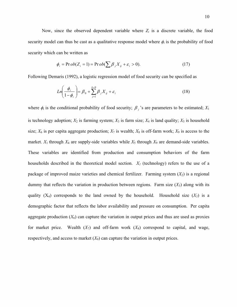
Now, since the observed dependent variable where Zi is a discrete variable, the food

security model can thus be cast as a qualitative response model where φi is the probability of food

security which can be written as

)17().0(Pr)1(Pr >+=== ∑ iijjii XobZob εβφ

Following Demaris (1992), a logistic regression model of food security can be specified as

)18(1

9

10 iij

k

jj

i

i XLn εββφ

φ++=

− ∑

=

=

where φi is the conditional probability of food security; jβ ’s are parameters to be estimated; X1

is technology adoption; X2 is farming system; X3 is farm size; X4 is land quality; X5 is household

size; X6 is per capita aggregate production; X7 is wealth; X8 is off-farm work; X9 is access to the

market. X1 through X4 are supply-side variables while X5 through X9 are demand-side variables.

These variables are identified from production and consumption behaviors of the farm

households described in the theoretical model section. X1 (technology) refers to the use of a

package of improved maize varieties and chemical fertilizer. Farming system (X2) is a regional

dummy that reflects the variation in production between regions. Farm size (X3) along with its

quality (X4) corresponds to the land owned by the household. Household size (X5) is a

demographic factor that reflects the labor availability and pressure on consumption. Per capita

aggregate production (X6) can capture the variation in output prices and thus are used as proxies

for market price. Wealth (X7) and off-farm work (X8) correspond to capital, and wage,

respectively, and access to market (X9) can capture the variation in output prices.

11

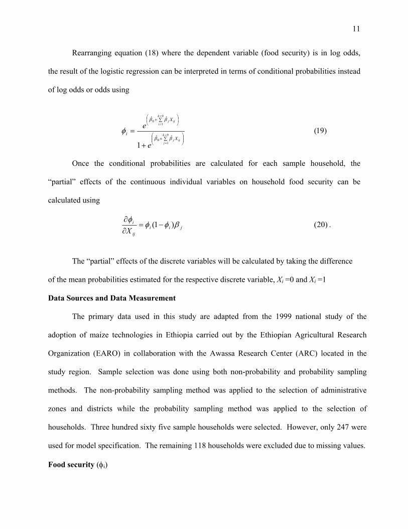
Rearranging equation (18) where the dependent variable (food security) is in log odds,

the result of the logistic regression can be interpreted in terms of conditional probabilities instead

of log odds or odds using

)19(

19

10

9

10

ˆˆ

ˆˆ

∑+

∑+

=

=

=

=

+

=k

jijj

k

iijj

X

X

i

e

eββ

ββ

φ

Once the conditional probabilities are calculated for each sample household, the

“partial” effects of the continuous individual variables on household food security can be

calculated using

)20()1( jiiij

i

Xβφφ

φ−=

∂∂

.

The “partial” effects of the discrete variables will be calculated by taking the difference

of the mean probabilities estimated for the respective discrete variable, Xi =0 and Xi =1

Data Sources and Data Measurement

The primary data used in this study are adapted from the 1999 national study of the

adoption of maize technologies in Ethiopia carried out by the Ethiopian Agricultural Research

Organization (EARO) in collaboration with the Awassa Research Center (ARC) located in the

study region. Sample selection was done using both non-probability and probability sampling

methods. The non-probability sampling method was applied to the selection of administrative

zones and districts while the probability sampling method was applied to the selection of

households. Three hundred sixty five sample households were selected. However, only 247 were

used for model specification. The remaining 118 households were excluded due to missing values.

Food security (φi)

12

Two objective methods of food security measurement have been widely used in most food

security studies. They are the consumption level of a given household during a given period and

the caloric content of a 24-hour diet recall. However, neither method provides a full assessment of

food security because they fail to take into account the vulnerability and sustainability elements of

food security and hence neither method has been accepted as a “gold standard” for an analysis of

household food security (See Maxwell D, 1996 for discussion of both methods).

The measurement of food security for this study is made in relation to the vulnerability

and unsustainability elements of food insecurity discussed in Maxwell D. (1996). The timing

and volume of maize harvest is chosen as an indicator, which can capture the vulnerability and

unsustainability elements food insecurity. Maize is chosen because it is the staple crop in both

cereal-based and cereal-enset-based systems of the study area. Normally, maize is harvested in

large quantities at maturity. However, because of the serious food shortage prior to the normal

harvesting season, the number of farmers harvesting maize in large quantities before maturity for

consumption or sale has been increasing and so are unsustainability and vulnerability to food

insecurity.

Based upon the timing and amount of maize harvested as a proxy to vulnerability and

unsustainablity in terms of food insecurity, households are classified into two groups. One group

consists of those households who harvest one-third to one-half or more of their maize before

maturity and another group consists of those households harvesting less than one-third of their

maize. The first group of households is most vulnerable and unsustainable and hence is

considered food insecure and the second is less vulnerable and capable of sustaining their

families form one season to the other and is considered as food secure. The variable is a

13

bivariate variable taking the value one when the household is food secure and zero when the

household is food insecure.

Technology adoption (X1)

Technology adoption refers to the use of high yielding varieties of maize along with

improved agronomic practices. Households who reported to have used this package of

technologies are considered as adopters (X1=1) and those who have never used this package of

technologies are considered as non-adopters (X1=0). Adoption is expected to increase food

security through its effect on raising food availability and income. The expected effect on food

security (φi) is positive.

Farming system (X2)

Farming system was determined based upon the location of the household in relation to

cereals-based versus cereal-enset-based sub-systems. Households residing in an area where

cereals are predominant belong to the cereals-based system. Households residing in an area

where both cereals and enset are grown with cereals as major and enset as secondary belong to

cereals-enset-based system. These two systems have their own distinctive production,

processing, storage, and marketing features, which have implications for household food

security. It is expected that households in cereals-enset-based systems are more likely to be food

secure than those in the cereal-based system because of the better productivity, longer storage

and flexible harvesting, drought tolerance and other desirable traits of the enset plant. Coding

the cereal-based system as zero (X2=0) and the cereal-enset-based system as one (X2=1), the

expected effect on food security (φi) is positive.

Farm size (X3)

14

Farm size is the total farmland owned by the household as measured in hectares. The

larger the farmland, the higher the production level. Hence, it is expected that households with

larger farmland are more likely to be food secure as opposed to those with small farmland. The

expected effect on food security (φi) is positive.

Land quality (X4)

Land quality is measured by the subjective judgment of the household about the fertility

of their land. The better the land quality the higher the production level. Households who

reported that their land requires chemical fertilizer take the value one (X4=0) and those who

reported that their land requires no chemical fertilizer to grow crops take the value zero (X4=1).

The expected effect on food security (φi) is positive.

Household size (X5)

Farm households in Ethiopia are small-scale semi-subsistence producers with limited

participation in the non-agricultural sector. Because resources are very limited, the increasing

family size may put much more pressure on consumption than it contributes to production. Food

requirements increase with the number of persons in a household. The expected sign is negative.

Per capita aggregate production (X6)

The per capita aggregate production consists of both crop and livestock production for

each study zone. It was computed by converting the outputs of the various crops and livestock

products into wheat equivalents. It is assumed that per capita aggregate production influences

household food security through the price effect. That is, an increase in per capita aggregate

production causes price to fall and hence those households whose income is dependent on food

crops face a fall in farm income. The higher the market supply, the lower the price, and hence

15

the higher the loss of producer revenue in the case of inelastic demand (Foster, 1992). Hence,

the expected effect on food security (φi) is negative.

Wealth (X7)

The wealth status of the household is measured by the number of livestock owned, since

livestock is the most important indicator of wealth in rural Ethiopia. A household’s level of farm

resources (e.g., livestock) can be expected to affect its ability to withstand abrupt changes in

production, prices, income, or unforeseen events that create the need for additional expenditures.

Particularly in Ethiopia where the incidence of crop failure frequently occurs due to rainfall

shortage, the level of one’s resources is very important to combat those incidences. The

expected effect on food security (φi) is positive.

Off-farm work (X8)

Off-farm work was measured based on whether or not the household has an off-farm job.

A household with an off-farm job takes the value zero and the household with an off-farm job

takes the value one. The expected effect on food security (φi) is positive.

Physical access to market (X9)

Physical access to the market was measured by the amount of time required to get to the

nearest local market. The longer the time it takes to get to the market, the less frequently the

farmer visits the market and hence less likely to get market information. When there is lack of

adequate information about prices, the farmers may sell at times when prices are low and buy

when prices are high. The expected effect on food security (φi) is negative.

Results and Discussion

Descriptive results

16

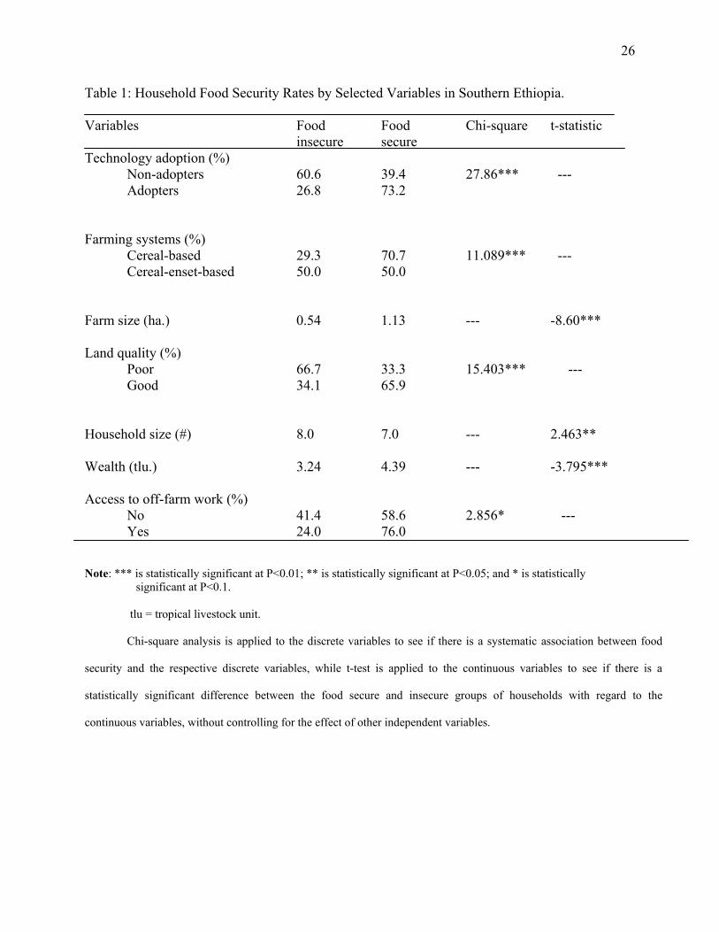
Household food security rates for selected household characteristics are presented in Table

1. The proportion of food secure households is higher among adopters (73 %) than among non-

adopters of improved seeds (39 %). The proportion of food secure households is higher in the

cereal-based system than in the cereal-enset-based farming system. The farm size of the food

secure households is significantly larger for the food secure than for the food insecure households

(p<0.01), implying that it matters in predicting who would be food secure. The average farm size

of food secure households is 1.13 ha while that of the food insecure households is only 0.54 ha. A

large difference is also observed in the proportion of food secure households with regard to land

quality. Food security rate is higher among households with good land quality.

Household size as measured by the number of persons in the household is higher for the

food insecure households as compared to that of the food secure households. On average, food

secure households have seven family members while food insecure households have eight family

members. The per capita food production of the food secure households is slightly higher than that

of the food insecure households. The overall average per capita aggregate production in the region

is 161 kilograms. Wealth as proxied by the livestock size is significantly larger for the food secure

than for the food insecure households (P<0.01), implying that it matters in predicting who would

be food secure. The average livestock size of food secure households is about four while that of

the food insecure households is three tropical livestock units. Physical access to the market as

proxied by the time spent to get to the nearest market center is also found to have an important

relationship with household food security. The longer the time it takes the household to get to the

nearest market the higher the food insecurity.

Model Characteristics

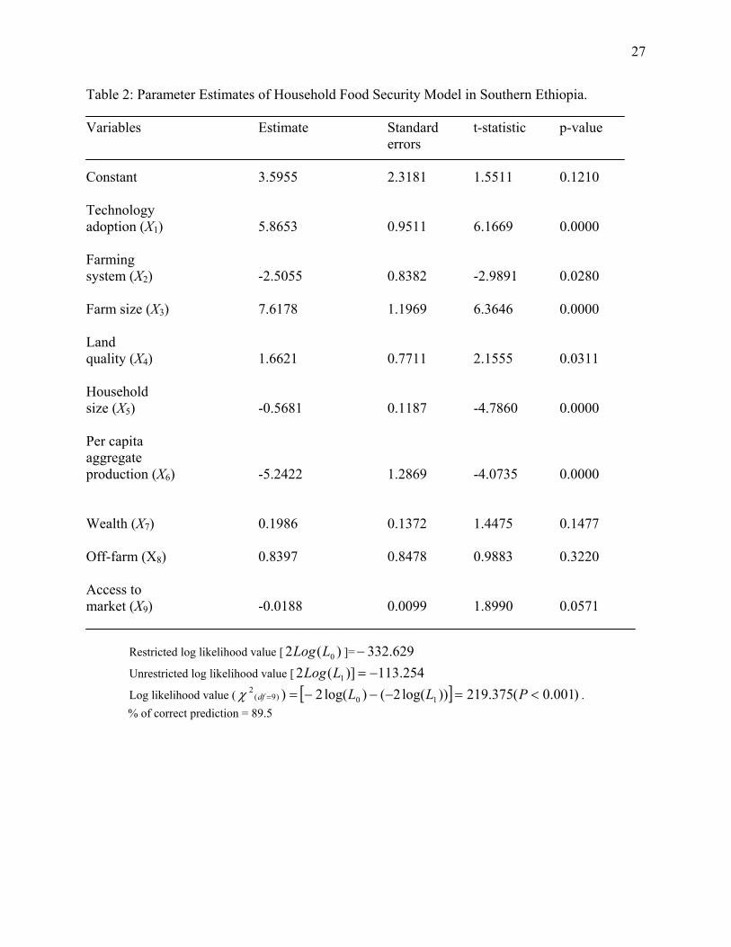
17

The likelihood ratio chi-square statistic is used to test the dependence of food security on

the selected variables in the model. Under the null hypothesis (H0) where we have only one

parameter, which is the intercept (β0), the value of the restricted log likelihood function is -332.629

while under the alternative hypothesis (H1) where we have all the parameters, the value of the

unrestricted log likelihood function is -113.254. The model chi-square statistic, which is the

difference of the values of the two log likelihood functions, is 219.375. It is highly significant

(P<0.001) with nine degrees of freedom, indicating that at least one of the parameters in the

equation is nonzero. Thus, the log odds of household food security is related to the independent

variables.

With regard to the predictive efficacy of the model, out of the 247 sample households

included in the model, 221 are correctly predicted or 89.5 percent prediction. Out of the 247

observed households in the sample, 148 are food secure (60%) of which 135 are correctly

predicted by the model, which is 91.2 percent prediction. Out of the 247 observed households, 99

are food insecure (40%) of which 86 are correctly predicted by the model, which is 86.9 percent

prediction. The chi-square showed a significant association between observed food

security/insecurity and model prediction of food security/insecurity (χ2=150.6; P<0.01).

Parameter Estimates of Determinants of Food Security

Among the nine factors considered in the model, seven were found to have a significant

impact in determining household food security (Table 2). These are technology adoption, farming

system, farm size, land quality, household size, per capita aggregate production, and access to

market. Among the significant factors, technology adoption, farming systems, farm size, and land

quality are supply-side determinants. Household size, per capita aggregate production, and market

access are demand-side determinants.

18

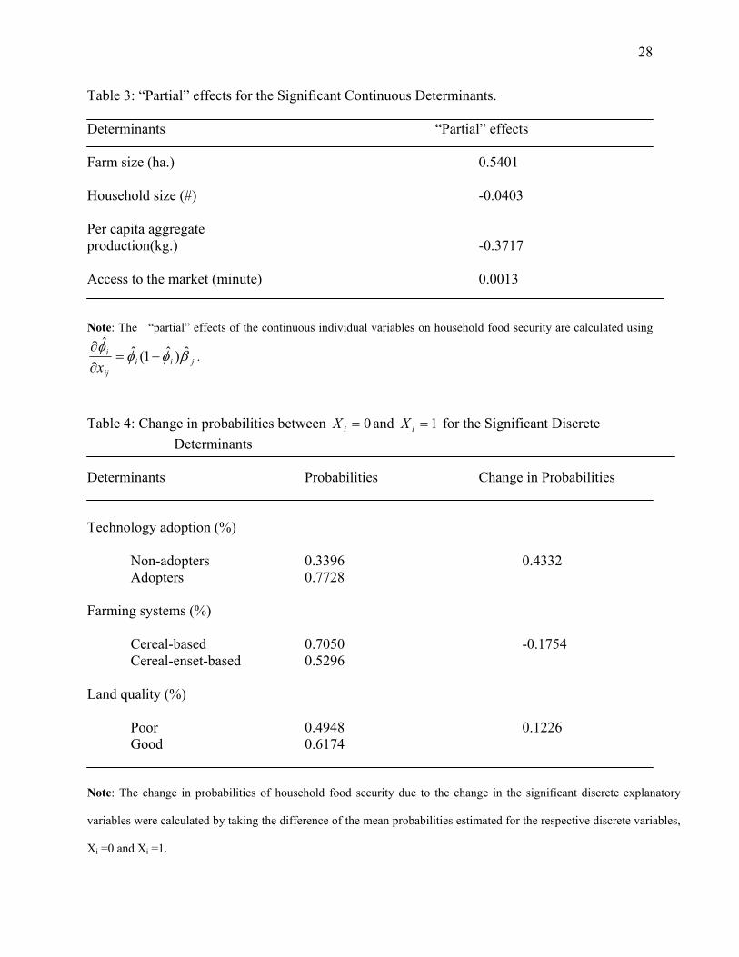
The magnitude of the effect of changes in statistically significant individual determinants

on household food security was assessed based upon the “partial” effects of the respective

variables on conditional probabilities (Table 3 & 4). The “partial” effects of the continuous

variables were calculated using equation (20) while those of the discrete variables were calculated

by taking the difference of the mean probabilities estimated for the respective discrete variable, Xi

=0 and Xi =1. The “partial” effects thus calculated from the logistic model show the effect of a

change in an individual variable on the probability of food security when all other exogenous

variables are held constant.

Supply-side Determinants

All the four supply-side factors included in the model (technology adoption, farming

system, farm size and land quality) were found to have a significant relationship with household

food security.

Technology adoption

Keeping the other variables in the model constant, technology adoption is positively and

significantly related to the probability of food security, implying that the likelihood of food

security increases with the farmers’ use of agricultural technologies. In other words, adopters of

improved seeds along with improved agronomic practices are more likely to be food secure than

non-adopters. A unit increase in adoption defined by the shift from non-adoption (X1=0) to

adoption (X1=1) increases the probability of food security from φ =0.3396 to φ =0.7728 (Table 4).

Such a significant effect of technology adoption on the probability of food security can be

explained in two ways. One is that the adoption of a package of high yielding varieties along with

improved agronomic practices directly increases food availability at the household level. The

19

second reason is related to the cash income effect. An adopter is better off than a non-adopter

because an adopter earns more income than a non-adopter because of the market surplus.

Farming system

A household in a cereal-based farming system is more likely to be food secure than that in

a cereal-enset based system. A unit change defined by the shift from a cereal-based system (X2=0)

to a cereal-enset based system (X2=1) decreases the probability of food security from φ =0.7050 to

φ =0.5296. In other words, households in the cereal-based farming system are more likely to be

food secure than those in the cereal-enset-based system.

Farm size

Another supply-side factor found to have a significant impact on household food security is

farm size. A positive and significant relationship is found between farm size and the probability of

food security, implying that the probability of food security increases with farm size. The “partial”

effect of a unit increase in farm size is 0.5401, indicating that the probability of food security

increases by 0.5401 for a one hectare increase in farm size (Table 3).

Land quality

Land quality is also another supply-side factor found to have a positive and significant

relationship with household food security. Households who have relatively fertile land are more

likely to be food secure than those with relatively less fertile land. A unit increase in land quality

defined by the shift in fertility from poor (X4=0) to good fertility condition (X4=1) increases the

probability of food security from φ =0.4948 to φ =0.6174.

Demand-side Determinants

20

Among the five demand-side factors included in the model, household size, market access,

and per capita aggregate production that is used as a proxy for prices were found to have a

significant relationship with household food security. Wealth and access to off-farm work were

not found to be statistically significant. However, their signs were as expected.

Household size

Household size has a negative and significant relationship with the probability of food

security, implying that the probability of food security decreases with family size. Each additional

increase in household size reduces the probability of food security by 0.04.

Per capita aggregate production

Per capita aggregate production is negatively and significantly related to the probability of

household food security. The “partial” effect of a unit increase in per capita aggregate production

on the conditional probability of food security is –0.3717. This means that each unit increase

(100kg) in per capita aggregate production decreases the probability of food security by 0.3717.

Such a negative relationship is explained through the income effect of a price change from the

producers’ standpoint. Given that the study farm households are producers, an increase in

aggregate production increases market supply and depresses prices and hence household incomes,

given that the price elasticity of demand for most products in developing countries is inelastic

(Foster, 1992). A decline in price reduces producers’ income and reduces food security.

Wealth

Wealth as proxied by livestock number was not statistically significant. However, it was

positively related to the probability of food security as anticipated, implying that the probability of

food security increases with the number of livestock. Each unit increase in livestock is estimated

21

to increase the probability of food security by 0.0141. The insignificance of wealth is probably

because farmers may prefer to reduce current consumption so as save for future consumption.

Access to off-farm work

Access to off-farm work also did not have a significant impact on the probability of

household food security. However, it was positively related to the probability of food security as

anticipated, implying that the probability of food security increases with access to off-farm work.

The probability of food security increases from φ =0.5929 to φ =0.6532. The low magnitude of

the “partial” effects is most probably related to the low level of wages and unavailability of jobs as

needed.

Physical access to the market

Physical access to market as proxied by time spent to get to the market was also found to

have a negative and significant relationship with food security, indicating that the farther the

household is away from the market place and information about market prices, the less likely the

family is food secure.

Impact on Food Security of Changes in the Determinants

Based on the magnitude of “partial” effects of the demand-side determinants versus the

supply-side determinants (Table 3 & 4), it appears that the supply-side determinants are more

powerful than the demand-side factors in affecting the extent of food security.

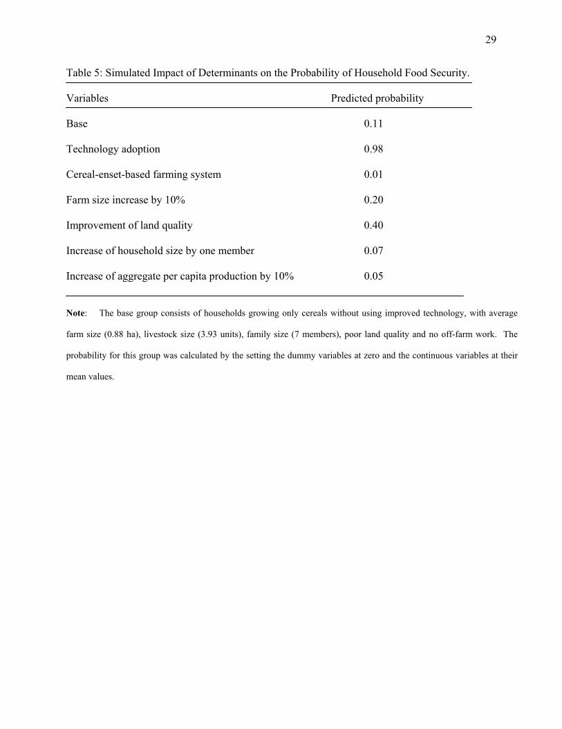
The level of probability due to changes in statistically significant determinants was also

computed in relation to a base group of households (Table 5). The base group consists of

households growing only cereals without using modern inputs, with average farm size (0.88 ha),

livestock size (3.93 tropical livestock unit), family size (7 persons), poor land quality, and no off-

farm income. The base group was selected by setting the dummy variables at zero and the

22

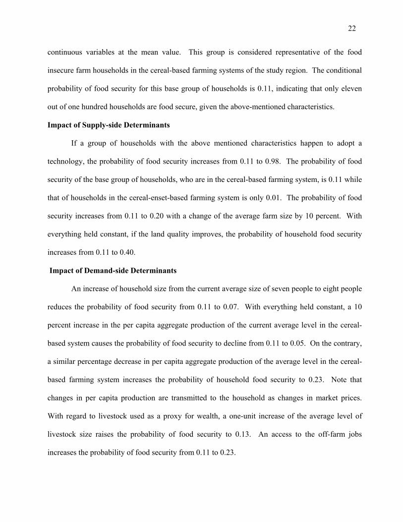
continuous variables at the mean value. This group is considered representative of the food

insecure farm households in the cereal-based farming systems of the study region. The conditional

probability of food security for this base group of households is 0.11, indicating that only eleven

out of one hundred households are food secure, given the above-mentioned characteristics.

Impact of Supply-side Determinants

If a group of households with the above mentioned characteristics happen to adopt a

technology, the probability of food security increases from 0.11 to 0.98. The probability of food

security of the base group of households, who are in the cereal-based farming system, is 0.11 while

that of households in the cereal-enset-based farming system is only 0.01. The probability of food

security increases from 0.11 to 0.20 with a change of the average farm size by 10 percent. With

everything held constant, if the land quality improves, the probability of household food security

increases from 0.11 to 0.40.

Impact of Demand-side Determinants

An increase of household size from the current average size of seven people to eight people

reduces the probability of food security from 0.11 to 0.07. With everything held constant, a 10

percent increase in the per capita aggregate production of the current average level in the cereal-

based system causes the probability of food security to decline from 0.11 to 0.05. On the contrary,

a similar percentage decrease in per capita aggregate production of the average level in the cereal-

based farming system increases the probability of household food security to 0.23. Note that

changes in per capita production are transmitted to the household as changes in market prices.

With regard to livestock used as a proxy for wealth, a one-unit increase of the average level of

livestock size raises the probability of food security to 0.13. An access to the off-farm jobs

increases the probability of food security from 0.11 to 0.23.

23

References

Alemu, K., Sandford, S., 1991. Enset in North Omo region. FRP Technical Pamphlet 1, Farm Africa, Addis Ababa, Ethiopia.

Amemya, T., 1981. Qualitative response models: A survey. Journal of Economic Literature, 29, 1483-1536.

Barnum, H., Squire, L., 1979. A model of an agricultural household: Theory and evidence. World Bank Occasional Papers 27, the Johns Hopkins University

Press, Baltimore and London. Brandt, S., Spring, A., Hiebsch, C., McCabe, T., Endale, T., Mulugeta, D., Gizachew,

W.M., Gebre, Y., Shigeta, M., Shiferaw, T., 1997. “The Tree against Hunger”, Enset-Based Agricultural Systems in Ethiopia, American Association for the Advancement of Science.

Cleaver, K., 1993. A strategy to develop agriculture in Sub-Saharan Africa and a focus for the World Bank, World Bank Technical Paper 203, Washington D.C.

Demaris, A., 1992. Logit modeling: Practical applications. International Educational and Professional Publisher, London.

FAO. 1998. Crop and food supply assessment mission to Ethiopia. FAO Global Information and Early Warning System on Food and Agriculture. World Food Program.

_____. 2001. Crop and food supply assessment mission to Ethiopia. FAO Global Information and Early Warning System on Food and Agriculture. World Food Program.

_____. 2002. Food crops and shortages in Ethiopia. Mimeo. Foster, P., 1992. The world food problem: Tackling the causes of undernutrition in the

third World, Lynne Rienner publishers, Boulder, Colorado. Gladwin, C., Thomson, A., Peterson, J., Anderson, A., 2000. Addressing food security in

Africa via multiple livelihoods strategies of woman farmers. Food Policy, 26, 177-207. Harsch, E., 1992. Enhanced food production: Food security in Africa: Priorities for

reducing hunger, Africa Recovery Briefing Paper 6, United Nations Department of Public Information, United Nations, New York.

Hiebsch, C., 1996. Yield of Enset ventricosum-a concept. In: Tsedeke, A., Hiebsch, H., Brandt, S., Siefu, G.M. (Eds.), Enset-based Agriculture in Ethiopia. Proceedings of the International Workshop on Enset, Institute of Agricultural Research, Addis Ababa, Ethiopia.

Huffnagel, H.P., 1961. Agriculture in Ethiopia, FAO, Rome. Kelsa, K., 1996. Soil problems associated with enset production. In: Tsedeke, A., Hiebsch,

H., Brandt, S., Siefu, G.M. (Eds.), Enset-based Agriculture in Ethiopia. Proceedings of the International Workshop on Enset, Institute of Agricultural Research, Addis Ababa, Ethiopia.

Markos, E., 1997. Demographic responses to ecological degradation and food insecurity in drought prone areas of northern Ethiopia. Thesis Publishers, Prinseneiland 305, 1013 LP Amsterdam, the Netherlands.

Maxwell, D., 1996. Measuring food insecurity: The frequency and severity of “coping strategies”. Food Policy, 21, 291-303.

Maxwell, S., 1996. Food security: A post-modern Perspective. Food Policy, 21, 155- 170.

Ministry of Economic Development and Cooperation (MEDAC), 2000. Poverty reduction strategy. Addis Ababa, Ethiopia. Mimeo.

Olmstead, J., 1974. The versatile enset plant: Its use in the Gamo highlands. Journal of

24

Ethiopian Studies 12(2), 147-153. Pankhurst, R., 1996. Social consequences of enset production. In: Tsedeke, A., Hiebsch,

H., Brandt, S., & Siefu, G.M. (Eds.), Enset-based Agriculture in Ethiopia. Proceedings of the International Workshop on Enset, Institute of Agricultural Research, Addis Ababa, Ethiopia.

Sen, A., 1981. Poverty and famines: An essay on entitlement and deprivation. Clarendon Press, Oxford. Shiferaw, T., Bizuayehu, H., 1995. Diagnostic survey of enset in Mareka district of

North Omo zone. Awassa Research Center, Awassa. Mimeo. Sijm, J.,1997. Food security and policy interventions in Sub-Saharan Africa. Thela

Publishers, Prinseneiland, Amsterdam, the Netherlands. Sisay, A., 1995. Perspectives on rural policy, rural poverty and food insecurity in Ethiopia.

In: Mulat, D., Wolday, A., Ehui, S., Tesfaye, Z. (Eds.), Food security, Nutrition, and poverty Alleviation in Ethiopia: Problems and Prospects. Proceedings of the Inaugural and First Annual Conference of the Agricultural Economics Society of Ethiopia, Addis Ababa, Ethiopia.

Smeds, H., 1955. The enset planting culture of Eastern Sidamo, Ethiopia. Strauss, J., 1983. Socioeconomic determinants of food consumption and production in

rural Sierra Leone: Application of an agricultural household model with several commodities. MSU International Development Papers. Department of Agricultural Economics, Michigan State University, East Lansing, Michigan.

Taye, B., 1996. An overview on enset research and future technological needs for enhancing its production and utilization. In: Tsedeke, A., Hiebsch, H., Brandt, S., Siefu, G.M. (Eds.), Enset-based Agriculture in Ethiopia. Proceedings of the International Workshop on Enset, Institute of Agricultural Research, Addis Ababa, Ethiopia.

Thomson, A.M., Metz, M., 1997. Implications of economic policy for food security. Training materials for agricultural planning. Agricultural Policy Support Service Agricultural Policy Division, Food, and Agricultural Organization, Rome.

Tomich, T.P., Kilby, P., Johnston, B.F., 1995. Transforming agrarian economies. Cornell University Press, Ithaca, N.Y.

Yotopoulos, P., 1983. A micro economic-demographic model of the agricultural household in the Philippines. FAO Economic and Social Development Paper, Rome, Italy.

Wolday, A., 1995. Ethiopia’s market liberalization in agriculture: Consequences and responses. In: Mulat, D., Wolday, A., Ehui, S., Tesfaye, Z. (Eds.), Food security, Nutrition and Poverty Alleviation in Ethiopia: Problems and Prospects. Proceedings of the Inaugural and First Annual Conference of the Agricultural Economics Society of Ethiopia, Addis Ababa, Ethiopia.

World Bank, 1986. Poverty and hunger: Issues and options for food security in developing countries. Washington D.C.

25

Indifference curve

Market possibility line

Transformation curve

Indifference curve

Market possibility line

Qj

Qi

Qi

P’

P

L L’ L

Q’i

Qi

Fi

Fj

Qj

Qi

Figure 1: Production and consumption decisions Figure 2: Decision on time between between two goods work and leisure Source: Adapted from Straus (1983)

26

Table 1: Household Food Security Rates by Selected Variables in Southern Ethiopia.

Variables Food Food Chi-square t-statistic insecure secure Technology adoption (%)

Non-adopters 60.6 39.4 27.86*** --- Adopters 26.8 73.2

Farming systems (%) Cereal-based 29.3 70.7 11.089*** --- Cereal-enset-based 50.0 50.0

Farm size (ha.) 0.54 1.13 --- -8.60***

Land quality (%) Poor 66.7 33.3 15.403*** --- Good 34.1 65.9

Household size (#) 8.0 7.0 --- 2.463**

Wealth (tlu.) 3.24 4.39 --- -3.795***

Access to off-farm work (%) No 41.4 58.6 2.856* --- Yes 24.0 76.0

Note: *** is statistically significant at P<0.01; ** is statistically significant at P<0.05; and * is statistically significant at P<0.1. tlu = tropical livestock unit.

Chi-square analysis is applied to the discrete variables to see if there is a systematic association between food

security and the respective discrete variables, while t-test is applied to the continuous variables to see if there is a

statistically significant difference between the food secure and insecure groups of households with regard to the

continuous variables, without controlling for the effect of other independent variables.

27

Table 2: Parameter Estimates of Household Food Security Model in Southern Ethiopia.

Variables Estimate Standard t-statistic p-value errors Constant 3.5955 2.3181 1.5511 0.1210 Technology adoption (X1) 5.8653 0.9511 6.1669 0.0000 Farming system (X2) -2.5055 0.8382 -2.9891 0.0280 Farm size (X3) 7.6178 1.1969 6.3646 0.0000 Land quality (X4) 1.6621 0.7711 2.1555 0.0311 Household size (X5) -0.5681 0.1187 -4.7860 0.0000 Per capita aggregate production (X6) -5.2422 1.2869 -4.0735 0.0000

Wealth (X7) 0.1986 0.1372 1.4475 0.1477

Off-farm (X8) 0.8397 0.8478 0.9883 0.3220

Access to market (X9) -0.0188 0.0099 1.8990 0.0571

Restricted log likelihood value [ ]=)(2 0LLog 629.332−

Unrestricted log likelihood value [ 254.113)](2 1 −=LLog

Log likelihood value ( [ ] )001.0(375.219))log(2()log(2) 10)9(2 <=−−−== PLLdfχ .

% of correct prediction = 89.5

28

Table 3: “Partial” effects for the Significant Continuous Determinants.

Determinants “Partial” effects

Farm size (ha.) 0.5401

Household size (#) -0.0403

Per capita aggregate production(kg.) -0.3717 Access to the market (minute) 0.0013

Note: The “partial” effects of the continuous individual variables on household food security are calculated using

jiiij

i

xβφφ

φ ˆ)ˆ1(ˆˆ

−=∂∂

.

Table 4: Change in probabilities between 0=iX and 1=iX for the Significant Discrete Determinants

Determinants Probabilities Change in Probabilities Technology adoption (%)

Non-adopters 0.3396 0.4332 Adopters 0.7728 Farming systems (%)

Cereal-based 0.7050 -0.1754 Cereal-enset-based 0.5296 Land quality (%)

Poor 0.4948 0.1226 Good 0.6174 Note: The change in probabilities of household food security due to the change in the significant discrete explanatory

variables were calculated by taking the difference of the mean probabilities estimated for the respective discrete variables,

Xi =0 and Xi =1.

29

Table 5: Simulated Impact of Determinants on the Probability of Household Food Security.

Variables Predicted probability

Base 0.11

Technology adoption 0.98

Cereal-enset-based farming system 0.01

Farm size increase by 10% 0.20

Improvement of land quality 0.40

Increase of household size by one member 0.07

Increase of aggregate per capita production by 10% 0.05

Note: The base group consists of households growing only cereals without using improved technology, with average

farm size (0.88 ha), livestock size (3.93 units), family size (7 members), poor land quality and no off-farm work. The

probability for this group was calculated by the setting the dummy variables at zero and the continuous variables at their

mean values.