Munich Personal RePEc Archive

Determinants and Potentials of Foreign

Trade in Ethiopia: A Gravity Model

Analysis

Yeshineh, Alekaw Kebede

2016

Online at https://mpra.ub.uni-muenchen.de/74509/

MPRA Paper No. 74509, posted 14 Oct 2016 13:19 UTC

Determinants and Potential of

Foreign Trade in Ethiopia: A Gravity

Model Analysis

By Alekaw Kebede Yeshineh

Research Analyst

Ethiopian Development Research Institute

Addis Ababa, Ethiopia

2014

i

Table of Contents 1. Introduction ........................................................................................................................................ 1

2. Overview of Ethiopian Merchandise Trade ........................................................................................ 4

2.1 Merchandise Trade Balance .......................................................................................................... 4

2.2 Merchandise Exports ................................................................................................................... 5

2.2.1 Composition of Exports .......................................................................................................... 6

1.2.2 Direction of Ethiopian Exports ............................................................................................... 7

2.3 Merchandise Imports .................................................................................................................... 9

2.3.1 Composition of Ethiopian Imports ......................................................................................... 9

23.2 Origins of Ethiopian Merchandise Imports ........................................................................... 11

3. Review of a Gravity Model of International Trade ......................................................................... 12

3.1 . Theoretical Review of the Gravity model ................................................................................. 12

3.2. Empirical Literature Survey ........................................................................................................ 14

4. Data Sources and Model Specifications ............................................................................................ 17

4.1 Data and Sample Size .................................................................................................................. 17

4.2. Methodology .............................................................................................................................. 18

4.2.1. The Fixed Effect Model (FEM) ............................................................................................. 18

4.2.2 Random Effect Model (REM) ............................................................................................... 18

4.2.3 The Hausman-Taylor (HT) approach. ................................................................................... 19

4.3. Model Specifications .................................................................................................................. 20

4.3.1 Augmented gravity model ................................................................................................... 20

4.3.2 Specification of the Gravity Model for Ethiopian Export ..................................................... 21

4.3.3 Specification of the Gravity Model for import ..................................................................... 21

4.3.4 Specification of the Gravity Model for the total trade (export plus import) ....................... 21

5. Estimation Results and Discussion .................................................................................................... 22

5.1 Estimation and Discussion of Export Model ............................................................................... 22

5.2 Estimation and Discussion of Import Model ............................................................................... 24

5.3 Estimation and Discussion of Total Trade Model ....................................................................... 25

5.4 ESTIMATING TRADE POTENTIAL ..................................................................................................... 27

5.4.1. Estimating Ethiopia’s Export potential.................................................................................... 27

5.5.2. Estimating Ethiopia’s Import Trade Potential ........................................................................ 29

5.5.3. Estimating Ethiopia’s Total Trade Potential ............................................................................ 31

ii

6. Conclusions and Recommendations ................................................................................................. 34

6.1 Conclusions ................................................................................................................................. 34

6.2 Recommendations ...................................................................................................................... 35

References ............................................................................................... Error! Bookmark not defined.

List of Tables

Tables Pages

Table 1:Export receipt at commodity level in million USD (2005 -2012) ............................................. 7

Table 2:Top 20 Export Destinations, FOB Value (Million USD) .......................................................... 8

Table 3:Import share by commodity classification ,% of total import(EDRI Classification) ............... 10

Table 4:Import payment growth rate by commodity classification ,(EDRI Classification) ................. 10

Table 5:Top 20 import partners of Ethiopian (shares %) ...................................................................... 11

Table 6:Export Model based on equation 7 .......................................................................................... 23

Table 7:Import Model based on equation 8 .......................................................................................... 25

Table 8:Total Trade Model based on equation 9 .................................................................................. 26

Table 9:Elasticities for the estimation of potential Export .................................................................... 27

Table 10:Ethiopian Export Trade Potential .......................................................................................... 29

Table 11:Elasticities for the estimation of potential Import .................................................................. 30

Table 12:Ethiopian Import Trade Potential .......................................................................................... 31

Table 13:Elasticities for the estimation of potential Import .................................................................. 32

Table 14:Total Merchandise Trade Potential ........................................................................................ 33

List of Figures

Figures Pages

Figure 1:Trend in Merchandise Statistics in Million USD (1998- 2012) 4

Figure 2:Trend in growth rate of merchandise trade(1999- 2012) 5

Figure 3:Export Receipts from Merchandise Trade in million USD (1998-2012) 6

Figure 4:Import cif Values in million USD (1998-2012) 9

iii

Abstract

In this study, attempts are made to provide a theoretical justification for using the gravity

model in analyzing the bilateral trade flows. The augmented gravity model was adopted to

analyse Ethiopia's trade with its main trading partners using the panel data estimation

technique. Estimations of the gravity model for export, import and total trade (sum of

exports and imports) are carried on. The estimated results show that Ethiopia's export, import

and total trade are positively determined by the size of the economies, per capita GDP

differential and openness of the trading countries' economies. Specifically, the major

determinants of Ethiopia’s exports are: size of the economies(GDP's of Ethiopia and that of

partner), partner countries’ openness of economies, economic similarity and per capita GDP

differential of the countries. All these factors affected Ethiopia's export positively except

similarity indicator. The exchange rate, on the other hand, has no effect on Ethiopia's export

trade. Ethiopia's imports are also determined by GDP's (of Ethiopia and the partner country),

per capita income differentials and openness of the countries involved in trade.

Transportation cost is found to be a significant factor in influencing Ethiopia's trade

negatively. On the other hand, Ethiopia's export and import trade are not found to be

influenced to by common border . The country specific effects show that Ethiopia could do

better by trading more with Comesa member countries and newly emerging economies of

Asia such as Hong Kong, Singapore and Yemen as well as European countries like Turkey

and Russia.

Key Words: Gravity Model, Panel Data, Fixed Effect Model, Random Effect Model,

Hausman Tyalor Model, Ethiopia’s Trade.

1

1. Introduction

The performance of foreign trade in Ethiopia has increased significantly in recent times.

Available evidences shows that the value of both exports and imports improved tremendously

since the implementation of the Plan for Accelerated and Sustained Development to End

Poverty (PASDEP) in 2004/05.The Government has implemented many export incentive

packages besides the reduction of tariff rate for import of raw materials and capital goods to

the manufacturing sector. Nevertheless, according to the data of Ethiopian Revenue and

Customs Authority (ERCA), during the period 2004 to 2012, the value of the country’s

export increased from USD 615.26 million to USD 2,772.12 million, while import rose from

USD 3,040.84 to 11,556.14 million over the same period. As a result the fast growth of

import compared to export, trade deficit of the country increased from USD 2,425.58 million

to 8,784.02 million over the period. This merchandise trade deficit divergence has resulted to

wider current account deficit in the country.

The trade deficit and its economic and social implications are matters of concern to both the

public and private sectors. Thus, it is important for both parties to work together with respect

to the contents and marketing strategies of export items. There is an urgent need to address

the trade deficit not only from export side but also from the expenditure or import side by

identifying products that can be locally produced to reduce foreign exchange out flows. At

the same time, expanding the volume of trade and diversifying of export products and market

destinations need to be investigated in detail to narrow the deficit.

As a matter of fact the export basket of the country is concentrated on few agricultural

products such as coffee, oilseeds, pulses and semi processed leather. The export destination

of the country's products are very limited as well. On the other hand, as a consequence of the

grow of the domestic economy, the demand for consumer and capital goods as well as

various other services is growing. Given such circumstances, the fiscal and non fiscal

incentives will not be effective enough to bring solution for narrowing the trade deficit. It is

rather important to supplement such incentives by other measures that give special priority

for boosting export trade such as diversifying export baskets and destinations besides

promoting import substituting projects. Firms relying on imported inputs and capital goods

have been blaming the customs and logistics inefficiency as they are affected by delays in

importing essential materials or/and machinery as well as the impossibility of importing

2

them altogether. Furthermore, the foreign exchange controls and procedures which have been

established by the government in response to the shortage of foreign currency caused

additional costs and delays for all firms in Ethiopia as it affected their dealing with foreign

trade partners.

According to the Ministry of Foreign Affairs Foreign Trade Promotion Manual (MOF,2007)

Ethiopia's foreign trade policy has three general objectives. The first is developing and

ensuring broad international market for the country's agricultural products and the second one

is generating sufficient foreign exchange which is essential for importing capital goods,

intermediate inputs and other goods and services that are necessary for the growth and

development of the economy. The third one is improving the efficiency and international

competitiveness of domestic producers through participation in the international market. The

core assumption of the country’s Industrial Development Strategy (IDS) of 2002 was also

the primacy of the free market, and government support is only to be provided on a

temporary basis in order to help domestic industry become internationally competitive. In

line with the overarching Agricultural Development Led Industrialization (ADLI) strategy the

IDS focuses on labour intensive industrial inputs and consumption goods for agriculture and

value added/processed goods, especially for exports. Although the IDS has undoubtedly

contributed to Ethiopia’s increasing exports, it is now clear that the export-led strategy must

be complemented by other measures that help to address the widening trade deficit.

Product diversification that aims at moving away from a limited basket of exports in order to

mitigate the economic risks of dependence upon few commodity exports is imperative. As

export is concentrated in a few commodities, there has been serious short-run and long-run

economic risks being experienced in Ethiopia. The short term economic risks are felt to the

economy through volatility and instability of foreign exchange earning which could have

adverse macroeconomic effects on growth, employment, investment planning, import and

export capacity, foreign exchange cash flow, inflation, capital flight and undersupply of

investments by risk averse investors and others. In the long term, secular and unpredictable

declining terms of trade trends may exacerbate short run effects. Reducing dependence upon

limited number of geographical destinations for the export sales can also be another way of

reducing ,if not avoiding, the economic risks of less diversification.

3

Ethiopia is located in a strategically important place to the Asia and Europe markets with rich

agro ecological zones suitable to fresh and organic agricultural products. Furthermore, the

country has been given many special trade preferential arrangements such as AGOA in the

United States Market and Everything but Arms(EBA) as well as Economic Partnership

Agreement(EPA) with the European Union. Despite all these opportunities, the export

performance of the country is below satisfactory. Dealing with the underperformance and

constraints of the external trade sector especially the export sector is critical in to exploit

country's trade potential and use the trophy of trade to the entire economy.

The trade potential is exploited when the maximum possible trade that could occur between

any two countries that liberalized trade restrictions. It refers to the situation of trade in free

trade with no restrictions that constitute optimum trade frontier. It predicts the trade that

could be possible given the current level of trade, transport and institutional technologies. In

other words, it is the maximum level of trade given the current level of determinants of trade

as well as the least level of restrictions within the economic system. Given the potential gains

o f trade, countries are interested to liberalize their economies to enjoy the benefits of trade and

globalization through bilateral and multilateral process. It is important that each country may

know its full trade potential with other countries or other regions in order to get the engagement

process started.

The increasing volume and value of trade performance requires good trade policies based on

reliable information. In this regard, although there have been some studies on trade issues of

the country, they are not updated and some of them couldn’t explain the major factors of

trade in Ethiopia. In this paper investigation on the major determinants of trade (export,

import and total trade) will have been made. Furthermore, the study is devoted to compute

the trade potential based on the estimated augmented gravity model.

The organization of the paper is as follows. Section 2 provides a brief overview of the

Ethiopia’s bilateral trade flows. Section 3 deals with a brief review of related literature that

existed in estimating potential trade in empirical research by using gravity equation analysis

of trade. Furthermore, section 4 presents the data and the suggested methodology of gravity

equation while results from the estimation are discussed in the section 5. Lastly, section 6

contains the overall conclusions and recommendations of this study.

4

2. Overview of Ethiopian Merchandise Trade

2.1 Merchandise Trade Balance

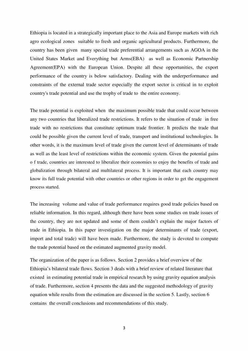
The merchandise trade deficit continued to widen since 2002 as shown below in Figure1.

The deficit in 2012 increased to 30.08 per cent relative to that of 2011 (it increased from

$6,753.04 million to $8,784.02 million). The deficit has exerted an upward pressure since

2006. The upward pressure of the deficit has reached to its peak and became more

recognizable in 2012 after fall in 2009 and 2010.

Figure 1:Trend in Merchandise Statistics in Million USD (1998- 2012)

0.00

2,000.00

4,000.00

6,000.00

8,000.00

10,000.00

12,000.00

14,000.00

1998 1999 2000 2001 2002 2003 2004 2005 2006 2007 2008 2009 2010 2011

FOB_MUSD CIF_MUSD Deficit

Source: ARCA and Petroleum Enterprise

The year on year merchandise trade deficit was about 61.31 percent of the total merchandise

trade in 2012 while it was about 13 percent in 2011. The capacity of export to finance

merchandise import trade has been less than 30 percent of the total merchandise import

payments over the last several years. It was only 24 percent of the import payment that could

be financed by the export receipt during these years. The ratio of export revenue to import

expenditure on merchandise trade reached at its lowest point in 2008 and the 2012 export-

import ratio has been the third lower ratio in the last ten years profile of merchandise trade

since 2005.

5

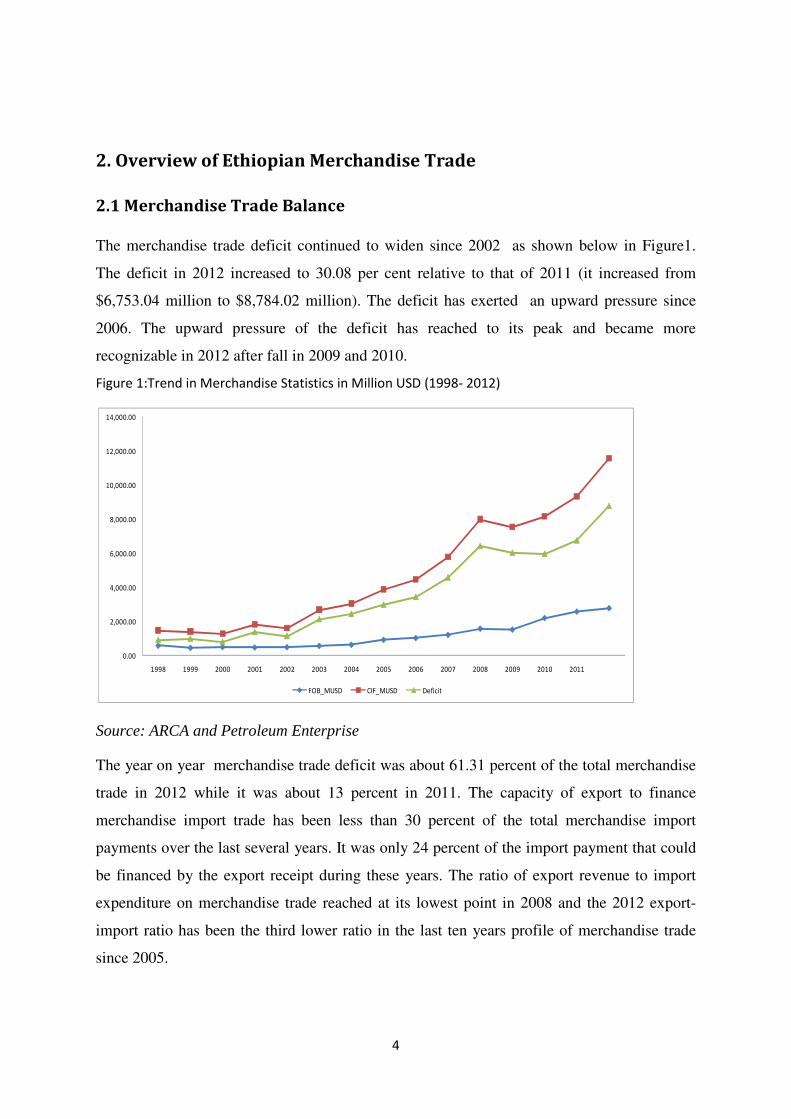
Figure 2:Trend in growth rate of merchandise trade(1999- 2012)

Source: ERCA and Petroleum enterprise

As shown in the above figure, the growth rate of merchandise trade deficit was less than that

of export and import during the period of 2009 through 2011. During this period, the growth

rate of export exceeded the growth rate of import. However in 2012 deficit has over took

both export and import and it became the second largest deficit registered next to that of the

deficit in 2008 over the last five years. This widened merchandise trade deficit is used to be

the result of increased import expenditure mainly on capital goods and other consumer goods

following the growth of the national economy. On the one hand, relatively less diversified

export receipt could not be able to adequately respond in covering the growing import

demand. Particularly the huge public investment being carried in the country has contributed

a lot for the divergence of the import payments and export receipts. This caused import

expenditure to grow by about 23.93 percent in 2012 while the export receipt grew only by

about 7.8 per cent in the same year.

2.2 Merchandise Exports

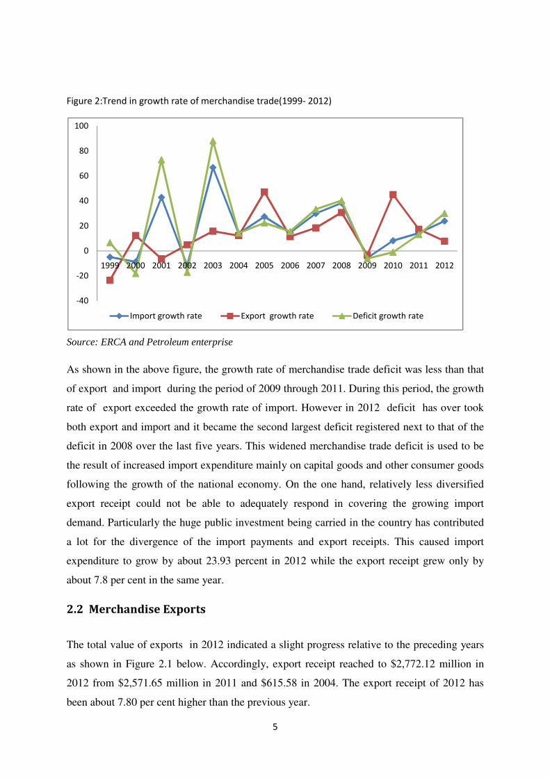
The total value of exports in 2012 indicated a slight progress relative to the preceding years

as shown in Figure 2.1 below. Accordingly, export receipt reached to $2,772.12 million in

2012 from $2,571.65 million in 2011 and $615.58 in 2004. The export receipt of 2012 has

been about 7.80 per cent higher than the previous year.

1999 2000 2001 2002 2003 2004 2005 2006 2007 2008 2009 2010 2011 2012

-40

-20

0

20

40

60

80

100

Import growth rate Export growth rate Deficit growth rate

6

Figure 3:Export Receipts from Merchandise Trade in million USD (1998-2012)

560.66429.37 482.09 451.49 473.47

548.19 615.26

905.581,009.22

1,194.99

1,562.811,510.34

2,191.34

2,571.65

2,772.12

0.00

500.00

1,000.00

1,500.00

2,000.00

2,500.00

3,000.00

1998 1999 2000 2001 2002 2003 2004 2005 2006 2007 2008 2009 2010 2011 2012

FOB_MUSD

Source: ERCA

Comparison of FOB values with previous years revealed that there has been an impressive

growth in the export performance especially since 2010 as shown in figure 2.1 above.

However, the receipt has been highly dependent on agricultural raw materials whose price

grows much lower than that of finished industrial goods.

2.2.1 Composition of Exports

The increase in export receipts in recent years was attributed to progresses in both prices and

volumes of all commodities mainly the export of coffee, oilseeds, pulses, chat and gold. The

increase in receipts from these export items moved up the overall export receipt of the year.

The export revenue from coffee was remarkable and it has continued to be the major and

reliable export crop of the country over the last previous years.

Generally, the fact that Ethiopia’s export is mainly dependent on few primary commodities

has worsened the vulnerability of receipt instability from merchandise export. The export

receipt from five commodities, namely coffee, oilseeds, Pulses, Chat and Live Animals has

accounted the lion share that any effect on these dominant commodities' price could

adversely affect the entire external trade balance.

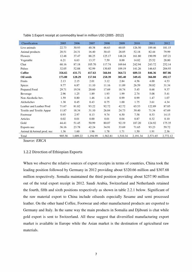
7

Table 1:Export receipt at commodity level in million USD (2005 -2012)

Classification 2005 2006 2007 2008 2009 2010 2011 2012

Live animals 22.73 30.93 40.38 46.63 60.05 126.50 189.46 181.15

Animal products 20.51 24.31 16.40 30.43 28.05 52.18 82.44 79.99

Flowers 12.48 37.47 88.25 125.17 148.24 161.80 190.99 187.21

Vegetable 6.21 6.63 13.37 7.59 8.00 14.82 25.52 28.80

Chat 68.16 87.18 105.70 117.74 169.64 242.94 243.72 252.14

Pulses 32.05 52.88 92.99 130.85 109.19 141.26 146.63 204.93

Coffee 356.65 431.75 417.63 566.04 364.72 689.33 846.36 887.86 Oil seeds 175.80 128.29 157.04 258.39 385.40 349.45 366.80 492.17 Fruits 2.13 2.15 2.01 3.12 2.84 4.56 4.00 4.53

Spices 9.77 6.87 11.10 11.16 11.89 26.59 38.82 31.34

Prepared Food 29.71 19.54 20.60 17.69 18.74 5.45 8.68 9.37

Beverage 2.96 1.25 1.89 1.93 1.99 2.74 5.08 5.41

Non Alcoholic bev. 1.59 0.80 1.46 1.18 0.99 0.99 1.47 1.07

Alcholicbev 1.38 0.45 0.43 0.75 1.00 1.75 3.61 4.34

Leather and Leather Prod 71.67 81.82 93.22 92.72 42.72 65.53 122.89 87.85

Textile and Textile Appar 11.87 18.34 31.10 26.84 24.73 39.40 71.34 67.69

Footwear 0.93 2.97 8.13 9.74 6.50 7.58 8.53 14.15

Articles 0.02 0.01 0.00 0.01 0.04 0.87 0.32 0.10

Gold 44.41 51.45 50.99 80.07 92.19 187.20 124.92 175.35

Exports nec 36.16 23.78 42.24 34.91 33.69 71.65 93.23 59.72

Animal &Animal prod. nec 1.36 1.60 1.96 1.78 1.71 1.50 1.91 2.36

Total 905.58 1,009.22 1,194.99 1,562.81 1,510.34 2,191.34 2,571.65 2,772.12

Source: ERCA

1.2.2 Direction of Ethiopian Exports

When we observe the relative sources of export receipts in terms of countries, China took the

leading position followed by Germany in 2012 providing about $320.66 million and $307.68

million respectively. Somalia maintained the third position providing about $257.90 million

out of the total export receipt in 2012. Saudi Arabia, Switzerland and Netherlands retained

the fourth, fifth and sixth positions respectively as shown in table 2.2.1 below. Significant of

the raw material export to China include oilseeds especially Sesame and semi processed

leather. On the other hand Coffee, Footwear and other manufactured products are exported to

Germany and Italy. In the same way the main products in Somalia and Djibouti is chat while

gold export is sent to Switzerland. All these suggest that diversified manufacturing export

market is available in Europe while the Asian market is the destination of agricultural raw

materials.

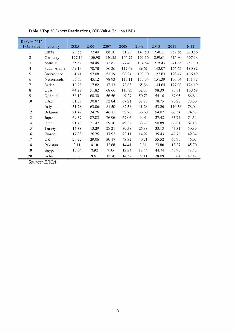
8

Table 2:Top 20 Export Destinations, FOB Value (Million USD)

Rank in 2012 FOB value country 2005 2006 2007 2008 2009 2010 2011 2012

1 China 79.68 72.40 68.20 81.22 149.80 238.11 282.66 320.66

2 Germany 127.14 130.90 120.85 166.72 106.16 259.61 315.80 307.68

3 Somalia 35.37 54.48 72.81 77.40 114.64 215.43 241.38 257.90

4 Saudi Arabia 59.18 70.78 86.36 122.49 89.67 143.07 166.63 190.92

5 Switzerland 61.41 57.08 57.79 98.24 100.70 127.83 129.47 176.49

6 Netherlands 35.53 45.12 78.93 118.11 113.34 151.39 180.34 171.47

7 Sudan 10.98 17.82 47.13 72.83 65.86 144.64 177.08 124.19

8 USA 44.29 51.82 68.66 113.73 52.55 98.39 95.81 108.69

9 Djibouti 58.13 60.30 56.56 49.29 50.73 54.16 69.05 86.84

10 UAE 31.09 30.87 32.84 67.21 57.75 78.75 76.28 78.30

11 Italy 51.78 63.06 81.50 82.58 41.28 53.20 110.58 78.04

12 Belgium 21.42 34.76 46.11 52.76 36.60 54.07 68.54 74.58

13 Japan 69.37 87.83 76.96 62.07 9.06 37.48 35.74 74.54

14 Israel 21.40 21.47 29.70 49.39 38.72 50.89 66.81 67.18

15 Turkey 14.38 13.29 28.21 39.58 26.33 33.13 45.31 50.39

16 France 17.38 26.76 17.92 23.11 14.97 35.43 49.76 49.34

17 UK 29.22 29.06 30.17 43.32 49.71 55.52 66.70 46.97

18 Pakistan 3.11 8.10 12.68 14.41 7.81 23.80 13.37 45.70

19 Egypt 16.04 8.92 7.35 13.34 13.44 44.74 45.90 43.45

20 India 8.08 9.61 15.70 14.59 22.11 28.09 33.64 42.42

Source: ERCA

9

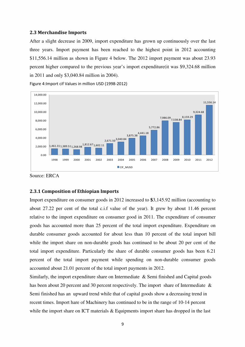
2.3 Merchandise Imports

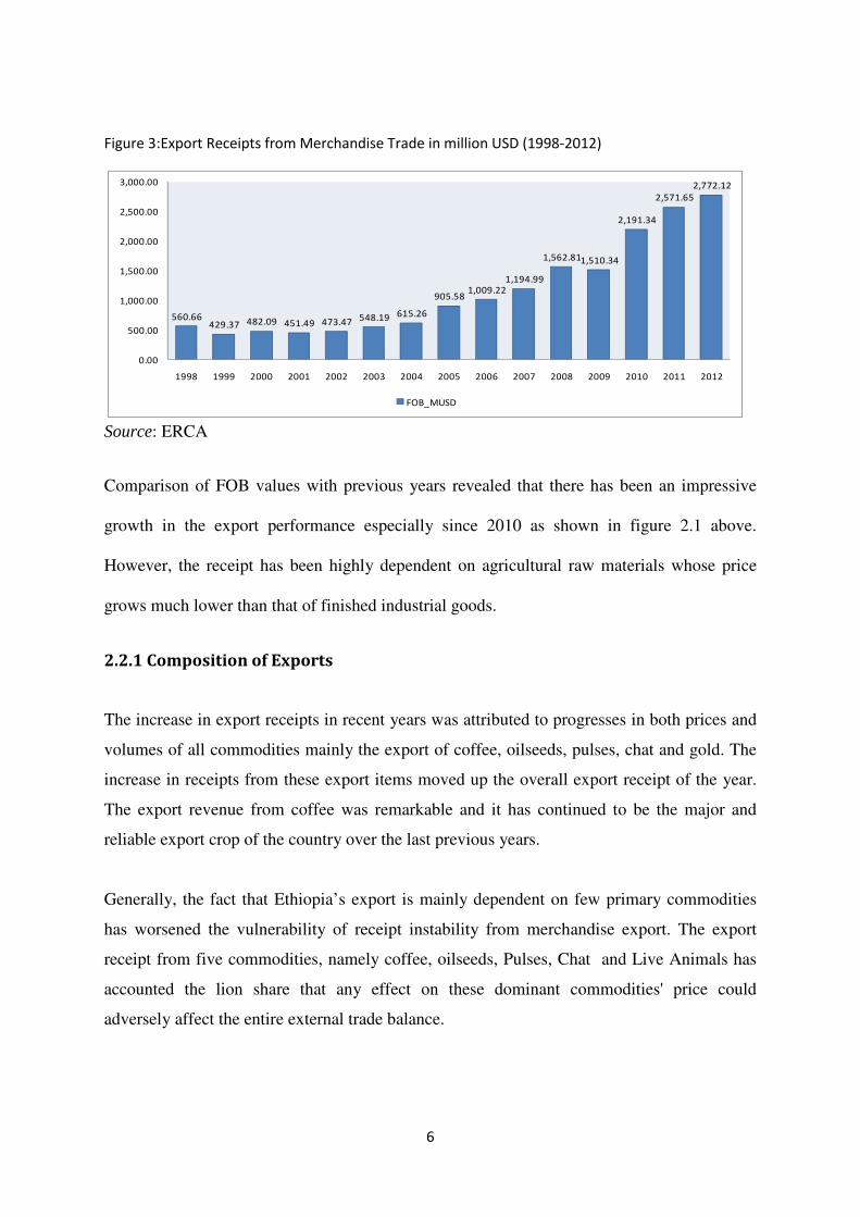
After a slight decrease in 2009, import expenditure has grown up continuously over the last

three years. Import payment has been reached to the highest point in 2012 accounting

$11,556.14 million as shown in Figure 4 below. The 2012 import payment was about 23.93

percent higher compared to the previous year’s import expenditure(it was $9,324.68 million

in 2011 and only $3,040.84 million in 2004).

Figure 4:Import cif Values in million USD (1998-2012)

1,461.311,389.511,268.981,812.671,602.11

2,671.503,040.84

3,875.384,441.18

5,772.86

7,986.097,538.84

8,159.29

9,324.68

11,556.14

0.00

2,000.00

4,000.00

6,000.00

8,000.00

10,000.00

12,000.00

14,000.00

1998 1999 2000 2001 2002 2003 2004 2005 2006 2007 2008 2009 2010 2011 2012

CIF_MUSD

Source: ERCA

2.3.1 Composition of Ethiopian Imports

Import expenditure on consumer goods in 2012 increased to $3,145.92 million (accounting to

about 27.22 per cent of the total c.i.f value of the year). It grew by about 11.46 percent

relative to the import expenditure on consumer good in 2011. The expenditure of consumer

goods has accounted more than 25 percent of the total import expenditure. Expenditure on

durable consumer goods accounted for about less than 10 percent of the total import bill

while the import share on non-durable goods has continued to be about 20 per cent of the

total import expenditure. Particularly the share of durable consumer goods has been 6.21

percent of the total import payment while spending on non-durable consumer goods

accounted about 21.01 percent of the total import payments in 2012.

Similarly, the import expenditure share on Intermediate & Semi finished and Capital goods

has been about 20 percent and 30 percent respectively. The import share of Intermediate &

Semi finished has an upward trend while that of capital goods show a decreasing trend in

recent times. Import hare of Machinery has continued to be in the range of 10-14 percent

while the import share on ICT materials & Equipments import share has dropped in the last

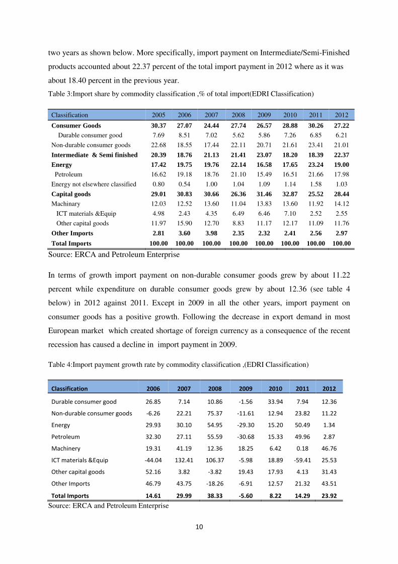
10

two years as shown below. More specifically, import payment on Intermediate/Semi-Finished

products accounted about 22.37 percent of the total import payment in 2012 where as it was

about 18.40 percent in the previous year.

Table 3:Import share by commodity classification ,% of total import(EDRI Classification)

Classification 2005 2006 2007 2008 2009 2010 2011 2012

Consumer Goods 30.37 27.07 24.44 27.74 26.57 28.88 30.26 27.22 Durable consumer good 7.69 8.51 7.02 5.62 5.86 7.26 6.85 6.21

Non-durable consumer goods 22.68 18.55 17.44 22.11 20.71 21.61 23.41 21.01

Intermediate & Semi finished 20.39 18.76 21.13 21.41 23.07 18.20 18.39 22.37

Energy 17.42 19.75 19.76 22.14 16.58 17.65 23.24 19.00

Petroleum 16.62 19.18 18.76 21.10 15.49 16.51 21.66 17.98

Energy not elsewhere classified 0.80 0.54 1.00 1.04 1.09 1.14 1.58 1.03

Capital goods 29.01 30.83 30.66 26.36 31.46 32.87 25.52 28.44

Machinary 12.03 12.52 13.60 11.04 13.83 13.60 11.92 14.12

ICT materials &Equip 4.98 2.43 4.35 6.49 6.46 7.10 2.52 2.55

Other capital goods 11.97 15.90 12.70 8.83 11.17 12.17 11.09 11.76

Other Imports 2.81 3.60 3.98 2.35 2.32 2.41 2.56 2.97

Total Imports 100.00 100.00 100.00 100.00 100.00 100.00 100.00 100.00

Source: ERCA and Petroleum Enterprise

In terms of growth import payment on non-durable consumer goods grew by about 11.22

percent while expenditure on durable consumer goods grew by about 12.36 (see table 4

below) in 2012 against 2011. Except in 2009 in all the other years, import payment on

consumer goods has a positive growth. Following the decrease in export demand in most

European market which created shortage of foreign currency as a consequence of the recent

recession has caused a decline in import payment in 2009.

Table 4:Import payment growth rate by commodity classification ,(EDRI Classification)

Classification 2006 2007 2008 2009 2010 2011 2012

Durable consumer good 26.85 7.14 10.86 -1.56 33.94 7.94 12.36

Non-durable consumer goods -6.26 22.21 75.37 -11.61 12.94 23.82 11.22

Energy 29.93 30.10 54.95 -29.30 15.20 50.49 1.34

Petroleum 32.30 27.11 55.59 -30.68 15.33 49.96 2.87

Machinery 19.31 41.19 12.36 18.25 6.42 0.18 46.76

ICT materials &Equip -44.04 132.41 106.37 -5.98 18.89 -59.41 25.53

Other capital goods 52.16 3.82 -3.82 19.43 17.93 4.13 31.43

Other Imports 46.79 43.75 -18.26 -6.91 12.57 21.32 43.51

Total Imports 14.61 29.99 38.33 -5.60 8.22 14.29 23.92

Source: ERCA and Petroleum Enterprise

11

Import payment bill on energy in 2012 increased marginally by about 1.34 per cent against

the prior year which might be partly due to a fall in price of petroleum in the international

market over the last two years. Consequently, its share over the total import expenditure

dropped down to 19.00 per cent in the 2012 from 23.24 per cent in 2011 of the total import

payment. As a result, the import payments of the country in 2012 increased by about 23.93

per cent against the previous year.

23.2 Origins of Ethiopian Merchandise Imports

More than 20 percent of the import payment on merchandise goods in 2012 was originating

from China followed by Saudi Arabia and India accounting about 14 per cent and 9 per cent

of the total imports expenditure respectively. Kuwait and Turkey were the fourth and fifth

largest merchandise import originating markets in 2012. Germany, the leading source for

Ethiopian export receipt, supplied less than 2 per cent of the import demand of Ethiopian

economy in 2012. The top 20 import trading partners accounted for the import expenditure of

more than 90 percent (see table 5 below).

Table 5:Top 20 import partners of Ethiopian (shares %)

Rank in 2012 cif value Country 2005 2006 2007 2008 2009 2010 2011 2012

1 China 14.5 14.92 19.77 20.45 23.87 23.82 19.01 20.5

2 Saudi Arabia 15.49 20.27 12.21 14.86 12.21 12.17 10.17 13.93

3 India 6.57 6.9 7.82 7.69 8.27 7.4 8.76 9.16

4 Kuwait 0.04 0.04 0.09 0.07 0.04 0.04 2.51 6.05

5 Turkey 3.23 2.24 2.73 1.97 3.36 2.73 3.97 4.22

6 Italy 5.07 7.59 7.41 5.58 5.09 4.4 3.95 4.18

7 Japan 6.14 7.5 6.81 4.12 4.04 5.27 4.85 3.72

8 Ukraine 2.08 1.39 1.32 1.72 1.22 1.03 1.6 3.04

9 USA 10.94 3.78 4.86 4.41 5.66 5.45 4.81 2.97

10 Indonesia 1.98 1.87 1.22 1.19 1.11 1.04 2.14 2.93

11 UAE 1.15 1.1 2.92 8.71 4.06 5.92 5.45 2.44

12 France 1.6 2.14 1.61 1.56 1.34 1.19 1.59 1.78

13 S.Korea 1.58 1.62 1.87 1.3 1.64 1.1 1.81 1.72

14 Morocco 0.02 0.03 0.02 0.2 0.3 1.07 0.35 1.68

15 Malaysia 1.03 1.15 1.57 2.47 2.83 2.75 3.11 1.59

16 Germany 3.15 2.95 3.21 2.81 2.31 2.36 2.03 1.57

17 Thailand 0.93 1 1.32 0.89 0.98 1.49 1.48 1.4

18 Belgium 1.33 1.31 1.3 0.82 0.66 1.04 0.98 1.26

19 Russian 0.66 1.56 0.66 1.27 2.28 1.17 3.05 1.23

20 Brazil 1.24 1.71 2.02 0.54 1.06 1.49 0.87 1.19

Source: ERCA

12

3. Review of a Gravity Model of International Trade

3.1 . Theoretical Review of the Gravity model

The gravity model of international trade was originated from Newtonian law of universal

gravitation. The model has been successfully applied to study flows of various types such as

migration, foreign direct investment and more specifically to international trade flows. This

law in mechanics states that two bodies attract each other proportionally to the product of

each body’s mass divided by the square of the distance between their respective centres of

gravity . The gravity model for trade is analogous to this law. The analogy is as follows: the

trade flow between two countries is proportional to the product of each country’s ‘economic

mass’, measured their by GDPs (national incomes) and inversely proportional to the distance

between the countries’ respective ‘economic centres of gravity’, mostly their capitals.

Timbergen (1962) and Pöyhönen (1963) were the first authors applying the gravity equation

to analyse international trade flows. Since then, the gravity model has become a popular

instrument in empirical foreign trade analysis.

The gravity model can be expressed mathematically as : 1 2

3

i jij

ij

Y YT k

D

β β

β= -------------------------------------------------(1)

where Tij is the value of bilateral trade between country of origin and destination j, the Yi Yj

are country i’s and country j’s GDP. The variable Dij denotes the geographical distance

between countries’ capitals, k is the constant of proportionality and the 'sβ are response

parameters. For the sake of simplicity, equation (1) could be transformed to a log linear form

as follows:

0 1 2 3ln ln ln lnij i j ijT Y Y Dβ β β β= + + + ------------------------------------------(2)

where the 'sβ are the coefficients to be estimated. Equation (2) is the baseline model where

bilateral trade flows are expected to be a positive function of incomes and negative function

of distance. However, because of the existence of huge amount of variations in trade that

cannot be explained by the traditional variables, the basic gravity model has later been

augmented with many choice variables. Some models have generally been assumed to

comprise supply and demand factors (GDPs and populations), as well as trade resistance and

trade preference factors. Batra (2004) in the study of trade potential included additional

variables to control for differences in geographic factors, historical ties and economic factors

like the overall trade policy and exchange rate risk.

13

Assuming that we wish to test for N distinct effects, the gravity model can be written as:

0 1 2 31

ln ln ln lnN

ij i j ij s ss

T Y Y D Gβ β β β λ=

= + + + +∑ ------------------------------(3)

However, one should still underline that gravity equations perform a pretty well job at

explaining trade with just the size of economies and their distances. Distance is a proxy for

various factors that can influence trade such as transportation costs, time elapsed during

shipment, synchronization costs, communication costs, transaction costs or cultural distance

(Head, 2003)

Theoretical support of the research in this field was originally very poor, but since the

second half of the 1970s several theoretical developments have appeared in support of

the gravity model. Anderson (1979) was, perhaps, the first to give the gravity model a

theoretical legitimacy. He derived the gravity equation from expenditure systems where

goods are differentiated by origin (Armington preferences) and all transport costs are proxied

by distance. That is, he made the first formal attempt to derive the gravity equation from a

model that assumed product differentiation.

While Anderson’s analysis is at the aggregate level, Bergstrand (1985, 1989) develops a

microeconomic foundation to the gravity model. He stated that a gravity model is a reduced

form of the equation of a general equilibrium of demand and supply systems. In such a model

the equation of trade demand for each country is derived by maximizing a constant elasticity

of substitution (CES) utility function subject to income constraints in importing countries. On

the other hand, the equation of trade supply is derived from the firm’s profit maximization

procedure in the exporting country, with resource allocation determined by the constant

elasticity of transformation (CET). The gravity model of trade flows, proxied by value, is

then obtained under market equilibrium conditions, where demand for and supply of trade

flows are equal.

Eaton and Kortum (1997) also derived the gravity equation from a Ricardian framework,

while Helman(1987) derived it from an imperfect competition model. Helman and Krugman

(1985) used a differentiated product framework with increasing returns to scale to justify the

gravity model. More recently Deardorff (1995) derived it from the Heckscher-Ohlin model

which confirmed that the gravity equation characterises many models and can be justified

from standard trade theories.

Trade theories just explain why countries trade each other in different products but do not

explain why some countries’ trade volumes are more than others and why the level of trade

14

between countries tends to vary over time. This is the limitation of trade theories in

explaining the size of trade flows. Though traditional trade theories cannot explain the extent

of trade, the gravity model however, is successful in this regard. It allows more factors to be

taken into account to explain the extent of trade as an aspect of international trade flows (Paas

2002).

Therefore, the gravity model is an internationally accepted and useful tool to investigate

bilateral trade patterns and flows. Furthermore it can be used to test hypotheses about the

impact of specific policies as well as geographical or cultural circumstances on the bilateral

trade between trading partners.

3.2. Empirical Literature Survey

There are wide ranges of applied research where the gravity model is used to examine the

bilateral trade patterns and trade relationships. These studies use the gravity model both for

the aggregate bilateral trade and for product level trade. Both the cross -section and panel

data approaches have been used by these studies.

Many of these works have tried to examine the trade potential, trade determinants, trade

direction and trade enhancing impacts. Rahman(2003) for instance, examined the

determinants of Bangladesh trade using panel data estimation technique and generalised

gravity model. The author considers both economic and natural factors when estimating the

gravity model. The study covers data of 35 countries for 28 years (1972-99). Batra (2006)

considered augmented gravity model to estimate India’s trade potential. The model is based

on cross-section data of 2000. In a sample of 76 countries, Kalbasi (2001) examines the

volume and direction of trade for Iran dividing the countries into developing and industrial

countries. On this study the impact of the stage of development on bilateral trade is analysed.

Using cross-section and panel data Frankel (1997) also applied the gravity model to examine

roles of trading blocs, currency links, etc. Analysing the bilateral trade patterns worldwide

Frankel and Wei (1993) examined the impact of currency blocs and exchange rate stability on

trade. Anderson and Wincoop (2003) and Feenstra (2003) analyse the impact of multilateral

factors on bilateral trade flows using the gravity model.

Rahman and Ara (2010) employed a dynamic gravity approach to estimate foreign trade

potential for Bangladesh. The study was conducted based on bilateral trade flows between

Bangladesh and its eighty major trading partners. For the purpose of estimating the gravity

15

model, a static panel dataset (1995–2007) with random effects was used. Estimation results

reveal that economic size, distance, regional trade agreement and adjacency are among

significant variables of the model. Having predicted the natural trade flows with an in-sample

strategy, Rahman and Ara (2010) have identified partners with which Bangladesh has

unexploited trade potential. Accordingly, the magnitude of Bangladesh trade potential was

found very high with China, Japan, India, United States, Germany and Russia respectively.

Alemayehu (2009) examined the nature of the potential for intra-Africa trade and hence the

prospects for advancing regional economic integration. His study used the gravity model on

the panel data frame work. The model was estimated using a panel data of African countries

and their major trade partners around the world (2000− 2006). The estimated coefficients of

the model were used to simulate the potential for intra-Africa trade. The findings of his study

notified the existence of a potential for intra-Africa trade (about 63% weighted average for

Central and Western Africa region, and some 60% for Eastern and Southern Africa region).

More recently, Africa-China trade potential was assessed by Matias (2010), by applying a

combination of methodologies—stochastic frontier gravity approach and trade

complementarity index. For the former case, the study utilized a panel data of Chinese

exports to the African countries over the period 2001–2008. Matias (2010) estimated using a

stochastic gravity model, incorporating random disturbance and inefficiency terms. The

estimated model was then used to calculate trade efficiency and potential of China with 52

African countries. Accordingly, China has realized on average only 13% of its export

potential with African countries. Seychelles, Sao Tome and Principe, Comoros, Central

Africa Republic, Chad and Equatorial Guinea are partners with which China had the lowest

trade efficiency (high export potential).

Using a gravity framework Mulugeta (2009) investigated the determinants of Ethiopia's

export and import flows. Based on the panel dataset of major trade partners, estimation was

done with fixed effects model. The finding was that income and distance variables,

infrastructure as well as institutional qualities were among the basic determinants. Hussein

(2008) analyzed the impact of COMESA membership and other factors on the flow of

Ethiopia's exports. The study takes in to account the flow of annual exports to twenty

destinations over the period 1981–2006. He used a Tobit specification with random effects to

estimate the gravity model. Estimation results demonstrate that most traditional variables are

significant, while the impact of COMESA membership to create or divert exports was

16

negligible. The latter finding seems consistent with what Alemayehu and Haile (2007) have

found—regional groupings in Africa had insignificant effect on the flow of bilateral trade.

Yishak (2009) dealt with the supply and demand side factors that contributed for the

country's poor export performance. Employing an aggregate panel data with two stage least

squares (random effects) estimation, among supply side factors that significantly affected

Ethiopian exports were domestic income, internal infrastructure and institutional quality. The

demand side factors, namely foreign income and distance, were also statistically significant at

standard levels.

Abdulaziz (2009) tried to evaluate the export potential of Ethiopia with the Middle East. For

that purpose, the author makes use of two distinct methodologies: an export similarity index

and a gravity model approach. From a combined result of both strategies, it was found that

Saudi Arabia, United Arab Emirates, Yemen and Israel showed the highest potential as a

destination for Ethiopian exports.

Gebrehiwot (2011) utilised a dynamic gravity approach on a panel dataset of sample

countries and estimated by GMM estimators to analyze the trade pattern of Ethiopia. He

concluded that all the traditional gravity variables (GDP’s and distance) are significant with

expected signs. On the study it was found that considerable part of the country's potential

trade has remained unrealized. The magnitude of trade potential was found the highest with

Asian, European and the African countries as a continent.

In the recent times, the need to increase trade performance has been indispensable for a

country to grow.A country must import required raw materials, intermediate and capital

goods to increase and speed its production base as well as to foster export growth if these

goods are not domestically available. Imports of consumer goods are also essential to meet

the growing domestic demand that accompanied growing per capita incomes. On the other

hand, export trade is crucial to meet the foreign exchange gap, to increase the import capacity

of the country and to reduce dependence on foreign aid. An increase in import capacity

speeds up industrialisation and overall economic activities, which, in turn, can ensure

economic growth. Therefore, increased participation in world trade is considered as one of

the most important key to rapid economic growth and development.

17

4. Data Sources and Model Specifications

4.1 Data and Sample Size

This study covers Ethiopia’s top 39 countries trade partners around the globe. In 2005,

Ethiopia’s total trade with these countries comprises more than 85 percent of its total trade

worldwide. Export to these countries comprises about 85 percent of its total export

worldwide, and import from these countries together more than 80 percent of its total world

import. The countries are chosen on the basis of importance of trading partnership with

Ethiopia and availability of required data. Fifteen countries from Europe, fourteen countries

from Asia, two countries from North America(USA and Canada), six countries from Africa

and Australasia are included in the sample as Ethiopia’s top 38 trading partners based on the

1998-2011 trade share.

The data are collected for the period of 1998 to 2011. All observations are annual. Data on

partners GDP has been obtained from UN database. However, GDP of Ethiopia is taken from

Ministry of Finance and Economic Development of Ethiopia. Data on Ethiopia’s exports of

merchandise goods (country i’s exports) to all other countries (country j) and Ethiopia’s

imports of merchandise goods (country i’s imports) from all other countries (country j) and

hence Ethiopia’s total trade of merchandise goods (exports plus imports) with all other

countries included in the sample are obtained from Ethiopian Revenue and Customs

Authority. Data on the distance (in kilometer) between Addis Ababa (capital of Ethiopia) and

other capital cities of country j are obtained from the Website: www.indo.com/distance.

GDP, GDP per capita, Merchandise exports and imports are in constant 2005 US dollars.

GDP’s, GDP per capita, exports, imports and total trade of Ethiopia are measured in million

US dollars.

18

4.2. Methodology

Classical gravity models generally use cross-section data to estimate trade effects and trade

relationships for a particular time period. In reality, however, cross-section data observed

over several time periods (panel data methodology) result in more useful information than

cross-section data alone. The advantages of this method are: first, panels can capture the

relevant relationships among variables over time; second, panels can monitor unobservable

trading-partners’ individual effects. If individual effects are correlated with the regressors,

OLS estimates omitting individual effects will be biased. Therefore, in this paper we used

panel data methodology for empirical gravity model of trade is used. Several estimation

techniques have been used while using the panel data approach. In particular, the fixed effect

and random effect models are the most prominent ones and they are going to be used in this

paper as well.

4.2.1. The Fixed Effect Model (FEM)

In the formulation of the fixed effect model the intercept in the regression is allowed to differ

among individual units in recognition of the fact that each cross-sectional unit might have

some special characteristics of its own. That is, the model assumes that differences across

units can be captured in differences in the constant term. The iα are random variables that

capture unobserved heterogeneity. The model allows each cross-sectional unit to have a

different intercept term though all slopes are the same, so that

'it it i ity x β α µ= + + ----------------------------------------- (4.a)

where itε is iid over i and t.

The subscript i to the intercept term suggests that the intercepts across the individuals are

different, but that each individual intercept does not vary over time. The FEM is appropriate

in situations where the individual specific effect might be correlated with one or more

regressors (Green, 2003, Gujirati,2003).

4.2.2 Random Effect Model (REM)

In contrast to the FEM, the REM assumes that the unobserved individual effect is a randomly

draw from a much larger population with a constant mean (Gujrati, 2003). The individual

19

intercept is then expressed as a deviation from this constant mean value. The REM has an

advantage over the FEM in that it is economical in terms of degrees of freedom, since we do

not have to estimate N cross-sectional intercepts. The REM is appropriate in situations where

the random intercept of each cross-sectional unit is uncorrelated with the regressors. The

basic idea is to start with Equation (3.a). However, instead of treating β1i as fixed, it is

assumed to be a random variable with a mean value of β1. Then the value of the intercept for

individual entity can be expressed as:

i iα α ε= + where i=1, 2,3,...,n -------------------------------(4.b)

The random error term is assumed to be distributed with a zero mean and constant variance:

Substituting (3.b) into (3.a), the model can be written as:

'it it i ity x β α ε µ= + + +

'it it iy x β α ω= + + ---------------------------------------------------------- (4.c)

The composite error term wit consists of two components: itε is the cross-sectional or

individual-specific error component, and uit

is the combined time series and cross-sectional

error component, given that iε ~ (0, 2εσ ) itµ i~ (0, 2

uσ ) where iε is independent of the

Xit(Gujrati, 2003).

Generally, the FEM is held to be a robust method of estimating gravity equations, but it has

the disadvantage of not being able to evaluate time-invariant effects, which are sometimes as

important as time-varying effects. Therefore, for the panel projection of potential bilateral

trade, researchers have often concentrated on the REM, which requires that the explanatory

variables be independent of the itε and the uitfor all cross-sections (i, j) and all time periods

(Egger, 2002). If the intention is to estimate the impact of both time-variant and invariant

variables in trade potential across different countries, then the REM is preferable to the FEM

(Ozdeser, 2010).

4.2.3 The Hausman-Taylor (HT) approach.

When using the fixed effect estimation in the presence of endogenity, the variables that are

time invariant will have been dropped. As a result, if the interest is to study the effects of

20

these time invariant independent variables, the fixed effect model could not be helpful. While

using the random effect model estimators on the other hand leads to biased estimates.

According to Baltagi et al.(2003),when there is endogeneity among the right hand side

regressors, the OLS and Random Effects estimator are substantially biased and both yield

misleading inference. As an alternative solution the Hausman-Taylor (1981, thereafter HT)

approach is typically applied. The HT estimator allows for a proper handling of data settings,

when some of the regressors are correlated with the individual effects. The estimation

strategy is basically based on Instrumental-Variable (IV) methods, where instruments are

derived from internal data transformations of the variables in the model. One of the

advantages of the HT model is that it avoids the 'all or nothing' assumption with respect to the

correlation between right hand side regressors and error components, which is made in the

standard FEM and REM approaches respectively. However, for the HT model to be operable,

the researcher needs to classify variables as being correlated and uncorrelated with the

individual effects, which is often not a trivial task.

4.3. Model Specifications

As stated in section 3, the gravity model in its most basic form explains bilateraltrade (Tij) as

being proportional to the product of GDPi and GDPj and inversely related to the distance

between them. The static general basic gravity model that we want to apply in this paper has

the following log linear form:

0 1 2 3it it jt itT LGDP LGDP LDistβ β β β ε= + + + + --------------------------------(5)

To account for other factors that may influence trade activities, other variables have been

added to the basic model to form the augmented gravity equation.

4.3.1 Augmented gravity model

The augmented gravity model for that this paper used to estimate the determinants of trade

and the basic elasticities from which the trade potential is going to be estimated looks like the

following.

0 1 2 3 4 5

6 7 8 9 10 11

12

+ +

(6)

ijt it jt ijt ijt

ij it jt

it

LT L GDP LGDP LDist LBRERI LSIM

LRLF Open LOpen Bord Comesa Asia

EUR

β β β β β ββ β β β β β

β ε

= + + + + +

+ + + + +

+ − − − − − − − − − − − − − − − − − − −

where Tijt is total trade between country i and j at time t, GDPi and GDPj represent GDP the

trading partners , Dist stands for distance between capital cities of the trading countries,

21

BRERI is the bilateral real exchange rate index defined in such a way that an increase is

appreciation, Openit (j) is openness index of country i(j) defined export plus import divided by

GDP of country i(j),RLF and SIM are defined as:

| ( ) ( ) |jtit

ijtit jt

GDPGDPRFL

POP POP= − is the relative factor endowments in country i and j

SIM is defined as 2 21 ( ) ( )jtit

it jt it jt

GDPGDP

GDP GDP GDP GDP− −

+ +is the similarity in absolute factor

endowments between economies to test Debaere transformation of Helpman theorem,

Border, Comesa, Asia and EUR are dummy variables for common border, membership of

comesa, Asia and Europe respectively.

In this paper an attempt is made to have a model for export, import and total trade so as to

identify the major determinants of the bilateral trade. Thus estimation is conducted for the

three trade models as follows.

4.3.2 Specification of the Gravity Model for Ethiopian Export

The bilateral export flow can be modeled as:

0 1 2 3 4 5

6 7 8 9 10 11

12

+ +

(7)

ijt it jt ijt ijt

ij it jt

it

LX L GDP LGDP LDist LBRERI LSIM

LRLF Open LOpen Bord Comesa Asia

EUR

β β β β β ββ β β β β β

β ε

= + + + + +

+ + + + +

+ − − − − − − − − − −

where all the variables are as defined above.

4.3.3 Specification of the Gravity Model for import

Similarly the bilateral import can also be modelled as

0 1 2 3 4 5

6 7 8 9 10 11

12

+ +

(8)

ijt it jt ijt ijt

ij it jt

it

LM L GDP LGDP LDist LBRERI LSIM

LRLF Open LOpen Bord Comesa Asia

EUR

β β β β β ββ β β β β β

β ε

= + + + + +

+ + + + +

+ − − − − − − − − − −

where all the variables are as defined above.

4.3.4 Specification of the Gravity Model for the total trade (export plus import)

For the purpose of estimation we modelled the bilateral total trade as follows:

22

0 1 2 3 4 5

6 7 8 9 10 11

12

+ +

(9)

ijt it jt ijt ijt

ij it jt

it

LT L GDP LGDP LDist LBRERI LSIM

LRLF Open LOpen Bord Comesa Asia

EUR

β β β β β ββ β β β β β

β ε

= + + + + +

+ + + + +

+ − − − − − − − − − −

where all the variables are as defined above.

5. Estimation Results and Discussion

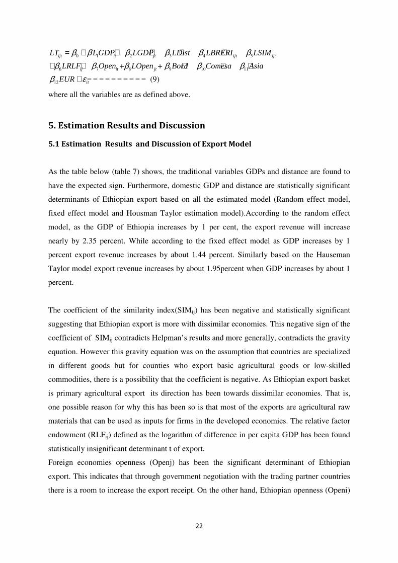
5.1 Estimation Results and Discussion of Export Model

As the table below (table 7) shows, the traditional variables GDPs and distance are found to

have the expected sign. Furthermore, domestic GDP and distance are statistically significant

determinants of Ethiopian export based on all the estimated model (Random effect model,

fixed effect model and Housman Taylor estimation model).According to the random effect

model, as the GDP of Ethiopia increases by 1 per cent, the export revenue will increase

nearly by 2.35 percent. While according to the fixed effect model as GDP increases by 1

percent export revenue increases by about 1.44 percent. Similarly based on the Hauseman

Taylor model export revenue increases by about 1.95percent when GDP increases by about 1

percent.

The coefficient of the similarity index(SIMij) has been negative and statistically significant

suggesting that Ethiopian export is more with dissimilar economies. This negative sign of the

coefficient of SIMij contradicts Helpman’s results and more generally, contradicts the gravity

equation. However this gravity equation was on the assumption that countries are specialized

in different goods but for counties who export basic agricultural goods or low-skilled

commodities, there is a possibility that the coefficient is negative. As Ethiopian export basket

is primary agricultural export its direction has been towards dissimilar economies. That is,

one possible reason for why this has been so is that most of the exports are agricultural raw

materials that can be used as inputs for firms in the developed economies. The relative factor

endowment (RLFij) defined as the logarithm of difference in per capita GDP has been found

statistically insignificant determinant t of export.

Foreign economies openness (Openj) has been the significant determinant of Ethiopian

export. This indicates that through government negotiation with the trading partner countries

there is a room to increase the export receipt. On the other hand, Ethiopian openness (Openi)

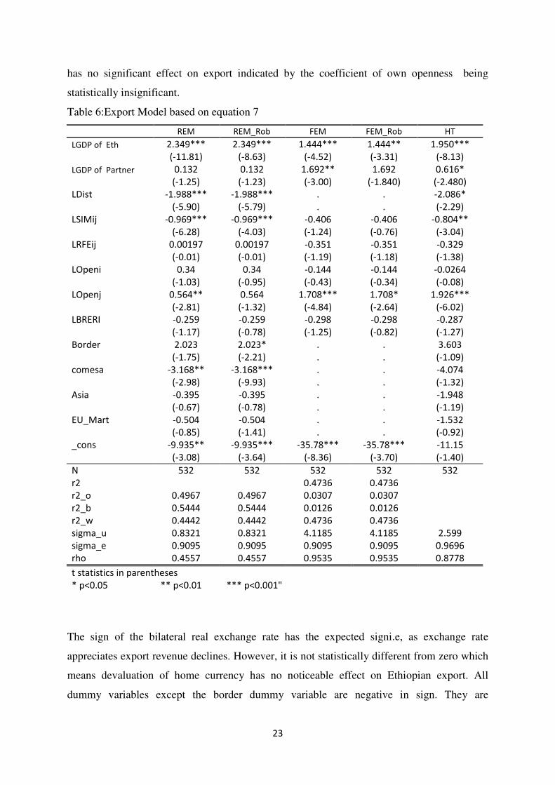
23

has no significant effect on export indicated by the coefficient of own openness being

statistically insignificant.

Table 6:Export Model based on equation 7

REM REM_Rob FEM FEM_Rob HT

LGDP of Eth 2.349*** 2.349*** 1.444*** 1.444** 1.950***

(-11.81) (-8.63) (-4.52) (-3.31) (-8.13)

LGDP of Partner 0.132 0.132 1.692** 1.692 0.616*

(-1.25) (-1.23) (-3.00) (-1.840) (-2.480)

LDist -1.988*** -1.988*** . . -2.086*

(-5.90) (-5.79) . . (-2.29)

LSIMij -0.969*** -0.969*** -0.406 -0.406 -0.804**

(-6.28) (-4.03) (-1.24) (-0.76) (-3.04)

LRFEij 0.00197 0.00197 -0.351 -0.351 -0.329

(-0.01) (-0.01) (-1.19) (-1.18) (-1.38)

LOpeni 0.34 0.34 -0.144 -0.144 -0.0264

(-1.03) (-0.95) (-0.43) (-0.34) (-0.08)

LOpenj 0.564** 0.564 1.708*** 1.708* 1.926***

(-2.81) (-1.32) (-4.84) (-2.64) (-6.02)

LBRERI -0.259 -0.259 -0.298 -0.298 -0.287

(-1.17) (-0.78) (-1.25) (-0.82) (-1.27)

Border 2.023 2.023* . . 3.603

(-1.75) (-2.21) . . (-1.09)

comesa -3.168** -3.168*** . . -4.074

(-2.98) (-9.93) . . (-1.32)

Asia -0.395 -0.395 . . -1.948

(-0.67) (-0.78) . . (-1.19)

EU_Mart -0.504 -0.504 . . -1.532

(-0.85) (-1.41) . . (-0.92)

_cons -9.935** -9.935*** -35.78*** -35.78*** -11.15

(-3.08) (-3.64) (-8.36) (-3.70) (-1.40)

N 532 532 532 532 532

r2

0.4736 0.4736

r2_o 0.4967 0.4967 0.0307 0.0307

r2_b 0.5444 0.5444 0.0126 0.0126

r2_w 0.4442 0.4442 0.4736 0.4736

sigma_u 0.8321 0.8321 4.1185 4.1185 2.599

sigma_e 0.9095 0.9095 0.9095 0.9095 0.9696

rho 0.4557 0.4557 0.9535 0.9535 0.8778

t statistics in parentheses

* p<0.05 ** p<0.01 *** p<0.001"

The sign of the bilateral real exchange rate has the expected signi.e, as exchange rate

appreciates export revenue declines. However, it is not statistically different from zero which

means devaluation of home currency has no noticeable effect on Ethiopian export. All

dummy variables except the border dummy variable are negative in sign. They are

24

statistically insignificant except the Comesa dummy variable, which is statistically significant

unlike the other dummy variables. The negative signs of these variables suggests that

Ethiopia exports below what other countries export to the region. According to the random

effect model, the coefficient of the comesa dummy variable of -3.168 suggests that Ethiopia

exports to the Comesa market 95 percent less or about 4 percent(exp(-3.168 )-1= -0.9579) of

relative to what the rest of the word is trading.

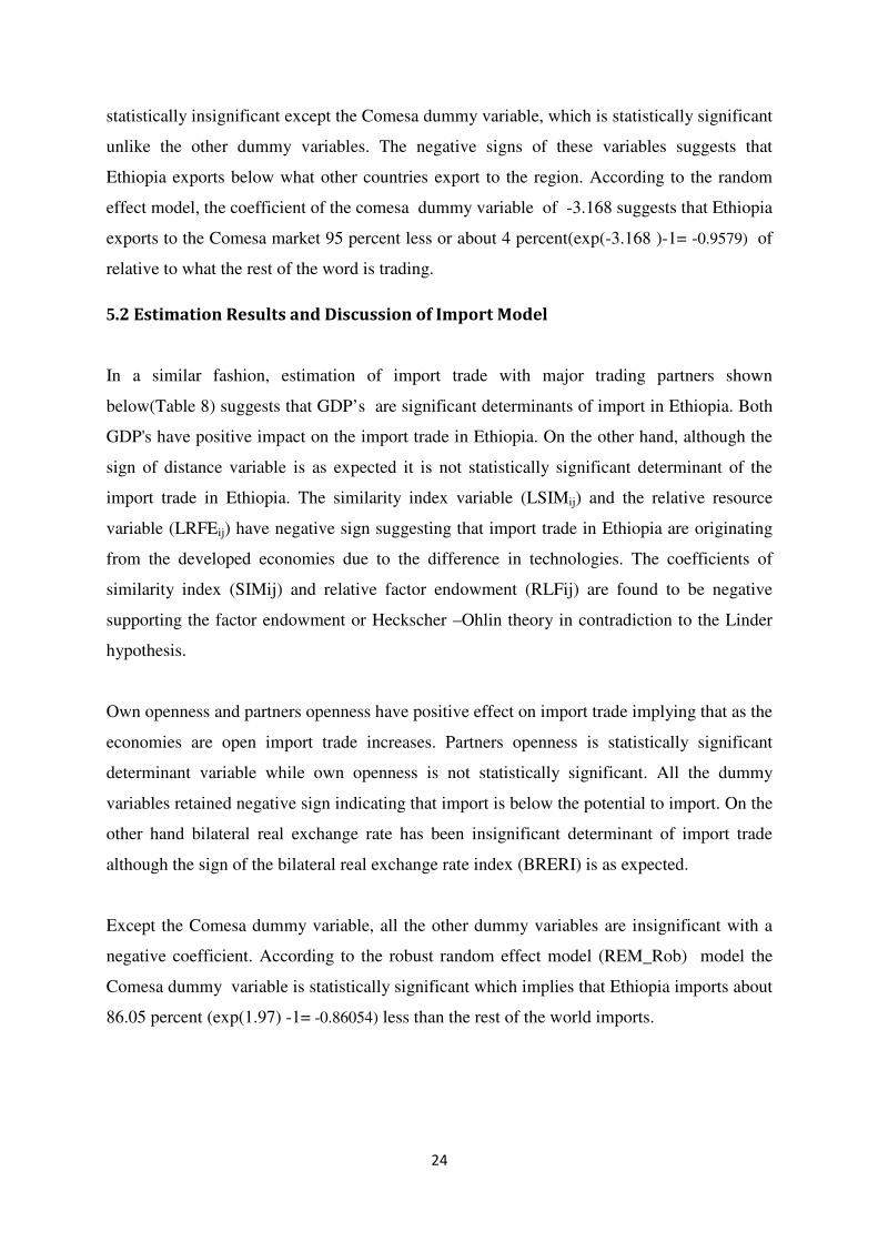
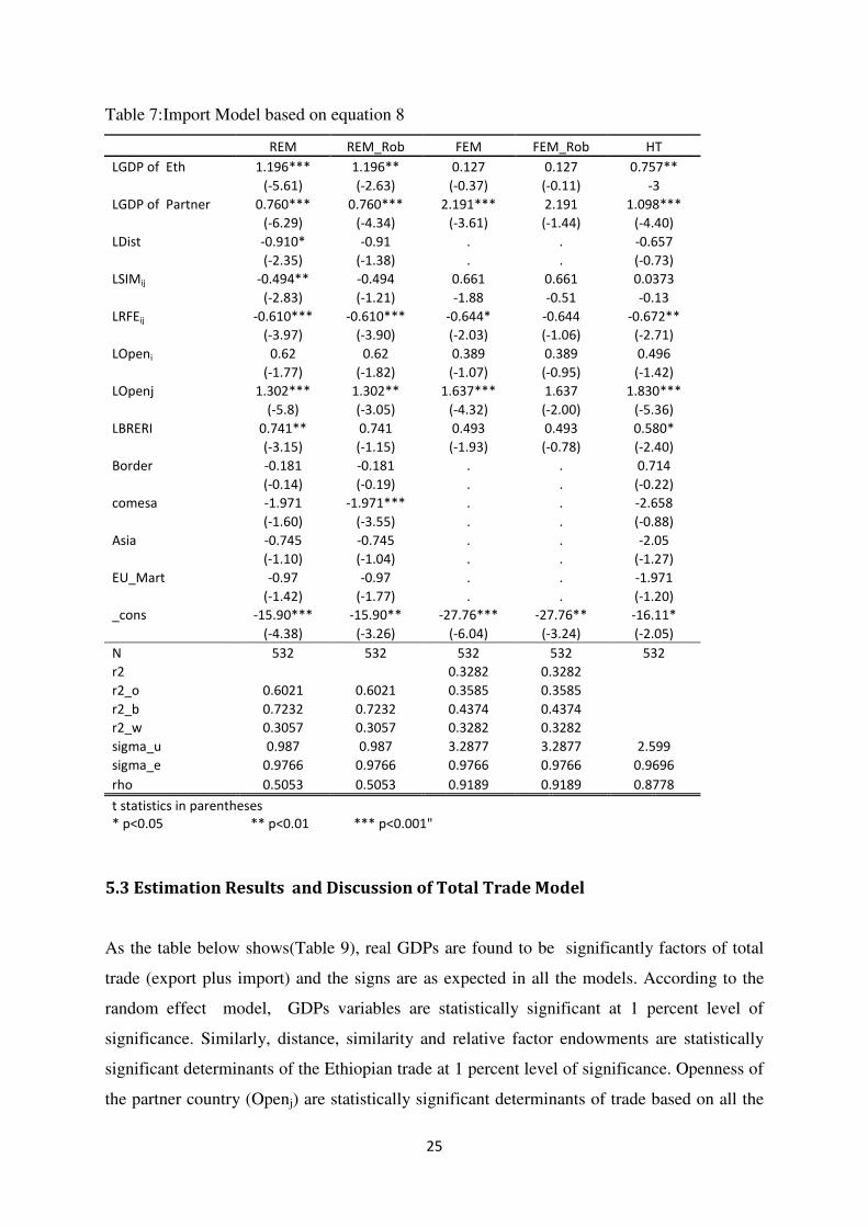
5.2 Estimation Results and Discussion of Import Model

In a similar fashion, estimation of import trade with major trading partners shown

below(Table 8) suggests that GDP’s are significant determinants of import in Ethiopia. Both

GDP's have positive impact on the import trade in Ethiopia. On the other hand, although the

sign of distance variable is as expected it is not statistically significant determinant of the

import trade in Ethiopia. The similarity index variable (LSIMij) and the relative resource

variable (LRFEij) have negative sign suggesting that import trade in Ethiopia are originating

from the developed economies due to the difference in technologies. The coefficients of

similarity index (SIMij) and relative factor endowment (RLFij) are found to be negative

supporting the factor endowment or Heckscher –Ohlin theory in contradiction to the Linder

hypothesis.

Own openness and partners openness have positive effect on import trade implying that as the

economies are open import trade increases. Partners openness is statistically significant

determinant variable while own openness is not statistically significant. All the dummy

variables retained negative sign indicating that import is below the potential to import. On the

other hand bilateral real exchange rate has been insignificant determinant of import trade

although the sign of the bilateral real exchange rate index (BRERI) is as expected.

Except the Comesa dummy variable, all the other dummy variables are insignificant with a

negative coefficient. According to the robust random effect model (REM_Rob) model the

Comesa dummy variable is statistically significant which implies that Ethiopia imports about

86.05 percent (exp(1.97) -1= -0.86054) less than the rest of the world imports.

25

Table 7:Import Model based on equation 8

REM REM_Rob FEM FEM_Rob HT

LGDP of Eth 1.196*** 1.196** 0.127 0.127 0.757**

(-5.61) (-2.63) (-0.37) (-0.11) -3

LGDP of Partner 0.760*** 0.760*** 2.191*** 2.191 1.098***

(-6.29) (-4.34) (-3.61) (-1.44) (-4.40)

LDist -0.910* -0.91 . . -0.657

(-2.35) (-1.38) . . (-0.73)

LSIMij -0.494** -0.494 0.661 0.661 0.0373

(-2.83) (-1.21) -1.88 -0.51 -0.13

LRFEij -0.610*** -0.610*** -0.644* -0.644 -0.672**

(-3.97) (-3.90) (-2.03) (-1.06) (-2.71)

LOpeni 0.62 0.62 0.389 0.389 0.496

(-1.77) (-1.82) (-1.07) (-0.95) (-1.42)

LOpenj 1.302*** 1.302** 1.637*** 1.637 1.830***

(-5.8) (-3.05) (-4.32) (-2.00) (-5.36)

LBRERI 0.741** 0.741 0.493 0.493 0.580*

(-3.15) (-1.15) (-1.93) (-0.78) (-2.40)

Border -0.181 -0.181 . . 0.714

(-0.14) (-0.19) . . (-0.22)

comesa -1.971 -1.971*** . . -2.658

(-1.60) (-3.55) . . (-0.88)

Asia -0.745 -0.745 . . -2.05

(-1.10) (-1.04) . . (-1.27)

EU_Mart -0.97 -0.97 . . -1.971

(-1.42) (-1.77) . . (-1.20)

_cons -15.90*** -15.90** -27.76*** -27.76** -16.11*

(-4.38) (-3.26) (-6.04) (-3.24) (-2.05)

N 532 532 532 532 532

r2 0.3282 0.3282

r2_o 0.6021 0.6021 0.3585 0.3585

r2_b 0.7232 0.7232 0.4374 0.4374

r2_w 0.3057 0.3057 0.3282 0.3282

sigma_u 0.987 0.987 3.2877 3.2877 2.599

sigma_e 0.9766 0.9766 0.9766 0.9766 0.9696

rho 0.5053 0.5053 0.9189 0.9189 0.8778

t statistics in parentheses

* p<0.05 ** p<0.01 *** p<0.001"

5.3 Estimation Results and Discussion of Total Trade Model

As the table below shows(Table 9), real GDPs are found to be significantly factors of total

trade (export plus import) and the signs are as expected in all the models. According to the

random effect model, GDPs variables are statistically significant at 1 percent level of

significance. Similarly, distance, similarity and relative factor endowments are statistically

significant determinants of the Ethiopian trade at 1 percent level of significance. Openness of

the partner country (Openj) are statistically significant determinants of trade based on all the

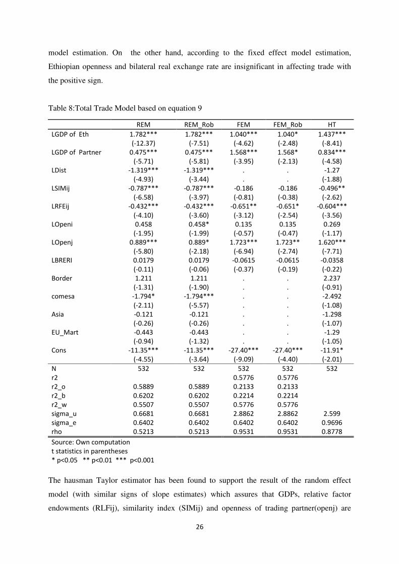
26

model estimation. On the other hand, according to the fixed effect model estimation,

Ethiopian openness and bilateral real exchange rate are insignificant in affecting trade with

the positive sign.

Table 8:Total Trade Model based on equation 9

REM REM_Rob FEM FEM_Rob HT

LGDP of Eth 1.782*** 1.782*** 1.040*** 1.040* 1.437***

(-12.37) (-7.51) (-4.62) (-2.48) (-8.41)

LGDP of Partner 0.475*** 0.475*** 1.568*** 1.568* 0.834***

(-5.71) (-5.81) (-3.95) (-2.13) (-4.58)

LDist -1.319*** -1.319*** . . -1.27

(-4.93) (-3.44) . . (-1.88)

LSIMij -0.787*** -0.787*** -0.186 -0.186 -0.496**

(-6.58) (-3.97) (-0.81) (-0.38) (-2.62)

LRFEij -0.432*** -0.432*** -0.651** -0.651* -0.604***

(-4.10) (-3.60) (-3.12) (-2.54) (-3.56)

LOpeni 0.458 0.458* 0.135 0.135 0.269

(-1.95) (-1.99) (-0.57) (-0.47) (-1.17)

LOpenj 0.889*** 0.889* 1.723*** 1.723** 1.620***

(-5.80) (-2.18) (-6.94) (-2.74) (-7.71)

LBRERI 0.0179 0.0179 -0.0615 -0.0615 -0.0358

(-0.11) (-0.06) (-0.37) (-0.19) (-0.22)

Border 1.211 1.211 . . 2.237

(-1.31) (-1.90) . . (-0.91)

comesa -1.794* -1.794*** . . -2.492

(-2.11) (-5.57) . . (-1.08)

Asia -0.121 -0.121 . . -1.298

(-0.26) (-0.26) . . (-1.07)

EU_Mart -0.443 -0.443 . . -1.29

(-0.94) (-1.32) . . (-1.05)

Cons -11.35*** -11.35*** -27.40*** -27.40*** -11.91*

(-4.55) (-3.64) (-9.09) (-4.40) (-2.01)

N 532 532 532 532 532

r2

0.5776 0.5776

r2_o 0.5889 0.5889 0.2133 0.2133

r2_b 0.6202 0.6202 0.2214 0.2214

r2_w 0.5507 0.5507 0.5776 0.5776

sigma_u 0.6681 0.6681 2.8862 2.8862 2.599

sigma_e 0.6402 0.6402 0.6402 0.6402 0.9696

rho 0.5213 0.5213 0.9531 0.9531 0.8778

Source: Own computation

t statistics in parentheses

* p<0.05 ** p<0.01 *** p<0.001

The hausman Taylor estimator has been found to support the result of the random effect

model (with similar signs of slope estimates) which assures that GDPs, relative factor

endowments (RLFij), similarity index (SIMij) and openness of trading partner(openj) are

27

statistically significant determinants of Ethiopian merchandise trade. Like the earlier

estimators (REM and FEM), the Hausman Taylor (HT) estimator once again confirmed that

own openness and real bilateral exchange rate age insignificant determinants of the Ethiopian

merchandise trade although the coefficients are with expected signs.

As can be seen from the above table, except the comesa dummy variable none of the dummy

variables are significant in affecting the merchandise trade of the country. The dummy

variable Border has positive sign suggesting that there has been more trade with the

neighbouring countries however, the border dummy variable is not statistically signifacant.

While all the other dummy variables are have negative coefficient implying that Ethiopian

merchandise trade with Asia and EU_Market is less than what the rest of the world is trading

with these markets.

5.4 ESTIMATING TRADE POTENTIAL

5.4.1. Estimating Ethiopia’s Export potential

After obtaining the elasticieties of the results of the gravity models for export trade flows, it

is important to estimate export trade potential for Ethiopia. For the estimation of the trade

potential, the estimated coefficients obtained in section 4.1 is used to predict Ethiopia’s

export trade with all the countries in our sample. Among the models estimated in the earlier

section, the random effect model(REM) is used to predict the export trade potential. This is

because of the fact that in the fixed effect model (FEM) some variables will wipe out.

Table 9:Elasticities for the estimation of potential Export

LX Coef. Std. Err. z P>z [95% Conf. Interval]

Lgdpi 2.3488 0.1988 11.8100 0.0000 1.9592 2.7384

Lgdpj 0.1318 0.1056 1.2500 0.2120 -0.0752 0.3387

LDist -1.9883 0.3368 -5.9000 0.0000 -2.6485 -1.3282

LSIMij -0.9686 0.1542 -6.2800 0.0000 -1.2709 -0.6663

LRFEij 0.0020 0.1359 0.0100 0.9880 -0.2645 0.2684

LOpeni 0.3404 0.3307 1.0300 0.3030 -0.3078 0.9886

LOpenj 0.5643 0.2009 2.8100 0.0050 0.1706 0.9581

LBRERI -0.2586 0.2212 -1.1700 0.2420 -0.6921 0.1749

Border 2.0233 1.1542 1.7500 0.0800 -0.2389 4.2854

comesa -3.1679 1.0619 -2.9800 0.0030 -5.2491 -1.0867

Asia -0.3950 0.5886 -0.6700 0.5020 -1.5487 0.7586

EU_Mart -0.5039 0.5897 -0.8500 0.3930 -1.6598 0.6520

cons -9.9354 3.2250 -3.0800 0.0020 -16.2564 -3.6145

Source: own estimates (REM estimation)

The ratio of predicted export trade (P) obtained by the model and actual trade (A) i.e. (P/A) is

then used to analyse the Ethiopia’s global trade potential. Ethiopia (countryi) has trade

28

potential with country j if the value of (Pij/Aij) is greater than one. Under this situation,

attempts for Ethiopia’s trade expansion with country j are recommended.

To see the dynamics on export trade the writer calculated the potential for three different

periods. These are first period since 2008 to see if there are changes on trading pattern after

the global economic recession and since 2000 to examine trade patterns after the Ethio-

Eritrean war. Finally trade potential is calculated for the whole period commencing 1998.

Table 10 below shows that Ethiopia has high export trade potential with countries like

Djibouti, Kenya, Spain, Russia, Portugal, Thailand, Indonesia, France, Hong Hong, Yemen,

India and Singapore, Sweden, Greece, Finland, Japan, South Korea and USA. On the other

hand export to the trading partners such as Switzerland, Somalia, Netherlands, Sudan, China,

Belgium and Pakistan has been already exploited.

Ethiopia’s export trade potentially attain eight times more than currently exported to Djibouti

and Malaysia as to the recent(2008-2011 data) estimation result, seven times more trade with

Kenya, five times more trade with Spain and Russia based on the latest trade profile of after

2008. Results on overall sample period, (1998-2011) confirm that Ethiopia has high export

trade potential with countries such as Kenya, Turkey, Portugal, S.Korea, Russia and Spain.

On the Contrary, Ethiopia's export trade has reached to its maturity level with countries like

Belgium, Switzerland, Pakistan, Israel, Japan, Germany.

29

Table 10:Ethiopian Export Trade Potential

2008-20011 2000-20011 1998-20011

Country Potential Country Potential Country Potential

Djibouti 8.7729 Kenya 14.3599 Kenya 36.3519

Malaysia 8.3856 Spain 5.4095 Turkey 7.4256

Kenya 6.8172 Djibouti 4.4026 Portugal 5.4148

Spain 5.1503 Russia 4.3264 S.Korea 4.7170

Russia 4.6909 S.Korea 4.2126 Spain 4.6914

Portugal 4.4791 Malaysia 3.4675 Russia 3.6867

Thailand 3.5565 Portugal 3.3767 Sudan 3.6757

Indonesia 2.6793 Turkey 2.7959 Djibouti 3.5885

France 2.3472 Finland 2.7452 Thailand 2.9621

Hong Kong 2.3062 Thailand 2.4398 Malaysia 2.8144

Yemen 2.2812 France 1.9529 Hong Kong 2.5268

India 2.0280 Egypt 1.9458 Finland 2.3952

Singapore 1.6239 Indonesia 1.9098 Singapore 2.1501

Canada 1.6108 Hong Kong 1.7335 India 2.1490

Egypt 1.5971 India 1.6396 South Africa 1.7730

Greece 1.5412 Yemen 1.5628 France 1.6960

Sweden 1.5287 South Africa 1.5323 China 1.6463

S.Korea 1.4418 Somalia 1.5323 Indonesia 1.6197

Finland 1.4062 Greece 1.4662 Egypt 1.6186

Japan 1.3881 Sweden 1.3875 Yemen 1.5249

USA 1.2573 Singapore 1.3709 Greece 1.5101

Italy 1.1039 USA 1.3124 Sweden 1.3316

United Kingdom 1.0587 Australia 1.1784 USA 1.2412

Turkey 0.8595 United Kingdom 1.1114 Somalia 1.2137

Saudi Arabia 0.8333 Canada 1.1084 Australia 1.1224

U.Arab Emirates 0.7516 Sudan 1.0482 United Kingdom 1.0982

South Africa 0.6508 U.Arab Emirates 0.9398 U. Arab Emirates 1.0846

Germany 0.5954 Italy 0.8362 Canada 0.9413

Australia 0.5953 Saudi Arabia 0.8080 Italy 0.7644

Israel 0.4944 Netherlands 0.7187 Saudi Arabia 0.7184

Jordan 0.4925 Jordan 0.6540 Netherlands 0.6853

Pakistan 0.3777 Germany 0.6263 Jordan 0.6462

Belgium 0.3159 Japan 0.6212 Germany 0.5358

China 0.3099 China 0.5071 Japan 0.5080

Sudan 0.2502 Israel 0.4804 Israel 0.4625

Netherlands 0.2204 Pakistan 0.4240 Pakistan 0.3813

Switzerland 0.1321 Belgium 0.3358 Switzerland 0.3446

Somalia 0.0575 Switzerland 0.1461 Belgium 0.3048

Source: Model estimation

5.5.2. Estimating Ethiopia’s Import Trade Potential

Like the case in the export trade potential estimation ,after obtaining the elasticities of the

results of the gravity models for import trade, they are used to estimate import trade potential

30

for Ethiopia. In doing so, the elasticities used to estimate the potential are those obtained

from the random effect model for the fact that time invariance variables will be dropped in

using the fixed effect model. So the following table shows the elasticieties to be used in

estimating the import trade potential.

Table 11:Elasticities for the estimation of potential Import

LM Coef. Std. Err. z P>z [95% Conf. Interval]

Lgdpi 1.1961 0.2134 5.6100 0.0000 0.7779 1.6143

Lgdpj 0.7602 0.1208 6.2900 0.0000 0.5235 0.9968

LDist -0.9105 0.3878 -2.3500 0.0190 -1.6705 -0.1505

LSIMij -0.4944 0.1744 -2.8300 0.0050 -0.8363 -0.1525

LRFEij -0.6100 0.1536 -3.9700 0.0000 -0.9111 -0.3088

LOpeni 0.6198 0.3501 1.7700 0.0770 -0.0664 1.3060

LOpenj 1.3019 0.2244 5.8000 0.0000 0.8621 1.7417

LBRERI 0.7412 0.2353 3.1500 0.0020 0.2801 1.2024

Border -0.1809 1.3344 -0.1400 0.8920 -2.7964 2.4346

comesa -1.9711 1.2294 -1.6000 0.1090 -4.3807 0.4385

Asia -0.7448 0.6790 -1.1000 0.2730 -2.0756 0.5861

EU_Mart -0.9697 0.6817 -1.4200 0.1550 -2.3058 0.3663

cons -15.9025 3.6337 -4.3800 0.0000 -23.0244 -8.7806

Source: Model estimation

once estimating the elasticities through the random effect model, they are going to be used in

the process of estimating the potential import of merchandise trade in Ethiopia. The first task

was to predict the import values from the model and comparing the predicted value and

the actual import trade values as the case in the export trade calculations above. That is, the

ratio of predicted import trade (P) obtained by the model and actual trade (A) can be used to

estimate the potential i.e. (P/A). Ethiopia (countryi) has trade potential with country j if the

value of (Pij/Aij) is greater than one.

According to the recent merchandise trade statistics(2008-2011) there is a great potential of

import from countries such as Hong Kong, Singapore, Egypt, Somalia, Portugal, Yemen,

Australia, United Kingdom, Germany, Finland, Israel and USA. On the other hand, import

trade from countries such as Canada, Soudi Arabia, United Arab Emirates, Japan, Turkey,

Malaysia, Italy, Pakistan, Sweden and China has already reached to its maturity stage that it

cannot be increased much more. In the same way, the overall import trade potential of the

country is on these countries that trade negotiation and marketing strategies to penetrate the

markets in these countries should be promoted so as to reap the benefits of trade. This could

help the domestic economy to import technology and diversify its import markets so that the

problem of dependence on few markets.

31

Table 12:Ethiopian Import Trade Potential

2008-20011 2000-20011 1998-20011

Country Potential Country Potential Country Potential

Hong Kong 8.0536 Hong Kong 26.7479 Hong Kong 29.1603

Singapore 7.3978 Somalia 9.5490 Sudan 25.4135

Egypt 3.5632 Portugal 5.8802 Portugal 8.3373

Somalia 2.7643 Singapore 5.2177 Somalia 7.8351

Greece 2.5415 Egypt 2.8349 Pakistan 4.9950

Portugal 2.3925 Pakistan 2.7785 Singapore 4.5012

Yemen 2.3312 Yemen 2.4509 Russia 3.0198

Australia 2.1311 Spain 2.2844 Egypt 2.8623

United Kingdom 2.0180 Russia 2.2126 Spain 2.2267

Germany 1.9050 Australia 1.8441 Yemen 2.1005

Finland 1.7211 Greece 1.7889 Australia 1.7622

Israel 1.5703 Germany 1.6213 USA 1.6421

USA 1.5621 USA 1.4421 Thailand 1.5653

Spain 1.4578 Thailand 1.3883 Greece 1.5602

Netherlands 1.3231 United Kingdom 1.3198 Germany 1.4980

India 1.3180 Israel 1.2976 India 1.2193

Jordan 1.2563 India 1.2186 Israel 1.2021

France 1.1943 Netherlands 1.1366 Netherlands 1.1899

Russia 1.1462 France 1.1184 United Kingdom 1.1688

Thailand 0.9894 Jordan 1.0853 South Africa 1.0908

Switzerland 0.8515 Finland 0.9604 Finland 1.0841

S.Korea 0.8438 Malaysia 0.8895 France 1.0757

Belgium 0.8070 South Africa 0.8862 Malaysia 1.0636

South Africa 0.7341 Belgium 0.8465 Jordan 1.0339

Indonesia 0.6963 Switzerland 0.8186 China 0.9064

Kenya 0.6064 China 0.7420 Belgium 0.8754

China 0.5026 S.Korea 0.6560 Switzerland 0.7659

Sweden 0.4511 Indonesia 0.6354 Indonesia 0.6999

Pakistan 0.3996 Sudan 0.6036 S.Korea 0.5778

Italy 0.3425 Kenya 0.4143 Turkey 0.4431

Malaysia 0.3387 Turkey 0.3804 Kenya 0.3685

Turkey 0.2731 U. Arab Emirates 0.3551 Saudi Arabia 0.3490

Japan 0.2681 Sweden 0.3543 Italy 0.3484

U. Arab Emirates 0.2153 Italy 0.3374 U.Arab Emirates 0.3311

Saudi Arabia 0.1992 Japan 0.2367 Sweden 0.3308

Canada 0.1625 Saudi Arabia 0.2250 Japan 0.2331

Sudan 0.0991 Canada 0.1591 Canada 0.1648

Source: Model estimation

5.5.3. Estimating Ethiopia’s Total Trade Potential

Similarly as in the case of export and import trade potential estimations, after obtaining the

elasticieties from the estimated results of the gravity models for bilateral total trade flows the

estimation process proceeded to quantify total trade potential for Ethiopia. In this section the

32

writer has used the estimated coefficients obtained in section 4.3 to predict Ethiopia’s total

trade with all the countries in our sample. The ratio of predicted total trade (P) obtained by

the model and actual trade (A) i.e. (P/A) is then used to analyse the Ethiopia’s global total

trade potential. Ethiopia (country i) has trade potential with country j if the value of (Pij/Aij)

is greater than one.

Table 13:Elasticities for the estimation of potential Import

LTij Coef. Std. Err. z P>z [95% Conf. Interval]

Lgdpi 1.7819 0.1441 12.3700 0.0000 1.4995 2.0642

Lgdpj 0.4747 0.0832 5.7100 0.0000 0.3116 0.6377

LDist -1.3192 0.2677 -4.9300 0.0000 -1.8440 -0.7945

LSIMij -0.7872 0.1197 -6.5800 0.0000 -1.0218 -0.5526

LRFEij -0.4317 0.1054 -4.1000 0.0000 -0.6382 -0.2251

LOpeni 0.4579 0.2352 1.9500 0.0520 -0.0031 0.9190

LOpenj 0.8892 0.1533 5.8000 0.0000 0.5888 1.1897

LBRERI 0.0179 0.1583 0.1100 0.9100 -0.2924 0.3283

Border 1.2111 0.9227 1.3100 0.1890 -0.5974 3.0196

comesa -1.7944 0.8505 -2.1100 0.0350 -3.4613 -0.1274

Asia -0.1209 0.4691 -0.2600 0.7970 -1.0404 0.7986

EU_Mart -0.4427 0.4713 -0.9400 0.3480 -1.3664 0.4811

Cons -11.3503 2.4933 -4.5500 0.0000 -16.2371 -6.4635

Source: Model Estimation

Like the case for export and import trade to see the dynamics on trade the potential for three

different periods were calculated. These are for the first period 2008-2011 to see if there are

changes on trading pattern after the global economic recession and 2000-2011 to examine

trade patterns after the Ethio-Eritrean war. Finally trade potential is calculated for the whole

period since 1998.

Results for the three periods suggested that Ethiopia has the highest total trade potential with

countries like Hong Kong, Djibouti, Singapore, Yemen Kenya, Spain, Russia, Portugal,

United Kingdom, Egypt, France Finland, Germany, India . Ethiopia’s total trade potential

attain eight times more than what actually traded with Djibouti, six times more with Hong

Kong four times more trade with Singapore and Yemen and more than twice with Spain

,Portugal, Greece and Kenya as of 2008.

Results on overall sample period, (since 1998) confirm that Ethiopia has the highest total

trade potential with the above countries particularly Hong Kong, Sudan, Portugal, Djibouti,

Spain, Yemen, Russia, Somalia, Singapore, and Pakistan.

33

Table 14:Total Merchandise Trade Potential

2008-20011 2000-20011 1998-20011

Country

Potential Country Potential Country

Potential

Djibouti 8.2229 Hong Kong 8.8731 Hong Kong 10.334

Hong Kong 6.4139 Djibouti 4.3228 Sudan 7.1829

Singapore 3.9759 Spain 3.2156 Portugal 5.2874

Yemen 3.8242 Somalia 3.1791 Djibouti 3.5768

Kenya 3.6395 Yemen 3.0050 Spain 2.9936

Portugal 2.7807 Singapore 2.8457 Yemen 2.5704

Greece 2.4208 Portugal 2.3786 Russia 2.5418

Spain 2.2080 Kenya 2.2880 Somalia 2.5215

United Kingdom 1.8988 Russia 2.2858 Singapore 2.4689

Egypt 1.8719 Sudan 2.0682 Pakistan 2.2203

France 1.7675 Greece 1.9199 Kenya 1.9863

Finland 1.5885 Pakistan 1.8510 Greece 1.7081

Russia 1.5417 France 1.6274 France 1.5157

Germany 1.4923 Egypt 1.5583 Egypt 1.5069

India 1.3955 Germany 1.4393 USA 1.4036

USA 1.3118 United Kingdom 1.4361 Thailand 1.3761

Indonesia 1.1499 India 1.3136 India 1.3267

Thailand 1.0497 USA 1.2737 United Kingdom 1.306

S.Korea 1.0277 Thailand 1.2235 Germany 1.2858

Australia 1.0231 Australia 1.1622 Australia 1.1165

Israel 0.8649 Finland 1.0142 South Africa 1.0964

Canada 0.7927 Indonesia 0.9294 Finland 1.0571

Jordan 0.7904 S.Korea 0.8990 Indonesia 0.9139

Sweden 0.7723 South Africa 0.8901 Netherlands 0.8727

South Africa 0.6856 Jordan 0.8397 Jordan 0.8523

Netherlands 0.6618 Netherlands 0.8257 China 0.8247

Belgium 0.5900 Israel 0.7388 S.Korea 0.7987

Italy 0.5707 China 0.6680 Malaysia 0.7478

Sudan 0.5043 Malaysia 0.6633 Israel 0.7181

Turkey 0.4813 Belgium 0.6338 Turkey 0.704

China 0.4803 Canada 0.6285 Belgium 0.617

Japan 0.4285 Turkey 0.6167 Canada 0.5804

Pakistan 0.4256 Italy 0.5441 Italy 0.5424

Switzerland 0.3424 Sweden 0.5266 Sweden 0.4761

Saudi Arabia 0.3063 U. Arab Emirates 0.4702 U.Arab Emirates 0.4665

Malaysia 0.3051 Switzerland 0.3800 Saudi Arabia 0.4389

U. Arab Emirates 0.2738 Japan 0.3595 Switzerland 0.3987

Somalia 0.1106 Saudi Arabia 0.3576 Japan 0.3468

Source: Model Estimation

34

6. Conclusions and Recommendations

6.1 Conclusions

The performance of the foreign trade in Ethiopia has shown a tremendous progress. over the

last ten years. The export receipt of the country is so small that it cannot finance import

payments of the country. For this reason, trade deficit is widening very much as the export

basket and destinations are limited and the import demand is growing following the growing

income of consumers. It is therefore important to identify the factors that can help to develop

the export receipt. In doing so, the gravity model of trade was developed for export, import

and total trade of the country.

The study shows that traditional variables of the gravity model(GDP's) are significant

determinants of the trade in the country. Similarly, the distance variable which is the proxied

variable for transport and logistics related factors is also significant determinant of the trade.

Openness of trading partner country is found to be significant determinant of trade while

exchange rate is not found to be affecting trade although the sign is as expected. The

similarity index is also found to be significant factors of trade with negative sign suggesting

trade in Ethiopia is with dissimilar economies which is in contradiction of Helpman's

theorem. This shows that Ethiopia's trade is due to difference in technology and the trade in

not intera industry trade that existed in Ethiopia. The relative factor endowment

variable(LRFEij) which stands for change in resource endowments or relative difference in

wealth is affecting the volume of trade in Ethiopia. Accordingly, as the difference in wealth

increased the trade flow continued to grow. The dummy variable for the Comesa maket is

statistically significant and negative in sign indicating that trade in the Comesa market is less

than which it should have to be. According to the estimated gravity models, Ethiopia trade to

the Comesa member countries less than 5 percent of its potential.

From the gravity model using the estimated elasticieties, trade values for countries are

predicted. Using the predicted values, attempts have been made to estimate trade potential for

countries. According to the estimated results, Ethiopia has unexploited export potential with

Djibouti and Malaysia, Kenya, Spain and Russia. Results on overall sample period, (1998-

2011) confirm that Ethiopia has high export trade potential with countries such as Kenya,

35

Turkey, Portugal, S.Korea, Russia and Spain. On the Contrary, Ethiopia's export trade has

reached to its maturity level with countries like Belgium, Switzerland, Pakistan, Israel, Japan,

Germany. Similarly, there is a great potential of import from countries such as Hong Kong,

Singapore, Egypt, Somalia, Portugal, Yemen, Australia, United Kingdom, Germany, Finland,

Israel and USA. On the other hand, import trade from countries such as Canada, Saudi

Arabia, United Arab Emirates, Japan, Turkey, Malaysia, Italy, Pakistan, Sweden and China

has already reached to its maturity.

6.2 Recommendations

Trade deficit has continued to be one of the sources of macroeconomic instability in

Ethiopia. Openness of the partner economies are one of the determinants of the export as well

as import trade in Ethiopia. Ethiopia's trade is directed/originated to few destination

countries. It is important to expand export destinations. One possible destinations could be

the Comesa member countries .There are countries in which trade(export and import)

potentials are unexploited. Therefore, it is crucial to do the following policy options to

expand export receipt and narrow trade deficit.

1. Government needs to aggressively engage a bilateral trade negotiations with countries

that Ethiopia has a potential.

2. Government should encourage the private sectors to develop market innovations with

which Ethiopia has export potential through various incentive packages.

3. By identifying countries with which Ethiopia has export potential, government should

help the private sector in market innovation by opening business missionaries that

conduct and provide up-to-date information to the exporters and make promotional

works to the export trade sector .

4. The trade record in Ethiopia shows that most export destinations are European

markets and imports origin from Asia particularly China and Saudi Arabia as well as

United Arab Emirates .The country needs to maximize its share from the American

market (AGO opportunities) through creating value addition and by working on

quality of products to exported.

36