Detecting Small Moving Targets in Infrared Imagery
64
University of Central Florida University of Central Florida STARS STARS Electronic Theses and Dissertations, 2020- 2020 Detecting Small Moving Targets in Infrared Imagery Detecting Small Moving Targets in Infrared Imagery Adam Cuellar University of Central Florida Part of the Computer Engineering Commons Find similar works at: https://stars.library.ucf.edu/etd2020 University of Central Florida Libraries http://library.ucf.edu This Masters Thesis (Open Access) is brought to you for free and open access by STARS. It has been accepted for inclusion in Electronic Theses and Dissertations, 2020- by an authorized administrator of STARS. For more information, please contact [email protected]. STARS Citation STARS Citation Cuellar, Adam, "Detecting Small Moving Targets in Infrared Imagery" (2020). Electronic Theses and Dissertations, 2020-. 344. https://stars.library.ucf.edu/etd2020/344
Transcript of Detecting Small Moving Targets in Infrared Imagery

University of Central Florida University of Central Florida
STARS STARS
Electronic Theses and Dissertations, 2020-
2020
Detecting Small Moving Targets in Infrared Imagery Detecting Small Moving Targets in Infrared Imagery
Adam Cuellar University of Central Florida
Part of the Computer Engineering Commons
Find similar works at: https://stars.library.ucf.edu/etd2020
University of Central Florida Libraries http://library.ucf.edu
This Masters Thesis (Open Access) is brought to you for free and open access by STARS. It has been accepted for
inclusion in Electronic Theses and Dissertations, 2020- by an authorized administrator of STARS. For more
information, please contact [email protected].
STARS Citation STARS Citation Cuellar, Adam, "Detecting Small Moving Targets in Infrared Imagery" (2020). Electronic Theses and Dissertations, 2020-. 344. https://stars.library.ucf.edu/etd2020/344

DETECTING SMALL MOVING TARGETS IN INFRARED IMAGERY
by
ADAM THOMAS CUELLAR B.S. University of Central Florida, 2019
A thesis submitted in partial fulfillment of the requirements for the degree of Master of Science
in the Department of Electrical and Computer Engineering in the College of Engineering & Computer Science
at the University of Central Florida Orlando, Florida
Fall Term 2020
Major Professor: Abhijit Mahalanobis

ii
ABSTRACT
Deep convolutional neural networks have achieved remarkable results for
detecting large and medium sized objects in images. However, the ability to detect small
objects has yet to achieve the same level performance. Our focus is on applications that
require the accurate detection and localization of small moving objects that are distant
from the sensor. We first examine the ability of several state-of-the-art object detection
networks (YOLOv3 and Mask R-CNN [1] [2]) to find small moving targets in infrared
imagery using a publicly released dataset by the US Army Night Vision and Electronic
Sensors Directorate. We then introduce a novel Moving Target Indicator Network
(MTINet) and repurpose a hyperspectral imagery anomaly detection algorithm, the Reed-
Xiaoli detector [3], for detecting small moving targets. We analyze the robustness and
applicability of these methods by introducing simulated sensor movement to the data.
Compared with other state-of-the-art methods, MTINet and the ARX algorithm achieve a
higher probability of detection at lower false alarm rates. Specifically, the combination of
the algorithms results in a probability of detection of approximately 70% at a low false
alarm rate of 0.1, which is about 50% greater than that of YOLOv3 and 65% greater than
Mask R-CNN.

iii
ACKNOWLEDGEMENTS
I would like to extend my sincere and heartfelt gratitude to my advisor Professor
Abhijit Mahalanobis for the continuous support of my Masters research and his immense
knowledge and experience in computer vision. His guidance has helped me gain a true
understanding of computer vision applied to real world scenarios.
I would also like to thank my fellow colleagues at Lockheed Martin, William
McDowell and Nicholas Shorter, for directing my knowledge of deep learning and its
application in computer vision. Both have encouraged me to continue learning and have
offered me opportunities to practice my knowledge on novel datasets.
iv
TABLE OF CONTENTS
LIST OF FIGURES ..........................................................................................................vi
LIST OF TABLES ........................................................................................................... vii
LIST OF ACRONYMS ................................................................................................... viii
CHAPTER ONE: INTRODUCTION ................................................................................. 1
NVESD Dataset ........................................................................................................... 2
Literature Review ......................................................................................................... 4
YOLOv3 ................................................................................................................... 4
Mask R-CNN ............................................................................................................ 6
ResNeSt ................................................................................................................... 8
Reed-Xiaoli Detector ................................................................................................ 9
Convolutional Neural Network Improvements ........................................................ 10
CHAPTER TWO: PRELIMINARY EXPERIMENTS ....................................................... 14
Dataset Partitioning ................................................................................................... 14
Frame-by-Frame .................................................................................................... 15
Difference Images .................................................................................................. 16
Grouped Frames .................................................................................................... 17
YOLOv3 Results ........................................................................................................ 18
Frame-by-Frame .................................................................................................... 18
Difference Images .................................................................................................. 19
YOLOv3-LSTM Results ............................................................................................. 21
Mask R-CNN Results ................................................................................................. 22
Frame-by-Frame .................................................................................................... 22
Difference Images .................................................................................................. 23
Experiment Analysis .................................................................................................. 24
CHAPTER THREE: METHODOLOGY .......................................................................... 28
MTINet ....................................................................................................................... 28
MTINet-DW ................................................................................................................ 35
Combining MTINet and the Reed-Xiaoli Algorithm .................................................... 37

v
Modeling Sensor Movement ...................................................................................... 38
CHAPTER FOUR: RESULTS ....................................................................................... 40
Evaluation of MTINet-1 using MSE and TCR loss functions ...................................... 40
Evaluation of MTINet-2 and MTINet-CC .................................................................... 42
Evaluation of MTINet-CC with Simulated Sensor Movement ..................................... 44
Performance Evaluation of MTINet-DW ..................................................................... 46
Evaluation of the ARX Algorithm................................................................................ 48
Combining MTINet and the ARX Algorithm ............................................................... 49
CHAPTER FIVE: CONCLUSION AND FUTURE WORK .............................................. 51
REFERENCES .............................................................................................................. 54

vi
LIST OF FIGURES
Figure 1: Example NVESD frames at day and night with targets at different ranges ...... 3
Figure 2: Spatial Pyramid Pooling block .......................................................................... 6
Figure 3: Convolutional Block Attention Module ............................................................ 11
Figure 4: Histogram of Pixels on Target in training and testing set ............................... 15
Figure 5: Example of bi-directional image differencing .................................................. 16
Figure 6: Example of five frame blocks and the registration of two frames ................... 17
Figure 7: YOLOv3 frame-by-frame training and testing set results ............................... 19
Figure 8: YOLOv3 difference images training and testing set results ............................ 20
Figure 9: YOLOv3-LSTM frame-by-frame training and testing set results ..................... 21
Figure 10: Mask R-CNN frame-by-frame training and testing set results ...................... 23
Figure 11: Mask R-CNN difference images training and testing set results .................. 24
Figure 12: Activation Maps of trained feature extractors Darknet53 and ResNeSt50 ... 26
Figure 13: Predictions made by YOLOv3 and Mask R-CNN on successive frames ...... 27
Figure 14: Example of ideal mask ................................................................................. 29
Figure 15: Diagram of MTINet-1 .................................................................................... 32
Figure 16: Diagram of MTINet-2 .................................................................................... 33
Figure 17: Implementation of modified SPP module in MTINet-CC .............................. 35
Figure 18: Modified Convolutional Block Attention Module with a pointwise convolution
...................................................................................................................................... 37
Figure 19: Example of simulated sensor movement ..................................................... 39
Figure 20: MTINet 1 results on NVESD testing set with MSE loss ................................ 41
Figure 21: MTINet 1 results on NVESD testing set with the modified TCR loss ............ 42
Figure 22: MTINet 2 results on NVESD testing set ....................................................... 42
Figure 23: MTINet-CC results on NVESD testing set .................................................... 43
Figure 24: MTINet-CC results on NVESD testing set with misaligned frames ............... 44
Figure 25: MTINet-CC results on NVESD testing set with registered frames ................ 45
Figure 26: MTINet-CC results on NVESD testing set with and without sensor movement
...................................................................................................................................... 46
Figure 27: MTINet-DW results on NVESD testing data with registered frames ............. 47
Figure 28: Activation Map of trained MTINet-DW .......................................................... 48
Figure 29: ARX Algorithm results on NVESD testing data with registered frames ........ 49
Figure 30: Combined MTINet-DW and ARX algorithm results on the NVESD testing data
with registered frames ................................................................................................... 50
Figure 31: Comparison of MTINet-DW, the ARX algorithm, and their combination on the
NVESD testing set......................................................................................................... 50
Figure 32: Comparison of results given simulated sensor movement ........................... 53

vii
LIST OF TABLES
Table 1: Comparison of object detection networks on the MS COCO dataset [1] [2] [7] [8]
for small, medium, and large objects ............................................................................... 2
Table 2: Preliminary experiment results at IOU of 0.5 and score threshold of 0.5 ......... 25
Table 3: Comparing results of highest performance experiments ................................. 52

viii
LIST OF ACRONYMS
AP Average Precision CBAM Convolutional Block Attention Module CNN Convolutional Neural Network FAR False Alarm Rates FOV Field of View IOU Intersection over Union LSTM Long Short-Term Memory mAP Mean Average Precision MS COCO Microsoft Common Objects in Context MSE Mean Squared Error MTINet Moving Target Indicator Network MWIR Mid-Wave Infrared NVESD Night Vision and Electronic Sensors Directorate PCA Principal Component Analysis PDet Probability of Detection POT Pixels on Target R-CNN Region-based Convolutional Neural Network ROC Receiver Operating Characteristic RoI Region of Interest RPN Region Proposal Network SE Squeeze-And-Excitation SOTA State-of-the-art SPP Spatial Pyramid Pooling SURF Speeded Up Robust Features TCR Target to Clutter Ratio YOLO You Only Look Once

1
CHAPTER ONE: INTRODUCTION
High performance, deep convolutional neural network (CNN) based object
detectors have been largely developed for use with RGB data. There are many popular
methods for detecting and localizing objects from images; however, the detection
performance for small objects remains a challenging problem.
Modern CNN’s are benchmarked on common datasets such as ImageNet [4] and
Microsoft common objects in context (MS COCO) [5]. Each of these datasets contains
natural images with discernible features and relatively large objects. MS COCO defines
small, medium, and large objects as those with areas (defined in terms of total pixels) of
area < 322, 322 < area < 962, and area > 962 respectively. Current state-of-the-art (SOTA)
networks, such as You Only Look Once (YOLO) and Mask R-CNN, perform inadequately
on the small objects in the COCO dataset. [6]
As shown in Table 1, the performance of detectors on medium and large objects
significantly surpasses their performance on small objects. The average precision (AP)
on large objects is more than twice of that on small objects for each of these networks.
Therefore, we ask the question: What improvements can be made to increase the
performance of small object detection techniques, and can it be realized on types of
imagery other than RGB data?

2
Table 1: Comparison of object detection networks on the MS COCO dataset [1] [2] [7] [8] for small, medium, and large objects
Network AP APS APM APL
YOLOv3 33.0% 18.3% 35.4% 41.9%
Mask R-CNN 37.1% 16.9% 39.9% 53.5%
First, we aim to tackle this problem by repurposing existing object detection
algorithms for find small moving targets, and systematically evaluating their performance
on infra-red imagery. Specifically, we train and evaluate these algorithms using a publicly
released dataset by the US Army Night Vision and Electronic Sensors Directorate
(NVESD). Both YOLOv3 and Mask R-CNN perform poorly on this dataset with less than
a 20% mean average precision (mAP). This provides the motivation for developing novel
custom CNN networks, and for re-examining other statistical methods such as the Reed-
Xiaoli detector (which is widely used for hyperspectral anomaly detection) for detecting
small moving targets in infra-red imagery.
NVESD Dataset
The data set provided for this research is a collection of mid-wave infrared (MWIR)
imagery collected by the US Army Night Vision and Electronic Sensors Directorate [6].
The data includes vehicular targets moving at a constant velocity along a circle with a
diameter of about 100 meters. This movement allows us to obtain all azimuth angles of
the vehicles. The data was collected at day and night, at different ranges, and contains

3
ten different types of vehicles. These vehicles belong to both military and civilian classes
including BTR70, BMP, BRDM, T62, T72, ZSU23, 2S3, MTLB, SUV, and Pickup truck.
Ground truth information was provided which contained information about the target’s
location, range, and class. The vehicles can be anywhere between 1000 to 5000 meters
in range. Other information is also provided; however, we do not directly use this data.
Figure 1 below shows the diversity between the day and night infrared photos as well as
the relative size of the target within the image.
Figure 1: Example NVESD frames at day and night with targets at different ranges

4
Literature Review
Modern object detection models are generally built in two different ways, two-stage
object detectors and one-stage object detectors. Both types of detectors have a backbone
that is used to extract features and encode data for the head of the network. For a two-
stage network, the head predicts the coordinates of an object and then classifies that
object. For a one-stage network, the head predicts both the coordinates and the
classification of an object simultaneously. One-stage networks are often much faster but
often less accurate [1]. Therefore, we assess the use of each as a benchmark for the
performance of target detection in the NVESD dataset.
YOLOv3
You Only Look Once is a one stage object detection network developed by Joseph
Redmon and Ali Farhadi. The performance of YOLO has improved across different
versions such as YOLO, YOLOv2, YOLOv3 tiny, and YOLOv3. As most object detection
networks, YOLOv3 consists of a feature extractor as well as three separate detection
heads. The feature extractor, Darknet53, is made up of 53 convolutional layers and
outperforms larger models such as Resnet-101 on the ImageNet dataset for classification
[1]. Prediction is done at three different scales using each of the detection heads. Each
head is responsible for reducing the image into a grid of different sizes. Specifically, the
three heads reduce the image into (ℎ
25,𝑤
25), (
ℎ
24,𝑤
24), and (
ℎ
23,𝑤
23) where ℎ and 𝑤 are

5
the height and width of the input image. Each cell in the grid is responsible for predicting
an object if the object’s center falls within that cell. The output of each head is a 3D tensor
encoding bounding box coordinates, the objectness of the detections, and class
predictions. The bounding box coordinates output by the detection head are an offset
from the top left corner of the image added to a proportion of the bounding box priors.
The bounding box priors, or anchors, are computed using k-means clustering on all
bounding boxes found in the training set.
The original loss functions for YOLOv3 is composed of the mean squared error
(MSE) of the bounding box coordinates, the binary cross entropy of the objectness score,
and the binary cross entropy of the multi-class predictions of each bounding box. This
loss function since has been improved by removing the MSE of the bounding box
coordinates and substituting the intersection over union (IOU) loss. The intersection over
union is the area of intersection between the predicted bounding box and its respective
ground truth divided by the area of union.
Zhanchao Huang and Jianlin Wang first introduced the Spatial Pyramid Pooling
(SPP) block to YOLO using YOLOv2 [9]. The addition of this block increased the mean
average precision of YOLOv2 on the PASCAL VOC2007 test dataset by approximately
2%; therefore, the idea was applied to YOLOv3 as well [9]. The SPP block consists of
three max-pooling layers, each with different kernel sizes. Initially the block contained the
kernel sizes 5x5, 7x7, and 13x13; however, when adding the block to YOLOv3 the 7x7
kernel was replaced with a 9x9 kernel. The addition of this module emphasizes high

6
frequency features within the image thus increasing the networks ability to detect and
classify an object. Figure 2 shows the implementation of the SPP module.
Figure 2: Spatial Pyramid Pooling block
Mask R-CNN
Mask Region-based CNN (R-CNN) is a two-stage detector developed by He et al.
Mask R-CNN is an extension of Faster R-CNN which adds a branch for predicting an
object mask in parallel with the existing bounding box prediction branch. Similar to Faster
R-CNN, the network consists of a region proposal network (RPN) and a classification
stage. The addition of the object mask prediction occurs in the classification stage where
the network is responsible for predicting the class and box offsets. This branch allows for
the output of a binary mask for each region of interest (RoI).

7
In addition to the new branch, Mask R-CNN appends the mask loss 𝐿𝑚𝑎𝑠𝑘 to
Faster R-CNN’s loss function. This multi-task loss function is defined as 𝐿 = 𝐿𝑐𝑙𝑠 +
𝐿𝑏𝑜𝑥 + 𝐿𝑚𝑎𝑠𝑘. The classification loss (𝐿𝑐𝑙𝑠) and bounding-box loss (𝐿𝑏𝑜𝑥) are
consistent with Faster R-CNN; however, the mask loss is defined as the average binary
cross-entropy loss [2]. This definition extends the network’s ability to generate masks for
each class. The dedicated mask branch removes any competition between classes,
decoupling the mask and class prediction.
Unlike Faster R-CNN, Mask R-CNN uses RoIAlign in place of RoIPool. RoIPool is
the standard operation for extracting a feature map from each region of interest. This layer
takes a RoI, defined as the top-left corner and height and width (x, y, h, w), and divides
the h × w window into an H × W grid of sub-windows, where H and W represent the
spatial-extent of the layer. Each sub-window is approximately ℎ
𝐻×
𝑤
𝑊 and the features of
the sub-window are aggregated to the corresponding output grid cell using max pooling.
This process introduces misalignments and therefore reduces the accuracy of pixel-level
masks. To prevent this, RoIPool is replaced with RoIAlign which removes the quantization
of features and accurately aligns them with the input image. This is done using bilinear
interpolation to calculate the exact values of the features at regularly sampled locations
in each bin which are then aggregated using a max or average pool [2].

8
ResNeSt
He et al. developed Mask R-CNN using two different backbones. Both of these
feature extractors are variants of ResNet named ResNet-101-FPN and ResNeXt-101-
FPN. Since the development of Mask R-CNN, other variations of ResNet have been
created and have surpassed prior implementations performance on the ImageNet
classification task. More specifically, ResNeSt, introduced by Zhang et al. has surpassed
the performance of both ResNet-101 and ResNeXt-101 in both image classification and
as an object detection backbone. On ImageNet, ResNeSt-101 achieves an 81.97% top-
1 accuracy whereas ResNet-101 and ResNeXt-101 achieve a 77.37% and 78.89% top-1
accuracy, respectively. On MS COCO, using Faster-RCNN, a ResNeSt-101 backbone
achieves a 44.72% mean average precision while ResNet-101 and ResNeXt-101
backbones achieve a 37.3% and 40.1% mean average precision, respectively. The
success of ResNeSt can be attributed to the unique cross-channel representations within
the networks architecture [10].
Inspired by the Squeeze-and-Excitation (SE) network, ResNeXt, and other similar
methods, ResNeSt generalizes the channel-wise attention into feature-map group
representation [10]. This is done using a Split-Attention block which allows for attention
across different feature-map groups using grouped convolutions. The Split-Attention
block applies a grouped convolution to split the input feature into K groups. The split
feature-map group is referred to as cardinal groups. The cardinal groups can be split
further using the radix hyperparameter, R, resulting in G = KR groups. Within the cardinal
groups, a combined representation is obtained by element-wise summation across the

9
splits. After the summation, global contextual information can be obtained using global
average pooling across spatial dimensions, sk, which is then collected using channel-wise
soft attention. Channel-wise soft attention is defined in equation (1) below where c
denotes the c-th channel and G determines the weight of each split i.
𝐴𝑖𝑘(𝑐) =
{
exp (𝐺𝑖
𝑐(𝑠𝑘))
∑ exp (𝐺𝑖𝑐(𝑠𝑘))𝑅
𝑗=0
, 𝑖𝑓 𝑅 > 1
1
1 + exp (−𝐺𝑖𝑐(𝑠𝑘))
, 𝑖𝑓 𝑅 = 1
(1)
The cardinal groups are then concatenated channel-wise and used for a shortcut
connection if the input and output feature-maps are of the same shape [10].
Reed-Xiaoli Detector
Developed by Reed and Yu, the Reed-Xialoli algorithm is a constant False Alarm
Rate detector used to detect anomalous pixels in hyperspectral data. The algorithm
assumes the clutter of an image follows a Gaussian distribution and uses the Gaussian
Log-likelihood Ratio Test to identify anomalies that have a low likelihood. More
specifically, given a hyperspectral image of depth D, the algorithm implements a filter by
equation (2):
𝑅𝑋(𝑥𝑖) = (𝑥𝑖 − 𝜇)𝑇𝐾𝐷𝑥𝐷
−1 (𝑥𝑖 − 𝜇) (2)

10
where x is a 𝐷 × 1 column pixel vector from the matrix, µ is the global sample mean, and
K is the sample covariance matrix of the image. This form of the equation is also known
as the Mahalanobis distance [11].
The Reed-Xiaoli algorithm is essentially the reverse operation of principal
component analysis (PCA). PCA is known for being able to decorrelate matrix data while
preserving information about the image in separate components that represent a different
part of uncorrelated data. Therefore, PCA has been used to compress image information
into major components which are individuated by the eigenvector of K that correspond to
large eigenvalues. However, it was not designed to be used for detection or classification.
Although, it can be assumed that if the image contains data which occur with low
probabilities, such as the size of the target samples being small, then the minor
components of K that occur with small eigenvalues would contain information about this
data. Consequently, the Reed-Xiaoli algorithm can capitalize on this property and use this
to detect anomalous pixels.
Convolutional Neural Network Improvements
Convolutional Neural Networks can be constructed in many ways, and new
architectural components are often incorporated to increase performance. These
components are often modular and can be applied to other architectures for similar
increases in performance. Therefore, we explore several state-of-the-art neural network

11
modules that have helped significantly increase performance in image classification and
object detection models.
Convolutional Block Attention Module
The significance of attention in neural network architectures has been widely
studied in recent literature and is used to guide the network where to focus [12]. Attention
allows the network to increase the representation of important features. Attention can be
applied to the channels of an input feature as well as spatially. The Convolutional Block
Attention Module (CBAM) applies attention to both to emphasize the meaningful features
across the spatial and channel dimensions. This is done by applying a channel attention
block and spatial attention block sequentially. Figure 3 below shows an overview of the
CBAM implementation. Woo et al. reported that the implementation of CBAM in ResNet
and ResNeXt improves the performance of the networks and decreases both the top-1
and top-5 percent error on the ImageNet classification task.
Figure 3: Convolutional Block Attention Module

12
The channel attention module is similar to the Squeeze-and-Excitation block
implemented by Hu et al. [13]. The SE block attempts to represent channel-wise
dependencies using global average pooling; however, Woo et al. use both average and
max pooling to highlight distinct features for a finer channel-wise excitation. The global
max and average pooling layers generate descriptive spatial information which is then
passed into a multi-layer perceptron with one hidden layer. The output features are
summed, elementwise, and passed to a sigmoid layer prior to being multiplied to the input
feature channels.
The spatial attention module focuses on the inter-spatial relationship between
features to help the network emphasize the features related to the object of interest. To
compute this, average and max pooling are applied across the channel axis, and the
results are concatenated depth-wise. The concatenated feature maps are convolved
using a standard convolution which then produces the spatial attention map. The sigmoid
function is applied to the spatial attention map and the output of the channel attention
module is multiplied by this.
Grouped Convolutions
Grouped convolutions, also known as sub-separable convolutions, consist of
splitting the channels of an input feature into non-overlapping segments. These
segments, or groups, are convolved with the desired number of filters independently and
the results are concatenated along the channel axis. This separation can significantly

13
reduce the parameter count of a model as well as increase the performance [14]. For a
regular convolution, the number of parameters can be calculated by 𝑝 = 𝑘 ∗ 𝑐2, where k
represents the size of the kernel and c represents the number of filters. For a grouped
convolution, the number of parameters is calculated by 𝑝 = 𝑘 ∗𝑐2
𝑔+ 𝑐2, where g is the
number of groups.
14
CHAPTER TWO: PRELIMINARY EXPERIMENTS
We assess the performance of current state-of-the-art networks such as YOLOv3
and Mask R-CNN on the NVESD dataset. Each network was trained on the frame-by-
frame data configuration and on the difference images. The principal performance metric
are the probability of detection and the false alarm rates defined as:
𝑃𝐷𝑒𝑡 =
𝑛𝑢𝑚𝑏𝑒𝑟 𝑜𝑓 𝑑𝑒𝑡𝑒𝑐𝑡𝑒𝑑 𝑡𝑎𝑟𝑔𝑒𝑡𝑠
𝑛𝑢𝑚𝑏𝑒𝑟 𝑜𝑓 𝑡𝑜𝑡𝑎𝑙 𝑡𝑎𝑟𝑔𝑒𝑡𝑠
(3)
𝐹𝐴𝑅 =
𝑛𝑢𝑚𝑏𝑒𝑟 𝑜𝑓 𝑓𝑎𝑙𝑠𝑒 𝑑𝑒𝑡𝑒𝑐𝑡𝑖𝑜𝑛𝑠
𝑡𝑜𝑡𝑎𝑙 𝑛𝑢𝑚𝑏𝑒𝑟 𝑜𝑓 𝑡𝑜𝑡𝑎𝑙 𝑓𝑟𝑎𝑚𝑒𝑠
(4)
For the following experiments, we consider a target as detected if the IOU between
the predicted bounding box and the ground truth bounding box is greater than or equal to
50%.
Dataset Partitioning
The dataset was split into a training and testing set using the provided range
information. To focus on the ability to detect small objects, we use the targets at ranges
4000 to 4500 meters for training and any farther ranges for testing. Therefore, 10484
images were used with 7090 images allocated for training and 3394 images for testing.
Figure 4 shows the distribution of the number of Pixels on Target (POT) for the training
and testing sets. The Pixels on Target is the number of pixels within the ground truth

15
bounding box. Looking at Figure 4 we can see that the training set accurately represents
the testing set in terms of POT. We also note that the maximum area meets the criteria
of a small object with the area < 322, as defined in MS COCO.
Figure 4: Histogram of Pixels on Target in training and testing set
Throughout our experiments, we used the split dataset in different ways. More
specifically, focused on finding targets using i) a single frame, ii) using the difference
images, and iii) using groups of consecutive frames. A detailed description of each of
these configurations is provided below.
Frame-by-Frame
To examine the innate ability of the algorithms to detect small objects, we used the
data by feeding it one frame at a time. This limited the network to using only spatial and
contextual information for detecting and localizing an object, but no temporal or motion
information is used.

16
Difference Images
In order to exploit temporal information to find objects, we use bi-directional frame
differencing. To compute the difference images, we take the magnitude of the difference
between an image with four other frames. More specifically, let 𝑥𝑖 represent the 𝑖 − 𝑡ℎ
image in a sequence of consecutive frames from a 30Hz video stream. Using images that
are five frame apart (i.e. 𝑥𝑖−10, 𝑥𝑖−5, 𝑥𝑖, 𝑥𝑖+5 and 𝑥𝑖+10) , we compute the four
difference images |𝑥𝑖−10 − 𝑥𝑖|, |𝑥𝑖−5 − 𝑥𝑖|, |𝑥𝑖+5 − 𝑥𝑖|, and |𝑥𝑖+10 − 𝑥𝑖|. Figure 5
below shows an example of using bi-directional differencing to obtain the input to our
algorithms.
Figure 5: Example of bi-directional image differencing

17
Grouped Frames
Frame differencing can be directly used for finding moving targets; however, this
requires the frames to be accurately registered to one another or captured by a stable
sensor. In practical application, sensor stability is not guaranteed, and registration errors
can occur. Therefore, to exploit temporal information without relying on perfect
registration, we feed the data as a block of stacked frames (e.g. a block with the five
frames 𝑥𝑖−10, 𝑥𝑖−5, 𝑥𝑖, 𝑥𝑖+5, and 𝑥𝑖+10) directly to the algorithm. Intensity-based image
registration can be still used to roughly align the block of frames with respect to the middle
image, mainly to remove any large sensor movement. Figure 6 shows an example of this
where a block of frames is registered using speeded up robust features (SURF) [15].
Figure 6: Example of five frame blocks and the registration of two frames

18
YOLOv3 Results
We trained YOLOv3 on the NVESD dataset and received the following results on
the training and testing sets. Specifically, we initialize YOLOv3 with pretrained weights
from the MS COCO dataset and train on the NVESD dataset until the training loss no
longer decreases.
Frame-by-Frame
Using the frame-by-frame configuration, YOLOv3 achieves a mean average
precision of approximately 95.87% on the training set; however, the mean average
precision on the testing set is just 3.52%. Figure 7 below contains the probability of
detection vs false alarm rate receiver operating characteristic (ROC) curves for both the
training and testing set on the frame-by-frame data. For the training set, the probability of
detection is greater than 90% but when evaluating the testing set, we see a maximum
probability of detection of approximately 7%.

19
Figure 7: YOLOv3 frame-by-frame training and testing set results
The underwhelming results of YOLOv3 on the testing set indicates the model may
have overfit to the training data; therefore, we assessed the results of the network every
1000 iterations. After reviewing the probability of detection and false alarm rate at each
of those iterations, we assume the network is unable to efficiently generalize to the testing
set due to the highly cluttered environments. In order to combat this, we attempt to lessen
the background clutter and aid the network in exploiting spatiotemporal information by
modifying the input to be the difference images between frames.
Difference Images
Using the difference images, YOLOv3 achieves a mean average precision of
96.36% and 20.68% on the training and testing sets, respectively. Figure 8 below shows
the probability of detection vs false alarm rate ROC curves for both the training and testing

20
set on the difference images data. The results on the training set show the network
maintained its ability to learn the localization of a target with the probability of detection
remaining above 90% while the false alarm rate drops from 25% to 8%. The probability
of detection improved for the testing set as well, increasing by approximately 23%.
Figure 8: YOLOv3 difference images training and testing set results
The increase in detection ability is also associated with an increase in false alarms.
The maximum false alarm rate increased by almost 60%, suggesting that the network
cannot differentiate between the effects of background subtraction and apparent target
motion in the difference images. Therefore, we implement a modification of the YOLOv3
network by including Long Short-Term Memory (LSTM) [16] layers to assist the network
in learning the temporal information between frames. More specifically, the convolutional
layer before each branch leading to the detection heads is replaced with a convolutional
LSTM layer.

21
YOLOv3-LSTM Results
The goal of including convolutional LSTM layers is to allow the network to exploit
temporal information across successive frames; therefore, we only train and test on the
frame-by-frame data configuration. Unlike the grouped frames, the model is fed each
frame individually and the LSTM layer is responsible for learning the dependencies
between each frame. On the training set, the model achieves a 94.80% mean average
precision with a maximum probability of detection of 97.20%. Although this is a slight drop
in performance, there is also a slight increase in performance on the testing set with a
4.48% mean average precision and 10% maximum probability of detection. Compared to
the previous experiment with YOLOv3, the false alarm rate increased significantly for both
the training and testing sets with a 10% and 40% increase, respectively. Figure 9 below
shows the ROC curves on the training and testing sets of the frame-by-frame
configuration.
Figure 9: YOLOv3-LSTM frame-by-frame training and testing set results

22
Mask R-CNN Results
We trained Mask R-CNN, with ResNeSt as the backbone, on the NVESD
dataset and observed the following results on the training and testing sets. Specifically,
we initialize Mask R-CNN with pretrained weights from the MS COCO dataset and train
on the NVESD dataset until the training loss no longer decreases. We chose ResNeSt
due to its state-of-the-art attention mechanism.
Frame-by-Frame
On the frame-by-frame data, Mask R-CNN achieves a mean average precision of
93.67% and 1.34% on the training and testing set, respectively. On the training set, Mask
R-CNN accurately detects targets with a maximum probability of detection of 90%;
however, the false alarm rate is significantly higher than the results of YOLOv3. Figure
10 below shows the performance of Mask R-CNN on the training and testing sets.

23
Figure 10: Mask R-CNN frame-by-frame training and testing set results
Mask R-CNN also fails to detect most targets in the testing set using single frames,
therefore reinforcing the notion of the inability of these networks to generalize properly
given highly cluttered environments.
Difference Images
Similar to YOLOv3, Mask R-CNN performs slightly better on the difference images
compared to the frame-by-frame testing set. However, the performance on the training
set drops with a mean average precision of 87.36% and a max probability of detection of
approximately 78%. Figure 11 below shows the results of Mask R-CNN on the training
and testing sets. For the testing set, the difference images produced a similar probability
of detection while also decreasing the false alarm rate to 1.75 false alarms per image.

24
Figure 11: Mask R-CNN difference images training and testing set results
Experiment Analysis
Detecting small targets in the NVESD dataset poses a challenge to current state-
of-the-art networks. Both YOLOv3 and Mask-RCNN fail to accurately detect targets in the
testing set despite the effort to reduce the complexity of the problem. As seen in Table 2
below, the most optimal results were obtained using YOLOv3 with the difference images
as an input. This configuration provided the highest probability of detection on the testing
set at a confidence threshold of 50% but also produced the most false alarms per frame.
Due to the nature of this data and the potential application of these detectors in real-time
systems, this level of performance is inadequate and conveys a potential shortcoming of
the state-of-the-art networks. To develop a deeper understanding of what these
limitations may be, we analyze the trained networks further.

25
Table 2: Preliminary experiment results at IOU of 0.5 and score threshold of 0.5
Network Data Configuration Training Testing
mAP (%)
PDet (%)
FAR (%)
mAP (%)
PDet (%)
FAR (%)
YOLOv3 Frame-by-Frame 95.87 80.57 1.71 3.52 0.44 0.46
Difference Images 96.36 94.77 1.28 20.68 20.64 24.07
YOLOv3-LSTM Frame-by-Frame 94.80 91.04 4.31 4.48 2.44 21.53
Mask R-CNN Frame-by-Frame 93.67 74.76 12.51 1.34 0.15 3.19
Difference Images 87.36 59.02 24.51 3.96 3.84 31.98
Both YOLOv3 and Mask R-CNN were able to adapt to the training set but failed to
generalize enough to accurately detect targets in the testing set. We assume this is due
to the combination of small targets in an extremely cluttered environment. To further
investigate this, we use guided backpropagation on the feature extractors of each of the
networks. With guided backpropagation, we are able to produce a localization map of
regions in each image that are significant to the network [17]. This localization map is
overlayed on the original test set images to provide the heatmaps seen below. Figure 12
below contains a heatmap produced on the same image by both YOLOv3’s feature
extractor, Darknet53, and Mask R-CNN’s feature extractor, ResNeSt50.

26
Figure 12: Activation Maps of trained feature extractors Darknet53 and ResNeSt50
The heatmap produced by Darknet53 shows the network has difficulty highlighting
features of the target and instead seems to be misled by the dense vegetation present in
this image. Conversely, ResNeSt50 produces a heatmap with clear localization of the
area around the target; however, these activations are not specific to the target itself. To
see how the localization of high activations effects the detection predictions, we visualize
all detections made on this same scene with a confidence score greater than 5%. Figure
13 below contains predictions by YOLOv3 and Mask R-CNN made on two successive
frames. Both frames come from the same sequence and were taken ten seconds apart.
The green bounding box corresponds to the ground truth, the red corresponds to
YOLOv3’s predictions, and blue corresponds to Mask R-CNN’s predictions. To accurately
analyze the individual ability of each network, non-max suppression was omitted.

27
Figure 13: Predictions made by YOLOv3 and Mask R-CNN on successive frames
For these specific frames, both networks were able to accurately predict the
location of the target. In both instances, YOLOv3 made accurate predictions but with very
low confidence scores. On the other hand, Mask R-CNN made mostly inaccurate
predictions with a negligible difference in confidence scores. Mask R-CNN’s false
positives can most likely be attributed to the high activations on the right of the heatmap
shown in Figure 12. Although the frames were taken ten seconds apart, there is only a
difference of three pixels in the targets position on the x-axis. The inconsistency between
Mask R-CNN’s predictions across the two frames and YOLOv3’s low confidence scores
indicate the inability of the networks to discern target versus clutter. Therefore, it is
reasonable to conclude that the networks are unable to generalize properly and are
confused by the cluttered environment.

28
CHAPTER THREE: METHODOLOGY
After analyzing the results of the preliminary experiments, we propose a new CNN
architecture dubbed as Moving Target Indicator Network (or MTINet) that exploits
temporal information along with spatial anomaly to find small moving targets in highly
cluttered data. We also compare the performance of the MTINet to a statistical anomaly
detection algorithm known as the Reed Xiaoli detector and combine the two to help boost
performance at very low false rates. We refer to the Reed-Xiaoli anomaly detection as the
ARX algorithm.
MTINet
For the development of the Moving Target Indicator network (MTINet) we aim to
increase the probability of detection while keeping the false alarm rate low. Specifically,
our goal is to increase the detection rate at very low false alarm rates between 0 to 0.5
false alarms per frame. Following the same methodology described in Grouped Frames,
we seek to simultaneously exploit spatial and temporal information by processing a group
of five image frames.
To properly utilize a group of five frames as the input to each of our networks, we
define the ground truth in a manner similar to those of semantic segmentation tasks [18].
For our purposes, the location of the center of the object is most significant. Therefore,
we create the ideal desired response (required for training the networks) by first producing

29
a mask with value of “1” at the center of each target (but zero everywhere else), and then
convolve the mask with a gaussian kernel to provide a smooth shape for the ideal
response. Figure 14 shows an example of a mask created for a frame from the NVESD
dataset.
Figure 14: Example of ideal mask
Conventional regression-based training methods minimize the MSE loss between
the actual and ideal desired response of the network. However, we observed that this
approach does not work well for our application where the shape of the desired response
is not important. Rather, it is essential to produce a strong response at the true location
of the targets, while attenuating the output of the network produced in response to clutter.
This is achieved by using the Target to Clutter Ratio (TCR) cost function developed by
McIntosh et al [19]. The TCR cost function aims to maximize the response of the target

30
while minimizing the response of clutter. This is done by minimizing the ratio in equation
(5):
𝐽𝑇𝐶𝑅 =
1𝑁∑𝑦𝑖
𝑇𝑦𝑖
√∏𝑥𝑖𝑇𝑥𝑖
𝑁
(5)
This is the ratio of the arithmetic mean of the energy of the clutter samples, 𝑦𝑖, to the
geometric mean of the energy of the target samples 𝑥𝑖 [19]. To minimize this ratio the
numerator must be small while the denominator must be large. Therefore, the summation
of the clutter response must be small thereby ensuring that the algorithms’ response to
clutter is minimized. Similarly, the algorithms’ response to all targets must be large to
ensure the product in the denominator of equation (5) is large. The minimization of this
loss function causes the network to learn how to discriminate effectively between targets
and clutter.
To increase the ability of generalization across different scenes, we use zero mean
and unit variance normalization to normalize each block of frames going into the network.
We also utilize batch normalization layers to ensure the stability of the gradients
throughout the duration of training. The network takes into account each and every pixel
by only using convolutions with a stride of one.
To properly exploit the spatial and temporal information of each frame the design
of our networks must utilize features from each image in the block of frames. Therefore,
each frame must be processed by the network independently. First, we implement this by

31
passing the input to five separate routes. The first convolutional layer of each route
extracts one of the five channels using frozen weights of all ones in the respective channel
index of the kernel and zeros elsewhere. This allows each frame to be initially processed
by a separate branch of the network (labeled 1 through 5 in Figure 15), and then the
respective outputs to be combined for further processing by the stem of the network. We
designate this configuration of the network as the first version of MTINet, i.e MTINet-1.

32
Figure 15: Diagram of MTINet-1
To extract each region of interest, we locate the coordinates and value of the
maximum response from the output of the network. We replace all values in a 20 𝑥 20
window around the maximum response with value of the minimum response to ensure
the detection is not counted more than once. We continue this process for up to ten

33
regions of interest. The values extracted from the regions of interest are then normalized
and used as the confidence score of the respective detection.
For moving platforms, frame differencing can introduce false alarm due to improper
registration. To avoid this, MTINet must operate directly on the sequence of frames and
learn the cross-dependencies between them; therefore MTINet-1 connects the five
branches by summing their outputs, and depth-wise concatenating the results.
Specifically, we add the output of the branch processing each frame, to the output of the
middle branch. In other words, we concatenate the results of pair-wise addition between
branch 3 and all other branches. Thereafter, the block of features is passed to the stem
of the network where it is processed further using standard convolutions.
Although four connections between the branches provided favorable results, we
sought to further improve the network by increasing the possible cross-dependencies
between the frames the network. We achieved this in MTINet-2 by increasing the number
of pairwise branch additions to twelve, as shown in Figure 16.
Figure 16: Diagram of MTINet-2

34
To further improve the performance of the MTINet, we introduce the Spatial
Pyramid Pooling block which has shown a promising increase in performance in state-of-
the-art detectors such as YOLOv3 [9]. The purpose of this block is to increase the range
tolerance of the network as well as emphasizing high frequency features. We include this
block into the stem of the network after the depth-wise concatenation of the cross-
dependencies between frames. Unlike the original implementation, we use a
convolutional layer, Ci, prior to the SPP module to process the features provided by the
depth-wise concatenation layer and use the output of this convolution as the input to a
pointwise convolution, Cp, prior to the max-pooling layers. Traditionally, the convolution
prior to the max-pooling layers is used for depth-wise concatenation along with the results
of the max-pooling. Instead of using Cp as the skip connection, we use Ci to guide the
network into using Cp to emphasize single-pixel values related to the target prior to the
max-pooling. Ci is then used for the depth-wise concatenation. Figure 17 below shows
the modification of the Spatial Pyramid Pooling block for MTINet. We refer to this iteration
of MTINet as MTINet-CC.

35
Figure 17: Implementation of modified SPP module in MTINet-CC
MTINet-DW
The final variant of the MTINet seeks to decrease the processing complexity
introduced by the splitting of the block of frames into isolated streams as well as allow the
network to emphasize cross-dependencies, as necessary. Explicit connections between
frames through element-wise addition may limit the networks ability to learn the targets
position through changes of the scene over time. Therefore, we replace the splitting of
the input frame group with depth-wise convolutions and label this version as MTINet-DW.
As before, our goal is to maximize the performance of this network while keeping
its depth and complexity similar to that of the original MTINet. Each stream of MTINet 1

36
and 2 had three convolutions - the first convolution is used to extract the appropriate
frame whereas the other two convolutions are used for extracting the necessary features
for the remainder of the network. The depth-wise convolutions mimic the processing
occurring within each stream. With the removal of the multiple branches, we no longer
need the first convolution. The depth-wise convolutions are then used to apply filters to
each frame individually and to increase the amount of learned features from each frame
independently.
We then utilize a derivative of the attention modules from the Convolutional Block
Attention Module. To include the concept of attention without suppressing necessary
features we modify the implementation to emphasize both the spatial and inter-channel
relationship of features. This is done by using a structure similar to the spatial-attention
module with a small change in the convolution operation following the max-pooling and
average-pooling layers shown below in Figure 18. Similar to the spatial-attention module,
we utilize the pooling layers to emphasize the spatial information from the extracted
features provided by the depth-wise convolutions. However, unlike the Convolutional
Block Attention Module implementation, we utilize a pointwise convolution on the depth-
wise concatenated features extracted from the pooling operations. It is anticipated that
the pointwise convolution allows for the combination of information, through the reduction
of the number of filters, in a manner that accentuates the independent features of each
frame, and thereby develops the necessary cross-dependencies between them. The
output of this convolution is then passed into a sigmoid function prior to being multiplied
with the original input features. Finally, the output of our attention module is then passed

37
onto the stem of the network which remains similar to the second iteration of MTINet with
the inclusion and matching placement of the SPP block.
Figure 18: Modified Convolutional Block Attention Module with a pointwise convolution
Combining MTINet and the Reed-Xiaoli Algorithm
The Reed-Xiaoli algorithm was originally developed for detecting anomalies in
hyperspectral data. This algorithm exploits the statistical properties of the data in the
channel dimension and does not require any training. We repurpose the Reed Xiaoli
detector to find moving targets in a stack of registered image frames. Our goal is to use
this detector as a baseline for performance comparison, and also to ultimately combine
the power of data driven learning techniques such as CNNs with the advantages of
statistical detection techniques. As described in Reed-Xiaoli Detector, the quadratic

38
distance computations can be easily implemented by reshaping the data cube into a 2D
array where the global mean is subtracted resulting in matrix M. M is then divided by its
covariance matrix resulting in matrix R. During initial experiments, we recognize the
inverse of the covariance tends to become extremely large in certain instances. To avoid
this, we calculate the Moore-Penrose Psuedoinverse of M to produce matrix N. We then
multiply matrix M and matrix N resulting in matrix P. The Mahalanobis Distance is then
calculated between matrix P and matrix R.
While both MTINet and the ARX algorithm can be used individually, we also
evaluate a combination of the two methods that combines the benefits of each method.
This is achieved by allowing each algorithm to make predictions given an input of a group
of frames. Each algorithm returns a list of detections along with their confidence score.
We then normalize each list independently and combine all predictions and use the range
of confidence scores to separate likely detections versus false alarms.
Modeling Sensor Movement
Imaging systems for detection and surveillance often use panning sensors for
covering a wide field of view. In such scenarios, the sensor moves horizontally in “step-
stare” fashion, collecting images as it pans from left to right or vice versa. As a result, the
background scenery in the individual frames appears to also shift position, and the stack
of frames must be stabilized before the detection algorithms can be used. To examine
the robustness of the algorithms when the image frames are shifted, we introduce

39
simulated sensor movement to the NVESD dataset. To do so we use a 300 × 300 window
from within the 512 × 640 image frame to mimic the sensor’s field of view (FOV). The
window is then shifted to the left and right using a saw-tooth waveform to mimic sensor
movement. The window is moved 5 pixels for each frame for a maximum displacement
of 50 pixels. We assume all pixels in the scene move equally when the sensor undergoes
an angular rotation. Figure 19 below shows the sawtooth waveform used and the result
of displacement on five consecutive frames. The small arrow in two of the images
indicates an example of a background feature that appears shifted due to the simulated
sensor movement. The shifted frames are then re-aligned (or stabilized) using image
registration techniques with SURF features. In this case, frames one, two, four, and five
are all registered to frame three and are then passed into the algorithms for processing.
Figure 19: Example of simulated sensor movement

40
CHAPTER FOUR: RESULTS
We conduct experiments using each of the proposed networks, as well as the
repurposed ARX algorithm, to evaluate their ability to find small moving targets in
challenging background clutter. We compare ROC curves of Probability of Detection vs
False Alarm Rate on the NVESD testing set to compare and contrast the performance of
the proposed algorithm and its variants. The ROC curve shows the ability of the algorithm
to accurately detect targets over varying thresholds. Generally, at higher false alarm rates
we can detect more targets; however, we are mainly concerned with the detection ability
at very low false alarm rates. Specifically, we focus on the ability to increase the
probability of detection below 0.5 false alarms per frame. We first evaluate MTINet-1 with
both the MSE and TCR loss functions. Based on the results, we choose to continue with
the TCR loss function for optimizing other variants of MTINet. We then evaluate the
performance of the remaining MTINet variants and then evaluate the ARX detector’s
performance. Finally, we evaluate the combination of both MTINet-DW and the ARX
algorithm.
Evaluation of MTINet-1 using MSE and TCR loss functions
The ROC curves show below in Figure 20 represent the performance of MTINet-1
trained using the mean squared error loss function and four frame cross-dependencies.
We observe that this network easily outperforms state of the art networks in detecting

41
small moving targets for the NVESD testing set. Figure 20 below shows the results of
MTINet-1 at both high and low false alarm rate ranges.
Figure 20: MTINet 1 results on NVESD testing set with MSE loss
The ROC curve on the right shows the detection performance at low false alarm
rates between zero and 0.5 false alarms per frame. To further improve the probability of
detection at low false alarm rates we change the loss function to the modified TCR cost
function. With the same network, we are able to increase the results just by this change
in loss function alone. At a false alarm rate of 0.5, the probability of detection using the
MSE loss is approximately 53% while with the TCR loss it is 60%. At higher false alarm
rates, more targets are found using the TCR loss. Specifically, at a false alarm rate of 5.0,
with the TCR loss the probability of detection is 80% whereas with the MSE loss it is about
62%.

42
Figure 21: MTINet 1 results on NVESD testing set with the modified TCR loss
Evaluation of MTINet-2 and MTINet-CC
Since the TCR loss function yields better results than the MSE loss function, we
use this to train and evaluate MTINet-2 and all the other variants. Recall that MTINet-2
uses twelve cross-dependencies rather than four for MTINet-1.
Figure 22: MTINet 2 results on NVESD testing set

43
Figure 22 shows that MTINet-2 increases the overall probability of detection.
However, we also notice a slight decline in the lower false alarm ranges. Using MTINet 1
with the TCR cost function resulted in a probability of detection slightly above 60% at a
false alarm rate of 0.5 false alarms per frame. At the same false alarm rate, MTINet 2
reached a probability of detection of slightly below 60%. Therefore, to improve the
probability of detection at the left hand of the ROC curve, we augment MTINet 2 with the
modified Spatial Pyramid Pooling (SPP) layer shown in Figure 17, and is now referred to
as MTINet-CC. As shown in Figure 23 below, at a false alarm rate of 0.5 MTINet-CC
notably outperforms our previous iterations with a probability of detection of approximately
83%. At the higher false alarm ranges, MTINet-CC can achieve a probability of detection
of nearly 100%.
Figure 23: MTINet-CC results on NVESD testing set

44
Evaluation of MTINet-CC with Simulated Sensor Movement
We further examine the capabilities of MTINet-CC for detecting moving targets
when the sensor is also horizontally panning across the scene. As described in Modeling
Sensor Movement, we translate each frame approximately 5 pixels with a maximum
displacement of 50 pixels and re-train and test the network on the group of misaligned
images. Figure 24 below shows the results of introducing misalignment to the NVESD
dataset on MTINet-CC.
Figure 24: MTINet-CC results on NVESD testing set with misaligned frames
The results without any registration between frames is poor with a maximum
probability of detection of approximately 27%. We believe the movement between the
frames prevents the network from accurately learning the effect of target motion which
gets confused by the movement of the background. It is possible that the network could
be trained to learn the distinction between target versus background movement if
substantially more training images were available. However, in the absence of large

45
amounts of training data, we reduce the effects of misalignment by registering the group
of frames to the middle frame using SURF features. The results of this registration are
not perfect and introduces residual errors, both in background and in target signature.
The network must learn to discriminate between the changes due to the targets’
movement, and residual background errors, and generalize it to the test data.
Implementing this process in a real-world system is realistic and can lessen the effects of
major misalignment between frames. Figure 25 below shows the effect of registering the
frames prior to passing them into the network.
Figure 25: MTINet-CC results on NVESD testing set with registered frames
We can see that the registration of frames helps recover the overall performance
of the network. The maximum probability of detection increases significantly from less
than 30% back to approximately 98%. Figure 26 below compares the ROC curves
between MTINet-CC results on the NVESD testing data without simulated sensor
movement, MTINet-CC with misaligned frames, and MTINet-CC with registered frames.

46
Figure 26: MTINet-CC results on NVESD testing set with and without sensor movement
Performance Evaluation of MTINet-DW
The performance of MTINet-CC on the NVESD testing data with simulated sensor
movement reveals the shortcoming of this network architecture. Specifically, in Figure 26
we see that this architecture relies on the cross-dependencies for exploiting temporal
information across each frame; however, the explicit connections made between each
frame can be limiting to the network’s performance. To ensure the explicit connections
are not hindering the networks performance, we MTINet-DW architecture uses grouped
convolutions for processing the frames independently rather than separate processing
streams. Figure 27 below shows the results of MTINet-DW, on the NVESD testing data
with registration to align the frames affected by sensor movement. The change in
architecture helps push the probability of detection higher at the lower false alarm regions;
however, the maximum probability of detection drops from 98% to 95%. At a false alarm

47
rate of 0.5, the network achieves a probability of detection of approximately 74% whereas
the prior architecture reached 70%.
Figure 27: MTINet-DW results on NVESD testing data with registered frames
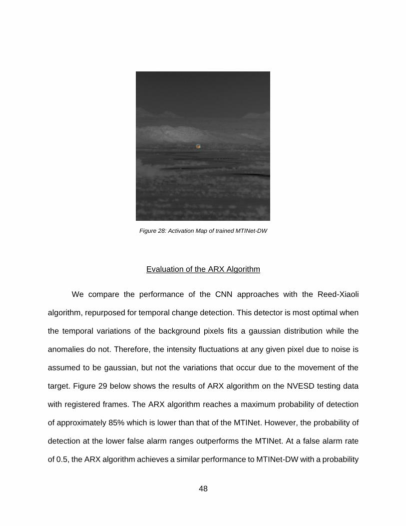
We further investigate the networks ability to localize a moving target using guided
backpropagation to draw a heatmap of the activations produced by the last convolutional
layer. Using the same process described in Experiment Analysis, we generate a heatmap
using a block of five frames from the testing set. Figure 28 below shows the generated
heatmap overlayed on the middle frame from the block of five frames. The heatmap
shows that the network is able to accurately localize the target while producing almost no
response to the surrounding clutter.
48
Figure 28: Activation Map of trained MTINet-DW
Evaluation of the ARX Algorithm
We compare the performance of the CNN approaches with the Reed-Xiaoli
algorithm, repurposed for temporal change detection. This detector is most optimal when
the temporal variations of the background pixels fits a gaussian distribution while the
anomalies do not. Therefore, the intensity fluctuations at any given pixel due to noise is
assumed to be gaussian, but not the variations that occur due to the movement of the
target. Figure 29 below shows the results of ARX algorithm on the NVESD testing data
with registered frames. The ARX algorithm reaches a maximum probability of detection
of approximately 85% which is lower than that of the MTINet. However, the probability of
detection at the lower false alarm ranges outperforms the MTINet. At a false alarm rate
of 0.5, the ARX algorithm achieves a similar performance to MTINet-DW with a probability

49
of detection of about 75%. However, at a false alarm rate of 0.1, the algorithm reaches a
probability of detection of 60% which is higher than both MTINet-CC and MTINet-DW by
about 10%.
Figure 29: ARX Algorithm results on NVESD testing data with registered frames
Combining MTINet and the ARX Algorithm
Based on the results in Evaluation of the ARX Algorithm, we observed that the
trained CNN’s are better at finding more targets at higher false alarm rates but the ARX
detector can find more targets at a lower false alarm rate. Therefore, we utilize the ARX
algorithm concurrently with the MTINet-DW to combine the best of both approaches, i.e.
the ability of the ARX algorithm to find more targets at low FAR with the ability of the
MTINet-DW to find more targets overall. We do so by normalizing and merging the output
detections then identifying likely accurate detections versus false alarms using the
normalized confidence scores. Figure 30 below shows the effectiveness in combining the
two algorithms on the NVESD testing data with registered frames.

50
Figure 30: Combined MTINet-DW and ARX algorithm results on the NVESD testing data with registered frames
Figure 31 below compares the ROC curves of the combined algorithms versus the
individual performance of each on the NVESD testing set with registered frames. We see
that the combination bridges the gap between the 0 to 0.5 false alarm rate range and then
continues to perform similarly to MTINet-DW above that range.
Figure 31: Comparison of MTINet-DW, the ARX algorithm, and their combination on the NVESD testing set

51
CHAPTER FIVE: CONCLUSION AND FUTURE WORK
In comparison to experiments done using state-of-the-art networks, the algorithms
proposed here outperform the ability to detect small moving targets in the NVESD
dataset. Using the highest performing variants of each experiment, we can see in Table
3 that MTINet-CC, MTINet-DW, and the combination of MTINet-DW and the Reed-Xiaoli
algorithm all exceed results of the state-of-the-art networks. YOLOv3 achieves the lowest
false alarm rate at its respective maximum probability of detection; however, that
probability of detection is merely 32%. On the original NVESD testing data, MTINet-CC
can detect every target but with a high false alarm rate. At a 0.1 false alarm rate, MTINet-
CC is still able to detect approximately 68% of targets. The performance of MTINet-CC
versus the state-of-the-art networks on the testing set is nearly 50% greater. This
performance increase can likely be attributed to the additional exploitation of temporal
information and an architecture that is built to incorporate that information. We also
believe the modified TCR cost function helps guide our networks to discern target versus
clutter.

52
Table 3: Comparing results of highest performance experiments
Network Maximum PDet FAR @ Maximum
PDet
PDet @ 0.1
FAR
PDet @ 0.5
FAR
YOLOv3 0.32 0.85 0.15 0.27
Mask R-CNN 0.11 1.78 0.03 0.07
MTINet-CC* 0.99 5.0 0.68 0.82
MTINet-CC 0.97 5.0 0.47 0.70
MTINet-DW 0.95 5.0 0.51 0.73
MTINet-DW + ARX 0.95 5.0 0.59 0.75
* Results of MTINet-CC with no sensor movement
When applying simulated sensor movement, we see a major drop in the detection
ability; however, after introducing registration using SURF we’re able to recover that
performance. Figure 32 below shows the performance of MTINet-CC on the unaltered
NVESD testing dataset in comparison with the results of other algorithms with simulated
sensor movement. When introducing simulated sensor movement and registering the
frames, each algorithm can reach closer to the performance on unaltered data. Notably,
the ARX algorithm (which unlike CNN’s, requires no training) also achieved reasonable
results on the testing data. This makes the algorithm quickly deployable into real-time
systems. Therefore, continuing to improve the performance of this algorithm for small
moving target detection is worth pursuing.

53
Figure 32: Comparison of results given simulated sensor movement
Although our algorithms perform well on the NVESD testing set compared to
previous state of the art detectors, we will strive to reduce false alarm rates by an order
of magnitude while further increasing probability of detection. We also believe there is a
need to develop theoretical performance prediction techniques that can provide
meaningful upper bounds on the performance that can be achieved on a particular data
set. Furthermore, the performance of the MTINet must be optimized and evaluated under
more challenging environmental conditions such as smoke, dust, and scintillations
produced by atmospheric turbulence. Beyond, such effects observed in infra-red imagery,
our ultimate goal is to create a network that can generalize to any type of imagery and
accurately detect both stationary and moving objects that are small, medium, or large.
We also aim to further develop the idea of the combination of multiple detection algorithms
for optimal performance.
54
REFERENCES
[1] J. Redmon and A. Farhadi, "YOLOv3: An Incremental Improvement," 2018.
[2] K. He, G. Gkioxari, P. Dollár and R. B. Girshick, "Mask R-CNN," CoRR, vol.
abs/1703.06870, 2017.
[3] I. S. Reed and X. Yu, "Adaptive multiple-band CFAR detection of an optical pattern
with unknown spectral distribution," IEEE Transactions on Acoustics, Speech, and
Signal Processing, vol. 38, no. 10, pp. 1760-1770, 1990.
[4] O. Russakovsky, J. Deng, H. Su, J. Krause, S. Satheesh, S. Ma, Z. Huang, A.
Karpathy, A. Khosla, M. Bernstein, A. C. Berg and L. Fei-Fei, "ImageNet Large Scale
Visual Recognition Challenge," Springer, vol. 115, no. 2015, pp. 211-252, 2015.
[5] T.-Y. Lin, M. Maire, S. Belongie, L. Bourdev, R. Girshick, J. Hays, P. Perona, D.
Ramanan, C. L. Zitnick and P. Dollár, "Microsoft COCO: Common Objects in
Context," Springer, vol. 8693, no. 2014, pp. 740-755, 2014.
[6] "ATR Algorithm Development Data Set," DSIAC.
[7] M. Tan, R. Pang and Q. V. Le, "EfficientDet: Scalable and Efficient Object
Detection," 2020.
[8] S. Qiao, L.-C. Chen and A. Yuille, "DetectoRS: Detecting Objects with Recursive
Feature Pyramid and Switchable Atrous Convolution," 2020.
[9] Z. Huang and J. Wang, "DC-SPP-YOLO: Dense Connection and Spatial Pyramid
Pooling Based YOLO for Object Detection," Information Sciences, vol. 522, 2020.
[10] H. Zhang, C. Wu, Z. Zhang, Y. Zhu, Z. Zhang, H. Lin, Y. Sun, T. He, J. Muller, R.
Manmatha, M. Li and A. Smola, "ResNeSt: Split-Attention Networks," arXiv preprint,
2020.
[11] C.-I. Chang and C. Shao-Shan, "Anomaly detection and classification for
hyperspectral imagery," IEEE Transactions on Geoscience and Remote Sensing,
vol. 40, no. 6, pp. 1314-1325, 2002.
[12] W. Sanghyun, J. Park, J.-Y. Lee and I. S. Kweon, "CBAM: Convolutional Block
Attention Module," in Computer Vision - ECCV 2018, Springer International
Publishing, 2018, pp. 3-19.

55
[13] J. Hu, L. Shen and G. Sun, "Squeeze-and-Excitation Networks," in 2018 IEEE/CVF
Conference on Computer Vision and Pattern Recognition, 2018, pp. 7132-7141.
[14] L. Kaiser, A. N. Gomez and F. Chollet, "Depthwise Separable Convolutions for
Neural Machine Translation," CoRR, vol. abs/1706.03059, 2017.
[15] H. Bay, T. Tuytelaars and L. Van Gool, "SURF: Speeded Up Robust Features," in
Computer Vision -- ECCV 2006, Springer Berlin Heidelberg, 2006, pp. 404-417.
[16] S. Hochreiter and J. Schmidhuber, "Long Short-term Memory," Neural Computation,
vol. 9, pp. 1735-80, 1997.
[17] R. R. Selvaraju, A. Das, R. Vedantam, M. Cogswell, D. Parikh and D. Batra, "Grad-
CAM: Why did you say that? Visual Explanations from Deep Networks," CoRR, vol.
abs/1610.02391, 2016.
[18] J. Long, E. Shelhamer and T. Darrell, "Fully convolutional networks for semantic
segmentation," in 2015 IEEE Conference on Computer Vision and Pattern
Recognition (CVPR), IEEE, 2015, pp. 3431-3440.
[19] B. McIntosh, A. Mahalanobis and S. Venkataramanan, "Infrared Target Detection in
Cluttered Environments by Maximization of a Target to Clutter Ratio (TCR) Metric
using a Convolutional Neural Network," IEEE Transactions on Aerospace and
Electronic Systems, pp. 1-1, 2020.
[20] S. Woo, J. Park, J.-y. Lee and I. S. Kweon, "CBAM: Convolutional Block Attention
Module," CoRR, vol. abs/1807.06521, 2018.
[21] V. Mnih, N. Heess, A. Graves and K. Kavukcuoglu, "Recurrent Models of Visual
Attention," in Advances in Neural Information Processing Systems 2, Curran
Associates, Inc, 2014, pp. 2204-2212.
[22] A. Bochkovskiy, C.-Y. Wang and H.-Y. M. Liao, "YOLOv4: Optimal Speed and
Accuracy of Object Detection," 2020.