Characterizing non-Gaussian clutter and detecting weakgaseous plumes in hyperspectral imagery

James Theiler, Bernard R. Foy, and Andrew M. Fraser

Los Alamos National Laboratory, Los Alamos, NM 87545

ABSTRACT

To detect weak signals on cluttered backgrounds in high dimensional spaces (such as gaseous plumes in hyper-spectral imagery) without excessive false alarms requires that the background clutter be effectively characterized.If the clutter is Gaussian, the well-known linear matched filter optimizes the sensitivity to a given plume signalwhile suppressing the effect of the background clutter. In practice, the background clutter is rarely Gaussian.Here we illustrate non-linear corrections to the matched filter that are optimal for two non-Gaussian cluttermodels and we report on parametric and nonparametric characterizations of background clutter.

Keywords: imagery, hyperspectral, clutter, non-Gaussian, matched filter, chemical plume

1. INTRODUCTION

Imaging spectrometers have been developed and fielded in recent years with high spectral resolution and lowsensor noise. The sensitivity and specificity of these sensors enables them to detect weak signals in clutteredbackgrounds. We are interested in the detection of thin chemical plumes in hyperspectral imagery, and wein particular seek to improve the detection performance by more carefully characterizing the variability of thebackground. We refer to this background as “clutter” to emphasize that it arises not so much from noise in thesensor, but from the unknown layout of whatever materials happen to be in the scene. In particular, the clutteris not something that one would particularly expect to be Gaussian in its distribution. Our interest is twofold:how can we effectively characterize the clutter, and how can we exploit that characterization to better detectplumes?

We begin with a review of the physical formulation of the plume problem in Section 2 where we identifythe linearization that we use as our starting point. This formulation is approximate and does not cover allaspects of the problem, but it allows us to concentrate on one of the most important aspects of the problem:the characterization of the background clutter. In Section 3, we describe a variety of non-Gaussian modelsand statistics that can be used to characterize the clutter. We follow in Section 4 with methods of using thesestatistics and models to effectively detect weak plumes. In Section 5 we describe statistics of actual images, andin Section 6 we conclude with an outline of progress to date and areas for future work.

2. A BRIEF FORMULATION OF THE PLUME PROBLEM

Radiative emission, absorption, and transport through the atmosphere are all nonlinear physical processes.1

The hyperspectral sensor itself will introduce further nonlinearities. Nonetheless, a linear signal-in-noise modelcan often be adequate for modelling the effect of weak plumes with characteristic spectral signatures. Note,however, that if the background clutter is non-Gaussian, then a linear signal model does not necessarily implythat optimal detectors are linear. Physically motivated nonlinear preprocessing steps (e.g., conversion of radianceto brightness temperature, or compensation of atmospheric distortions) can sometimes improve the quality ofthe linear signal-in-noise model.

In each pixel, imaging sensors measure an at-sensor radiance (Lat−sensor). Off-plume contributions toLat−sensor include thermal emission from atmosphere (Lpath) and instrument∗ (Lsensor), and radiance from theground (Lgnd), attenuated by atmospheric absorption (τ atm). That is

Lat−sensor−off−plume = Lpath + Lsensor + Lgndτ atm (1)

Author contact information: {jt,bfoy,afraser}@lanl.gov∗This includes both sensor noise and thermal radiation from the sensor itself onto its own focal plane.

whereLgnd = B(T gnd)εgnd + Ldownwelling(1− εgnd) (2)

and B(T ) is blackbody radiation at temperature T , and εgnd is the ground emissivity. Here, Ldownwelling includesradiation impinging on the ground, a fraction 1− εgnd of which is then reflected back toward the sensor.1

The on-plume radiance includes two other effects: thermal emission from the plume (Lplume), and absorptionof ground emission by the plume (τ plume). Thus:

Lat−sensor = Lpath + Lsensor + Lplumeτ atm︸ ︷︷ ︸

+Lgnd τ plume︸ ︷︷ ︸

τ atm (3)

where the underbraces identify the terms that are due to the presence of a plume. At each wavelength λ, theweak plume transmissivity depends on column density no and the plume signature bλ with

τplumeλ = e−nobλ ≈ 1− nobλ (4)

The vector emissivity is given byεplume = 1− τ plume ≈ nob, (5)

and the radiance due to the plume is given by

Lplume = B(T plume)εplume ≈ B(T plume)nob. (6)

So the full at-sensor radiance, due to the background and the plume, is given by

Lat−sensor ≈[Lpath + Lsensor + Lgndτ atm

]+ nobτ

atm[B(T plume)− Lgnd

](7)

We remark that all quantities vary from pixel to pixel; Lpath and τ atm are usually nearly constant from pixel topixel . All but no are wavelength dependent. We can re-express this as

r = εb+ x (8)

where r = Lat−sensor−on is the radiance measured at the sensor, x =[Lpath + Lgndτ atm

]+ Lsensor is the back-

ground plus noise (what we are calling “clutter”), b is the plume signature, and ε = noτatm

[B(T plume)− Lgnd

]

is the plume “strength” which includes as well as column density, factors for atmospheric transmission, and thethermal contrast between the plume and the ground. The part in square brackets can have a complicated wave-length dependence, but is often constant across the spectrum of interest.2We remark that although r correspondsto what we measure, x corresponds to the clutter that we model.

This fairly simple formulation motivates our interest in studying Eq. (8). Alternative physical derivationsappear in Refs. [2–4]. One may reformulate this expression to incorporate some atmospheric compensation;5 tothe extent that the compensation is accurate, this provides a number of advantages, from simplifying the groundclutter, to reducing the wavelength dependence of the plume strength.

3. CHARACTERIZING CLUTTER

3.1. Gaussian model

A multivariate Gaussian distribution provides a simple model for the clutter, with a number of useful advantages.It is parameterized by a mean µ ∈ Rd and a symmetric positive semi-definite covariance matrix K ∈ Rd×d:

P (x) = (2π)−d/2 |K|−1/2 exp

[

−1

2(x− µ)TK−1(x− µ)

]

(9)

The covariance matrix K = 〈(x − µ)(x − µ)T 〉 expresses the various band-to-band correlations. Given thecovariance matrix, one can identify the directions in Rd in which the clutter has low variance. These low-variance directions are useful because they are more noticeably influenced by weak signals.

Since µ and K are not known a priori, they are usually estimated from the data using

µ̂ = (1/N)∑

i

xi (10)

K̂ = (1/N)∑

i

(xi − µ̂)(xi − µ̂)T (11)

With O(d2) free parameters in the K̂, it is easy to overfit the model, and in particular to underestimate thevariance in the “thin” directions.6

3.2. Non-Gaussian models

3.2.1. Elliptically Contoured (EC) distributions

Manolakis et al.7 proposed using elliptically contoured (EC) distributions to describe hyperspectral data. Onevery useful property that EC distributions share with Gaussian distributions is that they are characterized by acovariance matrix K. In general, an EC distribution is given by a formula

P (x) = (2π)−d/2 |K|−1/2 h(r2) (12)

where r2 = (x− x̂)TK−1(x− µ) is the Mahalanobis distance, and h(r2) is a positive monotonically decreasingfunction of r2. The Gaussian is a special case of the EC family, given by h(r2) = exp(−r2/2).

Since the EC distributions are characterized by a covariance matrix K, they also identify the useful “thin”directions. But by generalizing h(r2), the tails of the distribution can be more faithfully modeled. Marden andManolakis8, 9 recommend a multivariate t-distribution, for which (up to normalization)

h(r2) =

[

1 +1

νr2]−(d+ν)/2

(13)

Here, the parameter ν characterizes the shape of the distribution; as ν → ∞, the distribution approaches aGaussian, but for smaller values of ν the distributions have heavier tails.

3.2.2. Mixture models

Mixture models are distributions that can be expressed as positive linear combinations of other distributions;e.g.,

P (x) = p1P1(x) + p2P2(x) + · · ·+ pKPK(x) (14)

where 0 ≤ pi ≤ 1, and∑

i pi = 1, and each Pi is a normalized probability distribution. In practice, K is usuallysmall (to keep a reasonable number of fitted parameters), and each Pi is a relatively simple distribution, such asa Gaussian or an EC distribution.

Although mixture models are flexible and physically plausible – each mixture component corresponds to aphysically distinct material on the ground – there are costs to using them. Because the likelihood function hassingularities, direct maximum likelihood parameter estimation can fail outright. Even for regularized criterionfunctions, there are not closed form expressions for maxima; simultaneous optimization of all the parametersin all the models can be problematic and iterative procedures such as expectation-maximization are typicallyemployed, but these are not guaranteed to converge to a global optimum. In general, these models have a lot offree parameters, and with limited data to fit them, the variance of the estimates can be unduly large.

But despite these pitfalls, mixture models can still be useful. Funk et al.10 used k-means to fit data to amixture of Gaussians which were effectively assumed not to overlap and found improved detection performance.Marden and Manolakis8 used an expectation-maximization (EM) algorithm to fit multiple EC distribution clus-ters to hyperspectral data. In another paper, Manolakis and Marden11 described a local principal componentsapproach using vector quantization that reduces Euclidean distance errors.

3.2.3. Parzen window model

The Parzen window12 (see also Ref. [13, pp. 164–171]) model provides a nonparametric estimate of the distributionP (x) from a sample of N points taken from that distribution:

P̂ (x) = (1/N)N∑

i=1

σ−dg(|x− xi|

σ) (15)

where g(r) is a “kernel” function that decreases monotonically with increasing r and is normalized so that ad-dimensional radially symmetric distribution has unit volume. A typical choice is

g(r) = (2π)−d/2 exp(−r2/2). (16)

The tail of a Parzen window estimator depends on the kernel g(r), and is Gaussian if the kernels are Gaussian.Thus, this is not a very good way to model fat-tailed distributions.

Also, all directions are only as thin as the Gaussian kernel g(r). To achieve a large dynamic range in thevariance of the distribution in different directions, a very large number of kernels are necessary.

What the Parzen window does have that is potentially advantageous is that it is very data adaptive; in fact,with appropriate choice of σ as a function of N , it can in the N → ∞ limit model virtually any continuousdistribution.

3.2.4. Endmembers

Endmembers14 model the data in a way that does not provide an explicit probability distribution function P (x)for the background clutter. In its simplest form, the endmember model provides a small number k of distinctmaterial spectra, {e1, . . . , ek}, and then asserts that most of the variance in the clutter can be accounted for interms of positive linear combinations of these spectra. That is, each pixel xi is modelled as

xi =

k∑

j=1

pijej + ni (17)

subject to∑

j pij = 1. Here, 0 ≤ pij ≤ 1 is interpreted as the abundance of the jth material in the ith pixel,and ni is the residual which is usually modelled as some kind of Gaussian noise process.

The endmembers are sometimes referred to as “interferers” and detection in a scene that is modeled byendmembers is usually achieved by first “projecting out” the subspace spanned by the endmembers, and thenemploying an ordinary matched filter on the lower dimensional (d−k) space that is orthogonal to the endmembers.See, for instance, Refs. [15, 16].

4. LINEAR AND NONLINEAR PLUME DETECTORS

Usually detector performance is graded probabilistically in terms of a receiver operating characteristic (ROC)that describes the trade off between detection probability and false alarm rate. Given probabilistic descriptionsof the possible signals, i.e., PH0

and PH1for measurements of a pixel with and without a plume respectively and

a radiance measurement r, the familiar likelihood ratio test is optimal.13, 17 Here the test is given by

H =

H0 L(r) < γ

H1 L(r) ≥ γ(18)

where

L =PH1

(r)

PH0(r)

(19)

is the likelihood ratio. The threshold γ determines a single point on the ROC curve, and is often specified toyield a particular false alarm rate.

(a) (b) (c)

−1 −0.5 0 0.5 1

1

1.2

1.4

1.6

1.8

2

−1 −0.5 0 0.5 1

1

1.2

1.4

1.6

1.8

2

−1 −0.5 0 0.5 1

1

1.2

1.4

1.6

1.8

2

Figure 1. Decision boundaries of the GLRT detector. The lines follow level sets of L(r) from Eq. (21). A whiteneddistribution in d = 2 dimensional space is centered at the origin; these contours correspond to detection of a plumewith signature b = [0, 1] in the vertical direction. (a) A Gaussian distribution leads to linear contours, correspondingto constant values of the matched filter q = K−1b. Since this is whitened space, K = I and q = b and the contoursare horizontal lines. (b) A leptokurtic (fat-tailed) distribution is provided by a multivariate t-distribution with ν = 5.0.Here the detection contours bend away from the origin, relative to how they behave for a Gaussian distribution. (c) Aplatykurtic (thin-tailed) distribution is given by P (r) = C exp(−|r|4) where C is just a normalization constant. Here, thecontours bend back toward the origin.

When probabilistic descriptions are unavailable or incomplete, designing optimal or even good detectors ismore challenging. In this section, we will describe and illustrate a variety of detectors and discuss conditions forwhich they are optimal or useful.

If the plume strength ε were known, then the likelihood ratio could be applied directly, and the optimal testfor plume versus no-plume would be in terms of the ratio

L(r) =P (r− εb)

P (r). (20)

But since ε is unknown, this approach needs to be modified. Two approaches for doing this follow.

4.1. Generalized Likelihood Ratio Test (GLRT)

To treat the case of unknown signal strength, Kelly18 introduced the generalized likelihood ratio test (GLRT).The idea behind the GLRT is to replace all nuisance parameters (such as ε) with their maximum likelihoodestimates. Here,

L(r) =maxε P (r− εb)

P (r). (21)

Fig. 1 shows contours of this likelihood ratio for three different distributions P (x): one is Gaussian, one is fat-tailed, and one is thin-tailed. The GLRT is not known in general to be optimal, but Scharf and Friedlander19

have shown that it does possess optimality properties in some special cases (in particular, when the distributionis Gaussian).

4.1.1. GLRT for Gaussian

If P (r) is Gaussian, then the formula in Eq. (21) can be used directly. We will for simplicity assume µ = 0 andthat K is known. Then P (r) = C exp(− 1

2rTK−1r) for constant C = (2π)−d/2|K|−1/2, and the GLRT becomes

L(r) =maxε C exp

[− 12 (r− εb)TK−1(r− εb)

]

C exp[− 12r

TK−1r]

= maxεexp

[

−1

2(r− εb)TK−1(r− εb) +

1

2rTK−1r

]

(22)

(a) (b) (c)

−1 −0.5 0 0.5 1

1

1.2

1.4

1.6

1.8

2

−1 −0.5 0 0.5 1

1

1.2

1.4

1.6

1.8

2

−1 −0.5 0 0.5 1

1

1.2

1.4

1.6

1.8

2

Figure 2. Decision boundaries for the local derivative detector. This figure is the same as Fig. 1, except that it usesthe local derivative method instead of the generalized likelihood ratio test. The lines follow solutions of Eq. (28) (a). AGaussian distribution leads to linear contours. The contours in this figure (like those in Fig. 1) are not calibrated, soprovide information only on the “shape” of the contours. (b) A leptokurtic (fat-tailed) distribution leads to detectioncontours that bend away from the origin. (c) A platykurtic (thin-tailed) distribution leads to contours that bend backtoward the origin.

Taking the logarithm,

`(r) = logL(r) = maxε

(

− (r− εb)TK−1(r− εb) + rTK−1r

)

= maxε

(

εbTK−1r+ εrTK−1b− ε2bTK−1b

)

(23)

The maximum occurs at

ε =bTK−1r

bTK−1b(24)

which leads to

`(r) =

(bTK−1r

)2

bTK−1b. (25)

Recall that this derivation assumed that the Gaussian distribution P (r), and in particular the covariance K,is known precisely. In practice, K must be estimated from data. The natural choice, advocated by Reed et al.,20

is to use the estimator for K̂ in Eq. (11) in place of the exact K in Eq. (25). In Kelly’s derivation,18 a morecareful approach, in which µ̂, K̂, and ε are simultaneously estimated in the numerator of Eq. (21), leads to adiscriminant function of the form

|bT K̂−1r|2

bT K̂−1b(

1 + 1N r

T K̂−1r) , (26)

although a later publication21 suggested that the simpler matched filter in Eq. (25) was more practical.

Note that Eq. (25) implies that the contours of constant likelihood ratio occur at constant values of qT r whereq = K−1b. These are the contours of the optimal linear matched filter that one can obtain more simply bymaximizing a signal to clutter ratio. Although we can derive the filter without appealing to Gaussian distributionsat all, if the data are not Gaussian, the probabilistic performance of the detector may not be optimal.

4.2. Local derivative method (small ε limit)

Since we do not know the magnitude of ε, we cannot use the likelihood ratio in Eq. (20). In the GLRT, we usethe maximum likelihood estimate of ε, but that can lead to values of ε that might not accord with what is known

about the physics of the plume. We will consider here the situation in which we don’t know the magnitude of ε,but we do know that it is small. We begin with the likelihood ratio in Eq. (20), and take the small ε limit.

L(r) =P (r− εb)

P (r)≈

P (r)− εb · ∇P (r)

P (r)(27)

Since we are interested in contours of constant L(r), these occur when

b · ∇P (x)

P (x)= c (28)

for some constant c which depends on p. We remark that the constant c is like the threshold γ in Eq. (18),and needs to be “calibrated” against, for instance, a desired false alarm rate. Fig. 2 illustrates what contoursspecified by Eq. (28) look like for three different distributions P (x).

4.2.1. Gaussian P (r)

Note that for Gaussian P (r) = C exp(− 12r

TK−1r), we have

b · ∇P

P= b · ∇(logP ) = b · ∇

(

logC −1

2rTK−1r

)

= bTK−1r (29)

which implies that contours are along lines of constant qT r where q = K−1b.

5. STATISTICS OF HYPERSPECTRAL IMAGERY

It is evident by inspection that background clutter in hyperspectral imagery is non-Gaussian. To illustrate this,we provide two small 128×128 chips from AVIRIS22, 23 dataset f970620t01p02 r03 sc01; this is a reflectanceimage over the Moffett Field area in California. One chip is from a predominantly rural area, and the otheris an urban scene. In both cases, as seen in Fig. 3, scatterplots of the first two principal components of thehyperspectral image show decidedly non-Gaussian distributions.

But quantitative characterization of multivariate distributions (especially the high-dimensional distributionsin hyperspectral imagery) is difficult – this is the curse of dimensionality problem – so we characterize distribu-tions of various one-dimensional projections of the data.

5.1. Mahalanobis distances

Given a covariance matrixK, the Mahalanobis distance is Euclidean distance in the whitened space: in particular,the Mahalanobis distance between two points r1 and r2 is given by

r2 = (r1 − r2)TK−1(r1 − r2). (30)

If the data were Gaussian, the Mahalanobis distances would have a chi-squared distribution with d degrees offreedom, where d is the dimension of the space (i.e., the number of channels in the hyperspectral imagery). Formore general EC distributions, the distribution of Mahalanobis distances will be different. For real hyperspectralimages, the distribution of Mahalanobis distances is usually reported to be fat-tailed,7 and we see that aswell in Fig. 4. If the data are distributed according to the multivariate t-distribution in Eqs. (12,13), then theMahalanobis distances are distributed with an Fd,ν distribution.

8

5.2. Distribution of matched-filter projections

A more direct alternative to Mahalanobis distances are projections of the data onto one-dimensional axes. Thisprovides scalars whose distributions can be characterized by statistics, such as the kurtosis, which is defined

κq =〈(qT r− qT µ̂)4〉

〈(qT r− qT µ̂)2〉2(31)

Unlike the Mahalanobis distances, direct projections provide statistics which do not depend on estimating thecovariance matrix. The projection provides a different set of scalars for each projection direction b. As well asproviding a statistic that is direction-dependent, this approach provides a statistic that is particularly appropriatefor characterizing the “important” directions of a distribution – these are the directions that a matched filterwould employ in a linear plume detection scenario.

(a) (b) (c)

−2 −1 0 1 2 3

x 104

−2

−1

0

1

2x 10

4

PC 1

PC

2

(d) (e) (f)

−10 −8 −6 −4 −2 0 2

x 104

−1

−0.5

0

0.5

1

1.5

2x 10

4

PC 1P

C 2

Figure 3. Two small 128×128 chips from an AVIRIS hyperspectral image. The upper panels (a-c) correspond to a chipfrom a mountainous part of the scene, while the lower panels (d-f) correspond to an image of the urban area. Here,(a,d) are images of the first principal component, and (b,e) are images of the second principal component. Scatterplotsof the first and second principal components appear in (c,f). It is evident in these scatterplots that the data are not welldescribed as Gaussian.

5.2.1. Finite sample effects in estimates of kurtosis and variance

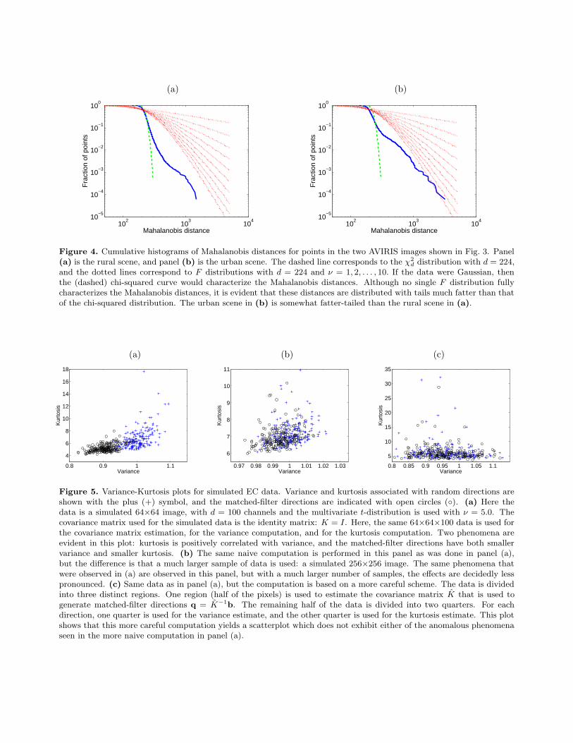
For an EC distribution, the kurtosis will be the same for all projections. We do know that the variance of thedata along a projection does vary with direction; indeed, the variance in direction b is given by bTKb. So oneway to investigate whether the kurtosis varies with direction is to test whether it varies with variance. For agiven data set, we examined both the kurtosis and the variance in a number of random directions. Since we areparticularly interested in directions associated with matched filters, we will for every direction b also considerthe matched-filter direction q = K−1b. If we do this for simulated data from an EC distribution, we shouldfind that the kurtosis is independent of direction, and therefore, independent of variance. Fig. 5(a) shows whatthis plot looks like when the experiment is performed naively, on a dataset with a small number of pixels. Itappears that there is a correlation between variance and kurtosis, with the low-variance directions exhibitinglow kurtosis. That this is a finite-sample effect is evident in Fig. 5(b) which shows that for a data set with alot more samples, the effect is much smaller. To alleviate this finite-sample bias, we perform a more carefulcomputation, in which the hyperspectral image is partitioned into three disjoint regions. The first region is usedto estimate the covariance matrix, the second region is used for estimating variance, and the third region is usedfor estimating kurtosis. As Fig. 5(c) shows, this more careful approach does not show a correlation betweenvariance and kurtosis for simulated EC data.

5.2.2. Kurtosis and variance in real hyperspectral imagery

In investigating whether such a correlation exists in real data, we will henceforth use the more careful approachwith the partition of the image into disjoint regions. In Fig. 6, we compute kurtosis-variance plots for the two

(a) (b)

102

103

104

100

10−1

10−2

10−3

10−4

10−5

Mahalanobis distance

Fra

ctio

n of

poi

nts

102

103

104

100

10−1

10−2

10−3

10−4

10−5

Mahalanobis distance

Fra

ctio

n of

poi

nts

Figure 4. Cumulative histograms of Mahalanobis distances for points in the two AVIRIS images shown in Fig. 3. Panel(a) is the rural scene, and panel (b) is the urban scene. The dashed line corresponds to the χ2

d distribution with d = 224,and the dotted lines correspond to F distributions with d = 224 and ν = 1, 2, . . . , 10. If the data were Gaussian, thenthe (dashed) chi-squared curve would characterize the Mahalanobis distances. Although no single F distribution fullycharacterizes the Mahalanobis distances, it is evident that these distances are distributed with tails much fatter than thatof the chi-squared distribution. The urban scene in (b) is somewhat fatter-tailed than the rural scene in (a).

(a) (b) (c)

0.8 0.9 1 1.1

4

6

8

10

12

14

16

18

Variance

Kur

tosi

s

0.97 0.98 0.99 1 1.01 1.02 1.03

6

7

8

9

10

11

Variance

Kur

tosi

s

0.8 0.85 0.9 0.95 1 1.05 1.1

5

10

15

20

25

30

35

Variance

Kur

tosi

s

Figure 5. Variance-Kurtosis plots for simulated EC data. Variance and kurtosis associated with random directions areshown with the plus (+) symbol, and the matched-filter directions are indicated with open circles (◦). (a) Here thedata is a simulated 64×64 image, with d = 100 channels and the multivariate t-distribution is used with ν = 5.0. Thecovariance matrix used for the simulated data is the identity matrix: K = I. Here, the same 64×64×100 data is used forthe covariance matrix estimation, for the variance computation, and for the kurtosis computation. Two phenomena areevident in this plot: kurtosis is positively correlated with variance, and the matched-filter directions have both smallervariance and smaller kurtosis. (b) The same naive computation is performed in this panel as was done in panel (a),but the difference is that a much larger sample of data is used: a simulated 256×256 image. The same phenomena thatwere observed in (a) are observed in this panel, but with a much larger number of samples, the effects are decidedly lesspronounced. (c) Same data as in panel (a), but the computation is based on a more careful scheme. The data is dividedinto three distinct regions. One region (half of the pixels) is used to estimate the covariance matrix K̂ that is used togenerate matched-filter directions q = K̂−1b. The remaining half of the data is divided into two quarters. For eachdirection, one quarter is used for the variance estimate, and the other quarter is used for the kurtosis estimate. This plotshows that this more careful computation yields a scatterplot which does not exhibit either of the anomalous phenomenaseen in the more naive computation in panel (a).

(a) (b)

10−6

10−4

10−2

100

102

2

3

4

5

6

7

8

9

Variance

Kur

tosi

s

10−6

10−4

10−2

100

5

10

15

20

25

30

35

40

Variance

Kur

tosi

s

Figure 6. Kurtosis-variance plots for the (a) rural and (b) urban scenes of the AVIRIS data described in Fig. 3. Varianceand kurtosis associated with random directions are shown with the plus (+) symbol, and the matched-filter directionsare indicated with open circles (◦). It is not surprising that the variance would be much smaller for the matched-filter directions, indeed many orders of magnitude smaller, since the matched-filter directions are explicitly designed tominimize the magnitude of the background clutter. But what is striking is that the kurtosis in the low-variance matched-filter directions is much smaller than the kurtosis in the higher-variance random directions; indeed, the matched-filterdirections exhibit a kurtosis roughly equal to three, the same value exhibited by a Gaussian distribution. Also, as observedin Fig. 4, the urban scene in (b) exhibits considerably fatter tails (more kurtosis) than does the rural scene in (a).

(a) (b) (c)

102

103

104

100

10−1

10−2

10−4

10−3

10−5

Mahalanobis distance

Fra

ctio

n of

poi

nts

100

10−2

10−4

10−6

10−8

0

20

40

60

80

100

Variance

Kur

tosi

s

Figure 7. (a) Broadband image of the Hyperion image, obtained by adding the signal in all the channels. Some evidenceof striping can be seen even in this broadband image. Particular channels show the effect much more strikingly. (b)Mahalanobis histogram, like those shown in Fig. 4 indicates a very fat-tailed distribution. (c) Kurtosis-variance plotexhibits very large kurtosis values for the random directions, although the match-filter directions show, by comparison,much smaller kurtosis values.

AVIRIS datasets, and find that there is a strong correlation. Even accounting for the finite sample effects, lowervariance directions in these datasets exhibit smaller kurtosis (and are more Gaussian) than random directionswhich tend to have higher variance. This suggests that the elliptically contoured models do not adequatelycapture this aspect of the tails of the distributions of real data.

5.2.3. Remark on image artifacts

The effect seen in the AVIRIS data has been observed in other hyperspectral datasets as well. We exhibit herea dataset of the Collembally Irrigation Area in Australia, taken from the spaceborne Hyperion sensor.24

Fig. 7 illustrates this Mahalanobis and Kurtosis-variance analysis of the original Hyperion data. Evidence fora strongly leptokurtic (heavy-tailed) distribution is seen in both the Mahalanobis histogram and in the kurtosis-

(a) (b) (c)

102

103

104

100

10−1

10−2

10−3

10−4

10−5

Mahalanobis distanceF

ract

ion

of p

oint

s

100

10−2

10−2

10−6

10−8

10−4

1

2

3

4

5

6

7

Variance

Kur

tosi

s

Figure 8. (a) Broadband image of the cleaned-up Hyperion image. Comparison to Fig. 7(a) shows that this is a sub-imageof the original; the sub-image was chosen to avoid some of the artifacts that were evident in the original. Also, some ofthe more problematic bands in the original (specifically, bands 94, 99, 116, 168, 169, 190, and 203) were eliminated in thisimage. (b) The Mahalanobis histogram shows that the fat-tail seen in Fig. 7(b) is hardly evident in the cleaned-up image.(c) Kurtosis-variance plot shows that the kurtosis for random directions (+) in the cleaned-up image is considerablysmaller than for the original image, as seen in Fig. 7(c). In fact, in this data, the kurtosis for the random directionaverages near 3.0, the kurtosis of a Gaussian distribution. The kurtosis for the matched-filter directions are much moretightly clustered around the Gaussian kurtosis value of 3.0.

variance plot. However, a cursory examination of the data indicates that there are a number of imaging artifacts.Indeed some of these can be seen in Fig. 7(a) in the form of vertical stripes.

By eliminating some of the problematic spectral bands, and by choosing a chip of the image that avoidsthe edges of the data and some of the striping artifacts, a “cleaned-up” dataset was produced. This is a veryunsophisticated approach to data clean-up, but it illustrates the point, evident in Fig. 8, that cleaning up animage can go a long way to eliminating, or at least reducing, the fat-tailed distribution of the data.

6. CONCLUSION

We observe, as others have (e.g., Ref. [7]), that hyperspectral image data is not always well-modelled as Gaussian,and usually exhibits heavier tails than Gaussian. In the presence of non-Gaussian clutter, the optimal detectors ofweak signatures were shown to be nonlinear. A local derivative method was introduced as a small ε alternative tothe generalized likelihood ratio test (GLRT). The local derivative method is equivalent to the GLRT for Gaussiandata, and gives results for non-Gaussian distributions that are qualitatively similar to the GLRT.

Our investigation of the non-Gaussian characteristics of hyperspectral imagery emphasized distributions ofprojected data, instead of Mahalanobis distances. This enabled us to compare the structure of the hyperspectralclutter in different directions, and we found that projections on directions with small variance are closer toGaussian than projections on directions with larger variance. Since matched-filter directions have low varianceby design, we might expect matched-filter detectors to be more nearly optimal than would be predicted byfat-tailed models of clutter in hyperspectral imagery.

These results contrast with those of McVey et al.,25 who report that false positives produced by a matchedfilter are distributed with fatter-than-Gaussian tails. Similar results are reported by Manolakis et al.7 Perhapsimage artifacts, as depicted in Fig. 7 and Fig. 8, play a role in the discrepancy between these reports and ourobservations. It is also possible that actual gaseous plume signatures are not well-modeled as “random” directions(i.e., there may be systematic correlation between the target and the ground scene signatures).

ACKNOWLEDGMENTS

We are grateful to Chris Borel, Herb Fry, Brian McVey, and Kevin Mitchell for useful discussions. This workwas supported by the Laboratory Directed Research and Development (LDRD) program at Los Alamos.

REFERENCES

1. J. Schott, Remote Sensing: the Image Chain Approach, Oxford University Press, New York, 1997.

2. B. R. Foy, R. R. Petrin, C. R. Quick, T. Shimada, and J. J. Tiee, “Comparisons between hyperspectralpassive and multispectral active sensor measurements.,” Proc. SPIE 4722, pp. 98–109, 2002.

3. A. Hayden, E. Niple, and B. Boyce, “Determination of trace-gas amounts in plumes by the use of orthogonaldigital filtering of thermal-emission spectra,” Applied Optics 35, pp. 2803–2809, 1996.

4. S. J. Young, “Detection and quantification of gases in industrial-stack plumes using thermal-infrared hyper-spectral imaging,” Tech. Rep. ATR-2002(8407)-1, The Aerospace Corporation, 2002.

5. S. J. Young, B. R. Johnson, and J. A. Hackwell, “An in-scene method for atmospheric compensation ofthermal hyperspectral data,” J. Geophys. Res. Atm. 107, pp. 4774–4774, 2002.

6. P. V. Villeneuve, H. A. Fry, J. Theiler, B. W. Smith, and A. D. Stocker, “Improved matched-filter detectiontechniques,” Proc. SPIE 3753, pp. 278–285, 1999.

7. D. Manolakis, D. Marden, J. Kerekes, and G. Shaw, “On the statistics of hyperspectral imaging data,” Proc.SPIE 4381, pp. 308–316, 2001.

8. D. B. Marden and D. Manolakis, “Modeling hyperspectral imaging data,” Proc. SPIE 5093, pp. 253–262,2003.

9. D. B. Marden and D. Manolakis, “Using elliptically contoured distributions to model hyperspectral imagingdata and generate statistically similar synthetic data,” Proc. SPIE 5425, pp. 558–572, 2004.

10. C. C. Funk, J. Theiler, D. A. Roberts, and C. C. Borel, “Clustering to improve matched filter detection ofweak gas plumes in hyperspectral imagery,” IEEE Trans. Geoscience and Remote Sensing 39, pp. 1410–1420,2001.

11. D. Manolakis and D. Marden, “Dimensionality reduction of hyperspectral imaging data using local principalcomponents transforms,” Proc. SPIE 5425, pp. 393–401, 2004.

12. E. Parzen, “On estimation of probability density function and mode,” Ann. Math. Stat. 33, pp. 1065–1076,1962.

13. R. O. Duda, P. E. Hart, and D. G. Stork, Pattern Classification, John Wiley & Sons, New York, 2001.

14. J. W. Boardman, “Automating spectral unmixing of AVIRIS data using convex geometry concepts,” inSummaries of the Fourth Annual JPL Airborne Geoscience Workshop, R. O. Green, ed., pp. 11–14, 1994.

15. J. C. Harsanyi and C.-I. Chang, “Hyperspectral image classification and dimensionality reduction: andorthogonal subspace projection approach,” IEEE Trans. Geoscience and Remote Sensing 32, pp. 779–785,1994.

16. J. J. Settle, “On the relationship between spectral unmixing and subspace projection,” IEEE Trans. Geo-

science and Remote Sensing 34, pp. 1045–1046, 1996.

17. K. Fukunaga, Introduction to Statistical Pattern Recognition, Academic Press, San Diego, second ed., 1990.

18. E. J. Kelly, “An adaptive detection algorithm,” IEEE Trans. Aerospace and Electronic Systems 22, pp. 115–127, 1986.

19. L. L. Scharf and B. Friedlander, “Matched subspace detectors,” IEEE Trans. Signal Processing 42, pp. 2146–2156, 1994.

20. I. S. Reed, J. D. Mallett, and L. E. Brennan, “Rapid convergence rate in adaptive arrays,” IEEE Trans.

Aerospace and Electronic Systems 10, pp. 853–863, 1974.

21. F. C. Robey, D. R. Fuhrmann, E. J. Kelly, and R. Nitzberg, “A CFAR adaptive matched filter detector,”IEEE Trans. Aerospace and Electronic Systems 28, pp. 208–216, 1992.

22. G. Vane, R. O. Green, T. G. Chrien, H. T. Enmark, E. G. Hansen, and W. M. Porter, “The AirborneVisible/Infrared Imaging Spectrometer (AVIRIS),” Remote Sensing of the Environment 44, pp. 127–143,1993.

23. AVIRIS Free Standard Data Products, Jet Propulsion Laboratory (JPL), National Aeronautics and SpaceAdministration (NASA). http://aviris.jpl.nasa.gov/html/aviris.freedata.html.

24. http://eo1.gsfc.nasa.gov/Technology/Hyperion.html.

25. B. McVey, T. Burr, and H. Fry, “Distribution of chemical false positives for hyperspectral image data,”Tech. Rep. LA-CP-02-521, Los Alamos National Laboratory, 2003.