Design and Optimization of a New Stator for the Transonic ... AND OPTIMIZATION OF A NEW STATOR FOR...

DESIGN AND OPTIMIZATION OF A NEW STATOR FOR THE TRANSONIC COMPRESSOR RIG AT TU DARMSTADT

F. Bakhtiari1, F. Wartzek1, S. Leichtfuß1, H.-P. Schiffer1, G. Goinis2, E. Nicke2

1Technische Universität Darmstadt, Germany (GLR) Institute of Gas Turbines and Aerospace Propulsion, Otto-Berndt-Straße 2, 64287 Darmstadt, Germany

2German Aerospace Center (DLR), Institute of Propulsion Technology,

Linder Hoehe, 51147 Cologne, Germany

Abstract The Institute of Gas Turbines and Aerospace Propulsion at the Technische Universität Darmstadt operates a transonic compressor test rig that represents the typical front-stage of a turbofan high-pressure compressor. The baseline stator was designed in the 1990s and the geometry no longer conforms to modern turbo machine designs and trends in premature flow separation. This paper presents the modification of the current baseline stator design and the development of a new 3D stator using an automated multi-objective optimization process with more than 70 free design variables, two objective functions and 3D CFD for different operating points. The result of the optimization was a new stator design with distinct 3D features, which shows no signs of flow separation across the whole operation range and homogenous angular distribution of outflow. The isentropic efficiency could thus be increased by a maximum of 2.5% while maintaining the same range of operability. As part of this process, the geometric parameters with the most significant impact on aerodynamic behaviour are identified. Therefore, the focus is on the aerodynamic influence of 3D features such as bow and sweep, which primarily reduce total pressure loss. The presented research work was done in a joint collaboration between DLR Institute of Propulsion Technology and Technische Universität Darmstadt (GLR).

NOMENCLATURE AR aspect ratio ADP aerodynamic design point CDF computational fluid dynamics DLR Deutsches Zentrum für Luft- und Raumfahrt (German Aerospace Center) DTC Darmstadt Transonic Compressor D/C direct current ER expansion ratio LE leading edge TE trailing edge TRACE Turbomachinery Research Aerodynamic Computational Environment (flow solver) OP operating point RANS Reynolds-Averaged Navier-Stokes RPM revolutions per minute TUD Technische Universität Darmstadt CDA control diffusion airfoil VIGV Variable-Inlet-Guide-Vanes 𝑐 axial chord length [mm] 𝑐! absolute velocity at stator inlet [m/s] 𝑐! absolute velocity at stator outlet [m/s] 𝐷!"# maximum profile thickness [mm] 𝑚 mass flow rate [kg/s] 𝜋!"! total pressure ratio [-] 𝜂!" isentropic efficiency [-] n rotational speed [1/min]

𝛽!" outflow angle [°] 𝛽! stagger angle [°] 𝛽! leading edge angle [°] 𝛽! trailing edge angle [°] 𝑝!! total pressure at stator inlet [Pa] 𝑝!! total pressure at stator outlet [Pa] 𝑝!"#"! static pressure at stator inlet [Pa] 𝑝!"#! dynamic pressure at stator inlet [Pa] 𝑠 chord length [mm] 𝜔 total pressure loss [-] 𝑓 fitness function 𝐹 global blade force [N] ℎ!"# relative duct height [-] 𝑥!"#$ position of maximum thickness [mm] 𝑟!" leading edge radius [mm]

1. INTRODUCTION This paper presents the multi-objective optimisation of a highly loaded stator, which is part of the baseline configuration of the Darmstadt Transonic Compressor (DTC) at TUD. This baseline configuration is used for fundamental research and validation of numerical methods. The baseline stator geometry does not conform to modern turbo machine designs and trends in premature flow separation near hub and shroud. These separations exist over a wide operating range, which have been

Deutscher Luft- und Raumfahrtkongress 2015DocumentID: 370225

1

demonstrated in previous studies by Hergt et al. [4]. The highly loaded stator is challenging for numerical simulations, as the accurate calculation of separation onset and reattachment is still difficult using “classical" RANS with isotropic turbulence models. Separation of the stator increases the complexity of the simulations unnecessarily, especially when the focus should be on the rotor flow. This paper is motivated by enlarging the test case to a modern stator geometry, which shows no signs of flow separation and a homogenous angular distribution of outflow in a wide range of operation. This is preferred for two reasons. First, the optimized design should deliver the same deflection but with reduced deviation (the investigated stator (Stator 1) was designed for an axial outflow). Second, the instrumentation of the stage is designed with a fixed angle along the span, thus guaranteeing optimum flow conditions for the instrumentation. Many attempts have been made to eliminate corner stall while reducing endwall losses. Breugelmans et al. [5] and Sasaki et al. [6] clarified the positive effects of lean and sweep in a linear compressor cascade. Weingold et al. [7] investigated bowed stators in a three-stage compressor, with lean on both endwalls, and reported a one percent increase in overall efficiency and elimination of corner stall. This research showed that reduction of endwall losses requires a 3D stator geometry with distinct 3D features, such as bow and sweep. It is almost impossible to design an optimum stator that has these distinct 3D features using analytical tools. Constantly increasing computational capacity allows automated CFD optimization to become an essential part of modern aerodynamic compressor design. Geometry design tools and CFD solvers are arranged in a process chain and coupled with an optimization algorithm. This modern design method is applied to improve the baseline stator geometry [8, 15].

A brief overview of the test case and the optimization setup is presented below.

2. TEST CASE

FIGURE 1. Diagram of the Darmstadt transonic

compressor [3]

The Darmstadt Transonic Compressor (DTC) at TUD is used for this study. The test rig was built and designed in cooperation with MTU Aero Engines (Munich) and

commissioned in 1994. The rig is operated in an open circuit where air is sucked in then released back into the atmosphere. A throttle is used to control compressor back pressure. The basic diagram of the compressor test facility and infrastructure is displayed in Figure 1. The facility is operated as a single or 1.5 stage transonic compressor, with various rotor and stator configurations and possible flow path modifications, for example, casing treatments and inflow distortions. The single stage configuration consists of a rotor and a stator. The 1.5 stage configuration is extended by introducing Variable-Inlet-Guide-Vanes (VIGV). The facility design parameters are summarized in Table 1. The facility is driven by an 800 kW D/C drive. Shaft speed and power are monitored using a torque meter. A gearbox is used to alter the speed of the D/C drive, which can achieve up to 21,000 rpm. Further details of the rig design can be found in Schulze et al. [3].

Pressure Ratio 1.5

Corrected Mass Flow Rate 16 kg/s

Max. Shaft Speed 21,000 rpm

Power 800 kW

Rotor Blades 16

Stator Blades 29

TAB 1. Compressor design parameters

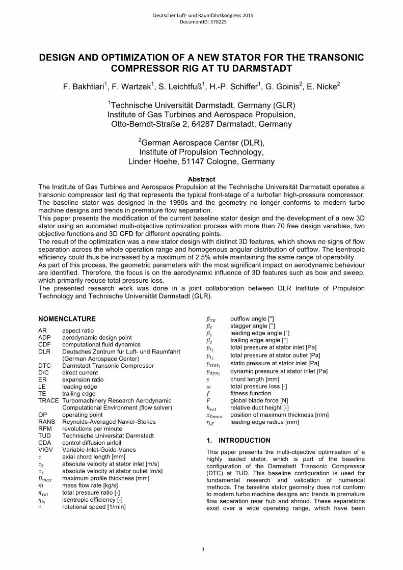
2.1. Compressor Stage / Test section

FIGURE 2. Compressor test rig cross-section

The compressor stage (Figure 2) is the baseline design from 1994 and consists of rotor, stator and outlet strut. The computational domain is also shown. To simplify the numerical setup, the spinner region of the rotor is only partially meshed. The outlet struts are ignored as the upstream effect is relatively small. The inlet boundary layer profile upstream of the stage is measured using a boundary layer probe. This profile is used for the numerical boundary conditions. The rotor (Rotor 1) is designed with radially stacked CDA profiles (controlled diffusion airfoils) and is milled from one piece of titanium (BLISK - bladed disk). Further details of the rotor design can be found in Schulze et al [3]. The investigated stator is also designed with radially

Inlet Throttle : 0Settling chamber : 1

Intake with mass flow measurement : 2Test compressor : 3

Torquemeter : 4Gearbox : 5

800kW DC-Drive : 6

1 2 3 4 5 6

0

computational domain

Rotor Stator 5 outlet struts

Deutscher Luft- und Raumfahrtkongress 2015

2

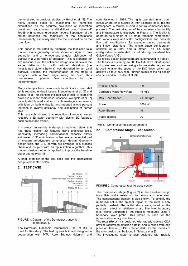
stacked CDA profiles without any 3D features. Figure 3 is a picture of the stator that shows an oil flow visualization on the profile surface. The highly loaded stator has great deficits in form of a large flow separation at hub and shroud.

FIGURE 3. Baseline geometry, separation near hub and

shroud

3. NUMERICAL SETUP A numerical grid is generated that includes one rotor (red) and one stator (blue) passage (Figure 2). For this optimization, a structured grid with approximately 1.5 million cells with an OCH topology is used. The rotor tip gap is modelled with 7 cell layers. All boundary layers are resolved using wall functions. The 𝑦! values are in the range of 35 to 85. The mixing plane is located between the rotor exit and the stator inlet. An overview of basic mesh quality parameters is given in Table 2.

Nodes Min angle ERmax ARmax

Rotor 843k 27.28° 2.6 87.32

Stator 683k 38.87° 2.0 86.27

TAB 2. Mesh quality parameters The grid is generated for a stationary 3D-RANS simulation. The numerical setup uses Wilcox’s two-equation model (𝑘-𝜔 turbulence model) [9] and the Kato Launder turbulence modification at stagnation points [10]. An overview of the basic settings is shown in Table 3. The flow solver TRACE is used. TRACE was developed specifically for turbomachinery flows at the DLR Institute of Propulsion Technology. More details on TRACE can be found in Ashcroft et al. [1] and Becker et al. [2]. Figure 4 illustrates a comparison of the measured 100% compressor speed line (black) with the numerical result of the steady state simulation (blue). The simulation is evaluated at the measurement positions to guarantee comparable results between experiment and numerical

simulation. The simulation over-predicts the pressure ratio and isentropic efficiency. The simulation slightly overestimates the stall margin, though the choking mass flow is equal to that in the experiment. Therefore, the stage characteristics are reflected well in the simulation. Additionally, a further speed line (turquoise) is simulated with a very fine grid (about 6.1 million nodes). All boundary layers are fully resolved (i.e. 𝑦! < 1). By comparing the simulation results of the fine and the coarse grids, it becomes clear that the speed lines differ only slightly. As the influence of the grid seems to be small, the coarse mesh is used for the optimization due to the tremendous amount of computational time required for the fine mesh.

Simulation mode steady

Spatial scheme:

Accuracy 2nd order

Entropy fix 0.075

Schema Fromm sheme

Limiter Van Albada

Turbulence model Wilcox 1988 k-ω

Stagnation point anomaly fix Kato Launder

Rotational effects Bardina

TAB 3. Numerical settings

FIGURE 4. Compressor stage speedlines

4. OPTIMIZATION PROCESS In order to optimize blade geometries, it is necessary to go through an optimization process. This consists of the following process steps:

1. Parameterization of the baseline geometry

2. Definition of fitness functions and constraints

3. Creation of the optimization strategy

13.5 14 14.5 15 15.5 16 16.5 17

1.25

1.3

1.35

1.4

1.45

1.5

1.55

1.6

0.76

0.8

0.84

0.88

0.92

0.96

1wallfunction

low reynolds

experimental

m [kg/s]red

[-]

tot

is

100% rpm

100% rpm

optimized

OP1

OP2


3

4. Selection of free parameters and their lower and upper limit

5. Creation of the process chain (including the automated meshing and evaluation of the CFD)

6. Implementation and monitoring of the optimization

The optimization tool, the baseline geometry parameterization, the optimization strategy and the definition of the fitness functions are explained below.

4.1. Optimization Tool The optimization was performed using AutoOpti from the DLR Institute of Propulsion Technology. AutoOpti is based on an evolutionary algorithm with surrogate modelling. Kriging [8] and neural networks are used as surrogate models. AutoOpti is capable of optimizing two or more fitness functions simultaneously (multi-objective optimization) [16]. AutoOpti also permits the specification of arbitrary process chains, which will be sequentially processed for each member during optimization. Further information about this optimization tool can be found in Voß and Siller [8].

4.2. Parameterization The stator geometry is defined by a parameter set that is divided into two categories. The first describes the airfoil geometry; the second describes the 3D design. Only important and dominant design parameters were selected as free parameters for the optimization. The optimization was conducted with a total of 75 free geometric parameters, the selection of which will be explained in the following sections.

4.2.1. 2D Profile Parameters

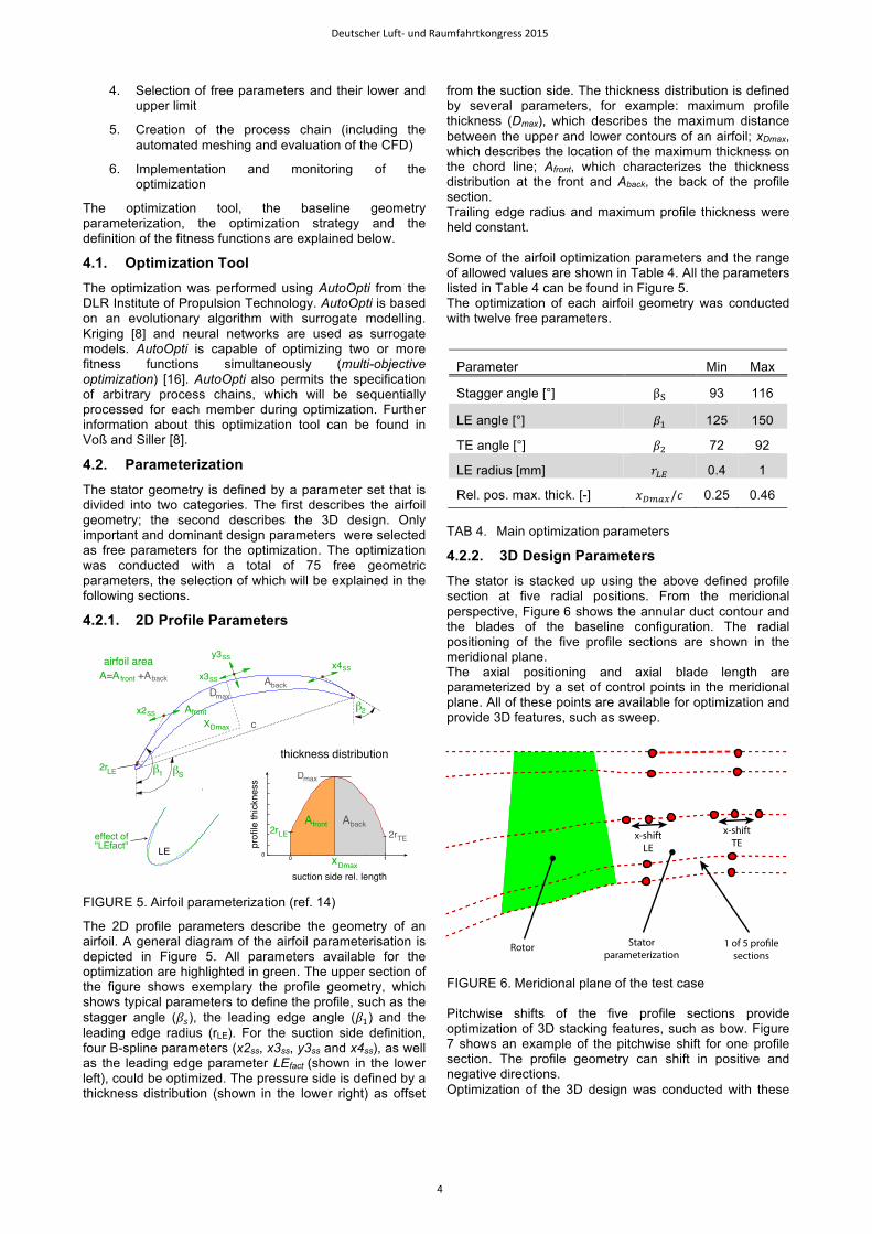
FIGURE 5. Airfoil parameterization (ref. 14)

The 2D profile parameters describe the geometry of an airfoil. A general diagram of the airfoil parameterisation is depicted in Figure 5. All parameters available for the optimization are highlighted in green. The upper section of the figure shows exemplary the profile geometry, which shows typical parameters to define the profile, such as the stagger angle (𝛽!), the leading edge angle (𝛽!) and the leading edge radius (rLE). For the suction side definition, four B-spline parameters (x2ss, x3ss, y3ss and x4ss), as well as the leading edge parameter LEfact (shown in the lower left), could be optimized. The pressure side is defined by a thickness distribution (shown in the lower right) as offset

from the suction side. The thickness distribution is defined by several parameters, for example: maximum profile thickness (Dmax), which describes the maximum distance between the upper and lower contours of an airfoil; xDmax, which describes the location of the maximum thickness on the chord line; Afront, which characterizes the thickness distribution at the front and Aback, the back of the profile section. Trailing edge radius and maximum profile thickness were held constant. Some of the airfoil optimization parameters and the range of allowed values are shown in Table 4. All the parameters listed in Table 4 can be found in Figure 5. The optimization of each airfoil geometry was conducted with twelve free parameters.

Parameter Min Max

Stagger angle [°] β! 93 116

LE angle [°] 𝛽! 125 150

TE angle [°] 𝛽! 72 92

LE radius [mm] 𝑟!" 0.4 1

Rel. pos. max. thick. [-] 𝑥!"#$/𝑐 0.25 0.46

TAB 4. Main optimization parameters

4.2.2. 3D Design Parameters The stator is stacked up using the above defined profile section at five radial positions. From the meridional perspective, Figure 6 shows the annular duct contour and the blades of the baseline configuration. The radial positioning of the five profile sections are shown in the meridional plane. The axial positioning and axial blade length are parameterized by a set of control points in the meridional plane. All of these points are available for optimization and provide 3D features, such as sweep.

FIGURE 6. Meridional plane of the test case Pitchwise shifts of the five profile sections provide optimization of 3D stacking features, such as bow. Figure 7 shows an example of the pitchwise shift for one profile section. The profile geometry can shift in positive and negative directions. Optimization of the 3D design was conducted with these

A= +A

`1 `S

`2

2rLE

x2SS

x3SS

x4SS

y3SS

thickness distribution

effect of"LEfact" LE

Aback

c

airfoil area

XDmax

ADmax

Afront back

front

Dmax

Afront2rLE 2rTE

Aback

suction side rel. length

prof

ile th

ickn

ess

10 xDmax0

Rotor 1 of 5 pro!lesections

Statorparameterization

x-shiftTE

x-shiftLE


4

parameters for each airfoil section (axial shift of leading edge, axial shift of trailing edge and circumferential shift of the profile). In summary, 12 parameters describe one blade section. In the three-dimensional space, its location is defined by 3 parameters. 5 airfoil sections build the entire blade, meaning 75 free parameters.

FIGURE 7. 3D design: pitchwise-shift

4.3. Optimization Strategy In an attempt to keep the operating range and choking mass flow constant while suppressing flow separation across the whole range, three operating points were selected for optimization:

1) Operating point 1 (OP1), working line, n = 100%

2) Operating point 2 (OP2), near surge, n = 100%

3) Operating point 3 (OP3), near surge, n = 65%

The first two operating points are depicted in Figure 4. All operating points are adjusted to a certain mass flow. The convergence criteria for the CFD simulation are the same for all members of the optimization. Fluctuation over a certain period of time was monitored for the mass-averaged efficiency, mass flow, pressure ratio and residual. The simulation was considered as converged when the fluctuation fell below 0.05%.

4.4. Fitness Function During optimization, two fitness functions are used to suppress flow separation across the whole operation range and ensure axial and homogeneous angular distribution of outflow at the ADP (OP1). One fitness function accounted for the total pressure losses (total pressure difference divided by the dynamic head at stator inlet). The total pressure loss is defined in Equation (1).

(1) 𝜔 = !!!! !!!!!!!!!"#"!

= !!!! !!!!!"#!

The other fitness function accounted for the outflow angle, as described previously.

1) Loss criterion: was defined as a weighted sum of the total pressure loss at OP1, OP2 and OP3, calculated between stator entry and exit:

(2) 𝑓! = 0.5 ∙ 𝜔!"! + 0.25 ∙ 𝜔!"! + 0.25 ∙ 𝜔!"!

2) Axial outflow criterion: was defined as an integral value of the outflow angle over the complete height of the stator at OP1:

(3) 𝑓! = (𝛽!"!"!)!! 𝑑ℎ!"#

5. OPTIMIZATION RESULTS Figure 8 shows the fitness values of all converged members of the optimization. In total 1,715 different geometries were generated during the optimization process and 761 members with converged CFD simulations are available. This kind of diagram is commonly used in multi-objective optimizations to observe the optimization process and to identify dominant members. The abscissa represents the first fitness function (Eq. 2), and the ordinate, the second fitness function (Eq. 3). As in many optimizations, the fitness functions compete. Members with high values of the first fitness function have lower values for the second fitness function and vice versa. The members with lowest values for both functions (marked with red squares) form a pareto front (marked green), which can be seen in Figure 8. In total 19 members belong to this pareto front. The fitness of the baseline geometry (the starting point of the optimization) is denoted by the pink square. The distance between the baseline geometry and the pareto front visibly demonstrates the huge potential for improvement. Therefore, improvement of the first fitness function by 30.4% and 88.1% for the second fitness function could be achieved.

FIGURE 8. Optimization database The final result of the optimization was selected of the member marked by an orange square, based on a compromise of the two fitness functions. The manufacturability of the stator geometry plays an important role, which necessitated an additional compromise between aerodynamic properties and manufacturability. The geometry shown in Figure 9 was chosen as the most promising candidate, although this solution does not have the pareto rank 1.

positivpitchwise-shift

negativpitchwise-shift

f (

)

f (Loss )

TE

0.05 0.06 0.07 0.08

0.5

1

1.5

2

baseline geometry

pareto rank 1

pareto front

1 OP1, OP2, OP3

2O

P1


5

5.1. Comparative Analysis This section presents the comparison of the aerodynamic properties and the geometry of the baseline and the optimized stator.

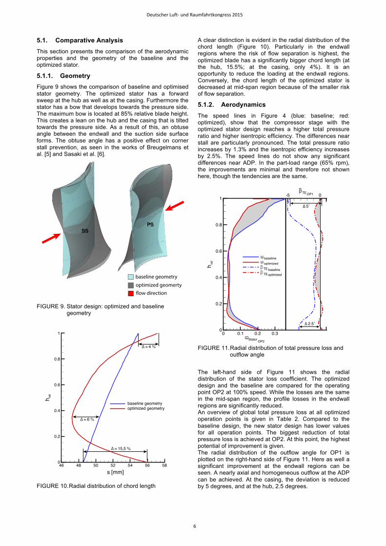
5.1.1. Geometry Figure 9 shows the comparison of baseline and optimised stator geometry. The optimized stator has a forward sweep at the hub as well as at the casing. Furthermore the stator has a bow that develops towards the pressure side. The maximum bow is located at 85% relative blade height. This creates a lean on the hub and the casing that is tilted towards the pressure side. As a result of this, an obtuse angle between the endwall and the suction side surface forms. The obtuse angle has a positive effect on corner stall prevention, as seen in the works of Breugelmans et al. [5] and Sasaki et al. [6].

FIGURE 9. Stator design: optimized and baseline

geometry

FIGURE 10. Radial distribution of chord length

A clear distinction is evident in the radial distribution of the chord length (Figure 10). Particularly in the endwall regions where the risk of flow separation is highest, the optimized blade has a significantly bigger chord length (at the hub, 15.5%; at the casing, only 4%). It is an opportunity to reduce the loading at the endwall regions. Conversely, the chord length of the optimized stator is decreased at mid-span region because of the smaller risk of flow separation.

5.1.2. Aerodynamics The speed lines in Figure 4 (blue: baseline; red: optimized), show that the compressor stage with the optimized stator design reaches a higher total pressure ratio and higher isentropic efficiency. The differences near stall are particularly pronounced. The total pressure ratio increases by 1.3% and the isentropic efficiency increases by 2.5%. The speed lines do not show any significant differences near ADP. In the part-load range (65% rpm), the improvements are minimal and therefore not shown here, though the tendencies are the same.

FIGURE 11. Radial distribution of total pressure loss and

outflow angle

The left-hand side of Figure 11 shows the radial distribution of the stator loss coefficient. The optimized design and the baseline are compared for the operating point OP2 at 100% speed. While the losses are the same in the mid-span region, the profile losses in the endwall regions are significantly reduced. An overview of global total pressure loss at all optimized operation points is given in Table 2. Compared to the baseline design, the new stator design has lower values for all operation points. The biggest reduction of total pressure loss is achieved at OP2. At this point, the highest potential of improvement is given. The radial distribution of the outflow angle for OP1 is plotted on the right-hand side of Figure 11. Here as well a significant improvement at the endwall regions can be seen. A nearly axial and homogeneous outflow at the ADP can be achieved. At the casing, the deviation is reduced by 5 degrees, and at the hub, 2.5 degrees.

baseline geometryoptimized geomerty!ow direction

s [mm]

h rel

46 48 50 52 54 56 580

0.2

0.4

0.6

0.8

1

baseline geometryoptimized geometry

¨�§ 4 %

¨�§ 15,5 %

¨�§ 6 %

Stator

TE

hrel

0 0.1 0.2 0.3

-5 0

0

0.2

0.4

0.6

0.8

1

baseline

optimized

TE baseline

TE

OP1

OP2

optimized

¨��Ý

¨��Ý


6

baseline optimized

ω!"#"$%,!"# 0.0503 0.0431 -14.31%

ω!"#"$%,!"# 0.1027 0.0593 -42.55%

ω!"#"$%,!"# 0.0654 0.0505 -22.78%

TAB 5. Total pressure loss at OP1, OP2 and OP3

Figure 12 shows the radial distribution of the de-Haller number for an operation point near stall (OP2). The de-Haller number is defined by P. De Haller [11], according to Equation (4).

(4) de-Haller = !!!!

In Equation (4), c3 defines the absolute velocity behind the stator, and c2 defines the absolute velocity in front of the stator. A stator with a global flow deceleration below 0.7 has an increased risk of flow separation. This empirical correlation applies to the baseline stator design, but in the case of the optimized 3D-design it is possible to reduce this deceleration even further. The radial distribution of flow deceleration shows that at hub and casing both stators are locally below a critical value.

The direct comparison of the optimized and baseline design reveals that the de-Haller number of the optimized stator is higher near the hub. Consequently, the hub is less loaded in the optimised stator, the load at mid-span is increased and the global flow deceleration was kept constant by the optimization. This is confirmed in numerous studies on bowed stators, for example, Weingold et al. [7]. The reason is the redistribution of blade load towards the maximum bow. The load distribution at the casing remains nearly the same.

FIGURE 12. Radial distribution of the de-Haller number at

OP2

Figure 13 shows the numerically identified streaklines along the suction side and at hub for the baseline and optimized geometry. An iso-surface that marks regions

with negative axial-velocity is also presented. Comparison of the streaklines in the baseline stator with the experiments (Figure 3) shows that the flow separation is well predicted near the shroud. Both corner stalls can be recognized in the numerical simulation but the corner stall near the hub is clearly underestimated. Comparison of the stators in Figure 13 clearly shows that the new designed stator has no signs of flow separation. The main reasons for the prevention of the corner stall are:

1. The longer chord lengths near the endwalls

2. The obtuse angle between the endwalls and the suction side surface

3. The additional radial deflection component due to the local lean at hub and shroud

Prevention of the corner stall explains the significant reduction in total pressure loss and deviation near the endwalls. In this case, the de-Haller criterion fails to predict an instable flow region near the hub and casing. Therefore, the de-Haller criterion is not suitable for predicting local flow separation for modern 3D design philosophies. The global value of 0.7 should be adapted empirically to new designs where further flow deceleration is possible.

FIGURE 13. Comparison of the streaklines along the

suction side and at hub

de-Haller

h rel

0.4 0.5 0.6 0.7 0.8 0.90

0.2

0.4

0.6

0.8

1

OP2baselineOP2optimized

baseline geometry

optimized geometry

separation line

iso-surface:neg. axial velocity


7

6. PARAMETER STUDY In this parametric study the effects of two 2D profile parameters and the bow stacking are investigated for a deeper understanding of the changes of blade shape and the resulting flow phenomena.

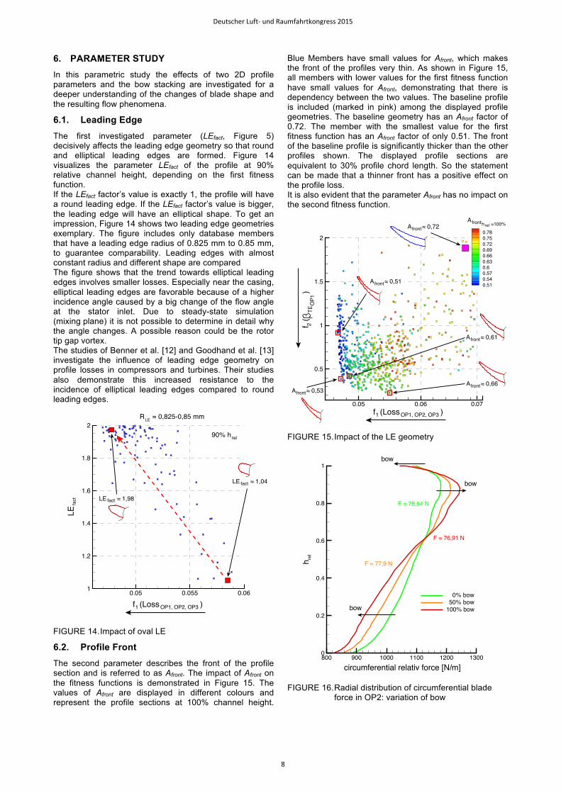
6.1. Leading Edge The first investigated parameter (LEfact, Figure 5) decisively affects the leading edge geometry so that round and elliptical leading edges are formed. Figure 14 visualizes the parameter LEfact of the profile at 90% relative channel height, depending on the first fitness function. If the LEfact factor’s value is exactly 1, the profile will have a round leading edge. If the LEfact factor’s value is bigger, the leading edge will have an elliptical shape. To get an impression, Figure 14 shows two leading edge geometries exemplary. The figure includes only database members that have a leading edge radius of 0.825 mm to 0.85 mm, to guarantee comparability. Leading edges with almost constant radius and different shape are compared The figure shows that the trend towards elliptical leading edges involves smaller losses. Especially near the casing, elliptical leading edges are favorable because of a higher incidence angle caused by a big change of the flow angle at the stator inlet. Due to steady-state simulation (mixing plane) it is not possible to determine in detail why the angle changes. A possible reason could be the rotor tip gap vortex. The studies of Benner et al. [12] and Goodhand et al. [13] investigate the influence of leading edge geometry on profile losses in compressors and turbines. Their studies also demonstrate this increased resistance to the incidence of elliptical leading edges compared to round leading edges.

FIGURE 14. Impact of oval LE

6.2. Profile Front The second parameter describes the front of the profile section and is referred to as Afront. The impact of Afront on the fitness functions is demonstrated in Figure 15. The values of Afront are displayed in different colours and represent the profile sections at 100% channel height.

Blue Members have small values for Afront, which makes the front of the profiles very thin. As shown in Figure 15, all members with lower values for the first fitness function have small values for Afront, demonstrating that there is dependency between the two values. The baseline profile is included (marked in pink) among the displayed profile geometries. The baseline geometry has an Afront factor of 0.72. The member with the smallest value for the first fitness function has an Afront factor of only 0.51. The front of the baseline profile is significantly thicker than the other profiles shown. The displayed profile sections are equivalent to 30% profile chord length. So the statement can be made that a thinner front has a positive effect on the profile loss. It is also evident that the parameter Afront has no impact on the second fitness function.

FIGURE 15. Impact of the LE geometry

FIGURE 16. Radial distribution of circumferential blade

force in OP2: variation of bow

LE

fact

0.05 0. 0.061

1.2

1.4

1.6

1.8

2

90% hrel

055

f (Loss ) 1 OP1, OP2, OP3

R = 0,825-0,85 mmLE

LE § 1,98fact

LE § 1,04fact

0.05 0.06 0.07

0.5

1

1.5

2

0.78

0.75

0.72

0.69

0.66

0.63

0.6

0.57

0.54

0.51

h =100%rel

A § 0,61front

A § 0,51front

A § 0,72front

A § 0,53front

A front

f (Loss ) 1 OP1, OP2, OP3

f (

)

T

E2

OP

1

A § 0,66front

circumferential relativ force [N/m]

h rel

800 900 1000 1100 1200 13000

0.2

0.4

0.6

0.8

1

0% bow50% bow

100% bow

F = 78,54 N

F = 76,91 N

F = 77,9 N

bow

bow

bow


8

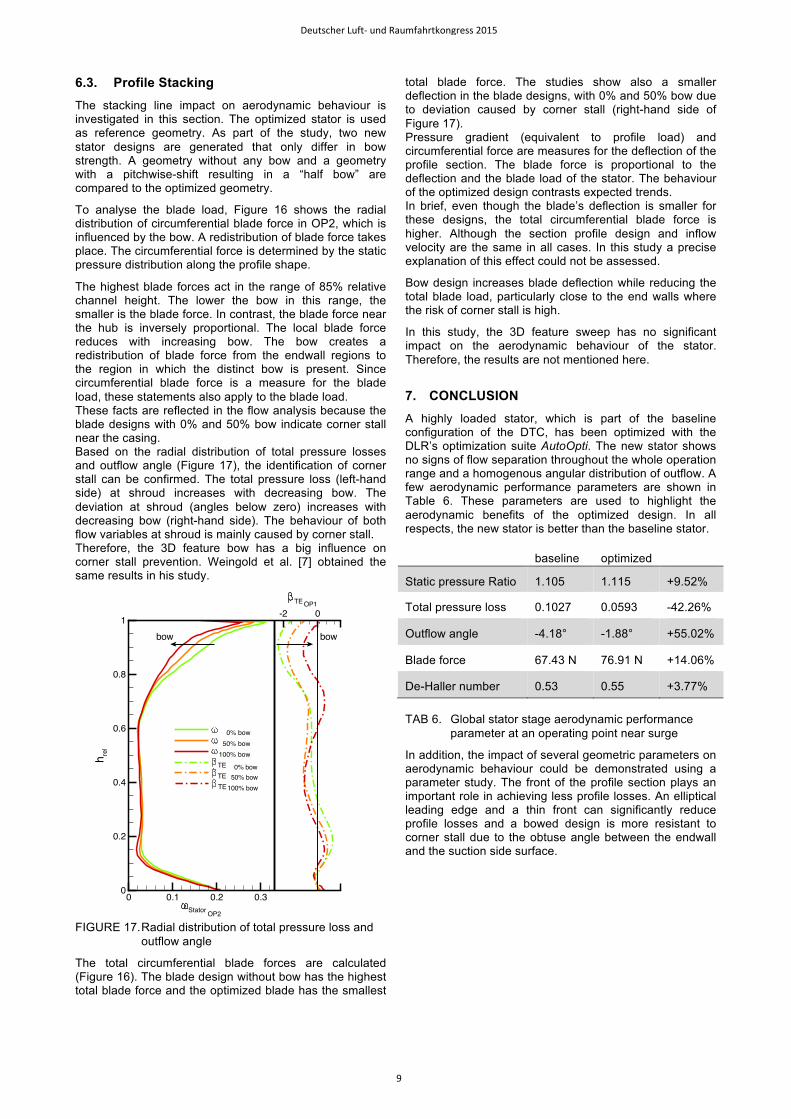
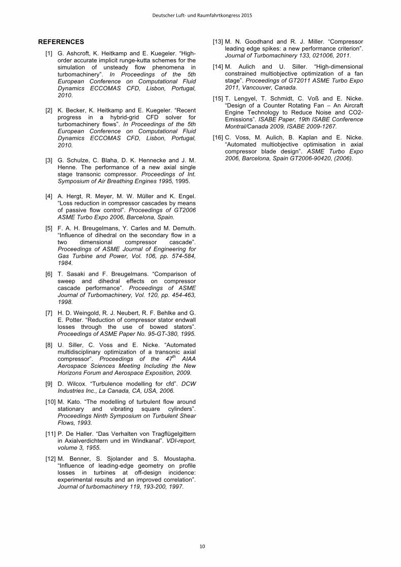
6.3. Profile Stacking The stacking line impact on aerodynamic behaviour is investigated in this section. The optimized stator is used as reference geometry. As part of the study, two new stator designs are generated that only differ in bow strength. A geometry without any bow and a geometry with a pitchwise-shift resulting in a “half bow” are compared to the optimized geometry.

To analyse the blade load, Figure 16 shows the radial distribution of circumferential blade force in OP2, which is influenced by the bow. A redistribution of blade force takes place. The circumferential force is determined by the static pressure distribution along the profile shape.

The highest blade forces act in the range of 85% relative channel height. The lower the bow in this range, the smaller is the blade force. In contrast, the blade force near the hub is inversely proportional. The local blade force reduces with increasing bow. The bow creates a redistribution of blade force from the endwall regions to the region in which the distinct bow is present. Since circumferential blade force is a measure for the blade load, these statements also apply to the blade load. These facts are reflected in the flow analysis because the blade designs with 0% and 50% bow indicate corner stall near the casing. Based on the radial distribution of total pressure losses and outflow angle (Figure 17), the identification of corner stall can be confirmed. The total pressure loss (left-hand side) at shroud increases with decreasing bow. The deviation at shroud (angles below zero) increases with decreasing bow (right-hand side). The behaviour of both flow variables at shroud is mainly caused by corner stall. Therefore, the 3D feature bow has a big influence on corner stall prevention. Weingold et al. [7] obtained the same results in his study.

FIGURE 17. Radial distribution of total pressure loss and

outflow angle

The total circumferential blade forces are calculated (Figure 16). The blade design without bow has the highest total blade force and the optimized blade has the smallest

total blade force. The studies show also a smaller deflection in the blade designs, with 0% and 50% bow due to deviation caused by corner stall (right-hand side of Figure 17). Pressure gradient (equivalent to profile load) and circumferential force are measures for the deflection of the profile section. The blade force is proportional to the deflection and the blade load of the stator. The behaviour of the optimized design contrasts expected trends. In brief, even though the blade’s deflection is smaller for these designs, the total circumferential blade force is higher. Although the section profile design and inflow velocity are the same in all cases. In this study a precise explanation of this effect could not be assessed.

Bow design increases blade deflection while reducing the total blade load, particularly close to the end walls where the risk of corner stall is high.

In this study, the 3D feature sweep has no significant impact on the aerodynamic behaviour of the stator. Therefore, the results are not mentioned here.

7. CONCLUSION A highly loaded stator, which is part of the baseline configuration of the DTC, has been optimized with the DLR’s optimization suite AutoOpti. The new stator shows no signs of flow separation throughout the whole operation range and a homogenous angular distribution of outflow. A few aerodynamic performance parameters are shown in Table 6. These parameters are used to highlight the aerodynamic benefits of the optimized design. In all respects, the new stator is better than the baseline stator.

baseline optimized

Static pressure Ratio 1.105 1.115 +9.52%

Total pressure loss 0.1027 0.0593 -42.26%

Outflow angle -4.18° -1.88° +55.02%

Blade force 67.43 N 76.91 N +14.06%

De-Haller number 0.53 0.55 +3.77%

TAB 6. Global stator stage aerodynamic performance parameter at an operating point near surge

In addition, the impact of several geometric parameters on aerodynamic behaviour could be demonstrated using a parameter study. The front of the profile section plays an important role in achieving less profile losses. An elliptical leading edge and a thin front can significantly reduce profile losses and a bowed design is more resistant to corner stall due to the obtuse angle between the endwall and the suction side surface.

hre

l

0 0.1 0.2 0.3

-2 0

0

0.2

0.4

0.6

0.8

1

StatorOP2

TEOP1

bow bow

50% bow

100% bow

TE 0% bow

TE 50% bow

0% bow

TE 100% bow


9

REFERENCES [1] G. Ashcroft, K. Heitkamp and E. Kuegeler. “High-

order accurate implicit runge-kutta schemes for the simulation of unsteady flow phenomena in turbomachinery”. In Proceedings of the 5th European Conference on Computational Fluid Dynamics ECCOMAS CFD, Lisbon, Portugal, 2010.

[2] K. Becker, K. Heitkamp and E. Kuegeler. “Recent progress in a hybrid-grid CFD solver for turbomachinery flows”. In Proceedings of the 5th European Conference on Computational Fluid Dynamics ECCOMAS CFD, Lisbon, Portugal, 2010.

[3] G. Schulze, C. Blaha, D. K. Hennecke and J. M. Henne. The performance of a new axial single stage transonic compressor. Proceedings of Int. Symposium of Air Breathing Engines 1995, 1995.

[4] A. Hergt, R. Meyer, M. W. Müller and K. Engel. “Loss reduction in compressor cascades by means of passive flow control”. Proceedings of GT2006 ASME Turbo Expo 2006, Barcelona, Spain.

[5] F. A. H. Breugelmans, Y. Carles and M. Demuth. “Influence of dihedral on the secondary flow in a two dimensional compressor cascade”. Proceedings of ASME Journal of Engineering for Gas Turbine and Power, Vol. 106, pp. 574-584, 1984.

[6] T. Sasaki and F. Breugelmans. “Comparison of sweep and dihedral effects on compressor cascade performance”. Proceedings of ASME Journal of Turbomachinery, Vol. 120, pp. 454-463, 1998.

[7] H. D. Weingold, R. J. Neubert, R. F. Behlke and G. E. Potter. “Reduction of compressor stator endwall losses through the use of bowed stators”. Proceedings of ASME Paper No. 95-GT-380, 1995.

[8] U. Siller, C. Voss and E. Nicke. “Automated multidisciplinary optimization of a transonic axial compressor”. Proceedings of the 47th AIAA Aerospace Sciences Meeting Including the New Horizons Forum and Aerospace Exposition, 2009.

[9] D. Wilcox. “Turbulence modelling for cfd”. DCW Industries Inc., La Canada, CA, USA, 2006.

[10] M. Kato. “The modelling of turbulent flow around stationary and vibrating square cylinders”. Proceedings Ninth Symposium on Turbulent Shear Flows, 1993.

[11] P. De Haller. “Das Verhalten von Tragflügelgittern in Axialverdichtern und im Windkanal”. VDI-report, volume 3, 1955.

[12] M. Benner, S. Sjolander and S. Moustapha. “Influence of leading-edge geometry on profile losses in turbines at off-design incidence: experimental results and an improved correlation”. Journal of turbomachinery 119, 193-200, 1997.

[13] M. N. Goodhand and R. J. Miller. “Compressor leading edge spikes: a new performance criterion”. Journal of Turbomachinery 133, 021006, 2011.

[14] M. Aulich and U. Siller. “High-dimensional constrained multiobjective optimization of a fan stage”. Proceedings of GT2011 ASME Turbo Expo 2011, Vancouver, Canada.

[15] T. Lengyel, T. Schmidt, C. Voß and E. Nicke. “Design of a Counter Rotating Fan – An Aircraft Engine Technology to Reduce Noise and CO2-Emissions”. ISABE Paper, 19th ISABE Conference Montral/Canada 2009, ISABE 2009-1267.

[16] C. Voss, M. Aulich, B. Kaplan and E. Nicke. “Automated multiobjective optimisation in axial compressor blade design”. ASME Turbo Expo 2006, Barcelona, Spain GT2006-90420, (2006).


10

Design and Optimization of a New Stator for the Transonic ... AND OPTIMIZATION OF A NEW STATOR FOR...

Documents

Transcript of Design and Optimization of a New Stator for the Transonic ... AND OPTIMIZATION OF A NEW STATOR FOR...