Design and Evaluation of an Improved Mixer for a

Selective Catalytic Reduction System

by

David M. Stelzer

A thesis submitted in conformity with the requirements for the Degree of Masters of Applied Science

Graduate Department of Mechanical Engineering & Industrial Engineering

University of Toronto

© Copyright by David M Stelzer (2014)

ii

Design and Evaluation of an Improved Mixer for a Selective

Catalytic Reduction System

David M Stelzer

Masters of Applied Science

Graduate Department of Mechanical Engineering & Industrial Engineering

University of Toronto

2014

Abstract

More stringent environmental regulations have created a requirement for Selective Catalytic

Reduction (SCR) after-treatment technology on stationary Diesel engines.

In this work, Computational Fluid Dynamics (CFD) is used in conjunction with a separate 1-D

catalyst reaction model to evaluate the overall performance of the combined High Efficiency

Vortab (HEV) mixer and U-bend design. This model yielded mixing results with a Uniformity

Index (UI) of 97% while generating less than 10 ppm of NH3 slip. The compact nature of the

combined design creates an SCR that is easy to install and manufacture. Pressure drop, was also

determined to be less than 10” of water (WC) over the range of operating conditions. The

performance from this design will assist engineers in meeting current and next generation

environmental regulations.

iii

Acknowledgements

The author wishes to express his sincere appreciation for all of the help and direction provided by

Professor James S. Wallace and Professor Pierre E. Sullivan toward this thesis.

The author is also grateful for the funding and support provided by the Ontario Center of

Excellence for this project and for supporting business development in Ontario. Safety Power Inc,

has also been an invaluable resource for developing this work. Special thanks to Henry Pong,

Safety Power Engineer, who has provided an incredible amount of support and assistance to this

research project.

iv

Table of Contents

1 Introduction ............................................................................................................................. 1

1.1 Selective Catalytic Reduction .......................................................................................... 1

1.2 Organization of thesis....................................................................................................... 4

2 SCR Simulations ..................................................................................................................... 5

2.1 SCR Performance Evaluation......................................................................................... 15

2.2 NOx Reduction Chemistry ................................................................................................ 5

2.3 Injection Approaches........................................................................................................ 6

2.4 Catalyst Reaction Kinetics ............................................................................................. 10

2.5 Mixing ............................................................................................................................ 11

3 Numerical Set-Up ................................................................................................................. 17

3.1 U-bend SCR Design ....................................................................................................... 17

3.2 Geometry ........................................................................................................................ 18

3.3 Flow Regime .................................................................................................................. 21

3.4 Meshing .......................................................................................................................... 23

3.5 Injection .......................................................................................................................... 26

3.6 Dimensional Catalytic Reaction Model ......................................................................... 31

3.7 Numerical Error.............................................................................................................. 35

4 Results and Discussion ......................................................................................................... 45

4.1 HEV Model .................................................................................................................... 45

4.2 HEV and U-bend Performance ...................................................................................... 49

4.3 NOx and NH3 Results from UWS Simulation ................................................................ 53

5 Conclusions and Recommendations ..................................................................................... 62

5.1 Future Recommendations ............................................................................................... 63

6 References: ............................................................................................................................ 65

v

List of Figures

Figure 1-1: US EPA Off Road Emissions Regulations (Xinqun et al. 2010) ................................. 3

Figure 2-1: HEV Based Static Mixer ............................................................................................ 14 Figure 3-1: Overall SCR Geometry .............................................................................................. 18 Figure 3-2: Upstream DPF Box .................................................................................................... 19 Figure 3-3: Side View of the Complete Mesh .............................................................................. 23 Figure 3-4: Horizontal Mid-Plane Contour Plot of Y+ Values .................................................... 25

Figure 3-5: Urea Decomposition with UWS Model (Birkhold et al. 2007) ................................ 28 Figure 3-6: Overall SCR Modeling (Faltsi & Mutyal 2012). ....................................................... 31

Figure 3-7: Geometric Configuration of SCR Only Design ......................................................... 37 Figure 3-8: Extrapolated Value of Axial Velocity across Catalyst Face ...................................... 39

Figure 3-9: Extrapolated Value of NH3 Concentration across Catalyst Face ............................... 40 Figure 3-10: Extrapolated Value of Static Pressure across Catalyst Face .................................... 40

Figure 3-11: GCIfine with Error Bars of Axial Velocity across Catalyst Face .............................. 42 Figure 3-12: GCIfine with Error Bars of NH3 Concentration across Catalyst Face ....................... 42 Figure 3-13: GCIfine with Error Bars of Static Pressure across Catalyst Face ............................ 43

Figure 3-14: Residual Plot for Fine Mesh with Injection ............................................................. 44 Figure 4-1: HEV Only Mixer ........................................................................................................ 46

Figure 4-3: HEV Mixer Full Load Performance........................................................................... 47 Figure 4-4: Mid-Plane Total Pressure Contour Plot of HEV Only Mixer .................................... 48

Figure 4-5: HEV Mixer, Water Spray Partial Loading Performance ........................................... 49 Figure 4-6: Pathlines for Full Load U-Bend Model ...................................................................... 50

Figure 4-7: Pathlines for Full Load Combined HEV and U-Bend Model .................................... 50 Figure 4-8: U-bend Only Model, Molar Feed Ratio across Catalyst ............................................ 51 Figure 4-9: Combined HEV and U-bend Model, Molar Feed Ratio across Catalyst ................... 52

Figure 4-10: Mid-Plane Contour Plot of Axial Velocity .............................................................. 54 Figure 4-11: Mid-Plane Contour of Total Pressure ...................................................................... 55

Figure 4-12: Mid-Plane Contour Plot of Temperature ................................................................. 56 Figure 4-13: Mid-Plane Contour of Full Load HNCO Concentrations ........................................ 57 Figure 4-14: Mid-Plane Contour of Full Load NH3 Concentrations ............................................ 57 Figure 4-15: Normalized Axial Flow Velocity Across Catalyst Face .......................................... 58 Figure 4-16: Normalized HNCO Concentration Across Catalyst Face ........................................ 59

Figure 4-17: Normalized NH3 Concentration Across Catalyst Face ............................................ 59

vi

Nomenclature

Latin letters

A pre-exponential factor (1/s)

Ag cross-sectional area of catalyst wall (μm)

Ai cell area (m2)

Ap surface area of droplet (m2)

Aw cross sectional area of void channel (μm)

𝐶𝑖,∞ vapour concentration in bulk gas (kmol/m3)

Ci,s vapour concentration at droplet surface (kmol/m3)

cp specific heat (J/kg-K)

Cp,g specific heat of gas (J/kg-K)

Cp,w specific heat of gas at wall (J/kg-K)

d droplet diameter (μm)

dh hydraulic diameter (m)

dm mean droplet diameter (μm)

Dm mass diffusion coefficient (m2/s)

𝑒𝑖 unit vector

Ea activation energy (kJ/mol)

Ea d activation energy of desorption reaction (kJ/mol)

Ea o activation energy of oxidation reaction (kJ/mol)

Ea r activation energy of reduction reaction (kJ/mol)

h non-dimensionalized mesh size

hc convective heat transfer coefficient (W/m2-K)

hf g latent heat of vaporization (kJ/kg)

𝑘∞ thermal conductivity of continuous phase (W/m-K)

kc mass transfer coefficient(m/s)

L catalyst length (m)

md mass of droplet (kg)

ṁvap mass flow of vaporization (kg/s)

n spread parameter

N number of cell elements

P pressure (Pa)

pa pre-exponential factor for absorption (1/s)

pd pre-exponential factor for desorption (1/s)

vii

po pre-exponential factor for oxidation (1/s)

pstat saturated vapour pressure (Pa)

R Universal gas constant (J/mol-K)

ri j ratio of h values, (hj/hi)

s storage sites per meter (m-1)

Δt time step (s)

t time (s)

𝑇∞ temperature of bulk gas (K)

Tg temperature of gas (K)

Tp temperature of particle (K)

Tw temperature of gas at wall (K)

udarcy Darcy friction factor

U x component of velocity (m/s)

V y component of velocity (m/s)

ΔVi element volume (m3)

�� cell velocity vector (m/s)

�� Velocity field (m/s)

W z component of velocity (m/s)

Y+ non-dimensional distance from wall

Yd mass fraction of droplet greater than d

𝑌𝑖,∞ vapour mass fraction in bulk gas

Yi,s vapour mass fraction at surface

Yu Mass fraction of urea

Greek letters

∇ del operator

Øi cell field property

α molar feed ratio

εp particle emissivity

θ fraction of ammonia storage

θR radiation temperature, (I/4σ)1/4, where I is the radiation intensity

μ molecular viscosity (kg /s2)

𝜌∞ density in bulk gas (kg/m3)

ρg density in gas (kg/m3)

ρw density in gas at wall (kg/m3)

σ Stefan Boltzmann constant (5.67 x 10-8 W/m2-K4)

viii

Dimensionless numbers

Pr Prandtl number, (cp∙μ/𝑘∞)

Re Reynolds number, (ρg∙dh∙U/μ)

Sc Schmidt number, (μ/ρg-Dm)

Sh Sherwood number, (kc∙L/Dm)

1

1 Introduction

1.1 Selective Catalytic Reduction

NOx emissions are one of the key contributors to the formation of smog and greenhouse

gases. This has been related to several adverse health conditions, global warming, acid rain and is

the reason for new environment regulations.

NOx emissions are comprised of two gases that can form in high temperature combustion process;

these two gases are Nitric Oxide (NO) and Nitrogen Dioxide (NO2). In most current engine

applications, NOx is created by the high temperature level achieved in the combustion chamber.

The chemical reactions that form the gases at high temperatures (the thermal mechanism for NOx

formation) are (Heywood 2011):

(1-1)

𝑂 + 𝑁2 → 𝑁𝑂 + 𝑁

(1-2)

𝑁 + 𝑂2 → 𝑁𝑂 + 𝑂

(1-3)

𝑁 + 𝑂𝐻 → 𝑁𝑂 + 𝐻

(1-4)

𝑁𝑂 + 𝐻𝑂2 → 𝑁𝑂2 + 𝑂𝐻

(1-5)

𝑁𝑂2 + 𝑂 → 𝑁𝑂 + 𝑂2

2

In the past, NOx emissions have been controlled within the combustion process; some examples

for diesel engines include:

High Pressure Direct Injection, with multiple injections during combustion cycle reducing

peak pressure and temperature (Fang et al. 2008).

Exhaust Gas Recirculation (EGR), recycled gas reduces peak combustion temperatures by

increasing the heat capacity of intake gases.

Engine intercoolers or aftercoolers, reduce the temperature of turbocharged intake air

(Heywood 2011).

Current regulations are too stringent to achieve with combustion process control alone. Some form

of exhaust after-treatment is required. At temperatures between 1,200K and 1,300K NOx can be

reduced into Nitrogen Gas by injecting ammonia into the exhaust stream, this is referred to as the

Selective Non-Catalytic Reduction (SNCR) process (Zamansky et al. 1999).

Reduction can be carried out at the lower temperatures typical of engine exhaust through the use

of a catalyst in a process known as Selective Catalytic Reduction (SCR). Lower temperature SCR

after-treatment technologies were first employed to reduce NOx in industrial power plants in the

1980s (Depcik & Assanis 2005). Since then, the technology has been extended to the automotive

industry where it was first introduced in the Mercedes G-Class Bluetech vehicle (Chatterjee et al.

2008). In automotive and stationary engine technologies, ammonia is provided in the form of urea-

water solution, a liquid that is easy to store and handle.

SCR technology has several advantages in delivering a high degree of NOx reduction:

Durability

No additional burner or oxidation catalyst required

3

No additional fuel input

Low Pressure Drop

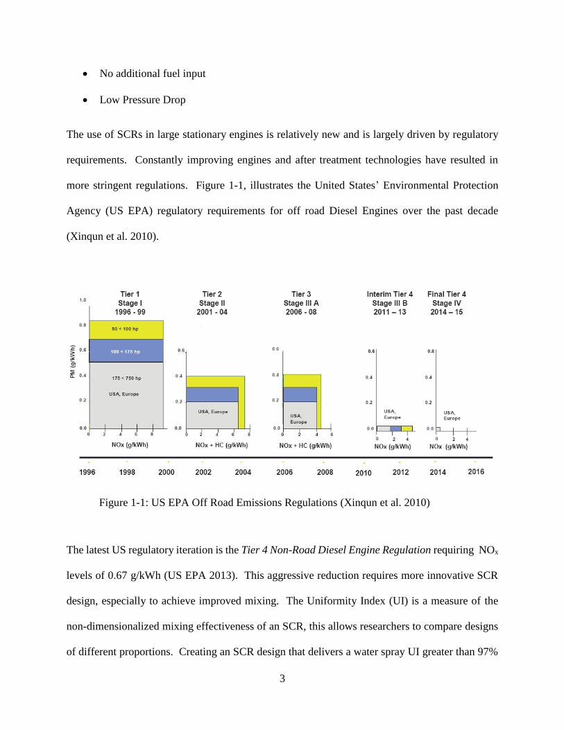
The use of SCRs in large stationary engines is relatively new and is largely driven by regulatory

requirements. Constantly improving engines and after treatment technologies have resulted in

more stringent regulations. Figure 1-1, illustrates the United States’ Environmental Protection

Agency (US EPA) regulatory requirements for off road Diesel Engines over the past decade

(Xinqun et al. 2010).

Figure 1-1: US EPA Off Road Emissions Regulations (Xinqun et al. 2010)

The latest US regulatory iteration is the Tier 4 Non-Road Diesel Engine Regulation requiring NOx

levels of 0.67 g/kWh (US EPA 2013). This aggressive reduction requires more innovative SCR

design, especially to achieve improved mixing. The Uniformity Index (UI) is a measure of the

non-dimensionalized mixing effectiveness of an SCR, this allows researchers to compare designs

of different proportions. Creating an SCR design that delivers a water spray UI greater than 97%

4

would surpass current designs (Pong 2010). Relating the UI to the Tier 4 regulation, involves

combining the UI with specific engine characteristics and catalyst reaction kinetics.

SCR technology has become a widely accepted approach for reducing NOx emissions associated

with large stationary engines. Computational Fluid Dynamics (CFD) is increasingly used to

optimize SCR design through modelling. Modelling an SCR requires describing injection, mixing

and the reaction kinetics important to reducing NOx. The goal of this thesis is to create a novel

mixing design that improves SCR performance for large stationary engines.

1.2 Organization of thesis

Enhancing SCR mixing using CFD modeling is the goal of this thesis. This thesis will first focus

on understanding the NOx reduction process and the current approaches for achieving this. A

description of the geometric design and modelling approach will then be outlined. A specific

design will then be evaluated using this model and analyzed to show an increase in performance.

5

2 SCR Simulations

This chapter summarizes the phenomena underlying operation of an SCR system, including NOx

reduction chemistry, urea injection approaches, catalyst reaction kinetics and mixing. Finally, two

criteria for SCR performance valuation are presented.

2.1 NOx Reduction Chemistry

The SCR catalyst is referred to as “selective” as it only absorbs NH3 resulting in reduced NOx

emissions from the exhaust. Non-selective Oxidation catalysts are often used in conjunction with

an SCR to remove excess hydrocarbons (King 2007). There are six reactions that can occur when

NOx comes into contact with ammonia over a selective catalyst:

(2-1)

4NH3 + 2NO + 2NO2 -> 4N2 + 6H2O

(2-2)

2NH3 + NO + NO2 -> 2N2 + 3H2O

(2-3)

8NH3 + 6NO2 -> 7N2 + 12H2O

(2-4)

4NH3 + 3O2 -> 2N2 + 6H2O

(2-5)

2NO + O2 <-> 2NO2

(2-6)

2NH3 + 2NO N2 + N2O + 3H2O

6

Equations (2-1) and (2-4) are the most prevalent in the SCR process; they are respectively referred

to as the ammonia reduction and oxidation reactions. The remaining equations have slow rates of

reaction and are neglected in modelling(Faltsi & Mutyal 2012).

2.2 Injection Approaches

Initially, industrial based SCRs used pure ammonia gas for injection. To reduce the risks

associated with storing liquid ammonia, a low concentration urea solution is now used for

commercial applications. A standard urea solution containing 32.5% by weight of ammonia

solution in water is used for these applications. Urea water solutions are easy to transport as they

are non-volatile (King 2007).

For the urea to be useful in the SCR, it must be converted into ammonia gas and this process occurs

in three steps. First, water is vaporized from the droplet and evaporates from water-urea droplets

at 373 K at 1 atm. Continued water evaporation increases the urea concentration of the droplet

until saturation occurs. A thin layer of urea salt is then created; further saturation forms a hollow

sphere urea particle structure (Kulmala & Wagner, 1996). Equation (2-7) models the water

evaporation from urea which occurs before the exhaust flow encounters the catalyst. The second

step, takes place when the remaining solid urea melts at 425 K at 1 bar and decomposes to form

isocyanic acid (HNCO) and ammonia gas. The production of isocyanic acid and ammonia

(Equation ((2-8)) occurs quickly before the exhaust stream contacts the catalyst (Birkhold et al.

2006). The last step, is the decomposition of isocyanic acid into ammonia gas and carbon dioxide.

The corresponding chemical formula is shown in Equation (2-9). This reaction typically takes

place on the catalyst surface. Summating the entire process yields 2 moles of gaseous ammonia

per mole of solid urea (Ström et al. 2009).

7

(2-7)

(NH2)2CO (aq) (NH2)2CO(s or l) + 6.9H2O(g)

(2-8)

(NH2)2CO(s or l) NH3(g) + HNCO(g)

(2-9)

HNCO(g) + H2O(g) NH3(g) + CO2(g)

Research has focused on modeling the urea water decomposition process using CFD (Birkhold et

al. 2006; Wang et al. 2009; Kim et al. 2004). The simplest way to simulate this process is the

Water Spray Model, which treats the urea as water droplets. This model over-predicts urea

decomposition, at it assumes that all evaporated water will be immediately converted into

ammonia. In practice, decomposition occurs quickly, but not until the urea particle reaches 425K

at 1 atm. This model also does not distinguish between ammonia and isocyanic acid and assumes

that the urea decomposition occurs in one step (Helden et al. 2004). Generally catalysts are

designed with larger axial distances allowing the isocyanic acid to decompose. Since most

isocyanic acid decomposes on the catalyst surface, ignoring the proceeding rate of reaction is a

fairly good approximation. The advantage of using a Water Spray model is a large reduction in

computational expense as no reaction kinetics are required. The Water Spray approach has been

used to accurately evaluate SCR design using CFD (Helden et al. 2004)

More inclusive Urea decomposition models account for both the urea and water constituents and

are referred to as Urea Water Solutions (UWS). There are two prevalent models that have been

used for describing this decomposition process. The first is the Wet-Solid Combustion Model

which evaluates the UWS particle as solid urea and liquid water. This model is well established in

8

modeling reactions in combustion chambers and uses diffusion and convection to model the

evaporation of the water from the UWS particle. At the same time, a single rate based equation is

employed to describe the melting of urea into ammonia. The wet-solid approach to model urea

decomposition is employed in this thesis and is described in detail in Section 3.5. Experimentation

using a long tube with several longitudinal samplings ports was used to verify that this model

yields accurate results (Kim et al. 2004).

A Multi-Component UWS Model has also been utilized to describe urea decomposition. This

model treats the UWS droplet as a homogenous liquid urea and water particle. Diffusion and

convection or rapid mixing are used to describe the vaporization of the entire particle solution.

Thermolysis of the solution is described using Raoult’s Law and Dalton’s Law for partial and total

vapour pressures (Birkhold et al. 2006).

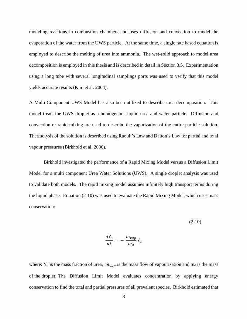
Birkhold investigated the performance of a Rapid Mixing Model versus a Diffusion Limit

Model for a multi component Urea Water Solutions (UWS). A single droplet analysis was used

to validate both models. The rapid mixing model assumes infinitely high transport terms during

the liquid phase. Equation (2-10) was used to evaluate the Rapid Mixing Model, which uses mass

conservation:

(2-10)

𝑑𝑌𝑢

𝑑𝑡= −

��𝑣𝑎𝑝

𝑚𝑑𝑌𝑢

where: Yu is the mass fraction of urea, ��𝑣𝑎𝑝 is the mass flow of vapourization and md is the mass

of the droplet. The Diffusion Limit Model evaluates concentration by applying energy

conservation to find the total and partial pressures of all prevalent species. Birkhold estimated that

9

both models yield similar results. The one exception, is that the Diffusion Limit model predicts a

slightly higher urea concentration at the catalyst face; he concluded that this small increase in

performance is not worth the extra computational power required. Birkhold estimates that the

Diffusion Limit Model is 10 times more computationally expensive. Both of these models were

compared to experimental results and were determined to align accurately (Birkhold et al. 2007).

Droplet size can also affect the decomposition process. Experiments have determined that

particles less than 150 µm in diameter behave as described by the 3 part decomposition process,

presented earlier in this Section. Larger particles break down differently and have been shown to

form a protective surface skin when heated. This protective skin inhibits the regular evaporation

and eventually causing the droplet to explode when sufficient heat has been supplied. This

protective skin requires more energy to decompose and results in a longer evaporation period

(Vahid 2011).

Air assisted injectors are commonly used for urea injection for Stationary Engine SCRs. These

injectors combine compressed air with liquid urea to atomize the solution. An upstream urea pump

works in conjunction to deliver the correct quantity of solution. Air assisted injectors produce

small droplets (mean diameter of 30 µm) when compared to automotive airless injection systems.

Small droplets are advantageous as they evaporate quickly allowing a reduction in the SCR mixing

length (Helden et al. 2004). Similar SCR designs utilizing these injectors have also not exhibited

any flashed urea within the injector (Safety Power Inc 2013).

Droplets from air assisted injectors have been shown to behave in accordance with a Rosin

Rammler statistical distribution. This statistical model has been widely used to predict the size of

10

urea droplets injected into a SCR as it accurately models droplet formation. The Rosin-Rammler

model is (Jeong et al. 2008):

(2-11)

𝑌𝑑 = 𝑒𝑥𝑝 [−(𝑑

𝑑𝑚)𝑛

]

where: Yd is the mass fraction of the droplet greater the d, d is the droplet diameter, dm is the mean

droplet diameter and n is the spread parameter.

2.3 Catalyst Reaction Kinetics

Understanding the reaction kinetics within the catalyst is essential for determining the

corresponding effectiveness and also vital for creating control strategies in commercial designs.

Catalyst based reaction models were initially developed for 3 way automotive catalysts in the early

1970s. These models have been accurately applied to evaluate SCR catalyst performance (Depcik

& Assanis 2005). Initial models neglected catalyst ammonia storage terms, limiting them to steady

state situations.

The requirement for better SCR control has focused on the effects of modulating the amount of

injectant compared to NOx in the exhaust stream. Too much injectant leads to excellent NOx

reduction, but creates NH3 slip and it has been found that the ideal injection rates are slightly less

than stoichiometric (Helden et al. 2004). Transient SCR injection models are much more complex

as the catalyst is able to store ammonia. To evaluate a suitable model, Hsieh set up an experimental

reactor with NH3 sensors positioned before, after and at the midpoint of the catalyst. He compared

the experimental results to a 1D Continuously Stirred Tank Reactor (CSTR) model and found that

11

the results agreed well (Hsieh & Wang 2011). External 1-dimenional models can be used to predict

final NOx and NH3 slip concentrations (Depcik & Assanis 2005). This thesis utilizes this

(described in Section 3.6). Recent literature has focused on solving models of these transient

catalysts quickly so that they can be adopted into real time control systems. Linearized 1-D models

with catalyst storage terms have shown particularly good computational performance for solving

these control problems (Na 2010).

2.4 Mixing

Straight mixing chambers with few mixing features were used in early commercial SCRs to satisfy

the initial regulations of NOx conversion rates of approximately 50%. Since then, SCR designs

have become much more innovative to meet increasing requirements (King 2007). Understanding

mixing geometry and the addition of mixing features to improve NOx conversion is essential to

produce a competitive SCR product.

Flow in the mixing portion of the SCR is highly turbulent with Reynolds numbers ranging from

50,000 to 250,000. Mixing can be enhanced by angling the injector or modifying the flow around

the injector. Ström et al. (2009) performed his analysis on a straight reactor with an injecting lance

mounted at 45o. This design was evaluated using CFD and variable duct lengths. The longest duct

length yielded the best results with a 65% conversion rate. Helden et al. (2004), created a custom

injector lance with 8 ports. The injection lance was mounted parallel to the flow so that the injector

ports sprayed at acute angles towards the flow. This design was also combined with a 90o

geometric bend after the injection. The combination of these two mixing features yielded

conversion rates over 90% (Helden et al. 2004).

12

Pong et al. (2012) used a 3D Fluent model to evaluate the performance of a U-bend design.

The U-bend creates a 180o bend between the injector location and the catalyst inlet. This design

worked extremely well, as it created a recirculation zone on the far side of the U-bend. This

recirculation zone resulted in a pressure gradient that bent the flow evenly onto the surface of the

catalyst. Three variants of the design were created by modifying the cross sectional ratio of height

to width. The best performing cross sectional design involved a slightly higher height to width

ratio of 1.25. At high engine loads this design yielded UI values of 95% with minimal amounts of

NH3 slip. Pong also experimentally verified his results and did not observe any appreciable wall

wetting (Pong et al. 2012).

Geometric features can also be used to enhance the dispersion of the injectant in the reactor.

Oh et al. (2012), used mixing plates to enhance the mixing in a Lean NOx trap. A Lean NOx trap

is another type of NOx after-treatment system. The NOx trap contains a catalyst that has the ability

to store NOx during lean combustion conditions and release the accumulated NOx during rich fuel

conditions. NOx released in high concentrations will have a high NO2 conversion rate. This

experiment utilized a fuel injector before the lean NOx trap to create rich conditions for a direct

injection gasoline engine. The injector dynamics described above have similar flow characteristics

to an SCR; the mixer behavior can therefore be utilized to improve SCR performance. This

experiment used high speed photography to evaluate the performance of the mixing plates that

were placed downstream of the injector. Two types of mixing plates were investigated, a grid-

plate mixer and a vortex mixer with a helical contour. The vortex mixer, actually reduced

performance of the lean NOx trap as it created a destabilization of the flow and resulted in wall

wetting. It was theorized that this destabilisation was likely the result of the helical design and the

13

placement of the injector. The grid-plate mixer enhanced the UI index by 15-20% over a range of

engine loading conditions (Oh et al. 2012).

To push the boundaries of SCR design, different processes with similar type mixing

conditions were researched to see if other relevant mixing enhancements or technologies could be

introduced. Commercial natural gas turbines used in power generation were of interest. NOx

concentrations are also a concern in modern day power generation turbines. One way of reducing

NOx is to employ a lean-premix strategy in the combustor. Much like an SCR, fuel is injected

through a lance into the combustor portion of the turbine; uniform mixing in 1.5 diameters is

required for this process. Eroglu et al. (2001) used Laser Doppler Anemometry and Laser Induced

Florescence to optically evaluate the performance of up-stream delta wing vortex generators in gas

turbines. This experiment used similar types of flows (Re = 50,000) and experimentally simulated

the flow using a water channel experimentation apparatus. In this apparatus a constant flow of die

injected water is passed over the plates and evaluated using the optical devices mentioned above.

The images obtained were then examined using commercial imaging and statistical software

packages. Pressure drop was also calculated by determining the vorticity and circulation of the

flow using Equations (2-12) and (2-13).

(2-12)

�� = ∇ × �� = (𝜕

𝜕𝑥𝑒 𝑥 +

𝜕

𝜕𝑦𝑒 𝑦 +

𝜕

𝜕𝑧𝑒 𝑧) × (𝑈𝑒 𝑥 + 𝑉𝑒 𝑦 + 𝑊𝑒 𝑧)

(2-13)

ℶ = ∬ �� ∙ 𝑑𝑆

𝒔

14

where: 𝑒 𝑥, 𝑒 𝑦 𝑎𝑛𝑑 𝑒 𝑧 are Cartesian unit vectors and U, V and W are the corresponding velocity

components. It was determined that delta wing generators with a cross section of 50% more length

than width yielded the best results with little recirculation. This configuration of delta wing yielded

uniform mixing at 3 diameters with a 5% pressure drop. In order to obtain uniform mixing in the

required 1.5 diameters, 4 parallel delta wing generators were combined. Combining the delta

wings increased the pressure drop to 30%. Another interesting observation is that the resulting

flows did not have any flow impingement after the delta wing vortex generators, which is

analogous to no wall wetting in an SCR design (Eroglu et al. 2001).

Another interesting mixer design was found investigating static mixers used in industrial process

based applications. In particular, the High Efficiency Vortab (HEV) mixer developed by Vortab

Corporation is used in similar flow regimes to enhance mixing (Smith 1990). Figure 2-1, illustrates

the geometry of a HEV mixer

Figure 2-1: HEV Based Static Mixer

15

The HEV mixer contains 2 circular mixer areas that each have several angled vanes. The vanes

contained within each circular mixer area are all the same size and at the same angle with respect

to the axial length. The HEV mixer has been previously modeled in CFD and has shown excellent

turbulent liquid to gas mixing. A HEV mixer was one of the mixing components utilized in this

thesis as it has shown excellent mixing with relatively little pressure drop or swirl. (Bakker &

Laroche 2000).

2.5 SCR Performance Evaluation

The two most critical SCR design variables that evaluate overall performance are NOx reduction

and NH3 slip. NH3 slip occurs when excess ammonia is emitted to atmosphere. Regulations

generally dictate a maximum allowable ammonia slip of 10ppm for SCR design Ammonia is

dangerous as it toxic. It is also extremely volatile and will combine to form harmful substances

like ammonium sulfate and ammonium nitrate salts (King 2007). Designing an SCR that does not

meet ammonia slip requirements would be unsafe; therefore minimizing NH3 slip is a fixed design

criteria.

NOx reduction depends on how effectively ammonia mixes with exhaust gas. Large NOx reduction

or conversion is the goal of any SCR design. A high degree of uniformity at the entrance of the

catalyst also results in longer catalyst life and reduces the amount of the catalyst required for

overall NOx conversion. The UI is an effective way of evaluating the mixing process as is can be

used to non-dimensionally compare different SCR designs (Oh et al. 2012). The UI is calculated

at the inlet of the catalyst portion of the SCR using Equation (2-14).

16

(2-14)

𝑈𝐼 = 1 −∑ [(|∅𝑖 − ∅𝑚|)(|𝐴𝑖|)]

𝑛𝑖=1

2|∅𝑚| ∑ [|𝐴𝑖|]𝑛𝑖=1

where: Øi is the property of interest, Øm is the mean value of that properties and Ai is the cell area.

The following specific performance criteria have been selected for the enhanced mixing SCR

design:

Able to reduce NOx emission by creating pre-catalyst mixing water spray concentration

with a UI greater than 97% for particular loading conditions.

Achieve this NOx reduction while maintaining concentrations of less than 10 PPM of

ammonia slip in the treated exhaust stream.

Achieve these performance characteristics with a pressure drop less than 10” of water.

Use a single urea injector to achieve the results.

Minimize axial mixing lengths so that the design is compact and easy to apply in retrofit

applications.

17

3 Numerical Model

This chapter presents the U-bend SCR design, geometry and the mesh used in the simulation. The

flow regime in the SCR is calculated for three engine loads. Input data for urea injection and the

one-dimensional catalyst model are summarized and discussed. Finally, the results of a

comprehensive error analysis are presented to demonstrate the adequacy of the mesh used in the

simulations.

3.1 U-bend SCR Design

The SCR design studied in this thesis uses a U-bend for improved flow uniformity across the

catalyst face. The 180o bend performs this by creating a recirculation zone in the middle of the

bend, guiding the flow around it and generating mixing. A U-bend type design has been shown to

deliver UI values over 95% (Pong et al. 2012) with low pressure loss, pressure loss is a major

concern to large scale commercial Diesel engines. Market dominant inline SCRs require mixing

lengths similar to that of a U-bend design, creating an overall mixer requiring twice the axial

length. The compact design of the U-bend reduces production costs and enables SCRs to easily be

retrofitted to existing space-constrained stationary Diesel engines (Pong et al. 2012).

To achieve a higher degree of mixing, an HEV based static mixer was added to a U-bend design

to enhance upstream mixing and overall performance. A multiple injector design was also

considered, but limited availability of commercial urea injectors with flow rates less than 1 kg/hour

(Spraying Systems Co, 2013) constrained the commercialization of this type of design. Multiple

injector designs also create complicated control strategies as there is an increase in the number of

control points. For these reasons the addition of an upstream HEV mixer was researched as a way

to achieve a Tier 4 level of performance.

18

3.2 Geometry

The geometry consists of three main parts:

An upstream Diesel Particulate Filter (DPF). While not the focus of this thesis, it is

important to understand the behaviour as the DPF outlet area establishes the SCR inlet

boundary conditions

A mixing duct, which is a combination of a tubular HEV mixer and a square duct U-bend.

The Urea injector is also located near the front of this assembly.

A catalyst section, which consists of a Vanadium Titania (V2O5-WO3/TiO2) based

monolithic porous catalyst.

The final geometry is shown in Figure 3.1.

Figure 3-1: Overall SCR Geometry

19

The green rectangular section in Figure 3.1 represents an exhaust inlet for the SCR. There are two

identical inlets, the second one is not shown in Figure 3.1, but is identical except that it is mirrored

across the Z-axis. The outlet is represented by the green circle on top of the SCR.

The complete upstream DFP is not shown in Figure 3.1. A DPF would be placed over the area

combining the inlets with the hollow rectangular area, or DPF pressure box. The DPF works by

distributing the pressurized flow through several small porous channels, removing particulate

matter from exhaust gas. A pressure drop of 2” to 6” of water column has been observed with

similar stationary DPFs (Mansour 2005); however, it seemed to result in uniform velocity

distribution across the SCR system inlet boundaries. The porous channels contained within the

DPF, are typically 20-30 cm in length, resulting in an exit flow normal to the SCR system inlets.

Figure 3-2 shows the geometry of the DPF box.

Figure 3-2: Upstream DPF Box

20

Exhaust gas enters the SCR system inlet faces shown in Figure 3.1 and is then directed towards

the tubular opening of the HEV mixer. At the front of the mixer is an aqueous urea injector.

Downstream of the mixer there is an expansion zone followed by the U-bend that turns the flow

180o before reaching the catalyst face. After the flow has passed through the catalyst zone, there

is a collection area and vertical outlet stack. The exhaust outlet vents to atmosphere and the outlet

was assumed to have a uniform normal flow distribution.

Engine emission characteristics for a Cummins QSK50-54 were used and are shown in Table 3.1

below (Cummins 2013):

Engine Load (%) Exhaust Flow Rate (kg/h) Exhaust Temperature (K)

10 3,813 600

45 6,162 650

100 9,854 700

Table 3-1: Engine Exhaust Flow Rates and Temperature

The chemical composition of exhaust entering the SCR was modeled with: 74% N2, 10% O2, 9%

CO2 and 7% H2O by volume. The SCR inlet composition was kept constant for all engine loading

conditions shown in Table 3.1, as varying load performance was not published by Cummins. All

flow in the SCR was assumed to be incompressible.

Flow through the catalyst section was modeled as flow through a porous media. The small cross

sectional size of the catalyst channels causes the flow to behave in the laminar regime with a

Reynolds Number around 1000. Convection, acceleration and diffusion can all be neglected in the

catalyst, allowing Darcy`s Law to be utilized. Darcy’s Law (Equation (3-1) is used to determine

the resistance coefficients (1/α) for the catalyst.

21

(3-1)

∆𝑃

𝐿=

1

𝛼𝜇|𝑢𝑑𝑎𝑟𝑐𝑦|

where: P is pressure, L is the axial catalyst length, α is the molar feed ratio, μ is the molecular

viscosity and udarcy is the Darcy friction factor.

3.3 Flow Regime

ANSYS Fluent V14.5 was used to model the SCR design, as it is widely used (Kuehlert et al.

2008)(Jiang et al. 2011)(Gröhn et al. 2012). A k-ϵ RANS model was selected as the flow is highly

turbulent; the Reynolds Numbers corresponding to the range of engine loads simulated are shown

in Table 3-2. The k-ϵ model is widely accepted and has been used to model SCRs and HEV mixers

(Bakker & Laroche 2000). The k-ϵ model constants that were used are shown in Table 3-3.

22

Engine Load (%) Engine Flow (kg/h) Re

10 3,813 0.98 x 105

45 6,162 1.41 x 105

100 9,854 2.29 x 105

Table 3-2: Engine Load and Reynolds Values

k-ϵ Model Constants Value

C 0.09

C1 1.44

C2 1.92

TKE Prandtl Number 1

TDR Prandtl Number 0.85

Wall Prandtl Number 0.85

Turbulent Schmidt Number 0.7

Table 3-3: k-ϵ Model Constants

A steady-state RANS model was used, as steady-state behaviour was the focus of this thesis.

Transient conditions could be considered in future work to improve start up conditions, model

variable loading and evaluate control sequences. The engine loads and temperatures listed were

selected as they cover a broad range of engine operation allowing a complete perspective on overall

SCR performance.

A standard Semi-Implicit Method for Pressure-Linked Equations (SIMPLE) based pressure

coupling was used as the flow is incompressible and steady-state. A second order upwind solver

was also used to limit truncation error across the solution. A 3-dimensional species transport model

was utilized to capture the physical interactions between the multiple exhaust gasses. The viscosity

was calculated using Sutherland’s Law with a reference viscosity (µref) of 1.458 x 105 Pa·s and a

Sutherland Constant of 110.4 K (Shahraeeni & Raisee 2010).

23

3.4 Meshing

The final mesh corresponding to the geometry shown in Figure 3.1 contains 9,010,221 elements

created using an unstructured cut-cell method, which is ideal for geometries with rectangular

features. Automated meshing algorithms that employ the cut-cell method are also more accurate

and require less computational power then standard tetrahedral based algorithms (Berger et al.

1998). The mesh size of approximately 9 million elements was due to memory limitations. Figure

3.2 below displays the final mesh used.

Figure 3-3: Side View of the Complete Mesh

The geometry in Figure 3.1 was sub-divided into several small bodies, so that high gradient areas

could be accurately captured by the automated cut-cell algorithm.

24

The complete DPF box shown in Figure 3-2 was not included in the mesh due to memory

limitations. This DPF design involves multiple directional changes in the flow, resulting in high

gradient velocity changes and an extremely large mesh. As described in Section 3.2, several

simplifications were made to accurately model the inlet conditions for the SCR.

A standard wall function was used during the turbulence simulation to model the boundary layer

interactions. Special attention was given to the y+ values to ensure that simulation was accurate.

The overall mesh was designed so that the majority of wall elements had a y+ value between 10

and 100, under all operating conditions outlined in Table 3.1. Figure 3.3, below is a horizontal

contour plot of the full load y+ values at the bottom of the SCR. The catalyst sections have a y+

of zero as porous medium assumption is used.

25

Figure 3-4: Horizontal Mid-Plane Contour Plot of y+ Values

26

3.5 Injection

A 32.5% by weight aqueous urea solution was injected into the center of the HEV mixer. The

injector was held by a lance that protrudes from the side of the SCR. Most studies reported in

literature do not include the addition of the lance into the CFD analysis, as it has been shown to

have a negligible effect on the overall flow field (Jeong et al. 2008). The lance is also not

permanently integrated into the mixing design; this allows future refinement if evidence of mixing

degradation is shown in the mock-up phase. Therefore, the lance was not modeled in the current

study. To simplify the simulation the injector modeled has multiple point injections with

properties listed in Table 3.2.

Injector Properties

Cone Injection Angle 21o

Number of injection holes 6

Attack Angle 0o

Velocity 40 m/s

Compressed Air Pressure 50 PSI

Mean Diameter 32 μm

Table 3-4: Injector Properties (Safety Power Inc 2013)

The information presented in Table 3-1 was modeled after a 6 hole injector from Spraying Systems

with part number ¼ Ln – SS (Spraying Systems Co 2013). This injector was selected as it is

commercial available and appropriately sized for this application. A multiple hole injector was

selected as they have shown much better performance over single hole injectors (Jeong et al. 2008).

Several simulations were conducted on increasing the cone angle and varying the angle of attack;

these simulations resulted in a negligible effect as the momentum of the exhaust flow exhibited a

dominating effect over the injection.

27

A discrete, random walk turbulent dispersion model was utilized to describe the trajectory of

droplets exiting the injector. A Rosin-Rammler distribution was used to describe the range of

droplet diameters (Equation (2-11), the mean diameter, �� was obtained from Table 3-4 and a

spread factor of 3.27 was used (Birkhold et al. 2007).

Aqueous urea was injected at 298K with a molar feed rate proportional to the NOx concentration

in the exhaust stream. Storage of feed urea is typically done in a climate controlled space to prevent

freezing and salting. Molar feed rates were chosen based on the results of the 1-D simulation

outlined in Section 3.6 of this thesis. NH3 slip production was the limiting variable for urea

injection quantities; the small amount of allowable NH3 slip resulted in molar feed rates close to

stoichiometric.

Fluent V14.5 contains a wet-solid Urea Water Solution (UWS) injection model. This model has

been verified against experimental work performed by Kim, Birkhold and Wang (Faltsi & Mutyal

2012). The UWS model has been well documented in the Fluent Manual and is based on the work

of Birkhold et al. 2006; Wang et al. 2009; Kim et al. 2004.

The wet-solid UWS model assumes a particle or droplet containing both solid urea and liquid

water; an example is shown in (Birkhold et al. 2007) below:

28

Figure 3-5: Urea Decomposition with UWS Model (Birkhold et al. 2007)

Fluent utilizes the following 4 mechanisms to mathematically describe the decomposition process

(ANSYS 2012):

1) Droplet vaporization, begins once the droplet reaches the vaporization temperature.

2) Mass transfer of evaporated droplet material by convection and diffusion processes.

3) Droplet boiling, occurs when boiling temperature of droplet has been reached.

4) Devolatilization of solid urea into ammonia, begins when the droplet surpasses the

vaporization temperature.

Fluent utilizes the Clapeyron-Clausius relationship to determine the enthalpy of vaporization for

the water portion of droplet vaporization (ANSYS 2012).

Mass transfer from the evaporated droplet is one of the more mathematically complex stages, as it

is highly dependent on both convective and diffusive interactions with the bulk gas flow. Equation

(3-2) below defines the rate of mass change for the droplet or particle.

29

(3-2)

𝑑𝑚𝑑

𝑑𝑡= 𝑘𝑐𝐴𝑝𝜌∞ln (1 + 𝐵𝑚)

where md is the mas of the droplet, kc is the mass transfer coefficient, Ap surface area of the droplet,

𝜌∞ is the density of the bulk gas and Bm is the Spalding mass, given by Equation (3-3):

(3-3)

𝐵𝑚 = 𝑌𝐻2𝑂,𝑠 − 𝑌𝐻2𝑂,∞

1 − 𝑌𝐻2𝑂,𝑠

where YH2O,s is the water vapour mass fraction on the particle surface and 𝑌𝐻2𝑂,∞ is the water

vapour mass fraction of the bulk gas. The diffusion controlled portion of the model is governed

by Equation (3-4), the corresponding droplet surface concentration is determined using Equation

(3-5).

(3-4)

𝑁𝐻2𝑂 = 𝑘𝑐(𝐶𝐻2𝑂,𝑠 − 𝐶𝐻2𝑂,∞)

(3-5)

𝐶𝐻2𝑂,𝑠 = 𝑝𝑠𝑡𝑎𝑡(𝑇𝑝)

𝑅𝑇𝑝

where: CH2O,s is the water vapour concentration at the droplet surface, 𝐶𝐻2𝑂,∞ is the water vapour

concentration of the bulk gas, pstat is the saturated vapour pressure, Tp is the temperature of the

particle and R is the Universal gas constant. Heat transfer between the bulk gas and the droplet

relies on convective and latent heat transfer and is outlined using Equation (3-6).

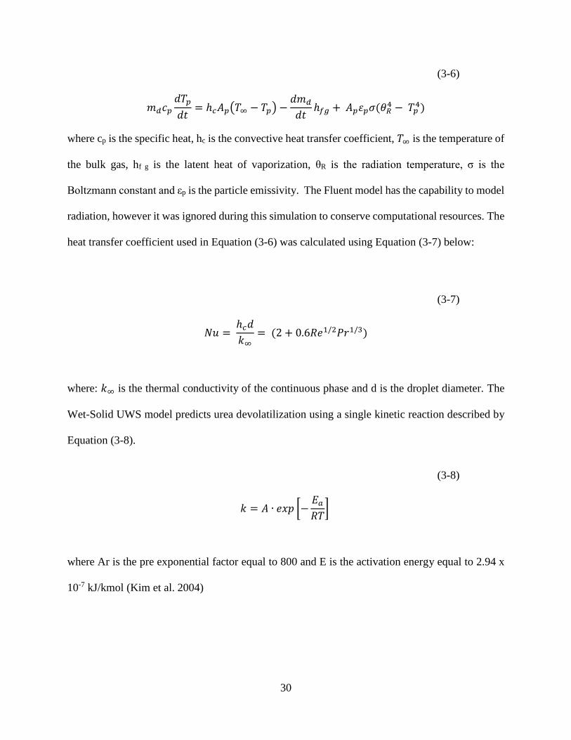
30

(3-6)

𝑚𝑑𝑐𝑝

𝑑𝑇𝑝

𝑑𝑡= ℎ𝑐𝐴𝑝(𝑇∞ − 𝑇𝑝) −

𝑑𝑚𝑑

𝑑𝑡ℎ𝑓𝑔 + 𝐴𝑝𝜀𝑝𝜎(𝜃𝑅

4 − 𝑇𝑝4)

where cp is the specific heat, hc is the convective heat transfer coefficient, 𝑇∞ is the temperature of

the bulk gas, hf g is the latent heat of vaporization, θR is the radiation temperature, σ is the

Boltzmann constant and εp is the particle emissivity. The Fluent model has the capability to model

radiation, however it was ignored during this simulation to conserve computational resources. The

heat transfer coefficient used in Equation (3-6) was calculated using Equation (3-7) below:

(3-7)

𝑁𝑢 = ℎ𝑐𝑑

𝑘∞= (2 + 0.6𝑅𝑒1/2𝑃𝑟1/3)

where: 𝑘∞ is the thermal conductivity of the continuous phase and d is the droplet diameter. The

Wet-Solid UWS model predicts urea devolatilization using a single kinetic reaction described by

Equation (3-8).

(3-8)

𝑘 = 𝐴 ∙ 𝑒𝑥𝑝 [−𝐸𝑎

𝑅𝑇]

where Ar is the pre exponential factor equal to 800 and E is the activation energy equal to 2.94 x

10-7 kJ/kmol (Kim et al. 2004)

31

3.6 One-Dimensional Catalytic Reaction Model

ASNSY Fluent 14.5 does not currently have a built-in capability to model the reaction kinetics that

occur in the catalyst portion of an SCR. As a result, a separate model was used to evaluate the

performance of the SCR using the CFD catalyst inlet conditions. An overview of the modelling

approach used is shown in Figure 3-6.

Figure 3-6: Overall SCR Modeling (Faltsi & Mutyal 2012).

The SCR catalyst is composed of several small channels, approximately 1 mm in cross sectional

length. Each of these channels has a monolith structure supporting a Vanadium Titania catalyst

that interacts with the NOx. Above the catalyst is a porous media or wash coat that guides the NH3

laced exhaust gas onto the catalyst surface. This particular type of catalyst is referred to as

selective as it only absorbs NH3 resulting in only the oxidation of NOx (Depcik & Assanis 2005).

These catalyst properties allow us to make the follow assumptions for modeling (Na 2010):

32

Individual channels are geometrically identical

Negligible heat loss conducted through catalyst walls, as all channels are close in

temperature

Flow in channels is assumed to be 1-dimensional and laminar, as the channels are small

and have Reynolds Numbers in the laminar regime

Flow is fully developed

NO2 concentration is negligible

Gas phase chemical reactions are negligible.

Ideal gases

Heat generation from NO conversion is negligible, as less than 0.001% of the exhaust gas

is comprised of ammonia and convective heat transfer is much more dominant.

Operational temperatures are always greater than 250oC. The SCR process breaks down

at temperatures lower than this.

The Eley-Rideal Mechanism governs the interaction of ammonia with the catalyst surface and has

been experimentally verified to apply between 250oC and 400oC (Nova et al. 2006). There are 4

dominant interactions with that the catalyst and ammonia gas; these are described below:

Absorption (Ra), Ammonia molecules are absorbed onto the catalyst surface.

Desorption (Rd), Previously absorbed ammonia is released from the catalyst surface.

Reduction (Rr), Absorbed ammonia interacts with NO gas.

Oxidation (Ro), Absorbed ammonia reacts with Oxygen in exhaust gas.

The chemical formulas that apply to the Eley-Rideal interactions are:

33

(3-9)

(Ra) NH3(g) NH3(s)

(3-10)

(Rd) NH3(s) NH3(g)

(3-11)

(Rr) 4NH3(s) + 4NO(g) + O2(g) 6H2O(g) + 4N2(g)

(3-12)

(Ro) 4NH3(s) + 3O2(g) 2N2(g) + 6H2O(g)

The rates of the reactions outlined in Equations (3-9) through (3-12) can be described by the

Arrhenius Equation shown in Equation (3-13).

(3-13)

𝑘 = 𝐴 ∙ 𝑒−𝐸𝑎/(𝑅𝑇)

where k is the rate constant of the reaction, A is the pre-exponential factor, Ea is the Activation

Energy, and R is the Universal Gas Constant. Catalyst manufacturers do not publish the rate

constants and pre-exponential factors associated with their products, so experimental values were

used from the literature (Chatterjee et al. 2005).

Combining the Eley-Rideal Catalyst Mechanism with the Arrhenius Rate Equations allows the

derivation of differential equations that describes the SCR process. In total, five equations are

required to close the SCR system utilizing the assumptions outlined in the beginning of this

34

section. Equations (3-14) and (3-15) were derived by applying Conservation of Energy over the

respective wall and gas portions of the catalyst:

(3-14)

𝜕𝑇𝑔

𝜕𝑥= −

ℎ𝑐 ∙ 𝑃

𝜌𝑔𝐴𝑔𝑐𝑝,𝑔𝑈(𝑇𝑔 − 𝑇𝑤)

(3-15)

𝜕𝑇𝑤

𝜕𝑡= −

ℎ𝑐 ∙ 𝑃

𝜌𝑤𝐴𝑤𝑐𝑝,𝑤(𝑇𝑤 − 𝑇𝑔)

where: Tg is the temperature of the gas, P is the pressure, ρg is the density of the gas, Ag is the cross

sectional area of the catalyst wall, cp,g is the specific heat of the gas, U is the axial velocity, Tw is

the temperature of the gas at the wall, ρw is the density of gas at the wall and cp,w is the specific

heat of gas at the wall. Equations (3-16) and (3-17) were derived by applying the law of mass

conservation to the respective NH3 and NO species, these equations are listed below:

(3-16)

𝜕𝐶𝑁𝐻3

𝜕𝑥=

𝑠

𝐴𝑔𝑈[−𝑝𝑎(1 − 𝜃)𝐶𝑁𝐻3 + 𝑝𝑑exp (−

𝐸𝑎 𝑑(1 − 𝛼𝜃)

𝑅𝑇𝑤)𝜃]

(3-17)

𝜕𝐶𝑁𝑂

𝜕𝑥=

𝑠

𝐴𝑔𝑈[−𝑝𝑟exp (

𝐸𝑎 𝑟

𝑅𝑇𝑤)𝜃𝐶𝑁𝑂]

where, s the number of molecular storage sites per axial meter, C is the concentration of the

corresponding species, pa is the pre-exponential factor for absorption, pd is the pre-exponential

factor for desorption, Ea d is the activation energy of the desorption reaction, Ea r is the activation

35

energy of the reduction reaction, θ is the fraction of ammonia storage and α is the molar feed ratio

of ammonia.

along the direction of flow in a channel. Equation (3-18) is also derived by applying the law of

mass conservation to the ammonia absorbed on the catalyst (θ) and is shown below:

(3-18)

𝜕𝜃

𝜕𝑡= [𝑝𝑎(1 − 𝜃)𝐶𝑁𝐻3 − 𝑝𝑑 exp(−

𝐸𝑎 𝑑(1 − 𝛼𝜃)

𝑅𝑇𝑤)𝜃 − 𝑝𝑟 exp (−

𝐸𝑟

𝑅𝑇𝑤) 𝜃𝐶𝑁𝑂

− 𝑝𝑜exp (−𝐸𝑎,𝑜

𝑅𝑇𝑤)𝜃𝐶𝑂2]

where: Ea o is the activation energy of the oxidation reaction and po is the pre-exponential factor

for oxidation. Equations (3-14) through (3-18) were solved using a Matlab script developed by

Safety Power Inc (Safety Power Inc 2013).

This script uses Gear’s Algorithm to solve Equations (3-15) and (3-18) or the time dependent part

of the system. The built in Matlab ODE solver is then used to evaluate Equations (3-14), (3-16)

and (3-17) that reside in the spatial domain.

The catalyst was divided into 1,156 individual elements, as this was the number available from the

Fine Grid Resolution mesh CFD solution. More elements would increase the accuracy of the

analysis based on an asymptotic relationship outlined in Section 3.7 (Celik et al. 2008).

3.7 Numerical Error

ASME has defined a method to quantify discretization error, ensuring confidence in CFD results

(Celik et al. 2008). The ASME discretization error method uses both the Richardson Extrapolation

(RE) and the Fine Grid Convergence Index (GCI) methods. The ASME method have been used in

36

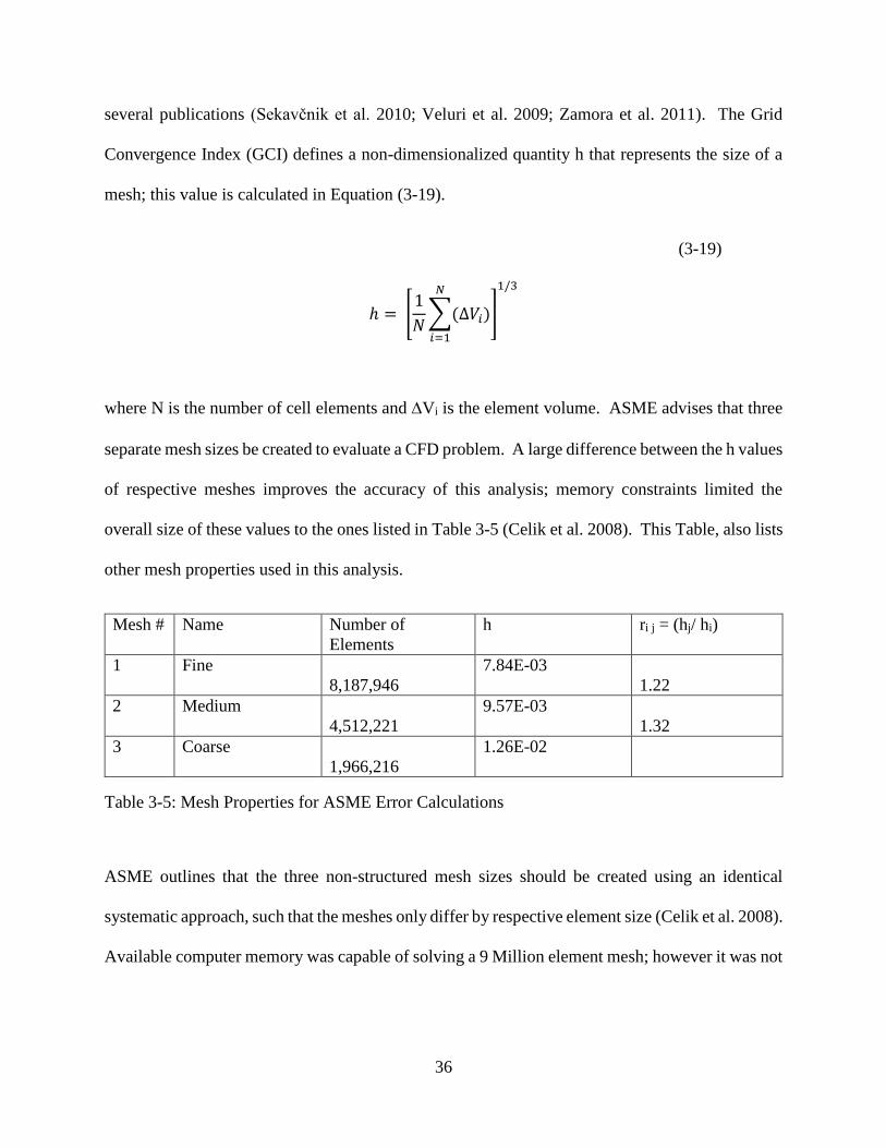
several publications (Sekavcnik et al. 2010; Veluri et al. 2009; Zamora et al. 2011). The Grid

Convergence Index (GCI) defines a non-dimensionalized quantity h that represents the size of a

mesh; this value is calculated in Equation (3-19).

(3-19)

ℎ = [1

𝑁∑(∆𝑉𝑖)

𝑁

𝑖=1

]

1/3

where N is the number of cell elements and Vi is the element volume. ASME advises that three

separate mesh sizes be created to evaluate a CFD problem. A large difference between the h values

of respective meshes improves the accuracy of this analysis; memory constraints limited the

overall size of these values to the ones listed in Table 3-5 (Celik et al. 2008). This Table, also lists

other mesh properties used in this analysis.

Mesh # Name Number of

Elements

h ri j = (hj/ hi)

1 Fine

8,187,946

7.84E-03

1.22

2 Medium

4,512,221

9.57E-03

1.32

3 Coarse

1,966,216

1.26E-02

Table 3-5: Mesh Properties for ASME Error Calculations

ASME outlines that the three non-structured mesh sizes should be created using an identical

systematic approach, such that the meshes only differ by respective element size (Celik et al. 2008).

Available computer memory was capable of solving a 9 Million element mesh; however it was not

37

possible to create a fine mesh this size without deviating from the systematic element size scaling

approach.

To satisfy both the ASME numerical error analysis and capture the inlet behaviour resulting from

the upstream DPF, the modeling was done in two parts:

1) The ASME numerical error analysis was performed on the SCR-only portion that is the

research focus of this analysis; the corresponding geometry is shown in Figure 3-7.

2) The resulting Medium SCR mesh from the ASME Error Analysis was combined with

the simplified DPF mesh from upstream DPF to capture an accurate SCR system inlet

profile. This mesh is utilized to evaluate the final results presented in this thesis.

Figure 3-7: Geometric Configuration of SCR Only Design

The smallest SCR-only mesh, outlined in Table 3-5 is approximately 2 million elements; adding

the DPF section to the SCR creates a coarse mesh of approximately 6.5 million elements.

38

Performing the ASME numerical error analysis on this complete SCR and DPF mesh would

require a fine mesh with of over 30 million elements (Celik et al. 2008). Given the memory

constraints described above it was not computationally possible to solve a mesh of this size for

this research project and as a result the SCR-only mesh was created.

The numerical error process uses the Equations (3-20) through (3-22) to determine the apparent

order, p of the discretization method:

(3-20)

𝑝 = 1

ln (𝑟21)|𝑙𝑛 |

𝜀32

𝜀21| + 𝑞(𝑝)|

(3-21)

𝑞(𝑝) = ln (𝑟21

𝑝 − 𝑠

𝑟32𝑝 − 𝑠

)

(3-22)

𝑠 = 1 ∙ 𝑠𝑔𝑛(𝜀32

𝜀21)

where 𝜀32 = ∅3 − ∅2; 𝜀21 = ∅2 − ∅1 and ∅𝑖 is respective solution point of interest of the ith size

mesh. The mesh sizes are labeled from 1 to 3 with 1 representing the fine mesh size and 3

representing the coarse mesh size.

Equations (3-20) through (3-22) were solved iteratively until a converged solution was achieved.

The final value of p was then used to determine the extrapolated exact solution of the CFD model

(referred to as the extrapolated value), using Equation (3-23):

(3-23)

∅𝑒𝑥𝑡21 =

𝑟21𝑝 ∅1 − ∅2

𝑟21𝑝 − 1

39

The goal of SCR design is to create a constant distribution of NH3 and exhaust gasses across the

catalyst face. Most research utilizes CFD to determine these properties and then utilize a separate

1-D analysis to evaluate overall SCR performance and NOx reduction (Pong et al. 2012; Depcik

& Assanis 2005). The quantities for axial velocity, static pressure and NH3 concentration were

sampled across the horizontal mid plane of the catalyst face. The results of this process are shown

in Figure 3-8 through Figure 3-10. Please note that H2O concentration was used in this analysis to

represent NH3.

Figure 3-8: Extrapolated Value of Axial Velocity across Catalyst Face

40

Figure 3-9: Extrapolated Value of NH3 Concentration across Catalyst Face

Figure 3-10: Extrapolated Value of Static Pressure across Catalyst Face

Overall the extrapolation yields solutions consistent with the Fine Mesh Solution. The largest

deviation was 9.5 % or 0.028% concentration by volume of NH3 occurring at a lateral position of

approximately 1.0 m. The average difference in extrapolated values across the Axial Velocity,

41

NH3 Concentrations and Static Pressure plots was 0.49% deviation from the Fine Mesh Solution.

Aside from the injection, all other values were determined to be well within acceptable errors

The RE Method that is utilized in the above figures has some inherent errors. These errors are

highlighted in Figure 3-8 and Figure 3-10, in the regions where the extrapolated values peak or

deviate from the fine grid solutions.

The 6 points in Figure 3-9 where there is an apparent deviation between the Extrapolation and Fine

Mesh solutions can be explained by examining Equation (3-23). This equation breaks down when

the value of 𝑟21𝑝

approaches one, resulting in a solution that approaches infinity. All 6 points where

deviation is observed, produce a 𝑟21𝑝

close to one. One of the underlying assumptions in using

the RE Method is for a solution in the asymptotic range. This error is likely the result of the solution

deviating from the asymptotic range. Fortunately, these deviations occur infrequently and result

in a small overall effect on the results (Celik et al. 2005).

The ASME Error Uncertainty Method uses the following approach to solve the Fine Grid

Convergence Index (GCIfine):

(3-24)

𝑒𝑎21 = |

∅1 − ∅2

∅1|

(3-25)

𝐺𝐶𝐼𝑓𝑖𝑛𝑒21 =

1.25𝑒𝑎21

𝑟21𝑝 − 1

42

Below are identical representations of numerical error for the Axial Velocity, NH3 Concentration

and Static Pressure across the face of the catalyst. The error is shown in the form of error bars on

top of the fine grid solution.

Figure 3-11: GCIfine with Error Bars of Axial Velocity across Catalyst Face

Figure 3-12: GCIfine with Error Bars of NH3 Concentration across Catalyst Face

43

Figure 3-13: GCIfine with Error Bars of Static Pressure across Catalyst Face

Similar to the RE results, Figure 3-11 through Figure 3-13 have a small numerical error. The

average error across the Axial Velocity, H2O Concentration and Static Pressure is 0.63%. The

maximum error is 13.16% and occurs at the exact same point as the highest deviation in the RE

method. This error is small and is equal to an overall 0.028 % difference in NH3 concentrations

by volume. Since the GCI method is based on the Richardson Expansion, the same points where

𝑟21𝑝

approaches one are attributed to higher error. This breakdown of the model is one of the

limitations of the RE method and allows these individual predicted values to be neglected (Ferziger

& Peric 1996).

Overall the numerical error identified from both the Richardson Expansion and GCIfine methods

are less than 1%. This indicates that the mesh size and orientation have been appropriately selected

as they yield acceptable numerical error. Low error in these critical design variables indicates low

numerical error in the overall SCR and NOx reduction process.

44

The method also recommends that convergence be achieved with 4th order residuals. All numerical

solutions presented in this thesis have achieved this level of convergence, with the exception of

computations involving an injection. Injecting species into the solution introduces an additional

source of mass that affects the convergence of the continuity equation. To minimize this effect,

the injection is performed on a small time scale, this yields residuals that approximate 4th order.

Below is a plot of the fine grid solution residuals.

Figure 3-14: Residual Plot for Fine Mesh with Injection

45

4 Results and Discussion

The computational modeling methodology outlined in Chapter 3 has been used to evaluate an HEV

only mixer, a U-bend only mixer and a combined HEV and U-bend design. These simulations

were chosen to isolate the performance of the individual mixing components so that the associated

contribution to performance could be identified. Due to the large computational expense

associated with fully modeling these components a simplified water spray simulation was selected.

The water spray simulation is well suited to compare overall bulk mixing trends. A full single

injection rate, urea water spray simulation was then used to evaluate the final design. A

comparison between the results of the water spray and full single rate model has also been made.

The 1-D model outlined in Section 3.6 was then employed to predict the final NOx reduction and

NH3 slip of the overall design.

4.1 HEV Model

The HEV mixer was modeled separately to identify the individual effect of this component on

performance and to establish a suitable mixing length. A long mixing length is ideal as it will

generate a high degree of mixing, but is not spatially practical for a U-bend type design. The

desired mixer is one that generates a fair degree of mixing with the least spatial impact on the

overall U-bend design.

46

Figure 4-1, shows the geometry used to evaluate the HEV only model. Flow enters at the far end

located by the mixing vanes, an injection point then occurs, flow then passes through the two sets

of mixing and a pressure outlet located 2.2 m downstream.

The injection point was selected at an axial distance of 30 cm before the first set of HEV vanes so

that the combined flow would have as ample time to interact with the mixing vanes. To evaluate

mixing performance and mixing distance, the injected water spray UI was sampled at measurement

slices in 0.1 m axial increments after the mixing vanes. Contours of the water spray injection are

shown in Figure 4-1. Initially the modeled water spray concentrations are highly concentrated in

the center of the mixing tube. The effectiveness of the HEV mixer is demonstrated by the relatively

even water spray concentration near the end of the mixer.

Figure 4-1: HEV Only Mixer

47

The full performance of the HEV only mixer is shown in, Figure 4-2. The performance is

measured by taking the UI of the axial velocity and water spray concentrations at the measurement

slices. The UI for velocity and spray concentrations peak at the end of the tube at 97.8% and

96.8% respectively. It was observed that the modeled UI performance increases at a high rate until

a mixing length of 0.7 m. After 0.7 m, the overall increase in UI is gradual. As a result, a 0.7 m

mixing length was selected for the overall combined HEV mixer and U-bend design. The

corresponding UI of velocity and water spray at 0.7 m are 93.2% and 93.4% respectively.

Figure 4-2: HEV Mixer Full Load Performance

Pressure loss is a major concern with the SCR design. Figure 4-3, represents a mid-plane contour

plot of the overall HEV mixer. A pressure loss of 805 Pa or 3.31” WC was predicted across the

mixing vanes. This pressure loss was calculated by taking the difference between the mass

averaged cross-sectional value at the inlet and after the second set of vanes. Little pressure loss

0.5

0.55

0.6

0.65

0.7

0.75

0.8

0.85

0.9

0.95

1

0.1 0.3 0.5 0.7 0.9 1.1 1.3

UI

Distance (m)

HEV Mixer, UI Vs. Mixing Length

Velocity

H2OInjection

48

was predicted after the second set of vanes; the associated pressure loss was calculated to be 13 Pa

or 0.05 “ WC. This indicates that the overall length downstream of the mixing tube has little effect

on overall pressure loss.

Figure 4-3: Mid-Plane Total Pressure Contour Plot of HEV Only Mixer

Effective mixing performance under partial loading conditions was a goal of this work.

Performances metrics were utilized to evaluate the UI of water spray concentrations at 45% and

10% loads. The corresponding UI was calculated to be 89.1% for both loading conditions; Figure

4-4, presents the results. This represents a 4.3% reduction in UI at these loading conditions. Partial

loading UIs are critical to the overall design, this partial loading performance degradation is an

important design limitation that will be address further in Section 4.2.

49

Figure 4-4: HEV Mixer, Water Spray Partial Loading Performance

4.2 HEV and U-bend Performance

The geometry in Figure 3-1 was used to model the performance differences between a U-bend

only mixer and a combined HEV and U-bend mixer. In the U-bend only design, the mixing vanes

were treated as interior space instead of walls, resulting in an identical geometric model except

without the vanes. Pathlines were utilized to display the overall similarities and differences

between the two models. The U-bend only and combined models are shown in Figure 4-5 and

Figure 4-6, respectively. Colours are utilized to represent the starting position of individual

pathlines. Both of these models are evaluated at full load performance. Overall these two designs

produce similar flow patterns. The major difference is emphasized in the magnified HEV mixer

section shown in Figure 4-6, where pathlines mix as shown by the greater distribution of colours

near the end of the HEV mixer. This increased mixing aligns with the findings of the HEV only

mixer shown in Section 4.2.

0.5

0.55

0.6

0.65

0.7

0.75

0.8

0.85

0.9

0.95

1

0.1 0.3 0.5 0.7 0.9 1.1 1.3

UI

Distance (m)

HEV Mixer, UI Vs. Mixing Length

100% Load

45% Load

10% Load

50

Figure 4-5: Pathlines for Full Load U-Bend Model

Figure 4-6: Pathlines for Full Load Combined HEV and U-Bend Model

As discussed in Section 3.7, the most important metric to determine the effectiveness of an SCR

system is the molar concentration of the injectant at the face of the catalyst. The ideal profile would

have a constant molar feed ratio (α) equal to one, indicating that the proportion of NOx is equal to

51

that of NH3. The molar feed ratios for both the U-bend only and combined HEV and U-bend

designs are shown in Figure 4-7 and Figure 4-8 respectively with the vertical scale for α kept

constant. Comparing the shape of the profiles it is evident that the addition of the HEV mixer

improves performance by creating a much flatter profile that better approaches the ideal case. This

is illustrated by examining the local minimum and maximum values of both graphs. In Figure 4-7

the maximum molar feed ratio is 1.3417 and the minimum is 0.65083; in Figure 4-6 the maximum

is 1.19862 and the minimum is 0.79868. Both of the values in the combined HEV and U-bend

design are closer to one indicating a more even distribution.

Figure 4-7: U-bend Only Model, Molar Feed Ratio across Catalyst

52

Figure 4-8: Combined HEV and U-bend Model, Molar Feed Ratio across Catalyst

The performance increase is further analyzed by examining the UI for velocity and water spray

across the catalyst face. The modeled water spray UI for the U-bend only and combined design

are 93.6% and 97.8% respectively. The addition of the HEV mixer increases the overall full load

UI by 4.2%; a substantial increase in performance. The velocity UIs for the two models are 98.0%

and 97.3% respectively, representing a 0.7% decrease in modeled performance. This slight

decrease in the overall velocity profile is caused by the HEV mixing effect observed in Section

4.1.

The overall impact in NOx reduction can be approximated by evaluating the UI of the molar feed

ratio α. The UI of the molar feed ratio is evaluated utilizing the resulting data obtained by

multiplying the normalized water concentration by the normalized axial velocity profile across the

catalyst face. The increase in molar feed ratio UI resulting from the combined HEV and U-bend

design is equated at 3.4%. The overall molar feed ratio UI for this design was calculated to be

95.7%. This means that this model predicts a theoretical full load NOx conversion level of 95.7%.

This helps show that the increase in water spray UI outweighs the decrease in velocity UI. The

values are theoretical as they do not include catalytic reactions; it also assumes that the injection

53

flow has a negligible physical influence on overall bulk exhaust flow. Section 4.3 calculates the

overall NOx reduction with a model that includes these variables.

A 2.3” WC increase in pressure drop was predicted using the combined HEV and U-bend design.

The combined design model produces a total pressure drop of 7.7” WC, representing a 42%

increase over the U-bend only design. This pressure drop level is well below the design target of

10” WC. An overall increase in pressure drop is expected as the increased mixing process

dissipates energy.

Partial loading conditions were evaluated with the water spray model. Table 4-1, displays the

partial loading velocity and water spray UIs. All calculated UI values are above the thesis design

goal of 97%. This is particularly interesting as a notable decrease in performance was observed at

lower loads using the HEV only design with the same mixing tube length. This decreased in

performance was does not exist in Table 4-1, indicating that the U-bend was able to compensate

for this variation

Load UI of H2O

UI of

Velocity

100% 97.8% 97.3%

45% 97.5% 97.0%

10% 97.6% 98.0%

Table 4-1: Partial Loading Performance of Combined HEV U-bend Design

4.3 NOx and NH3 Results from UWS Simulation

A single rate based urea water solution model was used to model the full load performance of the

combined HEV and U-bend design. Figure 4-9, is a contour plot showing the mid-plane velocity

magnitude. The velocity significantly increases in the HEV mixer area, as a result of the smaller

54

diameter and flow obstructions caused by the mixing vanes. A recirculation area is identified by

a zero velocity magnitude. This recirculation zone is responsible for the mixing action of the U-

bend, causing the flow to become relatively uniform across the catalyst surface.

Figure 4-9: Mid-Plane Contour Plot of Axial Velocity

A similar mid-plane contour for the total pressure is shown in Figure 4-10. As discussed in the

HEV only model, pressure decreases substantially across the HEV mixer. There is also a fairly

large pressure loss at the beginning of the catalyst region; this makes sense as the porous nature of

the catalyst is more resistant. The total pressure drop utilizing UWS model was calculated at 7.8”

WC, which represents a 1.3% difference from the water spray model.

55

Figure 4-10: Mid-Plane Contour of Total Pressure

Temperature loss was evaluated using the Fluent outer wall convective heat loss model (ANSYS

2012). The outside free stream temperature was set to 250 K so that the thermal loss was evaluated

under extreme winter conditions. Less heat loss would occur in more realistic operating conditions

as there would be less of a temperature difference between the outside air and the exhaust stream.

The outside walls were modeled with the conductive properties of 2.5 mm thick stainless steel.

Figure 4-11 represents a mid-plane contour of the temperature throughout the SCR design. An 18

K loss of temperature was predicted over the whole SCR. This temperature loss equates to 48.1

kW of heat loss to the surroundings. This heat loss has a small effect on the overall flow field, as

it represent a 4.0% heat loss when compared to the overall 1,202 kW of thermal energy passing

through the SCR.

56

Figure 4-11: Mid-Plane Contour Plot of Temperature

Urea was injected into the SCR at an axial distance of 30 cm before the first set of HEV mixing

vanes. The full load injection rate was 0.00366 kg/s of the urea solution. Figure 4-12 represents

a mid-plane contour plot of the HNCO concentrations across the SCR. HNCO concentrations

increase near the beginning of the injection point as the 32 μm urea droplets are quickly evaporated

by the 700 K exhaust gas. The total HNCO concentration peaks at the beginning of the catalyst.

The HNCO decomposition that would occur through the catalyst is not shown as catalyst reactions

are modeled separately using the 1-D model. Figure 4-13 shows a mid-plane contour plot of the

NH3 concentration across the SCR. The NH3 concentrations are an order of magnitude higher than

the HNCO concentration; this aligns with Equations (2-7) through (2-9) as decomposition yields

double the amount of NH3. The lack of built in catalytic reactions in the model results in

continually climbing ammonia concentrations after the flow interacts with the porous catalyst.

Similar to the HNCO concentrations, this model is only valid up until the face of the catalyst.

57

Concentrations after this should be neglected as the separate 1-D reaction model was used to

evaluate the catalytic reactions.

Figure 4-12: Mid-Plane Contour of Full Load HNCO Concentrations

Figure 4-13: Mid-Plane Contour of Full Load NH3 Concentrations

58

The inputs to the 1-D catalyst reaction kinetics model are obtained from the urea water CFD

simulation. These model inputs are temperature, axial velocity, NH3 concentration and HNCO

concentration at each element on the catalyst face. Figure 4-14 shows the normalized axial

velocity across this face. The normalized axial velocity is calculated relative to the average axial

velocity over the entire catalyst face. The normalized velocity was bias towards the outer edge of

the U-bend and is symmetrical across the y-axis. The overall UI for the axial velocity was

determined to be 97.1%.

Figure 4-14: Normalized Axial Flow Velocity Across Catalyst Face

The urea water simulation yields concentrations for both NH3 and HNCO. Figure 4-15 displays

the normalized HNCO concentration across the catalyst face. This concentration like the velocity

profile has a bias towards the outer edge of the U-bend. The UI of the HNCO concentration was

predicted to be 93.1%. Figure 4-16 represents a contour plot of the normalized NH3 concentration

across the same face. As shown in Figure 4-13, NH3 concentrations are of an order of magnitude

higher than HNCO concentrations, making them much more influential on the final NOx reduction

result. The total UI of the NH3 across the catalyst face is 95.3%. The combined UI of HNCO and

59

NH3 across the catalyst is 95.0%. This represents a 2.8% reduction of the water spray analysis

conducted in Section 4.2.

Figure 4-15: Normalized HNCO Concentration Across Catalyst Face

Figure 4-16: Normalized NH3 Concentration Across Catalyst Face

The major difference between the water spray and UWS model is the urea decomposition time.

The water spray model simulates a droplet with a 100% water content resulting in a longer H2O

60

evaporation period. The model also assumes that all urea instantly becomes gaseous NH3 once the

H2O has been vaporized; this counteracts the previous increase by reducing the devolatilization

period.

The UWS model utilizes the actual 62.5% droplet water concentration while employing a rate

equation to describe the transition process of solid urea into NH3 gas. The result is that during a

narrow temperature band the decomposition periods of the two models are similar. Unfortunately,

it is difficult to take advantage of this narrow temperature band as engine temperatures are dictated

by engine type and loading conditions. During loading conditions below this temperature band,

the water spray model over-predicts urea decomposition times, the reverse occurs at higher

temperatures. Decomposition times impact the physical models that are employed. Specifically,

fully decomposed urea is treated as a fluid species instead of a discrete mass source. In this

particular full load simulation, the water spray analysis over-predicts the total urea decomposition

period (Birkhold et al. 2007).

The computational time required to evaluate the UWS model over the water spray model under

the full load conditions was an order magnitude higher. As established in Section 3.5, research

has shown that the UWS model is the most accurate model for predicting urea decomposition. The

2.8% performance difference between the two models enables the water spray model to be utilized

to evaluate the overall mixing trends of individual design features.

The 1-D model discussed in Section 3.6 was employed to evaluate the overall NOx reduction and

NH3 slip production at a diluted 15% O2 exhaust output. The urea injection rate was selected based

on 10 ppm of NH3 slip; higher injection rates reduce NOx further but generate more slip. This

value was selected as it was an initial design limitation.

61

The velocity, temperature, HNCO and NH3 concentrations on the catalyst face obtained from the

CFD simulation were used to evaluate the 1-D model. The final NH3 and NOx concentrations

using this model were determined to be 9.7 ppm and 26.6 ppm respectively based on 600 ppm NOx

engine exhaust. This ppm reduction results in 0.18 g/kWh of NOx production, a level well below

the Tier 4 target of 0.67 g/kWh (Pilusa et al. 2012). An engine producing 1200 ppm of NOx would

yield a total NOx output of 0.39 g/kW. This reduction demonstrates the effectiveness of the

combined HEV and U-bend design in achieving current and future regulations.

The use of the 1-D model was required to evaluate total NOx production as the UI of molar feed

ratio only provided a non-dimensioned representation of the mixing. Using this model, the overall

NOx conversion rate was predicted to be 91.8% before dilution.

The combined HEV and U-bend design produces a high degree of mixing with a water spray UI

of 97.8%. This represents a 3.4% increase in UI over the U-bend only design. To determine

overall NOx reduction the overall design was evaluated with a more accurate UWS model. The

UWS model yielded a 2.8% UI decrease, as the water spray model used a simplified urea

decomposition model. Pressure drop was also evaluated and determined to be less than the design

goal 10” WC. The final UWS results were evaluated using a 1-D catalyst reaction model. This

model yielded NOx reduction levels that meet current and future regulations. The result of

combining a HEV mixer with a U-bend is a success and should be utilized in future SCR design.

62

5 Conclusions and Recommendations

A 3-D CFD simulation with a water spray injection was used to evaluate three configurations: an

HEV only mixer, a U-bend only mixer and a combined HEV and U-bend design.

The HEV only mixer, delivered excellent performance measured using the UI of both water spray

and velocity at the exhaust outlet. Unfortunately, axial length limitations prevented the full extent

of this increased performance to be utilized in the combined HEV and U-bend design. The rate of

increase in UI dropped at an axial length of 0.7 m; as a result this length was utilized in the final

combined HEV and U-bend design. The pressure drop for the entire mixer was predicted to be

3.31” of water and varied little over the mixing length.

To evaluate the increased performance achieved with the combined HEV and U-bend design,

simulations were performed on both the combined and U-bend only geometries separately. The

combined design model yielded velocity and water spray UIs greater than the design goal of 97%.

Full load simulations also predicted a pressure drop of 7.7” of water, well below the design goal

of 10”. The molar feed ratio was used to evaluate the increased theoretical NOx conversion of

3.4% with the combined design. The combined design was also determined to have a fairly flat

performance profile under partial loading conditions. A 4.3% degradation in the UI was predicted

in partial loading conditions of the HEV only mixer; this decreased performance did not occur in

the overall combined HEV and U-bend design.

The combined HEV and U-bend design was also evaluated with a UWS model. The UWS requires

a substantial increase in computational expense and was used to evaluate full load conditions of

the final design. Overall, the general trends reflected what was seen in the water spray model

results. It was determined that the UWS model found a 2.3% lower NOx conversion rates. It was

63

also predicted that the overall SCR lost 48 kW or 4.0% of the total heat energy to the surroundings

while operating on a cold winter day.

NOx reduction and NH3 slip were evaluated using a separate 1-D reactions kinetics model. The

model used NH3 concentration, velocity and temperature inputs from the UWS model. The overall

NOx level and NH3 slip were modeled to be 26.6 ppm and 9.7 ppm respectively based upon an

engine with 600 ppm of NOx in the exhaust. This represents a 91.8% reduction before dilution

and generates NOx at levels well below the US EPA Tier 4 standard.

Overall, the addition of a HEV mixer to the U-bend design results in a 3.4% increase on modeled

mixing performance. Pressure drop is also increased by 2.3” WC but is still within the design

limitation of 10” WC. This combined mixing design creates an SCR design achieves the goals of

this thesis by ensuring current and future off-road emissions regulations can be met.

5.1 Future Recommendations

The design presented in this thesis has predicted excellent levels of NOx reduction. The next step

would be to create a scaled mock-up and perform measurements for comparison.

More complex models, such as transient RANS modeling and a Large Eddy Simulation (LES)

could be of use. Transient modeling would provide a better understanding of SCR during load

changes. This would be particularly interesting if this SCR design was ever utilized for non-power

generation applications. An LES simulation would provide a better understanding of the flow over

specific design features like the mixing vanes.

Another area of interest would be to integrate the catalyst reaction kinetics into the CFD

simulation. This integration would require extensive information from the catalyst providers so

64

that the detailed geometry could be reproduced. It would also require the integration of the catalyst

reactions into the solver. This could be done in Fluent using a user defined function or with an

Application Program Interface (API) to a commercial chemical kinetics software package.

Combining this type of modeling with transient conditions could create a more extensive model

that could be used under almost any operating condition.

Increasingly stringent regulations are always pushing the boundaries of off-road SCR design.

Future legislation will likely call for an even higher of NOx reduction requiring more enhanced

mixing. Creating an SCR that generates a higher level of mixing is achievable, but likely at the

expense of increased pressure drop. Large Diesel engines have a low tolerance for pressure drop

in the exhaust. The introduction of a fan to boost the static pressure could open a lot of doors and

new avenues of design, but at the cost of increased parasitic power consumption to drive the fan.

A 12,000 CFM fan would be required to handle the particular exhaust flow studied in this thesis.

Increasing the static pressure by 6” WC would require a 12 kW fan motor (Cincinnati Fan 2013);

this represents a 0.8% parasitic loss from the overall 1500 kW generator. Utilizing a fan would

have the advantage of creating a more space efficient design that could also reduce overall

production costs.

65

6 References:

USEPA. (2013). PART 1039—Control of Emissions from New and In-Use Nonraod

Compression Ignition Engines. U.S Government Printing Office (GPO). Retrieved August

05, 2013, from http://goo.gl/NMUYcJ

ANSYS. (2012). ANSYS FLUENT Theory Guide (Vol. 15317, p. 788).

Bakker, A., & Laroche, R. D. (2000). Modeling of the Turbulent Flow in HEV Static Mixers.

http://www.bakker.org/. Retrieved from http://www.bakker.org/cfmbook/cfmbook.htm

Berger, M. J., York, N., Aftosmis, M. J., Field, M., Berger, M., & Aftosmis, M. (1998). Aspects

(and Aspect Ratios ) of Cartesian Mesh Methods Aspects and Aspect Ratios of Cartesian

Mesh Methods. In 16th International Confernece on Numerical Methods in Fluid Dynamics

(p. 13).

Birkhold, F., Meingast, U., & Wassermann, P. (2006). Analysis of the Injection of Urea-water-

solution for automotive SCR DeNOx-Systems : Modeling of Two-phase Flow and. In SAE

2006 World Congress & Exhibition (p. 11).

Birkhold, F., Meingast, U., Wassermann, P., & Deutschmann, O. (2007). Modeling and

Simulation of the Injection of Urea-Water-Solution for Automotive SCR DeNOx-Systems.

Applied Catalysis B: Environmental, 70(1-4), 119–127. doi:10.1016/j.apcatb.2005.12.035

Celik, I. B., Ghia, U., & Roache, P. J. (2008). Procedure for Estimation and Reporting of

Uncertainty Due to Discretization in CFD Applications. Journal of Fluids Engineering,

130(7), 078001. doi:10.1115/1.2960953

Celik, I., Li, J., Hu, G., & Shaffer, C. (2005). Limitations of Richardson Extrapolation and Some

Possible Remedies. Journal of Fluids Engineering, 127(4), 795. doi:10.1115/1.1949646

Chatterjee, D., Burkhardt, T., Bandl-Konrad, B., Braun, T., Tronconi, E., Nova, I., & Ciardelli,

C. (2005). Numerical Simulation of Ammonia SCR-Catalytic Converters : Model

Development and Application. SAE transactions, 114(4), 437–448. Retrieved from

http://goo.gl/kc1GSB

Chatterjee, D., Weibel, M., Krutzsch, B., Koc, P., Nova, I., & Tronconi, E. (2008). Current

Status of Modeling Lean Exhaust Gas Aftertreatment Catalysts.. Advances in Chemical

Engineering, 33(07), 113. doi:10.1016/S0065-2377(07)33003-2

Cincinnati Fan. (2013). Cincinnti Fan Engineering Data. Manufacturer Catalog. Retrieved

October 10, 2013, from http://www.cincinnatifan.com/catalogs/EngData-203-internet.pdf

Cummins. (2013). Engine Specifications. Retrieved from http://goo.gl/kyWTiz

66

Depcik, C., & Assanis, D. (2005). One Dimensional Automotive Catalyst Modeling. Progress in

Energy and Combustion Science, 31(4), 308–369. doi:10.1016/j.pecs.2005.08.001

Eroglu, A., Dobbeling, K., Joos, F., & Brunner, P. (2001). Vortex Generators in Lean-Premix

Combustion. Journal of Engineering for Gas Turbines and Power, 123(1), 41.

doi:10.1115/1.1335481

Faltsi, R., & Mutyal, J. (2012). Confidence in Modeling SCR Aftertreatment Systems. In SAE

2006 World Congress & Exhibition (p. 40).

Fang, T., Coverdill, R. E., Lee, C. F., & White, R. a. (2008). Effects of Injection Angles on

Combustion Processes Using Multiple Injection Strategies in an HSDI Diesel Engine. Fuel,

87(15-16), 3232–3239. doi:10.1016/j.fuel.2008.05.012

Ferziger, J. H., & Peric, M. (1996). Further Discussion of numerical Errors in CFD. International

Journal for Numerical Methods in Fluids, 23(November 1994), 1263–1274.

Gröhn, A. J., Pratsinis, S. E., & Wegner, K. (2012). Fluid-Particle Dynamics During Combustion

Spray Aerosol Synthesis of ZrO2. Chemical Engineering Journal, 191, 491–502.

doi:10.1016/j.cej.2012.02.093

Helden, R. Van, Verbeek, R., Willems, F., & van der Welle, R. (2004). Optimization of Urea

SCR deNOx Systems for HD Diesel Engines Abstract Catalyst Configuration and Urea. In

SAE 2004 World Congress & Exhibition (Vol. 01, p. 13). Detroit, MI, USA: SAE

International. Retrieved from http://papers.sae.org/2004-01-0154/

Heywood, J. B. (2011). Internal Combustion Engine Fundamentals (3rd ed., p. 930). New York:

McGraw-Hill.

Hsieh, M.-F., & Wang, J. (2011). Sliding-Mode Observer for Urea-Selective Catalytic Reduction

(SCR) Mid-Catalyst Ammonia Concentration Estimation. International Journal of

Automotive Technology, 12(3), 321–329. Retrieved from

http://link.springer.com/content/pdf/10.1007%2Fs12239-011-0038-4

Jeong, S.-J., Lee, S.-J., & Kim, W.-S. (2008). Numerical Study on the Optimum Injection of

Urea–Water Solution for SCR DeNOx System of a Heavy-Duty Diesel Engine to Improve

DeNOx Performance and Reduce NH 3 Slip. Environmental Engineering Science, 25(7),

1017–1036. doi:10.1089/ees.2007.0224

Jiang, H., Lu, L., & Sun, K. (2011). Experimental Study and Numerical Investigation of Particle

Penetration and Deposition in 90° Bent Ventilation Ducts. Building and Environment,

46(11), 2195–2202. doi:10.1016/j.buildenv.2011.04.033

Kim, J. Y., Ryu, S. H., & Ha, J. S. (2004). Numerical Prediction on the Characteristics of Spray-

Induced Mixing and Thermal Decomposition of Urea Solution in SCR System. In

67

ICEFA04, 2004 Fall Technical Conferences of the ASME International Combustion Engine

Division (p. 6).

King, R. T. (2007). Design of a Selective Catalytic Reduction System to Reduce NOx Emissions

of the 2003 West Virginia University FutureTruck. West Virginia University. Retrieved

from http://goo.gl/Ih0GnB

Kuehlert, K., Webb, S., Schowalter, D., Holmes, W., Chilka, A., & Reuss, S. (2008). Simulation

of the Fluid–Structure-Interaction of Steam Generator Tubes and Bluff Bodies. Nuclear

Engineering and Design, 238(8), 2048–2054. doi:10.1016/j.nucengdes.2007.11.017

Kulmala, M., & Wagner, P. E. (1996). Nucleation and Atmospheric Aerosols 1996 (1st ed., p.

860). New York: Elesvier Science Limited.

Mansour, M. (2005). Pressure Drop of Segmented Reprinted From : Diesel Exhaust Emission

Control Modeling. In 2005 SAE World Congress (p. 11).

Na, H. (2010). Physics Based Modeling of Urea Selective Catalytic Reduction Systems. MIT.

Nova, I., Ciardelli, C., Tronconi, E., Chimica, D., Chimica, I., Milano, P., … Stuttgart, D.-.

(2006). NH 3 -SCR of NO over a V-based Catalyst : Low-T Redox Kinetics with NH 3

Inhibition. American Institue of Chemical Engineers, 52(9). doi:10.1002/aic

Oh, J., Kim, K., & Lee, K. (2012). Effects of Various Mixer Types on the Spatial Distribution of

a De-NOx Reductant. Fuel, 94, 93–101. doi:10.1016/j.fuel.2011.12.018

Pilusa, T. J., Mollagee, M. M., & E., M. (2012). Reduction of Vehicle Exhaust Emissions from

Diesel Engines Using the Whale Concept Filter. Aerosol and Air Quality Research, 12(1),

994–1006. doi:10.4209/aaqr.2012.04.0100

Pong, H., Wallace, J., & Sullivan, P. E. (2012). Modeling of Exhaust Gas Treatment for

Stationary Applications. In SAE 2012 World Congress & Exhibition (Vol. 01, p. 17). Det:

SAE International. doi:10.4271/2012-01-1300

Safety Power Inc. (2013). Safety Power, Non Linear SCR Catalyst Reactions Model (p. 9).

Mississauga.

Sekavcnik, M., Gantar, T., & Mori, M. (2010). A Single-Stage Centripetal Pump—Design

Features and an Investigation of the Operating Characteristics. Journal of Fluids

Engineering, 132(2), 021106. doi:10.1115/1.4000846

Shahraeeni, M., & Raisee, M. (2010). Investigation of Turbulent Mixed Convection of Air Flow

in Vertical Tubes Using a Zonal Turbulence Model. International Journal of Heat and

Fluid Flow, 31(2), 179–190. doi:10.1016/j.ijheatfluidflow.2009.12.004

Smith, C. R. (1990). United States Patent Number 4,929,088. United States.

68

Spraying Systems Co. (2013). Industrial Hydraulic Spray Products. Spraying Systems Co.

Catalog. Retrieved from http://www.spray.com/cat75/hydraulic/offline/download.pdf

Ström, H., Lundström, A., & Andersson, B. (2009). Choice of Urea-Spray Models in CFD

Simulations of Urea-SCR Systems. Chemical Engineering Journal, 150(1), 69–82.

doi:10.1016/j.cej.2008.12.003

Vahid, S. (2011). Development of Multi-Component Evaporation Models and 3D Modeling of

NOx-SCR Reduction System. Institut National Polytechnique de Toulouse. Retrieved from

http://ethesis.inp-toulouse.fr/archive/00001558/01/ebrahimian.pdf

Veluri, S. P., Roy, C. J., Ahmed, A., Rifki, R., Worley, J. C., & Recktenwald, B. (2009). Joint

Computational/Experimental Aerodynamic Study of a Simplified Tractor/Trailer Geometry.

Journal of Fluids Engineering, 131(8), 081201. doi:10.1115/1.3155995

Wang, T. J., Baek, S. W., Lee, S. Y., & Yeo, G. K. (2009). Experimental Investigation on

Evaporation of Urea-Water-Solution Droplet for SCR Applications. American Institue of

Chemical Engineers, 55(12), 3267–3276. doi:10.1002/aic

Xinqun, G., Dou, D., & Winsor, R. (2010). Non-Road Diesel Engien Emissions and Technology

Options for Meeting Them. In Agricultural Equipment Technology Conference (pp. 1–25).

Zamansky, V. M., Lissianski, V. V, Maly, P. M., Ho, L., Rusli, D., & Gardiner, W. C. (1999).

Reactions of Sodium Species in the Promoted SNCR Process. Combustion and Flame,

117(4), 821–831. doi:10.1016/S0010-2180(98)00127-8

Zamora, B., Kaisere, A. S., Kling, U., Lucas, M., & Ruiz, J. (2011). Uncertainty Analysis in the

Numerical Simulation of the Air-Water Droplet Motion Through Drift Eliminators. Journal

of Fluids Engineering, 133(9), 094501. doi:10.1115/1.4004762