Delivery Service through an Integrated Inventory ...ieomsociety.org/bogota2017/papers/202.pdf ·...

Proceedings of the International Conference on Industrial Engineering and Operations Management Bogota, Colombia, October 25-26, 2017

Delivery Service through an Integrated Inventory Management Model using a System Dynamics Model

P.Raghuram1, Mridula Sahay2 and P.G.Saleeshya3

1, 2 Department of Mechanical Engineering, Amrita School of Engineering

Amrita Vishwa Vidyapeetham University Coimbatore, T.N., India

2Amrita School of Business Amrita Vishwa Vidyapeetham University

Coimbatore, T.N., India Corresponding Author - [email protected], [email protected]

ABSTRACT A pull production system is a make-to-order environment where manufacturing is started only after customer order is received and hence demand is confirmed. In an environment having dominant flow path for the products, it offers challenging scope for the management and control of raw material, work-in-process and finished goods inventory. Literature and industrial practice suggests a variety of heuristic models used to control inventory to optimal levels. Estimating and knowing the current and future inventories to be maintained is essential to sustain the material flow throughout the planning period. In this paper, we develop an integrated inventory control model integrating the demand and component material flows in a multi-customer, multi-product environment using system dynamics simulation modeling. We have simulated the model in a pull production system where the complete cycle depends on the customer order. The inventory level and structure are linked to delivery service and in effect to competitive advantage.

Keywords Inventory Management, Delivery, system Dynamics

1. INTRODUCTIONInventory is a double-edged sword in the manufacturing world. When the capacity is not able to produce to

customer requirement, it is a boon; when things are flowing smooth, inventory is a waste of money (Verwater-Lukszo & Christina, 2005). Whatever the cost incurred, companies are expected to offer the right products at the right time in right quantities. Customized design and order fulfillment in a make-to-order system offers a day-to-day challenge in controlling inventory for the manufacturer. Stable demands, varying operation times, varying setup times, intermittent material flows, lack of transparent internal and external communication and high product mix are some of the characteristics of manufacturing which increase inventory (Minner, 2003). Two main objectives to be fulfilled are, primarily the level of inventory required to maximize customer order fulfillment, specified in terms of customer demand and finished goods inventory and secondly, the amount of in-process inventories specified in terms of flow of material and the amount of inventories must be able to keep up to the delivery service (Vastag & Montabon, 2001). Regulating the input flow on work released to production and the output flow to the customer based on the volume of work and flow times determines the trade-off between these two contradictory objectives. When the range of requirement is larger, the greater is the number of problems of investment, procurement, storage, holding, accounting, shortage and stock out deterioration (Wanke, 2010).

Inventory accumulation and management has been studied in isolation as a manufacturing domain problem rather than as a systemic domain problem (Angerhofer & Angelides, 2000). System dynamics (Forrester, 1958, 1997; Richardson, 2011) offers a platform to include the many variables of the system which affect the inventory. The model allows us to understand the feedback from each of the variables. In most realistic stock management situations, the complexity of the feedbacks among the variables precludes the determination of the optimal strategy (Sterman, 2000, 2001). The objective of this paper is to formulate a model to optimize the total system inventory by simulating a system dynamics (SD) model considering the systemic domain. The metrics used to optimize the SD model are customer order fulfillment and the actual amount of material inventories at the various stages, viz., raw materials, work-in-process and finished goods. The fundamentals of inventory management, system dynamics and various inventory models in system dynamics literature are briefly dealt with through a literature survey. We define the problem of inventory control in pull manufacturing and model formulation in SD. The simulation of the SD inventory model and the obtained results are also discussed.

© IEOM 748

mailto:[email protected]

mailto:[email protected]


2. LITERATURE REVIEW Considering the importance of inventory control, there is a vast amount of literature that deals with inventory

classification, inventory control and inventory reduction. There is a need to understand the factors affecting the three types of inventories, the conventional inventory control mechanisms and models, the framework of system dynamics modeling and the inventory models dealt with by the system dynamics literature.

2.1. Inventory Management

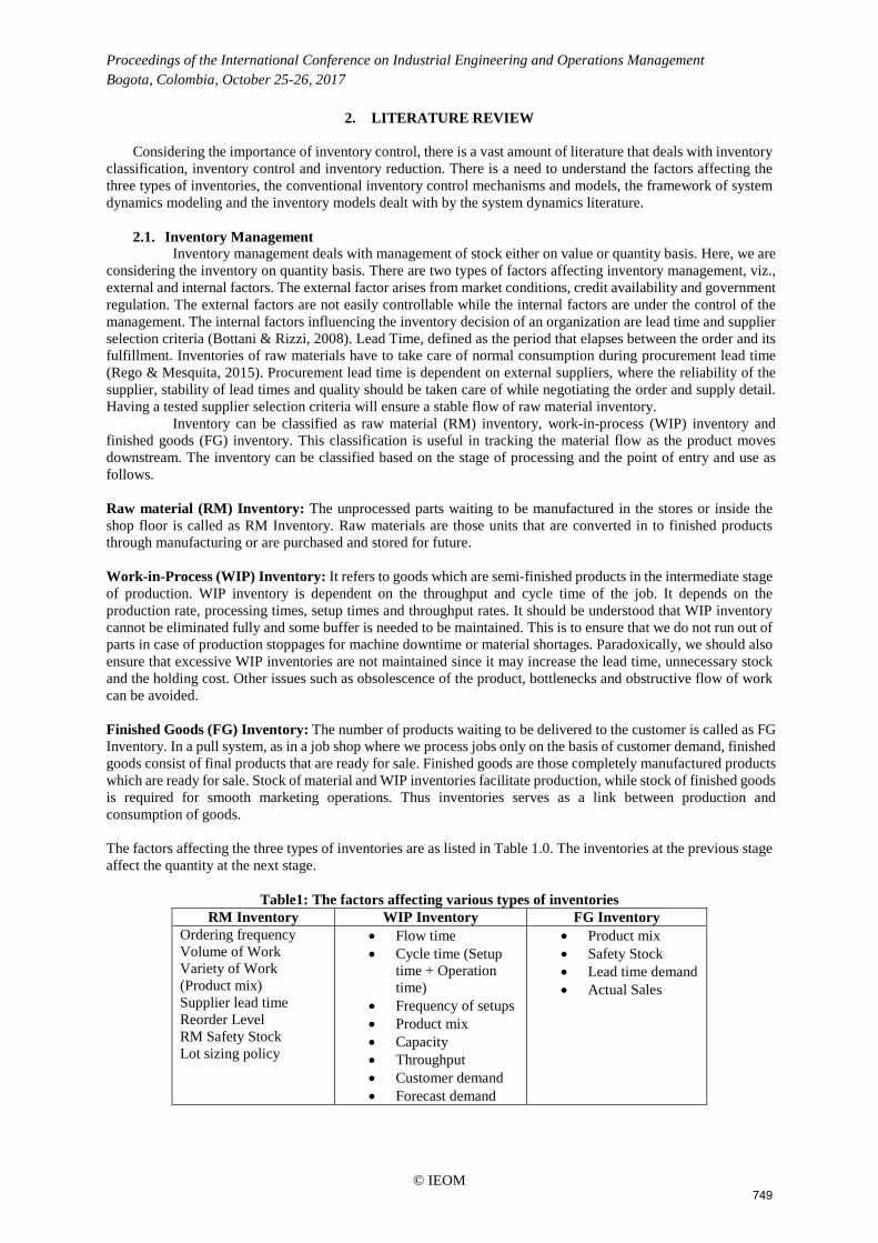
Inventory management deals with management of stock either on value or quantity basis. Here, we are considering the inventory on quantity basis. There are two types of factors affecting inventory management, viz., external and internal factors. The external factor arises from market conditions, credit availability and government regulation. The external factors are not easily controllable while the internal factors are under the control of the management. The internal factors influencing the inventory decision of an organization are lead time and supplier selection criteria (Bottani & Rizzi, 2008). Lead Time, defined as the period that elapses between the order and its fulfillment. Inventories of raw materials have to take care of normal consumption during procurement lead time (Rego & Mesquita, 2015). Procurement lead time is dependent on external suppliers, where the reliability of the supplier, stability of lead times and quality should be taken care of while negotiating the order and supply detail. Having a tested supplier selection criteria will ensure a stable flow of raw material inventory. Inventory can be classified as raw material (RM) inventory, work-in-process (WIP) inventory and finished goods (FG) inventory. This classification is useful in tracking the material flow as the product moves downstream. The inventory can be classified based on the stage of processing and the point of entry and use as follows. Raw material (RM) Inventory: The unprocessed parts waiting to be manufactured in the stores or inside the shop floor is called as RM Inventory. Raw materials are those units that are converted in to finished products through manufacturing or are purchased and stored for future. Work-in-Process (WIP) Inventory: It refers to goods which are semi-finished products in the intermediate stage of production. WIP inventory is dependent on the throughput and cycle time of the job. It depends on the production rate, processing times, setup times and throughput rates. It should be understood that WIP inventory cannot be eliminated fully and some buffer is needed to be maintained. This is to ensure that we do not run out of parts in case of production stoppages for machine downtime or material shortages. Paradoxically, we should also ensure that excessive WIP inventories are not maintained since it may increase the lead time, unnecessary stock and the holding cost. Other issues such as obsolescence of the product, bottlenecks and obstructive flow of work can be avoided. Finished Goods (FG) Inventory: The number of products waiting to be delivered to the customer is called as FG Inventory. In a pull system, as in a job shop where we process jobs only on the basis of customer demand, finished goods consist of final products that are ready for sale. Finished goods are those completely manufactured products which are ready for sale. Stock of material and WIP inventories facilitate production, while stock of finished goods is required for smooth marketing operations. Thus inventories serves as a link between production and consumption of goods. The factors affecting the three types of inventories are as listed in Table 1.0. The inventories at the previous stage affect the quantity at the next stage.

Table1: The factors affecting various types of inventories RM Inventory WIP Inventory FG Inventory

Ordering frequency Volume of Work Variety of Work (Product mix) Supplier lead time Reorder Level RM Safety Stock Lot sizing policy

• Flow time • Cycle time (Setup

time + Operation time)

• Frequency of setups • Product mix • Capacity • Throughput • Customer demand • Forecast demand

• Product mix • Safety Stock • Lead time demand • Actual Sales

© IEOM 749


2.2. Inventory Control In Manufacturing Inventory in the shop floor is maintained on the basis of departmental segregation. The different managers

maintain the inventory based on their individual calculations and judgment, and hence may result in interdepartmental dynamics, similar to the bullwhip effect across the supply chain. Centrally maintained inventories based on the customer order fulfillment will result in a better coordinated system. Having a systemic view of the inventories across departments will help the shop floor in decreasing the cost of the total inventories in the system. Optimal levels of the inventories throughout the material and operation flow will enhance the shop floor’s capacity to estimate and maintain accurate costs, remain flexible, improve responsiveness, optimize production capacity, track inventories and remain committed to customer orders.

In earlier periods, periodic inventory system was prevalent. Inventory used to be accounted for physically at the end of the year by taking stock and a physical verification of inventory is done. In this non-continuous system, it may not be possible to account for the calculation of work in process inventory. With the advent of computerized accounting system, purchases are entered immediately and point-of-sale records are maintained on a continuous basis. This ensures that the physical inventories and the inventories on record are the same any time of the year. This system of maintaining inventories is known as perpetual inventory system. In the perpetual inventory system, the calculation of inventory depends on the amount of purchases, current inventories and the shipments made and can be calculated easily. Of course, we assume that these entries are made correctly and also immediately. (Golini & Kalchschmidt, 2011; Kreng & Chen, 2007; Pejić-Bach & Čerić, 2007).

2.3. System Dynamics in Inventory Control

2.3.1. System Dynamics Developed by Forrester in 1961, system dynamics is a way of thinking about the system as a whole.

Instead of focusing on the discrete events, we need to move back deliberately and see the system as a whole for behavior patterns. System dynamics has created complex dynamic models and has affected policy decisions in the areas of climate change (Kunsch & Springael, 2008; Sahin et al., 2014), population control (Forrester, 1971), public policies (Sterman,2000; Wolstenholme,1983), environmental studies (Kaneko & Nojiri, 2008), social systems (Forrester, 1971), management (Warren & Langley, 1999; Zhang et al., 2012) and supply chain management (Angerhofer & Angelides, 2000; Masoumi et al., 2012). Selective abstractions of reality are used to construct mental models based on historical data and then test them on current data so that we can foresee futuristic results for different scenarios.

All dynamic systems are characterized by interdependence, mutual interaction, information feedback, and circular causality (Sterman, 2001). When we take decisions for individual events, it is called as reactive thinking; when we see the behavior patterns and adjust our approach accordingly, it is called as adaptive thinking; when we see the system as a whole and focus on policy decisions, it is called as systemic thinking. Having a systemic perspective helps us to perceive decisions as affecting not only the individual events, but the system as a whole (Thompson et al., 2014). Also, systemic structure affects the decisions we take decisions for events (Richardson, 2011). In effect, we can say that the performance of the system is dependent on the architecture of feedbacks and time delays. It is especially suited to inventory management since material flow as well as information flow has time delays. Feedback is an important aspect of system dynamics. Taking feedback from the system, systems thinking helps in redesigning the structure of the system. Feedback which causes the observed behavior is explicitly included in the system dynamics model. Using reinforcing and balancing loops of causality, it generates dynamic patterns of behavior (Sweeney & Sterman, 2000).

2.3.2. Inventory Control in System Dynamics Literature

Applied widely in the area of supply chain, system dynamics is well suited to the study of inventory management. The material flows and the effects of feedback can be studied in the context of inventory management and shipping policies. Feedback maintains the balance of the system or keeps it within limits and acts as a control mechanism. It usually dampens oscillatory behavior – stock-outs, long supply, or obsolete inventory items, for instance. Inventory flow is similar to a bathtub (Sterman, 2001) as water flows in at a certain rate, and exits through the drain at another rate. We can model and forecast the level of inventory based on the flow rates. Airline’s management of fuel inventory is usually found to be in excess to avoid stockouts which increases the cost of the inventories (Al-Refaie et al., 2010). This is similar to many manufacturing industries which maintain excess inventories in view of fluctuating demand requirements. Poles (2001) has explored closed loop supply chains in which the residence time of the product with the customer and customer behavior in returning the products is considered in increasing the efficiency in the management of inventories (Poles, 2001). In the next section, we formulate integrated inventory control model integrating the demand and component material flows in a multi-customer, multi-product environment that will ensure customer order fulfillment and delivery service requirements.

© IEOM 750


3. PROBLEM AND MODEL FORMULATION The model formulation approached through system dynamics modeling keeps track of the amount inventory

and work flow throughout the system as it is converted from raw material to finished goods. In this model, we are not using sale cash flows and purchase costs which are normally used in accounting. We also assume that the purchase of inventories is owned by the companies and are to be solely used for the manufacture of finished goods. Arrays are widely used throughout the model. The following arrays are defined in the hypothetical model. Customers are defined as ‘Customers’ dimension with three elements, products as ‘Products’ dimension with three elements, stock keeping unit as ‘SKU’ dimension with four elements, raw material inventory as ‘SKU Inv’ dimension with one element and safety stock as ‘SS’ dimension with one element. A hypothetical scenario is assumed to define the problem and can be summarized as follows.

Multiple products (three products, viz., Prod 1, Prod 2, Prod 3) are manufactured by a company. A number of customers (three customers, viz., Cust 1, Cust 2, Cust 3) are ordering varying volumes of the products. Here, it is assumed to be a steady demand throughout the year. Different monthly demands can also be incorporated into the model. The products are made of four parts, called as stock keeping units (SKU#1, SKU#2, SKU#3 and SKU#4) in the model. Varying combinations of the SKUs are required for each product. In this scenario, finished goods are manufactured to fulfill the customer orders. A maximum shipping limit is taken and the goods can only be delivered to the customer up to the maximum shipping. Safety stock of finished goods as well as raw materials is assumed. The raw material inventory (RM Inventory), work-in-process inventory (WIP Inventory) and finished goods inventory (FG Inventory) are to be calculated in this scenario. The resulting levels are tabulated along with graphs showing the time-variance of the inventories. A stock and level diagram, drawn using ISEE System’s iThink software v10.1.2, is used to represent the formulated problem and is described in detail along with the formulae used in the model in the following section.

3.1. Causal loop diagram The integrated inventory management model is depicted in the causal loop diagram shown in Fig.1.

3.2. Stock and Flow Diagram

The formulated inventory model is represented as a stock and flow diagram as shown in Fig. 2. These initial

values and the formulae are represented by the following sample equations, as shown through the description of the system dynamics model. Similarly, the other formulae are entered. The inventories of raw materials, work-in-process and finished goods at the end of each month is to be determined. The inventories at the end-of-year are found out and the flow of material can be tabulated, as shown in Table 1. These inventories are given initial values, as RM INVENTORY[SKU#], WIP INVENTORY[PRODUCT] and FG INVENTORY[PRODUCT].

Fig. 1. Causal loop Diagram for the Inventory model

Order Quantity

Desired RM Rate

FG saf ety stock

Desired Shipment

Order Fulf ilment

Ratio

Max Shipment

Desired Production

Desired RM

RM

Desired FG

Saf etyStock

CustomerOrder

Manuf acturingLead time

FG InvShip

FG Prodn RateWIP InvWIP Prodn RateUsed RM

RM Inv

RM

+

+

-

+ -

+

+

+

-

+

+

-

-

+

+

+

+

+

+

-

++

+

-

© IEOM 751


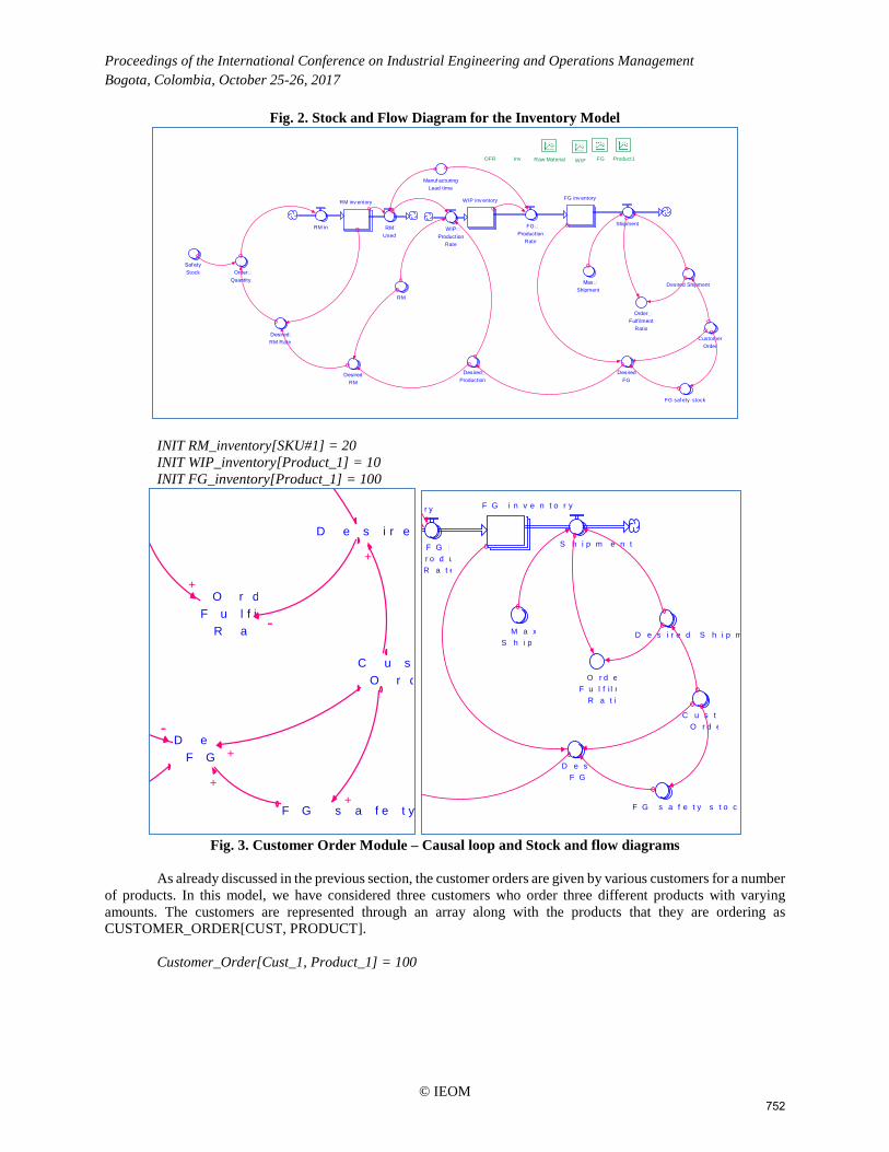
Fig. 2. Stock and Flow Diagram for the Inventory Model

INIT RM_inventory[SKU#1] = 20 INIT WIP_inventory[Product_1] = 10 INIT FG_inventory[Product_1] = 100

Fig. 3. Customer Order Module – Causal loop and Stock and flow diagrams

As already discussed in the previous section, the customer orders are given by various customers for a number

of products. In this model, we have considered three customers who order three different products with varying amounts. The customers are represented through an array along with the products that they are ordering as CUSTOMER_ORDER[CUST, PRODUCT].

Customer_Order[Cust_1, Product_1] = 100

RM inv entory

RM in

WIP inv entory FG inv entory

FG Production

Rate

Shipment

Order Quantity

Desired RM Rate

FG saf ety stock

Desired Shipment

Order Fulf ilment

Ratio

Max Shipment

Desired Production

Desired RM

RM

Desired FG

Saf ety Stock

CustomerOrder

RM Used

WIP Production

Rate

Manuf acturingLead time

WIP Product1Raw Material FGOFR Inv

F G s a f e t y

D e s i r e

O r dF u l f i

R a

D eF G

C u sO r d

+

+

+

-

+

+

-

r y F G i n v e n t o r y

F G r o d uR a t e

S h i p m e n t

F G s a f e t y s t o c

D e s i r e d S h i p m

O r d eF u l f i l m

R a t i

M a xS h i p

D e sF G

C u s t oO r d e

© IEOM 752


Table 2. Customer order for each product Customeer Product 1 Product 2 Product 3

Customer Order

Cust1 100 50 200 Cust 2 150 30 230 Cust 3 250 100 100

The customer order for each product is given as shown in Table 2 and are defined in the array as seen in

Fig. 3. Then the safety stock of finished goods, FG_SAFETY_STOCK[PRODUCT] is calculated and added for each product.

FG_safety_stock[Product_1] = .1*(Customer_Order[Cust_1, Product_1]+Customer_Order[Cust_2, Product_1]+Customer_Order[Cust_3, Product_1])

The customer orders and the safety stock can be added to get the desired number of finished goods, DESIRED_FG[PRODUCT]. Since we already have finished goods inventories, FG INVENTORY[PRODUCT], we need to subtract this from the desired number of finished goods.

Desired_FG[Product_1] = (Customer_Order[Cust_1, Product_1]+Customer_Order[Cust_2, Product_1]+Customer_Order[Cust_3, Product_1])+FG_safety_stock[Product_1]-FG_inventory[Product_1]

3.2.1. Raw Material Subsystem Loop The requirement of the finished goods is converted to the desired raw materials in the first subsystem, viz.,

the raw material subsystem loop, as shown in Fig. 4.

Fig. 4. Raw Material Subsystem Loop – Causal loop and Stock and flow diagrams

The finished goods requirement is passed on to DESIRED PRODUCTION[PRODUCT] and then is

converted into the number of raw material required, DESIRED RM[SKU#], which gives the number of stock keeping units (SKU#1, SKU#2, etc.) that are required.

Desired_Production[Product_1] = Desired_FG[Product_1] Desired_RM[SKU#1] = (Desired_Production[Product_1]*RM[Product_1,

SKU#1])+(Desired_Production[Product_2]*RM[Product_2, SKU#1])+(Desired_Production[Product_3]*RM[Product_3, SKU#1])

These values can be calculated from the array which gives the number of raw materials that are required to produce each product. Here, we require 3 units of SKU#1, 1 unit of SKU#2, 1 unit of SKU#3, and 2 units of SKU#4, and likewise for the other products. This is defined as

RM[Product_1, SKU#1] = 3 which can also be defined as shown in Table 3,

O r d eQ u a n

D e s iR M R

D e sR M

R M

S a fS t o

W U s e d R M

R M I n v

-

+ -

++

+

+

+

-

R M i n ve n t o r y

R M i n

W I P i n v

O r d eQ u a n t

D e s i rR M R

D e s i r eP r o d u c t

D e s i rR M

R M

S a f e tS t o c k

R MU s e

W IP P r o d u c

R a t e

M a n u fa c t uL e a d t im

O

© IEOM 753


Table 3. Stock keeping units (SKU#) requirement for each product

SKU Product 1

Product 2

Product 3

Raw Material

SKU#1 3 2 0 SKU#2 1 2 2 SKU#3 1 1 1 SKU#4 2 2 1

The desired raw material inventories, DESIRED_RM_RATE[SKU#] are then calculated taking into account

the currently available raw material inventories and subtracting them.

Desired_RM_Rate[SKU#1] = IF (RM_inventory[SKU#1]<Desired_RM[SKU#1] ) THEN Desired_RM[SKU#1] ELSE 0

The safety stock of each of the raw material, SAFETY_STOCK[SKU#, SAFETY_STOCK] is entered. Safety_Stock[SKU#1, Safety_Stock] = 20 The order quantity of each SKU, ORDER_QUANTITY[SKU#] can be calculated by adding the respective

safety stock, to that of the required raw materials. The safety stock is defined as an array, SS. Order_Quantity[SKU#1] = Desired_RM_Rate[SKU#1]+Safety_Stock[SKU#1, Safety_Stock] The raw material inventory, RM_INVENTORY[SKU#] is calculated from the rate of flow of raw materials,

RM_IN[SKU#] from the supplier. The variations that may be present in the supplier lead time or quantity are not taken into account, i.e., it is assumed that all the required parts are completely supplied. The raw materials are used to make the finished products according to the requirement of each product. Thus the raw materials that are used, RM_OUT[SKU#] is calculated as per the total requirement.

RM_in[SKU#1] = Order_Quantity[SKU#1] Manufacturing_Lead_time = 0.2 RM_Used[SKU#1] = RM_inventory[SKU#1]/Manufacturing_Lead_time RM_inventory[SKU#1](t) = RM_inventory[SKU#1](t - dt) + (RM_in[SKU] - RM_Used[SKU]) * dt 3.2.2. Work-in-process (WIP) Subsystem Loop The conversion of raw materials into finished goods consumes raw materials as per the requirements of the

products. This is then fed into the next loop, viz., WIP subsystem loop, shown in Fig. and the WIP inventory level, WIP_INVENTORY[PRODUCT] is calculated.

WIP_inventory[Product_1](t) = WIP_inventory[Product_1](t - dt) + (WIP_Production_Rate[Products] - FG_Production_Rate[Products]) * dt

The desired WIP, DESIRED_WIP[PRODUCT] is obtained from the number of finished goods that are required to be produced and the amount of in-process inventories, WIP_INVENTORY[PRODUCT] in the shop floor. The amount of WIP inventories, WIP_PRODUCTION_RATE[PRODUCT] that are produced are then fed into the finished goods inventories, FG_INVENTORY[PRODUCT].

WIP_Production_Rate[Product_1] = IF (RM_Used[SKU#1]/RM[Product_1, SKU#1])>Desired_Production[Product_1] THEN Desired_Production[Product_1] ELSE 0

Fig. 5. Work-in-process (WIP) Subsystem – Causal loop and Stock and flow diagrams

ManufacturingLead time

FG P rodn R aW IP InvW IP P rodn R ateU sed R M

R M

+

+ - -

+

y

W IP i n v e n t o ry

FG Pro d u c t i

Ra t e

RMUs e d

W IP Pro d u c t i

Ra t e

M a n u f a c t uL e a d t im e

a

© IEOM 754


3.2.3. Finished Goods (FG) Subsystem Loop As mentioned in the previous section, the WIP produced and stored as WIP inventories will give the rate at which the finished goods are produced, viz., FG_PRODUCTION_RATE[PRODUCT]. These are then stored as finished goods inventories, FG_INVENTORY[PRODUCT] in the finished goods subsystem loop, viz., FG Subsystem loop as shown in Fig.

FG_Production_Rate[Product_1] = WIP_inventory[Product_1]/Manufacturing_Lead_time FG_inventory[Product_1](t) = FG_inventory[Product_1](t - dt) + (FG_Production_Rate[Products] -

Shipment[Product_1]) * dt Shipment of these products depends on the desired shipment to customers, according to the customer orders.

The maximum shipment rate for each product, MAX_SHIPMENT[PRODUCT] is defined and shipment to the customer is done based on the minimum amount between the desired shipment, DESIRED_SHIPMENT[CUST, PRODUCT] and the maximum possible shipment.

Fig. 6. Finished Goods (FG) Subsystem – (a) Causal loop and (b) Stock and flow diagrams

Desired_Shipment[Cust_1, Product_1] = Customer_Order[Cust_1, Product_1] Max_Shipment[Product_1] = 500 Max_Shipment[Product_2] = 250 Max_Shipment[Product_3] = 400 Shipment[Product_1] = MIN(Max_Shipment[Product_1], Desired_Shipment[Cust_1,

Product_1]+Desired_Shipment[Cust_2, Product_1]+Desired_Shipment[Cust_3, Product_1]) The order fulfillment ratio, ORDER_FULFILMENT_RATIO can be calculated depending on the percentage

of customer orders delivered, i.e., actual shipment, to the orders placed by the customers and is limited by the maximum shipment possible for each product.

Order_Fulfilment_Ratio = ((Shipment[Product_1]/(Desired_Shipment[Cust_1,

Product_1]+Desired_Shipment[Cust_2, Product_1]+Desired_Shipment[Cust_3, Product_1]))+(Shipment[Product_2]/(Desired_Shipment[Cust_1, Product_2]+Desired_Shipment[Cust_2, Product_2]+Desired_Shipment[Cust_3, Product_2]))+(Shipment[Product_3]/(Desired_Shipment[Cust_1, Product_3]+Desired_Shipment[Cust_2, Product_3]+Desired_Shipment[Cust_3, Product_3])))*100/3

F G s a f e t y s

D e s i r e d

O r d eF u l f i l

R a t i

M a xS h i p

D e sF G

C u s tO r d e

F G I n vS h i p

G P r o d n R a t e

+

+

+

-

-

-

+

+

+

-

++

+

o r y F G i n v e n t o r y

F G P r o d u

R a t e

S h i p m e n t

F G s a f e t y s t o c k

D e s i r e d S h i p m

O r d eF u l f i l m

R a t i

M a xS h i p

D e sF G

C u s t oO r d e

© IEOM 755


Thus the stock and flow diagram is defined and then it is simulated using the system dynamics software, iThink v 10.1.2. The results of the simulation are discussed in the next section.

4. SIMULATION RESULTS AND DISCUSSION The inventory management model has been developed as described in the previous section. From the results

obtained, we can measure the level of inventories of the raw materials, i.e., the inventory levels of each SKU and the work-in-process inventories of each product as shown in Table and the finished goods inventories of each product as shown in Table 4. As the order

Table 4. Raw material (RM), Work-in-Process (WIP) and Finished Goods (FG) inventories Months

RM inventory[SKU#1]

RM inventory[SKU#2]

RM inventory[SKU#3]

RM inventory[SKU#4]

WIP inventory[Product 1]



FG inventory[Product 1]



Initial 20.00 30.00 40.00 50.00 10.00 10.00 10.00 100.00 200.00 50.00

1 346.43 347.55 222.00 350.07 100.00 23.81 97.88 50.78 62.11 118.83 2 371.31 343.92 220.92 360.61 99.94 33.76 83.24 50.23 26.10 171.28 3 375.14 342.36 220.17 361.75 99.99 35.59 80.59 50.04 19.49 180.85 4 375.84 342.07 220.03 361.95 100.00 35.92 80.11 50.01 18.27 182.61 5 375.97 342.01 220.01 361.99 100.00 35.99 80.02 50.00 18.05 182.93 6 375.99 342.00 220.00 362.00 100.00 36.00 80.00 50.00 18.01 182.99 7 376.00 342.00 220.00 362.00 100.00 36.00 80.00 50.00 18.00 183.00 8 376.00 342.00 220.00 362.00 100.00 36.00 80.00 50.00 18.00 183.00 9 376.00 342.00 220.00 362.00 100.00 36.00 80.00 50.00 18.00 183.00 10 376.00 342.00 220.00 362.00 100.00 36.00 80.00 50.00 18.00 183.00 11 376.00 342.00 220.00 362.00 100.00 36.00 80.00 50.00 18.00 183.00 12 376.00 342.00 220.00 362.00 100.00 36.00 80.00 50.00 18.00 183.00

Quantities change for each customer, the raw material inventories for the various SKUs are calculated. This

requirement is then compared to the available raw material inventories and then the needed quantities are purchased along with the safety stock. Graphs of the variation of different inventories, viz., Raw material inventories (Fig. 7), Work-in-process inventories (Fig. 8) and finished goods inventories (Fig. 9) have been plotted through the software to understand the variations of stock over the period.

10:28 AM Wed, Mar 2, 2016

Raw Material

Page 11.00 4.00 7.00 10.00 13.00

Months

1:

1:

1:

2:

2:

2:

3:

3:

3:

4:

4:

4:

0

200

400

0

150

300

0

200

400

1: RM inv entory [SKU#1] 2: RM inv entory [SKU#2] 3: RM inv entory [SKU#3] 4: RM inv entory [SKU#4]

1

1 1 12

2 2 2

3 3 3 3

4 4 4 4

© IEOM 756


Fig. 7. Raw material inventories of all products

Fig. 8. Work-in-process inventories of all products

Fig. 9. Finished goods inventories of all products

The inventories of raw materials and the resulting work-in-process inventories can also be plotted and these

inventories are shown in the graph plotted in Fig. 10.

10:28 AM Wed, Mar 2, 2016

WIP Inventory

Page 11.00 4.00 7.00 10.00 13.00

Months

1:

1:

1:

2:

2:

2:

3:

3:

3:

0

100

200

0

20

40

0

100

200

1: WIP inventory[Product 1] 2: WIP inventory[Product 2] 3: WIP inventory[Product 3]

1

1 1 12

2 2 2

33 3 3

10:28 AM Wed, Mar 2, 2016

Finished Goods Inv entory

Page 11.00 4.00 7.00 10.00 13.00

Months

1:

1:

1:

2:

2:

2:

3:

3:

3:

0

50

100

0

100

200

50

150

250

1: FG inv entory [Product 1] 2: FG inv entory [Product 2] 3: FG inv entory [Product 3]

1

1 1 1

2

2 2 2

3

3 3 3

© IEOM 757


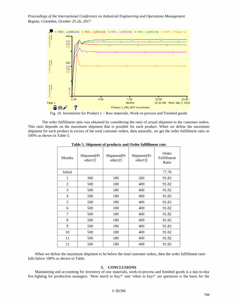
Fig. 10. Inventories for Product 1 – Raw materials, Work-in-process and Finished goods

The order fulfillment ratio was obtained by considering the ratio of actual shipment to the customer orders.

This ratio depends on the maximum shipment that is possible for each product. When we define the maximum shipment for each product in excess of the total customer orders, then naturally, we get the order fulfillment ratio as 100% as shown in Table 5.

Table 5. Shipment of products and Order fulfillment rate

Months Shipment[Product1]

Shipment[Product2]

Shipment[Product3]

Order Fulfillment

Ratio

Initial 77.76 1 360 180 260 91.82 2 500 180 400 91.82 3 500 180 400 91.82 4 500 180 400 91.82 5 500 180 400 91.82 6 500 180 400 91.82 7 500 180 400 91.82 8 500 180 400 91.82 9 500 180 400 91.82

10 500 180 400 91.82 11 500 180 400 91.82 12 500 180 400 91.82

When we define the maximum shipment to be below the total customer orders, then the order fulfillment ratio

falls below 100% as shown in Table.

5. CONCLUSIONS Maintaining and accounting for inventory of raw materials, work-in-process and finished goods is a day-to-day

fire-fighting for production managers. ‘How much to buy?’ and ‘when to buy?’ are questions is the basis for the

10:34 AM Wed, Mar 2, 2016

Product 1_RM_WIP Inv entories

.00 4.00 7.00 10.00 13.00

Months

1:

1:

1:

2:

2:

2:

3:

3:

3:

4:

4:

4:

5:

5:

5:

0

200

400

0

150

300

0

200

400

0

100

200

1: RM i…ry [SKU#1] 2: RM i…ry [SKU#2] 3: RM i…ry [SKU#3] 4: RM i…ry [SKU#4] 5: WIP i…Product 1]

1

1 1 12

2 2 2

3 3 3 3

4 4 4 4

5 5 5 5

© IEOM 758

Proceedings of the International Conference on Industrial Engineering and Operations Management Bogota, Colombia, October 25-26, 2017 deterministic and probabilistic models that are in vogue. Real-time difficulties in predicting demand and maintaining production at expected levels has encouraged the development of many quantitative and qualitative models. Through Simulation of the developed model in this pull production system using system dynamics, we can see that the level of the various inventories can be forecast by knowing the customer orders or the forecast orders. There can be further enhancements to the model with the following additions. Firstly, the customer orders can be varied over each month also. To do this, we need to define an array as ‘Month’ dimension with 12 elements. When we consider changes in the order quantity for each month for each customer, the effect of safety stock will affect the system. Secondly, the cost of stock outs can be modeled into the system. Using this model, companies can estimate the amount of inventories on-hand and thus have a better control over the inventory. This facilitates them in fulfilling REFERENCES Al-Refaie, A., Al-Tahat, M., & Jalham, I. (2010). A system dynamics approach to reduce total inventory cost in an

airline fueling system. WCE 2010 - World Congress on Engineering 2010, 1, 295–301. Retrieved from http://www.scopus.com/inward/record.url?eid=2-s2.0-79959841636&partnerID=40&md5=43c7c11097014f697a979236934df711\nhttp://www.iaeng.org/publication/WCE2010/WCE2010_pp295-301.pdf

Angerhofer, B., & Angelides, M. (2000). System dynamics modelling in supply chain management: research review. The 2000 Winter Simulation Conference J., 342–351. http://doi.org/10.1109/WSC.2000.899737

Angerhofer, B. J., & Angelides, M. C. (2000). System Dynamics Modelling in Supply Chain Management: Research Review. In Proceedings of the 2000 Winter Simulation Conference J. A. Joines, R. R. Barton, K. Kang, and P. A. Fishwick, eds. (pp. 342–351).

Bottani, E., & Rizzi, A. (2008). An adapted multi-criteria approach to suppliers and products selection-An application oriented to lead-time reduction. International Journal of Production Economics, 111(2), 763–781. http://doi.org/10.1016/j.ijpe.2007.03.012

Forrester, J. W. (1958). Industrial dynamics: a major breakthrough for decision makers. Harvard Business Review, 36(4), 37–66.

Forrester, J. W. (1971). Counterintuitive behavior of social systems. Technological Forecasting and Social Change, 3(C), 1–22. http://doi.org/10.1016/S0040-1625(71)80001-X

Forrester, J. W. (1997). Industrial dynamics. Journal of the Operational Research Society, 48(10), 1037–1041. Golini, R., & Kalchschmidt, M. (2011). Moderating the impact of global sourcing on inventories through supply

chain management. International Journal of Production Economics, 133(1), 86–94. http://doi.org/10.1016/j.ijpe.2010.06.011

Kaneko, J., & Nojiri, W. (2008). The logistics of Just-in-Time between parts suppliers and car assemblers in Japan. Journal of Transport Geography, 16(3), 155–173. http://doi.org/10.1016/j.jtrangeo.2007.06.001

Kreng, V. B., & Chen, F.-T. (2007). Three echelon buyer--supplier delivery policy—a supply chain collaboration approach. Production Planning & Control, 18(4), 338–349. http://doi.org/10.1080/09537280701302631

Kunsch, P., & Springael, J. (2008). Simulation with system dynamics and fuzzy reasoning of a tax policy to reduce CO2 emissions in the residential sector. European Journal of Operational Research, 185(3), 1285–1299. http://doi.org/10.1016/j.ejor.2006.05.048

Masoumi, A. H., Yu, M., & Nagurney, A. (2012). A supply chain generalized network oligopoly model for pharmaceuticals under brand differentiation and perishability. Transportation Research Part E: Logistics and Transportation Review, 48(4), 762–780. http://doi.org/10.1016/j.tre.2012.01.001

Minner, S. (2003). Multiple-supplier inventory models in supply chain management: A review. International Journal of Production Economics, 81-82, 265–279. http://doi.org/10.1016/S0925-5273(02)00288-8

Pejić-Bach, M., & Čerić, V. (2007). Developing system dynamics models with “step-by-step” approach. Journal of Information and Organizational Sciences, 31(1), 171–185.

Poles, R. (2001). Inventory control in closed loop supply chain using system dynamics. RMIT University, Australia. Retrieved from http://www.systemdynamics.org/twiki/pub/Main/ColloquiumProceedings2009/Poles.pdf

Rego, J. R., & Mesquita, M. A. (2015). Demand forecasting and inventory control: A simulation study on automotive spare parts. International Journal of Production Economics, 161, 1–16. http://doi.org/10.1016/j.ijpe.2014.11.009

Richardson, G. P. (2011). Reflections on the foundations of system dynamics. System Dynamics Review, 27(3), 219–243. http://doi.org/10.1002/sdr

Sahin, O., Siems, R. S., Stewart, R. A., & Porter, M. G. (2014). Paradigm shift to enhanced water supply planning through augmented grids, scarcity pricing and adaptive factory water: A system dynamics approach. Environmental Modelling and Software, 75, 348–361. http://doi.org/10.1016/j.envsoft.2014.05.018

© IEOM 759

Proceedings of the International Conference on Industrial Engineering and Operations Management Bogota, Colombia, October 25-26, 2017 Sterman, J. D. (2000). Systems Thinking and Modeling for a Complex World. Management (Vol. 6).

http://doi.org/10.1108/13673270210417646 Sterman, J. D. (2001). System dynamics modeling: Tools for learning in a complex world. California Management

Review, 43(4), 8–25. http://doi.org/10.1111/j.1526-4637.2011.01127.x Sterman, J. D. (2001). System Dynamics Modeling: Tools for Learning in a Complex World. California

Management Review, 43(4), 8–25. http://doi.org/10.1111/j.1526-4637.2011.01127.x Sweeney, L. B., & Sterman, J. (2000). Bathtub Dynamics : Initial Results of a Systems Thinking Inventory Bathtub

Dynamics : Initial Results of a Systems Thinking Inventory. System Dynamics Review, 16(4), 249–286. Thompson, J. P., Howick, S., & Belton, V. (2014). Critical Learning Incidents in system dynamics modelling

engagements. European Journal of Operational Research, 249(3), 945–958. http://doi.org/10.1016/j.ejor.2015.09.048

Vastag, G., & Montabon, F. (2001). Linkages among manufacturing concepts, inventories, delivery service and competitiveness. International Journal of Production Economics, 71(1-3), 195–204. http://doi.org/10.1016/S0925-5273(00)00118-3

Verwater-Lukszo, Z., & Christina, T. S. (2005). System-dynamics modelling to improve complex inventory management in a batch-wise plant. Computer Aided Chemical Engineering, 20(C), 1357–1362. http://doi.org/10.1016/S1570-7946(05)80068-9

Wanke, P. (2010). The impact of different demand allocation rules on total stock levels. Pesquisa Operacional, 30(1), 33–52. Retrieved from http://www.scopus.com/inward/record.url?eid=2-s2.0-77954878034&partnerID=tZOtx3y1

Warren, K., & Langley, P. (1999). The effective communication of system dynamics to improve insight and learning in management education. Journal of the Operational Research Society, 50(4), 396–404. http://doi.org/10.1057/palgrave.jors.2600679

Wolstenholme, E. F. (1983). Modelling National Development Programmes -- An Exercise in System Description and Qualitative Analysis Using System Dynamics. The Journal of the Operational Research Society, 34(12), 1133–1148. http://doi.org/10.2307/2581837

Zhang, Y., Wang, Y., & Wu, L. (2012). Research on Demand-driven Leagile Supply Chain Operation Model: A Simulation Based on AnyLogic in System Engineering. Systems Engineering Procedia, 3(2011), 249–258. http://doi.org/10.1016/j.sepro.2011.11.027

BIBILIOGRAPHY Raghuram P. currently serves as Assistant Professor at Department of Mechanical Engineering, School of Engineering, Coimbatore Campus. His areas of research include Responsive Supply Chain Management, Lean Manufacturing, Agile Manufacturing and Tool Design. Dr. Mridula Sahay obtained her Ph.D. degree in Management from U.P. Technical University, Lucknow, Uttar Pradesh, India and Post Doctorate in Management from Bond University Australia with an Endeavour Research Fellowship of the Australian Government in 2008. She also has a PG Diploma in Computer Science & Application from Indian Institute of Computer Management, Ahmedabad, India. She has taught at Institute of Public Enterprise, Hyderabad before joining Amrita School of business, Amrita Vishwa Vidyapeetham, Coimbatore, Tamil Nadu, India as Associate Professor. Dr. Mridula has awarded with Glory of India Award, 2017, Bharat Jyoti Award along with Certificate of Excellence in 2012 and also conferred with the Best Citizens of India Award 2012. She has published more than 90 research papers in the international/ national refereed journals/ conference proceedings and edited and compiled 8 books. She has completed many consultancy assignments for universities, banks, LIC and other public sectors organizations. She has also conducted MDPs and FDP. Her current research interests are in the area of corporate governance, higher education, business modeling, and strategic planning. She has supervised many master students and guiding Ph.D. students. She is associated with a number of professional bodies, both national and international. She is on the Editorial Board of few international journals. Dr. Saleeshya P. G. received both her M. Tech. and Ph. D. in Industrial Engineering and Operations Research from IIT Bombay. Her dissertation was titled, "Agile Manufacturing Systems --- An Investigative Study." She has numerous publications at national and international levels, and a total of 20 years’ experience in industry and academia. Her research is mainly focused on the area of operations strategy: agile manufacturing (especially agility in automotive industries), lean manufacturing in continuous manufacturing systems, responsive supply chains and lean 6-sigma.

© IEOM 760

Delivery Service through an Integrated Inventory ...ieomsociety.org/bogota2017/papers/202.pdf ·...

Documents

Transcript of Delivery Service through an Integrated Inventory ...ieomsociety.org/bogota2017/papers/202.pdf ·...