Inventory Supply Model for Perishable Products - The ...ieomsociety.org/bogota2017/papers/95.pdf ·...

Proceedings of the International Conference on Industrial Engineering and Operations Management Bogota, Colombia, October 25-26, 2017

Inventory Supply Model for Perishable Products - The Calicarnes Case

Ivan Daniel Mesias Civil and Industrial Engineering Department

Pontificia Universidad Javeriana - Cali Cali, Colombia

[email protected]

Fernando Alberto Osorio Civil and Industrial Engineering Department

Pontificia Universidad Javeriana - Cali Cali, Colombia

[email protected]

Jenny Díaz-Ramírez Engineering Department

Universidad de Monterrey San Pedro Garza García, 66238, N.L. Mexico

[email protected]

Abstract

Calicarnes is a food company established in the city of Cali, whose commercial activity is the disposition and distribution of meats. Due to a prior diagnosis identified the need to improve its planning function and inventory management, a mathematical inventory model was developed to identify of order size and age traceability of the meat cuts. This model gives an estimate of the amount of optimal raw material (pig carcasses) to be demanded to meet weekly demand of cuts over a period of eight weeks. In addition, it allows following the time of storage of each type of cut and of this form to provide support to the area of supply. The proposed model manages to reduce inventory levels by approximately 20%. The traceability of the different cuts in the inventory using the PEPS (first in, first out) discipline guarantees a rotation of the products and reduces the amount of kilograms lost by expiration.

Keywords Inventory models, mathematical modeling, perishable products, replenishment, order size.

© IEOM Society International 564

mailto:[email protected]




Modelo de Abastecimiento de Inventario para la Planta de Producción de la Empresa Calicarnes

Ivan Daniel Mesias

Departamento de Ingeniería Civil e Industrial Pontificia Universidad Javeriana - Cali

Cali, Colombia [email protected]

Fernando Alberto Osorio

Departamento de Ingeniería Civil e Industrial Pontificia Universidad Javeriana - Cali

Cali, Colombia [email protected]

Jenny Díaz-Ramírez

Departamento de Ingeniería Universidad de Monterrey

San Pedro Garza García, 66238, N.L. México [email protected]

Resumen Calicarnes es una empresa alimenticia establecida en la ciudad de Cali, cuya actividad comercial es el desposte y la distribución de carnes. Debido a que el centro de distribución de la empresa Calicarnes no tiene un área específica que tome decisiones de gestión y administración de inventarios, lo que genera altos niveles de inventario, se desarrolló un modelo matemático de inventarios que permite identificar el tamaño de orden y trazar la vigencia del inventario del producto, que por ser perecedero, debe tener un control para determinar su caducidad. Este modelo da un estimado de la cantidad de materia prima óptima (cerdos en canal) a pedir para satisfacer la demanda semanal durante un periodo de ocho semanas; además, permite hacer un seguimiento al tiempo de almacenamiento de cada tipo de corte y de esta forma brindar soporte al área de abastecimiento. El modelo propuesto logra disminuir los niveles de inventario en un 20% aproximadamente. Su implementación logró mejorar la trazabilidad de los diferentes tipos de cortes en el inventario usando la disciplina de salida PEPS (primero en entrar, primero en salir) que garantiza una rotación de los productos y reduce la cantidad de kilogramos perdidos por caducidad. Keywords Modelo de inventarios, modelación matemática, productos perecederos, tamaños de orden 1 Introduction Calicarnes is a beef and pork retailer company in the city of Cali created about three years ago that presents administrative failures that in the future, may threaten its survival in the market. Perez y Ramirez (2015) found that SMEs in Colombia account for about 38% of total GDP, but only 50% of them survive the first year and 20% to the third. (Lefcovich, 2004) outlines the main factors that threaten the success of an SME: (1) lack of experience in the administrative sector, (2) bad location, (3) lack of good information systems, selection of personnel, (5) planning






failures and (6) mismanagement of inventory. After a prior diagnosis done in the company, failures on factors 1, 3, 5 and 6 were identified. This work focuses on improving the last two.

Among the main problems arising in the management of inventory is the presence of surpluses and shortages. This problem, known as inventory unbalance, forces the implementation of mathematical models for decision making (Vidal H., 2010). Inventories theory has its origins in the "Economic Order Quantity" (EOQ), proposed by Ford Whitman Harris in 1923, which assumes products have unlimited lifetime. However, in inventory systems where deterioration represents a significant economic impact, this assumption leads to an inventory policy that is far from optimal. Therefore, a challenge in inventory management with perishable products is to determine an efficient way to maintain the availability of items while avoiding excessive losses due to overdue products.

A forecasting-optimization framework is proposed for inventory management of perishable products. A joint replenishment policy based on forecasted demand of multi-products is developed for a horizon that matches their fixed lifetime and considers transport costs. In this case, the order quantity refers to the number of pig carcasses to buy such that the products (i.e. pork cuts) coming from these carcasses satisfy the demand as much as possible to maximize profit. Shortage is allowed as well as the salvage option of another secondary product (i.e. sausage) made of the meat arriving to a given lifetime.

2 Literature Review

There are four major classifications of perishable products: food items (produce, meat, poultry, fish, coffee, wine, beer, organics, dairy, breads, etc.), medical/pharmaceuticals (vaccines, blood, drugs, etc.), plants, and industrial/other (film, adhesives, paint, chemicals, etc.) (Myers, 2009).

Classifications of inventory models of this type of products consider the demand and deterioration factors. Regarding demand, it is divided into two categories: deterministic and stochastic. The difference is that deterministic demand is already known at the time of planning the stochastic demand is not. The demand can also be stationary or non-stationary. Stationary demand assumes that the demand distribution parameters are fixed over time, whereas non-stationary demand implies that one or more of these parameters can change over time. (Myers, 2009). Besides, demand can present seasonal patterns (Vélez & Castro, 2002). Regarding deterioration, inventory models which only consider lifetime with the known a priori deterministic (fixed) lifetime belong to models for fixed lifetime. All other models with probabilistic distributed lifetime (e.g. Weibull), constant, known or unknown deterioration rate (either time-dependent or age-dependent), etc. are defined as models for random lifetime products. (Janssen, Claus, & Sauer, 2016). There is another classification with respect to the time-dependent value of the products: constant-utility, decreasing-utility, and increasing-utility. (Raafat, (1991) in (Pérez & Torres, 2014)). There are other factors that have been considered by researchers like price discount, allow shortage or not, inflation, and time-value of money, credit, disposal policy, transportation, multi-warehouse, etc. (Li, Lan, & Mawhinney, 2010) (Janssen, Claus, & Sauer, 2016).

In a periodic review system, the available inventory level is reviewed and an order is placed every R units of time, where, either an (R,S) system or (R,s,S) control system is typically employed. As Myers (2009) summarizes, “… The difference between the two systems is in the inclusion of a reorder-point, s. In an (R,S) system, the inventory position is always raised to S every R time units, but in an (R,s,S) system, an order is placed only if the inventory level is at or below the value of s at the time of review. The choice between an (R,S) system and a (R,s,S) system depends on the ability to handle the additional computational effort required by the introduction of another decision variable. A periodic review system is often advantageous when multiple items are provided by the same supplier.” In this case, the joint replenishment problem occurs when the interdependency among different groups of products is considered in the same order provided by a single supplier. Under this system, it results in economies of scale and enhances the predictability of the level of workload and staff needed (Silver et al 1998, in (Myers, 2009)).

Stock issuing policy is another means of classifying inventory problems, particularly for products with limited shelf lives. The two issuing policies traditionally considered are First-In-First-Out (FIFO) and Last-In-Last-Out (LIFO) With FIFO, the products available to the consumer are issued according to the oldest first principle. In contrast, under LIFO, newer product takes priority over older product. Research has shown that the choice of issuing policy matters in the majority of settings involving cost minimization or profit maximization, and FIFO tends to be the superior policy (Myers, 2009).



Literature for mathematical inventory models of perishable items has increased greatly over the last years and there are more and more new and joint topics in academic publications. Janssen et al.´s review (2016) includes 393 papers in this area from January 2012 to December 2015, which gives an average of 21 papers per year; 4.7 times the average found in the Bakker et al.’ review (2012) of the previous 11 years. This illustrates the dynamic in this research area. On the other hand, demand estimation is fundamental for retail store operations. It is an essential input to the management of inventory and labor planning. In most retail stores, unsatisfied customer demand is lost and not observed when inventory runs out. Thus, Point-of-Sales (POS) data are censored by available inventory, and ignoring this effect understates actual customer demand (Mou, Robb, & DeHoratius, 2017). A usual approach to estimate future time-dependent demand is the use of time series based forecasting methods. Among the basic models are autoregressive models 𝐴𝐴𝐴𝐴(𝑝𝑝), where 𝑝𝑝 represents the autoregressive order; moving average 𝑀𝑀𝐴𝐴(𝑞𝑞), where 𝑞𝑞 denotes the order of the moving average, and exponential smoothing. The last two are different forecasting methods but similar in the way that these models consider the time series locally stationary with a slowly moving average. However, the exponential smoothing method gives a higher weighting to recent values while the moving average method assigns equal weights to all values. There exist various extensions such as 𝐴𝐴𝐴𝐴𝑀𝑀𝐴𝐴(𝑝𝑝, 𝑞𝑞), 𝐴𝐴𝐴𝐴𝐴𝐴𝑀𝑀𝐴𝐴(𝑑𝑑, 𝑝𝑝, 𝑞𝑞), where 𝑑𝑑 denotes the degree of first differencing involved. Among the most recently developed and sophisticated models are artificial neural networks (ANN), support vector machines (SVM), K – Nearest Neighbor prediction method (kNN), etc. (Deb, Zhang, Yanga, Leea, & Shaha, 2017). 3 Problem Characterization

The problem to be solved in this work is to determine the order size in pig carcasses to buy every review period, in order to maximize a profit function in a horizon that matches the fixed lifetime of the products. Products are in this case “cuts” obtained by dividing the pig carcasses and also complete carcasses. Figure 1 depicts a pig carcass and lists the name of its cuts. Product demand is estimated with the forecasting model that best fits historical sales. Shortages and transport costs are considered. Table 1 classifies this problem according the criteria proposed by Pérez and Torres (2014).

Cuts

1. Loin Joint 2. Leg 3. Arm 4. Loin steak 5. Ribs 6. Jowl 7. Pork spine bones 8. Meat Head 9. Foots 10. White Meat

11. Bacon 12. Hip bone pork 13. Fat pork 14. Hock pork 15. Hock pork 16. Skin pig head 17. Pork Head 18. Pig bones 19. Waste

Figure 1. A pig carcass and its cuts

Table 1. Problem classification Criteria according (Pérez & Torres, 2014)

Deterioration type (ϴ) F: fixed know lifetime Demand type (λ) T: time-dependent. S: stochastic

Price policy (σ) Fixed prices Shortage (φ) Allowed

Multiple products (Σ) Yes – Joint replenishment- 1 order size Multiple depots (ω) No

Multilevel system (χ) S: 1 supplier – 1 buyer Payment policy (π) F: One interest-free payment term

Value of money in time inclusion (ρ) No Other parameters/variables for demand (Η) Depends on forecasting model

Transport costs



A cut’s lifetime means that this cut cannot be sold as is. When a cut comes to its lifetime, it can be processed to get a secondary product (i.e. sausage). The assumptions considered when solving this problem are: a) the period is one week: for review system, so there is one single purchase and one trip per week; b) the model is to be run and solved every 8 weeks. This period matches the fixed lifetime of the cuts; c) the initial inventory is assumed to be one week old; d) the sausage is sold completely at the period it is produced; e) demand on pig carcasses works on request, so there is no inventory of this product. 4 Methodology The methodology followed to identify the order replenishment every week for a horizon of 8 weeks is described in Figure 2. Briefly, based on historical information of the company (e.g. costs, sales, inventory, composition of a pig carcass in terms of cuts, etc.), products were classified following Pareto’s principle. In addition, historical sale data (i.e. from 2013 – 2015) was analyzed using the tool Simulation Risk® on Excel®, to identify the forecasting models that best suit the historical behavior per product, and the chosen models were applied to predict demand in the planning horizon. On the other hand, an optimization model was proposed and implemented on Excel® in order to track inventory, age, and costs; and identifies the order size that maximizes a profit objective function. The simulation (i.e. demand) and optimization (i.e. order size) tool was applied then to two periods: the first and second 8-week periods of 2016.

Figure 2. Forecasting-optimization framework

Table 2. Forecasting models applied to Pareto cuts

Cut Coefficient of Variation

% volume % profit Forecasting

model Parameter MAD RMSE

Loin 0.525 8% 14% SMA 16 102.8 140.2 Leg 0.461 17% 26% SMA 16 142.7 180.6 Arm 0.638 12% 15% DMA 9 137.0 179.3 Head 0.547 16% 21% SES 0.17 260.6 401.7 Ribs 0.534 11% 13% DMA 20 31.2 37.0 Pig carcass 0.456 SMA 48 716.0 842.3

SMA: Single moving average. DMA: Double moving average. SES: single exponential smoothing. MAD: Mean average deviation. RMSE: Root mean squared error.



4.1 Demand estimation A pig carcass can be divided in 19 cuts, including one called “waste” that records the weight of waste and depletion in weight in the cut process. In 2014-2015, out of these 19 cuts, 5 of them accounted for 69% of the total cut sales and 89% of the profits. For these products, Table 2 shows the forecasting models that best fitted historical data on sales, based on the mean average deviation (MAD) and the root mean squared error (RMSE), two of the most common indicators used to evaluate the models’ performance. The selected forecasting methods are: Single moving average (SMA), Double moving average (DMA), and Single exponential smoothing (SES). For the rest of the cuts the SMA method was used. 4.2 Optimization model The proposed mathematical model maximizes profit in a multi-period horizon, subject to warehouse, inventory and transportation constraints. To keep track of the age of products, nonlinear constraints are proposed. Although, they could be easily linearized, they are implemented as are. Indices i: cut; 𝑖𝑖 = 1, 2, … ,𝑛𝑛 j, t: periods; 𝑡𝑡 = 1, 2, … ,𝑇𝑇 ; 𝑗𝑗 = 1, 2, … , 𝑡𝑡 Parameters 𝑡𝑡𝑡𝑡 = Total weight of a pig carcass 𝑡𝑡𝑖𝑖 = Weight of cut i after dividing a pig carcass 𝑠𝑠𝑝𝑝𝑖𝑖= Sale price of cut i per kilogram sc = Sale price of a pig carcass 𝑑𝑑𝑖𝑖𝑖𝑖 = Demand of product i in week 𝑡𝑡 𝐴𝐴𝑖𝑖𝑖𝑖1= Inventory of cut i bought at week j at the beginning of week 1 𝑑𝑑𝑑𝑑 = Cost of dividing a pig carcass in cuts 𝑡𝑡𝑑𝑑 = Transportation cost ($/pig carcass) 𝑑𝑑𝑑𝑑 = Purchase cost of a pig carcass ic = Inventory handling cost ($/kg) 𝑠𝑠𝑠𝑠 = Sale price per kilogram of sausage K = Warehouse storage capacity (in kg) Tx = Truck capacity (in pig carcasses) tm = Minimum load in truck (in pig carcasses) Dx = Processing capacity per week (i.e. max number of pig carcasses to be divided in cuts) 𝐿𝐿𝑖𝑖 = Lifetime of product i (in weeks) Decision variables 𝑥𝑥𝑖𝑖 = Number of pig carcasses to be sold (the whole piece) in week 𝑡𝑡. 𝑦𝑦𝑖𝑖 = Number of pig carcasses to be divided in cuts in week 𝑡𝑡 𝐴𝐴𝑖𝑖𝑖𝑖𝑖𝑖 = Inventory at the end of the week 𝑡𝑡 of cut 𝑖𝑖 bought at week 𝑗𝑗 𝑑𝑑𝑖𝑖𝑖𝑖𝑖𝑖 = demand at time 𝑡𝑡 of cut 𝑖𝑖 satisfied with product bought at week 𝑗𝑗 𝑓𝑓𝑖𝑖𝑖𝑖 = Shortage of cut 𝑖𝑖 at week 𝑡𝑡 Mathematical model

max��(𝑠𝑠𝑝𝑝𝑖𝑖(𝑑𝑑𝑖𝑖𝑖𝑖 − 𝑓𝑓𝑖𝑖𝑖𝑖)𝑇𝑇

𝑖𝑖=1

𝑛𝑛

𝑖𝑖=1

+ 𝑠𝑠𝑑𝑑�𝑥𝑥𝑖𝑖

𝑇𝑇

𝑖𝑖=1

+ 𝑠𝑠𝑠𝑠�𝐴𝐴𝑖𝑖𝐿𝐿𝑖𝑖𝑇𝑇

𝑛𝑛

𝑖𝑖=1

− (𝑡𝑡𝑑𝑑 + 𝑑𝑑𝑑𝑑)�(𝑥𝑥𝑖𝑖 + 𝑦𝑦𝑖𝑖)𝑇𝑇

𝑖𝑖=1

− 𝑑𝑑𝑑𝑑�𝑦𝑦𝑖𝑖

𝑇𝑇

𝑖𝑖=1

− 𝑖𝑖𝑑𝑑��𝑇𝑇

𝑖𝑖=1

�𝐴𝐴𝑖𝑖𝑖𝑖𝑖𝑖

𝑖𝑖

𝑖𝑖=1

𝑛𝑛

𝑖𝑖=1

(1)

Subject to:



(𝑥𝑥𝑖𝑖 + 𝑦𝑦𝑖𝑖 ) ≤ 𝑇𝑇𝑥𝑥 ∀ 𝑡𝑡 (2) (𝑥𝑥𝑖𝑖 + 𝑦𝑦𝑖𝑖 ) ≥ 𝑇𝑇𝑥𝑥 ∀ 𝑡𝑡 (3) 𝑦𝑦𝑖𝑖 ≤ 𝐷𝐷𝑥𝑥 ∀ 𝑡𝑡 (4) 𝑑𝑑𝑖𝑖𝑖𝑖𝑖𝑖 = min�𝑑𝑑𝑖𝑖𝑖𝑖 − ∑ 𝑑𝑑𝑖𝑖𝑖𝑖𝑖𝑖

𝑖𝑖−1𝑖𝑖=1 , 𝐴𝐴𝑖𝑖𝑖𝑖𝑖𝑖� ∀ 𝑖𝑖, ∀ 𝑡𝑡, ∀𝑗𝑗 < 𝑡𝑡 (5)

𝑑𝑑𝑖𝑖𝑖𝑖𝑖𝑖 = min�𝑑𝑑𝑖𝑖𝑖𝑖 − ∑ 𝑑𝑑𝑖𝑖𝑖𝑖𝑖𝑖𝑖𝑖−1𝑖𝑖=1 ,𝑡𝑡𝑖𝑖𝑦𝑦𝑖𝑖� ∀ 𝑖𝑖, ∀ 𝑡𝑡, 𝑗𝑗 = 𝑡𝑡 (6)

∑ 𝑑𝑑𝑖𝑖𝑖𝑖𝑖𝑖𝑖𝑖𝑖𝑖=1 = 𝑑𝑑𝑖𝑖𝑖𝑖 ∀ 𝑖𝑖, ∀ 𝑡𝑡 (7)

𝑡𝑡𝑖𝑖𝑦𝑦𝑖𝑖 − ∑ 𝑑𝑑𝑖𝑖𝑖𝑖𝑖𝑖𝑖𝑖𝑖𝑖=1 + ∑ 𝐴𝐴𝑖𝑖𝑖𝑖𝑖𝑖

𝑖𝑖−1𝑖𝑖=1 + 𝑓𝑓𝑖𝑖𝑖𝑖 − 𝐴𝐴𝑖𝑖𝑖𝑖𝑖𝑖 = 0 ∀ 𝑖𝑖, ∀ 𝑡𝑡 (8)

𝐴𝐴𝑖𝑖𝑖𝑖 ,𝑖𝑖+1 = 𝐴𝐴𝑖𝑖𝑖𝑖𝑖𝑖 − 𝑑𝑑𝑖𝑖𝑖𝑖𝑖𝑖 ∀ 𝑖𝑖, ∀ 𝑡𝑡,∀𝑗𝑗 < 𝑡𝑡 (9)

𝐴𝐴𝑖𝑖𝑖𝑖 ,𝑖𝑖+1 = 𝑡𝑡𝑖𝑖𝑦𝑦𝑖𝑖 − 𝑑𝑑𝑖𝑖𝑖𝑖𝑖𝑖 ∀ 𝑖𝑖, ∀ 𝑡𝑡, 𝑗𝑗 = 𝑡𝑡 (10)

� � 𝐴𝐴𝑖𝑖𝑖𝑖𝑖𝑖𝑖𝑖

𝑖𝑖=1

𝑛𝑛

𝑖𝑖=1≤ 𝐾𝐾 ∀ 𝑡𝑡

(11)

𝑥𝑥𝑖𝑖 , 𝑦𝑦𝑖𝑖 ≥ 0, 𝑖𝑖𝑛𝑛𝑡𝑡𝑖𝑖𝑖𝑖𝑖𝑖𝑖𝑖 ∀ 𝑡𝑡 (12) 𝐴𝐴𝑖𝑖𝑖𝑖 , 𝑓𝑓𝑖𝑖𝑖𝑖 ≥ 0 ∀ 𝑡𝑡 (13)

The objective function in equation (1) is divided in six summands as follows: 1) the income for cuts sale, 2) the income for pig carcasses sale, 3) the income for sausages sale, 4) pig carcasses’ transport and purchase cost, 5) processing costs (i.e. dividing the pig carcasses into cuts and handling), and 6) inventory storage costs. Equations (2) and (3) impose limits in the amount of pig carcasses that can be transported in a week (i.e. one trip). Equation (4) limits the processing volume of pig carcasses that are divided into cuts to the plant’s capacity. Equations (5) to (7) keep track of FIFO strategy. Balance equations are (8) to (10). Storage inventory is limited by the warehouse capacity in equation (11). Finally, equations (12) and (13) give the domain of the variables. 5 Implementation y results 5.1 Implementation Both, the forecasting models and the optimization model were implemented on Excel®. Sales forecast of products, using the corresponding model and parameters showed in Table 2, were first computed The results were used as an input parameter to the optimization model (i.e. 𝑑𝑑𝑖𝑖𝑖𝑖 ). Figure 3 shows a screenshot of the file, which solves the optimization model through a macro that is executed when the user presses the button "Correr Modelo".

Figure 3. Screenshot of the model implemented on Excel



Some data that helps dimensioning the size of the problem are given in Table 3. Additional input data regarding costs and selling prices were also fed in the model but not shown here. To keep track of the inventory levels at every period, 8 tables were built, in which each row gives the product an each column gives the period of purchase. Equation (5) and (6) are implemented in these tables. Lastly, the optimization model is loaded in the solver tool.

Table 3. Case dimensioning data Parameters Value

number of products: 𝑛𝑛 20 (19 cuts + pig carcass) Horizon: 𝑇𝑇 8 weeks

average total weight of a pig carcass: 𝑡𝑡𝑡𝑡 93 kg warehouse capacity: 𝐾𝐾 200 pig carcasses

Transportation capacity: [𝑡𝑡𝑡𝑡 -𝑇𝑇𝑥𝑥] [15-150] pig carcasses processing capacity: 𝐷𝐷𝑥𝑥 45 pig carcasses

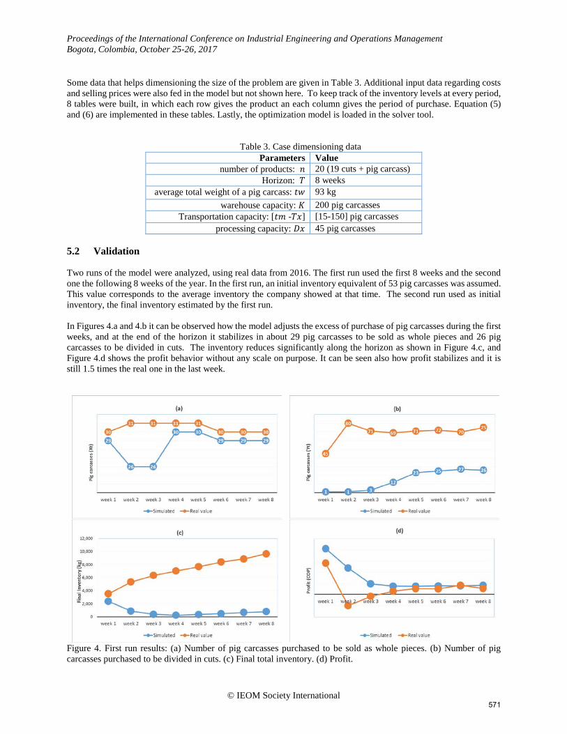
5.2 Validation Two runs of the model were analyzed, using real data from 2016. The first run used the first 8 weeks and the second one the following 8 weeks of the year. In the first run, an initial inventory equivalent of 53 pig carcasses was assumed. This value corresponds to the average inventory the company showed at that time. The second run used as initial inventory, the final inventory estimated by the first run. In Figures 4.a and 4.b it can be observed how the model adjusts the excess of purchase of pig carcasses during the first weeks, and at the end of the horizon it stabilizes in about 29 pig carcasses to be sold as whole pieces and 26 pig carcasses to be divided in cuts. The inventory reduces significantly along the horizon as shown in Figure 4.c, and Figure 4.d shows the profit behavior without any scale on purpose. It can be seen also how profit stabilizes and it is still 1.5 times the real one in the last week.

Figure 4. First run results: (a) Number of pig carcasses purchased to be sold as whole pieces. (b) Number of pig carcasses purchased to be divided in cuts. (c) Final total inventory. (d) Profit.



Figure 5. Second run results: (a) Number of pig carcasses purchased to be sold as whole pieces. (b) Number of pig carcasses purchased to be divided in cuts. (c) Final total inventory. (d) Profit. Figure 5 shows the results of the second run. In this run real data of the 8 weeks following the first run is compared. The model uses as initial inventory the final inventory simulated in the first run. Figure 5.a shows similar decisions on the number of pig carcasses to be sold as whole pieces while Figure 5.b shows a more stable difference in the number of pig carcasses to be divided in cuts, with an average difference of 18. This impacts directly on the average inventory, as shown in Figure 5.c. Finally, Figure 5.d shows a greater and more stable profit. Finally, Table 4 shows a summary of both runs. It shows reductions of more than 85% in the inventory in both cases, due to a reduction of about 30% of the number of pig carcasses to be purchased every week. Profit also increases. The first run shows157% increase and an adjustment can be observed in the behavior of the system. Run 2 starts with inventory that already reflects these changes, and shows a profit increase of almost 50%. However, as a consequence of smaller purchases, the shortages of the top 4 cuts increase up to 119.1%. It is worth noting that even in the real scenario, where purchases are 30% more, shortages are still present.

Table 4. Summary of results

Run 1 Run 2 Real Model Change Real Model Change

Total pig carcasses purchased 553 346 -37.4% 621 455 -26.7% Average inventory 7,092 767 -89.2% 13,353 1,764 -86.8% Total profit (thousand $COP) 21,844 56,202 157.3% 23,081 34,500 49.5% Shortages of 4 top cuts (kg) 8,277 14,872 79.7% 6,204 13,590 119.1%

6 Conclusions A forecasting – optimization methodology is proposed to improve inventory management in a small and young beef and pork retailer company in the city of Cali. The model considers fixed lifetime of the perishable products. To estimate sales, a forecasting model is selected for each product and these estimations are used as an input to the optimization model. The later maximizes profit, subject to capacity constraints. It tracks the age of the cuts in



inventory, which follows a FIFO policy, with nonlinear constraints. This is a very relevant aspect when it comes to perishable products. Inventory, transportation, processing and pig carcasses costs are considered in the model. Finally, an easy, user-friendly and accessible implementation on Excel was developed to select order size in a periodic revision system. The model was implemented and tested for an 8 week horizon, under two real scenarios. It showed potential improvements of more than 85% inventory reduction, a purchase reduction of about 30% of pig carcasses, and profit increase of 157% in the first run, and 49.5% in the second run. Future extensions of this model are to remove the assumption of having all initial inventory of one week old, and to adapt the model to beef, and to take care of shortages, which increases due to the purchase reductions.

References

Bakker, M., Riezebos, J., & Teunter, R. (2012). Review of inventory systems with deterioration since 2001. European Journal of Operational Research, 221(2), 275-284.

Deb, C., Zhang, F., Yanga, J., Leea, S. E., & Shaha, K. W. (2017). A review on time series forecasting techniques for building energy consumption. Renewable and Sustainable Energy Reviews, 74, 902-924.

Janssen, L., Claus, T., & Sauer, J. (2016). Literature review of deteriorating inventory models by key topics from 2012 to 2015. International Journal of Production Economics, 182, 86-112.

Lefcovich, M. (2004). Las pequeñas empresas y las causas de sus fracasos. Retrieved May 2017, from degerencia.com: (http://www.degerencia.com/articulo/las_pequenas_empresas_y_las_causas_de_sus_fracaso

Li, R., Lan, H., & Mawhinney, J. R. (2010). A Review on Deteriorating Inventory Study. Journal Service Science & Management, 3 , 117-129.

Mou, S., Robb, D. J., & DeHoratius, N. (2017). Retail Store Operations: Literature Review and Research Directions. European Journal of Operational Research, Accepted paper.

Myers, B. R. (2009). Analysis of an inventory system with product perishability and substitution: A simulation-optimization approach. Ph.D. thesis, Drexel University.

Pérez, F. A., & Torres, F. (2014). Inventory models with deteriorating item: a literature review. Ingeniería, 19(2), 9-40.

Raafat, F. (1991). Survey of Literature on Continuously Deteriorating Inventory Models. Journal of the Operational Research Society, 42(1), 27-37.

Vélez, M., & Castro, C. (2002). Modelo de Revisión Periódica para el Control del Inventario en Artículos con Demanda Estacional una Aproximación desde la Simulación. Dyna, 69(137), 23-34.

Vidal H., C. J. (2010). Fundamentos de control y gestión de inventarios. Cali: Programa Editorial Universidad del Valle.

Biography

Ivan Daniel Mesias is industrial engineer from Pontificia Universidad Javeriana – Cali (Jul, 2017). He works as operations analyst in Coomeva.

Fernando Alberto Osorio is industrial engineer from Pontificia Universidad Javeriana – Cali (Sep, 2017). He works as purchasing analyst in RTA furniture factory.

Jenny Díaz Ramírez is professor at the University of Monterrey. She has worked previously as a professor at Tecnologico de Monterrey, Mexico and Pontificia Universidad Javeriana Cali, Colombia. She got a MSc in operations research from Georgia Tech and the PhD in Industrial Engineering from Tecnologico de Monterrey, Campus Toluca in 2007. Her research areas are applied optimization and statistics in topics such as health systems, air quality and logistics.


Inventory Supply Model for Perishable Products - The ...ieomsociety.org/bogota2017/papers/95.pdf ·...

Documents

Transcript of Inventory Supply Model for Perishable Products - The ...ieomsociety.org/bogota2017/papers/95.pdf ·...